
Energy Markets Quantitative Analysis

Lecture 2: Forecasting Electricity Prices

Lecture 2

Forecasting Electricity Prices

Prof. dr. Daniel Traian PELE

Bucharest University of Economic Studies, Department of Statistics and Econometrics
Romanian Academy, Institute for Economic Forecasting

Every day before noon, a supplier, a producer or a battery operator in Romania has to decide how much electricity to buy or sell for each hour of the next day. The decision is taken on the day-ahead market, Piața pentru Ziua Următoare (PZU), run by the Romanian electricity and gas market operator (OPCOM), and the price at which it is settled is known only after the auction. This lecture asks a practical question: how well can tomorrow's hourly prices be forecast with the information available at 12:00 Central European Time (CET) on the day before delivery, and how do we know that one forecast is really better than another?

The answer is built step by step on real data: hourly Romanian day-ahead prices together with load, wind, solar, hydro, nuclear and cross-border flows from 1 Jan 2022 to 31 Oct 2026, with the last 365 days kept as a test year. We start from a naive rule that any trader could apply, measure errors in EUR/MWh, and test differences between models statistically. We then build expert regression models, shrink them with a penalty that selects the regressors automatically, average forecasts across calibration windows and across models, preview machine learning and turn point forecasts into intervals. The lecture ends with the cointegration tests announced in Lecture 1 and with four case studies that translate forecast accuracy into money.

The discipline matters as much as the models. A backtest that uses information which was not yet available at the auction looks excellent and cannot be run on a real trading desk. Every number in this lecture comes from forecasts that obey the 12:00 rule, and the lecture shows how to check it.

Learning outcomes

  • Set up a day-ahead forecast that uses only what is known at 12:00 CET on the day before delivery.
  • Measure accuracy with the mean absolute error (MAE), the root mean squared error (RMSE) and the relative MAE (rMAE), and test differences between models with the Diebold–Mariano (DM) test.
  • Build expert autoregressive models with exogenous variables (ARX), shrink them with the least absolute shrinkage and selection operator (LASSO) and obtain the LASSO-estimated autoregression (LEAR).
  • Combine forecasts, preview machine learning (ML) and turn point forecasts into quantiles with quantile regression averaging (QRA).
  • Test cointegration of Romania with Hungary, and of power with gas and hydro, as announced in Lecture 1.

Lecture plan

  1. The forecasting problem and its benchmarksBefore any model is estimated, the forecasting problem has to be defined precisely: which prices are forecast, at what moment, with which information, and against which benchmark the result is judged.
  2. Expert models: ARX and LEARExpert models are linear regressions whose inputs are the variables a trader looks at first: recent prices, the calendar and the fundamentals of supply and demand.
  3. Windows, combinations and machine learningNo single model or calibration window is best at all times.
  4. Probabilistic forecasts and cointegrationA point forecast is not enough for risk management, and prices of neighbouring markets or of fuels are linked in the long run.
  5. Case studies on recent Romanian dataFour case studies apply the models of the lecture to recent Romanian data and translate accuracy into the questions a manager asks: how stable the accuracy is over the year, what happens in a stress week, how to forecast the new quarter-hour prices and what a better forecast is worth in euros.
  6. Wrap-upThe wrap-up tests the main ideas with five short questions, summarises the lecture and lists the research of our group and further reading.
  7. AppendixThe appendix gives the technical details behind the main slides: the full specification of LEAR, the accuracy by quarter, the probabilistic scores with the Kupiec test, and all unit-root and cointegration tests.

The forecasting problem and its benchmarks

Before any model is estimated, the forecasting problem has to be defined precisely: which prices are forecast, at what moment, with which information, and against which benchmark the result is judged. This section fixes the timing of the day-ahead auction, the split of the data into calibration, burn-in and test periods, the naive benchmark, the error measures and the statistical test used to compare models.

Forecast target and data sources

Slide 5 in the PDF

The target of the lecture is the hourly day-ahead price of the Romanian bidding zone (RO) on the PZU, published by OPCOM and downloaded through energy-charts.info, the data portal of the Fraunhofer Institute for Solar Energy Systems (ISE), which takes it from the European Network of Transmission System Operators for Electricity (ENTSO-E). The explanatory series are the hourly and daily load, wind and solar, hydro and nuclear generation and cross-border flows from ENTSO-E (Transelectrica data for Romania); the price of carbon, proxied by the SparkChange physical European Union (EU) emission allowance (EUA) exchange-traded commodity (ETC) from Yahoo Finance; the prices of the neighbouring zones, Hungary (HU) from the Hungarian Power Exchange (HUPX) and the Germany–Luxembourg bidding zone (DE-LU) from the EPEX SPOT power exchange (EPEX); and the monthly gas price at the Dutch Title Transfer Facility (TTF) from the World Bank Pink Sheet.

The data end on 31 Oct 2026 and were downloaded on 4 Nov 2026. The panel runs from 1 Jan 2022 to 31 Oct 2026 and contains 1,765 complete days. The test year is the last 365 days, 1 Nov 2025 to 31 Oct 2026; the 182 days before it form a burn-in period used only to calibrate the prediction intervals. Daylight saving time (DST) is handled as in Assignment 1: every day has 24 columns, the missing spring hour is the mean of its neighbours and the doubled autumn hour is averaged. The 2 DST days of the test year are kept in the evaluation.

Day-ahead market: the auction on d-1 sets the prices of day d

Slide 7 in the PDF

The PZU is one daily auction of the Single Day-Ahead Coupling (SDAC), the mechanism that couples the European day-ahead markets; in Romania it is run by OPCOM. On the trading day \(d-1\), buyers and sellers submit orders, pairs of quantity and price, for every delivery period of the next day \(d\). At 12:00 CET the order books close (gate closure). A common algorithm, the Pan-European Hybrid Electricity Market Integration Algorithm (EUPHEMIA), then matches supply and demand across the coupled zones, and the results are normally published around 13:00 CET (NEMO Committee, 2025, 2026).

Since 1 October 2025 the auction sets 96 quarter-hour prices per day instead of 24 hourly prices. The data used in this lecture define the hourly price as the mean of the four quarter-hours of each hour, and this definition is applied over the whole test year, so the hourly series remains comparable before and after the change. Case study (c) at the end of the lecture returns to the quarter-hours.

The timeline matters because it fixes what a forecaster can know. The forecast for day \(d\) must be ready before the gate closes at noon on \(d-1\), while day \(d\) itself starts only twelve hours later and ends 36 hours after the auction.

Notation and the information rule for all forecasts

Slide 8 in the PDF

The lecture uses a fixed notation. The delivery day is \(d\); \(d-1\) is the day before, when the auction runs; \(d-2\) is two days before. The hour of delivery is \(h=0,\dots,23\) in CET, \(P_{d,h}\) is the day-ahead price of hour \(h\) on day \(d\) in EUR/MWh (euro per megawatt-hour) and \(\hat P_{d,h}\) is its forecast.

The rule that every forecast in this lecture obeys is simple: the forecast for day \(d\) is made before 12:00 CET on day \(d-1\), so it may use only what is known at that moment. All 24 prices of day \(d-1\) are allowed, because they were fixed by the auction on day \(d-2\). The load, wind and solar forecasts for day \(d\) published by the transmission system operator (TSO) before noon would also be allowed. What is not allowed is any realised value of day \(d\), or any value of day \(d-1\) that has not yet been metered.

The object of the exercise is therefore the 24 hourly prices of the Romanian PZU for each day of the test year. The error \(P_{d,h}-\hat P_{d,h}\) becomes known only after day \(d\) has been delivered, so the evaluation is always out of sample (Lago et al., 2021).

In practice: the same rule binds a real trading desk: a model that breaks it cannot be run at 12:00.

Information set at 12:00 CET on day \(d-1\)

Slide 9 in the PDF

The slide draws the information set on a time line. The prices of day \(d-1\) were published around 13:00 on day \(d-2\). The last complete metered day is \(d-2\), which ends at midnight before the trading day. At 12:00 on \(d-1\) the forecast and the bids for day \(d\) are sent, and the 24 hourly (96 quarter-hour) prices of day \(d\) are what has to be forecast.

The models of this lecture therefore use prices up to \(d-1\); realised load, wind, solar, hydro, nuclear generation and cross-border flows up to \(d-2\); and the carbon price at the close of \(d-2\). What is not in our free data are the day-ahead load and renewable forecasts of the TSO, which a real desk would use. This is a handicap for our models, not an error: they are legal, but we do not have them. Later slides show that this is exactly where most of the possible improvement lies.

In practice: a backtest that uses the realised load of \(d-1\) looks excellent and cannot be run at 12:00.

Chronological split into calibration, burn-in and test periods

Slide 10 in the PDF

A forecasting model for prices must be evaluated in the same order in which it would be used. Each model is re-estimated every day on a window that ends at \(d-1\), then produces the 24 forecasts for day \(d\); the window then moves forward by one day. There is no random K-fold cross-validation and no random validation split, because shuffling the days would let the model learn from the future and would make the backtest look better than reality (Weron, 2014; Lago, Marcjasz, De Schutter & Weron, 2021).

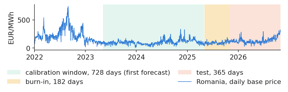
The chart shows how the sample is used. The first forecast is made with a calibration window of 728 days; the following 182 days form the burn-in, whose forecasts serve only to calibrate the prediction intervals; and the last 365 days form the test year on which every error in this lecture is measured. The test year is touched once, at the end.

In practice: ask any vendor for the rolling backtest, not an in-sample fit.
Chart: Chronological split into calibration, burn-in and test periods

Daily base price of Romania from 1 Jan 2022 to 31 Oct 2026, in EUR/MWh, with the first 728-day calibration window, the 182-day burn-in and the 365-day test period shaded.

Source: energy-charts.info (Fraunhofer ISE); OPCOM day-ahead prices for Romania, via ENTSO-E. Data: daily base price, 2022-01-01 to 2026-10-31, CET delivery days.

Forecast error grows with the age of the information, except at the weekly lag

Slide 11 in the PDF

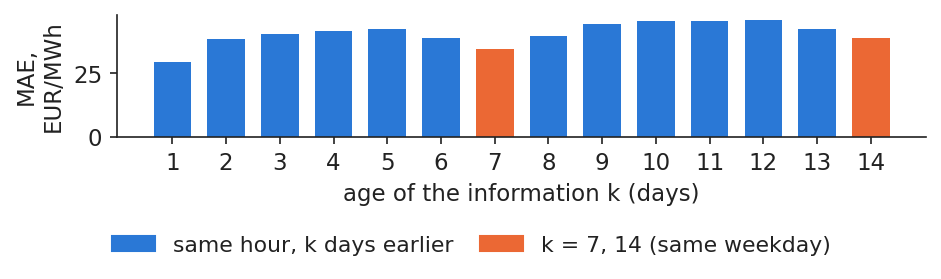
The simplest possible forecast copies the price of the same hour \(k\) days earlier, \(\hat P_{d,h}=P_{d-k,h}\). The chart shows its MAE on the test year as a function of the age \(k\) of the information. With yesterday's price, \(k=1\), the MAE is 29.37 EUR/MWh. With the price of two days earlier it rises to 38.52, because the information is older. At \(k=7\), however, the error falls back to 34.41, since the same weekday a week earlier shares the weekly pattern of consumption.

Two conclusions follow. The freshest information is the most valuable, so any honest model will lean heavily on the prices of \(d-1\). And the weekly cycle is strong enough that a week-old price can beat a more recent one on some days, which motivates the naive benchmark defined two slides later.

In practice: the day-ahead horizon is 12 to 36 hours, and the freshest price you hold at 12:00 is that of \(d-1\).
Chart: Forecast error grows with the age of the information, except at the weekly lag

MAE of the forecast that copies the price of the same hour \(k\) days earlier, for \(k\) from one to 14 days, test year; bars for \(k\) = 7 and 14 (same weekday) are highlighted.

Source: energy-charts.info (Fraunhofer ISE); OPCOM day-ahead prices for Romania, via ENTSO-E. Data: test year 2025-11-01 to 2026-10-31, hourly.

Point, probabilistic and path forecasts answer different questions

Slide 12 in the PDF

A forecast can take three forms. A point forecast gives one number per hour; a probabilistic forecast gives the distribution of the price, for example as a set of quantiles; a path forecast gives joint scenarios for all 24 hours:

\[\underbrace{\hat P_{d,h}}_{\text{point}}\qquad\underbrace{\hat q^{\tau}_{d,h}:\ \Pr(P_{d,h}\le \hat q^{\tau}_{d,h})=\tau}_{\text{quantile}}\qquad \underbrace{\{\hat P^{(s)}_{d,0},\dots,\hat P^{(s)}_{d,23}\}_{s=1}^{S}}_{\text{paths}}\]
(2.1)

where \(d\) is the delivery day, \(h\) the hour in CET, \(\hat q^{\tau}_{d,h}\) the quantile of level \(\tau\in(0,1)\), \(s\) indexes the scenario and \(S\) is the number of scenarios.

The difference matters because the errors of different hours are not independent. On the Romanian test year the forecast errors at 12 h and 13 h correlate at 0.96, while those at 3 h and 19 h correlate at only 0.13. A set of 24 separate quantiles cannot describe such dependence; paths can. Each user needs a different object (Nowotarski & Weron, 2018): a supplier buying a block of hours needs the point forecast, a risk manager needs quantiles (Lecture 4), and a battery needs paths, because it buys in one hour and sells in another, so what matters is the joint behaviour of the two prices.

In practice: decide which of the three your decision needs before you buy a forecast.

The naive benchmark: yesterday, or last week for Monday and the weekend

Slide 13 in the PDF

Every model must beat the rule a trader would use without any model. The standard naive benchmark of the literature (Nogales et al., 2002; Weron, 2014) takes yesterday's price on working days in the middle of the week and last week's price on days whose pattern differs from the day before:

\[\hat P^{\text{naive}}_{d,h}=\begin{cases}P_{d-7,h}, & \text{Mon, Sat, Sun}\\ P_{d-1,h}, & \text{Tue–Fri}\end{cases}\]
(2.2)
\[\hat P^{(7)}_{d,h}=P_{d-7,h}\]
(2.3)

where \(P_{d,h}\) is the price of day \(d\) and hour \(h\) in EUR/MWh and \(\hat P^{(7)}\) in (2.3) is the seasonal naive forecast, the same hour of the previous week.

The switch is justified by the data. On Mondays, Saturdays and Sundays, the price of \(d-7\) gives an MAE of 29.87 EUR/MWh against 33.48 for the price of \(d-1\), because Monday follows a weekend and the weekend follows a working day. From Tuesday to Friday the order reverses: 26.27 for \(d-1\) against 37.83 for \(d-7\). Over the whole test year the naive rule has an MAE of 27.82 EUR/MWh and the seasonal naive one 34.41. With a mean price of 134.46 EUR/MWh, the naive error is about one fifth of the price.

In practice: ask any forecast vendor for the rMAE against this naive rule on your hours.

Four error measures and the relative MAE

Slide 14 in the PDF

Forecast errors can be summarised in several ways, and each answers a slightly different question (Hyndman & Koehler, 2006). With \(e_{d,h}=P_{d,h}-\hat P_{d,h}\):

\[\text{MAE}=\tfrac1N\textstyle\sum|e_{d,h}|,\qquad \text{RMSE}=\sqrt{\tfrac1N\textstyle\sum e_{d,h}^2}\]
(2.4)
\[\text{sMAPE}=\tfrac1N\textstyle\sum\frac{2|e_{d,h}|}{|P_{d,h}|+|\hat P_{d,h}|},\qquad \text{rMAE}=\frac{\text{MAE}_{\text{model}}}{\text{MAE}_{\text{naive}}}\]
(2.5)

where \(N\) is the number of (day, hour) pairs and the sums run over all of them. The symmetric mean absolute percentage error (sMAPE) is bounded by 200%. The rMAE divides the MAE of a model by the MAE of the naive benchmark (2.2) on the same hours, so a value below 1 means the model is better than naive.

The MAE is in EUR/MWh and is easy to explain; the RMSE squares the errors and therefore punishes spikes more. The MAE is minimised by the median forecast, the RMSE by the mean. On the test year the naive rule has MAE 27.82, RMSE 44.54 and sMAPE 34.5%. LEAR averaged across calibration windows (AW-LEAR), introduced later, reaches MAE 22.53, RMSE 36.35 and rMAE 0.810. The best model of the lecture, an ensemble of 4, has rMAE 0.795, that is 20.5% less error than naive.

In practice: report MAE in EUR/MWh to the desk and rMAE to management, on the same hours.

Limitations of percentage errors near zero and negative prices

Slide 15 in the PDF

The mean absolute percentage error (MAPE) is popular in business reports, but it does not work for electricity prices:

\[\text{MAPE}=\tfrac1N\textstyle\sum|e_{d,h}|/|P_{d,h}|\]
(2.6)

with the same \(e_{d,h}\), \(P_{d,h}\) and \(N\) as in (2.4). The problem is the denominator. When the price is close to zero, as happens in sunny hours with high solar output, even a small error in EUR/MWh becomes an enormous percentage, and when the price is negative the measure loses its meaning altogether.

On the Romanian test year the MAPE of AW-LEAR is 5,777.7%. Without the 387 hours in which the absolute price is below 5 EUR/MWh it falls to 32.4%. These few hours produce 99.5% of the MAPE. The chart plots, for every hour of the test year, the absolute percentage error against the actual price: the errors explode in the narrow band around zero, while elsewhere they stay moderate. The same forecast can therefore look either reasonable or catastrophic depending only on the measure chosen (Hyndman & Koehler, 2006; Weron, 2014).

In practice: never accept a MAPE for power prices; ask for MAE and rMAE.

Interactive chartInteractive page →

    Code of this chart: EMQA_L2_mape_fail · open in Colab

    Absolute percentage error of the AW-LEAR forecast against the actual price for each of the 8,760 hours of the test year, with the band \(|P|<5\) EUR/MWh shaded and the 100% error line marked.

    Source: energy-charts.info (Fraunhofer ISE); OPCOM prices; ENTSO-E load, wind and solar (Transelectrica data for Romania). Data: test year 2025-11-01 to 2026-10-31, 8760 hours.

    Question for the room The test year has 8,760 hours. The MAPE of AW-LEAR is above 5,700%, its MAE 22.53 EUR/MWh. Is the model really that bad?
    Answer

    No. The percentage error divides by the actual price, and 387 hours have |price| below 5 EUR/MWh (60 are exactly zero, 195 are negative). These hours produce 99.5% of the MAPE; excluding them, the MAPE of AW-LEAR falls to 32.4%. Move the slider: the MAE and the sMAPE hardly change, the MAPE collapses. With prices near zero, MAE, RMSE and the relative MAE (rMAE, MAE divided by the MAE of the naive forecast) are the measures to report.

    The Diebold–Mariano test of equal predictive accuracy

    Slide 16 in the PDF

    A lower MAE on one test year may be due to luck. The Diebold–Mariano test (Diebold & Mariano, 1995) asks whether the mean difference in errors between two models is large relative to its own noise. Following Ziel & Weron (2018), the 24 hourly errors are first averaged within each day, which removes the strong correlation between the hours of the same day (the multivariate version of the test):

    \[\Delta_d=\underbrace{\tfrac1{24}\textstyle\sum_h|e^{A}_{d,h}|}_{\text{model A}}-\underbrace{\tfrac1{24}\textstyle\sum_h|e^{B}_{d,h}|}_{\text{model B}},\qquad \text{DM}=\frac{\bar\Delta}{\sqrt{\hat\sigma^2_{\Delta}/n}}\]
    (2.7)

    where \(e^{A}_{d,h}\) and \(e^{B}_{d,h}\) are the errors of models A and B, \(\Delta_d\) is the difference in their daily mean absolute errors, \(\bar\Delta\) its mean over the \(n\) test days, \(\hat\sigma^2_{\Delta}\) its Newey–West variance with 7 lags, and the one-sided p-value is \(p=1-\Phi(\text{DM})\), with \(\Phi\) the standard normal distribution function. A small \(p\) means that B is more accurate than A.

    On the 365 test days, naive against AW-LEAR gives DM = 7.32 with \(p<0.001\): LEAR is clearly better. ARX averaged across windows (AW-ARX) against AW-LEAR gives DM = −0.83 and \(p\) = 0.797, so there is no significant difference. AW-LEAR against the ensemble of 4 gives DM = 2.21 and \(p\) = 0.014: the ensemble is significantly better.

    In practice: switch models only when the gain is significant on your hours.

    Pairwise DM tests on the Romanian test year

    Slide 17 in the PDF

    Running the DM test of (2.7) for every pair of models gives a matrix of p-values. Rows carry the model names and numbers, columns the same numbers. Each cell answers the question "is the column model more accurate than the row model?", and green cells mark a significant win of the column model. The diagonal is empty.

    On the Romanian test year, 8 of the 9 other models beat the naive benchmark at the 5% level; the exception is the seasonal naive forecast, which is worse. Columns with many green cells belong to models that beat most of the others. The matrix is a compact way to read a model comparison without being misled by small differences in MAE that are not statistically meaningful (Ziel & Weron, 2018; Lago et al., 2021).

    In practice: read a column top to bottom: many green cells mean a model worth paying for.

    Interactive chartInteractive page →

      Code of this chart: EMQA_L2_dm_matrix · open in Colab

      One-sided p-values of the DM test for each pair of models on the 365 test days, capped at 0.10; green cells mark a significant win of the column model over the row model.

      Source: energy-charts.info (Fraunhofer ISE); OPCOM prices; ENTSO-E generation and flows (Transelectrica data for Romania); Yahoo Finance (SparkChange EUA ETC). Data: test year 2025-11-01 to 2026-10-31, 365 days; one-sided p-values.

      Question for the room AW-LEAR has an MAE of 22.53 EUR/MWh, the naive forecast 27.82. Is the difference significant, and is AW-LEAR significantly better than AW-ARX (22.30)?
      Answer

      The first yes, the second no. The DM test works on the daily loss differential d_t (mean over the 24 hours of |e_A| − |e_B|) with a Newey–West variance (7 lags): naive vs AW-LEAR gives DM = 7.32, one-sided p < 0.001; AW-ARX vs AW-LEAR gives DM = −0.83, p = 0.80, so AW-LEAR is not more accurate than AW-ARX. Change the loss to squared errors or the number of lags: the sign of the conclusion for naive vs AW-LEAR does not change; for close models it can.

      Section summary

      A forecast for the PZU must use only what is known at 12:00 CET on \(d-1\), be evaluated on a rolling test year, and be compared with the naive benchmark in EUR/MWh and in rMAE, with the DM test to separate real gains from luck.

      Expert models: ARX and LEAR

      Expert models are linear regressions whose inputs are the variables a trader looks at first: recent prices, the calendar and the fundamentals of supply and demand. This section builds the ARX model, shows how its coefficients vary by hour, transforms prices to tame spikes and then lets the LASSO choose the regressors automatically in the LEAR model.

      The expert ARX model: recent prices, calendar and fundamentals

      Slide 19 in the PDF

      The ARX model is one linear regression per hour with the inputs a trader looks at first (Ziel & Weron, 2018; Weron, 2014):

      \[Y_{d,h}=\beta_0+\underbrace{\beta_1Y_{d-1,h}+\beta_2Y_{d-2,h}+\beta_3Y_{d-7,h}}_{\text{autoregression}}+\underbrace{\beta_4Y_{d-1,23}+\beta_5Y^{\min}_{d-1}+\beta_6Y^{\max}_{d-1}}_{\text{yesterday's shape}}+\underbrace{\beta_7\tilde L_{d,h}+\beta_8\tilde R_{d,h}}_{\text{fundamentals of } d-2}+\underbrace{\textstyle\sum_{j}\delta_jD^{j}_d}_{\text{Mon, Sat, Sun}}+\varepsilon_{d,h}\]
      (2.8)

      where \(Y_{d,h}\) is the asinh-transformed price of hour \(h\) on day \(d\) (the transformation is defined below); \(Y_{d-1,h}\), \(Y_{d-2,h}\) and \(Y_{d-7,h}\) are the prices of the same hour one, two and seven days earlier; \(Y_{d-1,23}\) is the last hour of yesterday and \(Y^{\min}_{d-1}\), \(Y^{\max}_{d-1}\) yesterday's minimum and maximum; \(\tilde L_{d,h}=L_{d-2,h}\) is the load and \(\tilde R_{d,h}\) the wind and solar generation of the same hour on \(d-2\), both z-scored; \(D^{j}_d\) are dummies for Monday, Saturday and Sunday with coefficients \(\delta_j\); \(\beta_0,\dots,\beta_8\) are coefficients and \(\varepsilon_{d,h}\) is the error.

      The model is estimated by ordinary least squares (OLS), separately for each of the 24 hours, with 12 regressors per hour, as in Assignment 1. On our data the ARX(728) version, estimated on a 728-day window and re-estimated every day, has MAE 22.72 EUR/MWh and rMAE 0.817, already almost a fifth better than naive.

      In practice: this is the model to beat before anyone sells you a neural network.

      The ARX coefficients change with the hour of the day

      Slide 20 in the PDF

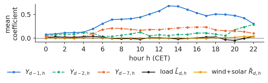
      Because a separate regression is estimated for each hour, the coefficients of (2.8) can differ across the day. The chart shows the mean of each coefficient over the 365 daily fits of the test year, hour by hour. The weight of yesterday's same hour, \(Y_{d-1,h}\), is largest at hour 13 (0.68) and smallest at hour 0 (0.08). Night hours lean instead on the last hour of \(d-1\), whose coefficient reaches up to 0.73: just after midnight the closest price in time is the one of the previous evening, not the one of the same hour 24 hours earlier.

      The coefficients of load and of wind and solar stay close to zero in every hour. Observed on day \(d-2\), these fundamentals add little to what yesterday's price already contains. The hourly pattern of the coefficients is the reason why one model per hour is used rather than a single equation.

      In practice: one model per hour lets the evening peak learn from different drivers than the night.
      Chart: The ARX coefficients change with the hour of the day

      Mean ARX(728) coefficients by hour (CET) over the 365 daily fits of the test year, for the prices of \(d-1\), \(d-2\) and \(d-7\), the load and the wind + solar generation.

      Source: energy-charts.info (Fraunhofer ISE); OPCOM prices; ENTSO-E load, wind and solar (Transelectrica data for Romania). Data: ARX(728), mean over the 365 daily fits of the test year.

      Small contribution of fundamentals lagged by two days

      Slide 21 in the PDF

      The table compares three versions of ARX(728) on the test year. With prices and calendar only, the MAE is 22.63 EUR/MWh. Adding the load and wind + solar generation of \(d-2\) gives 22.72, and adding also hydro, nuclear, net imports and the EUA of \(d-2\) leaves the MAE at 22.72. The fundamentals do not improve the forecast.

      ARX(728), test yearMAERMSErMAE
      prices and calendar only22.6336.490.813
      + load, wind + solar of d-222.7236.620.817
      + hydro, nuclear, net imports, EUA of d-222.7236.500.817

      Fundamentals missing on a given day are carried forward from the past only (this was needed for nuclear on 29 days). The EUA is the closing price of the SparkChange ETC on \(d-2\), a proxy of the allowance price.

      The reason is timing. What happened on \(d-2\) is already reflected in the price of \(d-1\), which the model sees anyway; an outage of the Cernavodă nuclear power plant, for instance, reaches the model two days late. What would help are the published day-ahead forecasts of load, wind and solar for day \(d\) itself (ENTSO-E, Transelectrica). They are legal at 12:00 on \(d-1\), but they are not part of our free data (Lago et al., 2021).

      In practice: buy the TSO's day-ahead load and renewable forecasts before buying a more complex model.

      Separate models for each hour are more accurate than a single model

      Slide 22 in the PDF

      An alternative to 24 hourly regressions is a single pooled regression for all hours, with hour-specific intercepts but common slopes. The pooled model is simpler and uses 24 times more observations per coefficient, but it forces every hour to react in the same way to yesterday's price and to the fundamentals.

      On the test year the per-hour ARX(728) has MAE 22.72 EUR/MWh, while the pooled version reaches 24.54. The chart shows the MAE by hour for both and for the naive benchmark: the pooled model is worse in 21 of the 24 hours. The gain from separate hourly models is consistent with the different coefficient profiles seen on the previous slide (Ziel & Weron, 2018).

      In practice: since 1 Oct 2025 the same choice arises for the 96 quarter-hours.

      Interactive chartInteractive page →

      Models

        Code of this chart: EMQA_L2_per_hour_single · open in Colab

        MAE by hour (CET) on the test year for the naive benchmark, ARX(728) with one model for all hours and ARX(728) with one model per hour.

        Source: energy-charts.info (Fraunhofer ISE); OPCOM prices; ENTSO-E load, wind and solar (Transelectrica data for Romania). Data: test year 2025-11-01 to 2026-10-31.

        Question for the room ARX(728) estimates one regression per hour (24 models); the single-regression version uses common slopes and only hour-specific intercepts. In how many hours is the single regression worse?
        Answer

        In 21 of the 24 hours. Its MAE over the year is 24.54 EUR/MWh, against 22.72 for ARX(728) with one regression per hour: each hour has its own dynamics (night hours follow the previous day closely, the solar hours depend more on renewables). The errors of all models peak in the evening: AW-LEAR has its worst hour at 19:00 (34.52 EUR/MWh) and its best at 01:00 (9.47).

        The asinh transformation for price spikes and negative prices

        Slide 23 in the PDF

        Electricity prices have spikes and can be negative, so a regression on raw prices is dominated by a few extreme hours. A variance-stabilising transformation (VST) compresses the extremes before estimation (Uniejewski, Weron & Ziel, 2018). The lecture uses the inverse hyperbolic sine:

        \[Y=\asinh\!\left(\frac{P-m}{s}\right)\]
        (2.9)

        where \(P\) is the price, \(m\) its median and \(s\) = 1.4826 × the median absolute deviation (MAD), both computed from the calibration window only, so that no future information enters the transformation. Forecasts are made on the \(Y\) scale and transformed back with the hyperbolic sine.

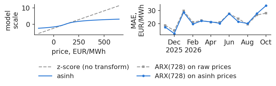
        The left panel of the chart shows the transformation: close to the median it is almost linear, far from it it grows only logarithmically, and unlike the logarithm it is defined for negative prices. The right panel compares the monthly MAE of ARX(728) with and without the transformation. Over the test year the MAE is 22.86 on raw prices and 22.72 with asinh. The RMSE goes the other way (35.85 raw against 36.62 with asinh), because the transformation gives less weight to spikes when fitting.

        In practice: asinh works below zero, where the logarithm cannot be used.
        Chart: The asinh transformation for price spikes and negative prices

        Left: the asinh transformation and a plain z-score against the price, with the median and scale of the last window; right: monthly MAE of ARX(728) on raw and on asinh-transformed prices over the test year.

        Source: energy-charts.info (Fraunhofer ISE); OPCOM prices; ENTSO-E load, wind and solar (Transelectrica data for Romania). Data: left, median and scale of the last window; right, test year 2025-11-01 to 2026-10-31.

        LEAR: LASSO selection among 247 candidate regressors

        Slide 24 in the PDF

        Instead of choosing the regressors by expert judgement, the LEAR model gives the regression many candidates and lets a penalty select them (Tibshirani, 1996; Uniejewski, Nowotarski & Weron, 2016; Lago et al., 2021). For each hour \(h\):

        \[\hat{\boldsymbol\beta}_h=\arg\min_{\boldsymbol\beta}\Big\{\underbrace{\textstyle\sum_{d\in\text{cal}}(Y_{d,h}-\mathbf x_d^{\top}\boldsymbol\beta)^2}_{\text{fit}}+\underbrace{\lambda_h\textstyle\sum_j|\beta_j|}_{\text{penalty}}\Big\}\]
        (2.10)

        where the sum runs over the days of the calibration window, \(Y_{d,h}\) is the transformed price, \(\mathbf x_d\) is the vector of 247 regressors (all 24 prices of \(d-1\), \(d-2\), \(d-3\) and \(d-7\), that is 96; the load and the wind + solar generation of \(d-2\), \(d-3\) and \(d-7\), that is 144; and 7 weekday dummies), \(\boldsymbol\beta\) the vector of coefficients \(\beta_j\), and \(\lambda_h\ge0\) the strength of the penalty, chosen every day by the Akaike information criterion (AIC) inside the window. The absolute-value penalty sets the useless coefficients exactly to zero, so the data choose the regressors.

        On our data LEAR(728) keeps on average 42 of the 247 regressors (17%), between 8 and 121 depending on the hour and the day. Its MAE is 22.62 EUR/MWh; averaging the forecasts estimated on windows of 364, 546 and 728 days (AW-LEAR) gives 22.53. The penalty must be chosen honestly: by an information criterion, or on a validation block that ends before the forecast day, and never on the test year.

        In practice: a LASSO model explains itself, since the kept regressors show what drives each hour.

        Regressors selected by LEAR: yesterday's same hour and the weekday, rarely the lagged fundamentals

        Slide 25 in the PDF

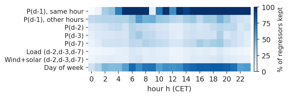
        Because the LASSO sets coefficients exactly to zero, one can count how often each group of regressors survives. The heat map shows, for each hour of the day and each group of candidate regressors, the share kept by LEAR(728) over the 365 daily fits of the test year.

        On average, yesterday's price of the same hour, \(P_{d-1,h}\), is kept in 79% of the fits and the weekday dummies in 64%. By contrast, only 9% of the load regressors and 11% of the wind + solar regressors are kept. The LASSO confirms the finding of the ARX experiment: fundamentals observed two days before delivery carry little information that is not already in the price of \(d-1\).

        In practice: real gains need forecasts of the fundamentals for day \(d\).
        Chart: Regressors selected by LEAR: yesterday's same hour and the weekday, rarely the lagged fundamentals

        Share of regressors kept by LEAR(728), in %, by group of regressors (rows) and hour of the day (columns), over the 365 daily fits of the test year.

        Source: energy-charts.info (Fraunhofer ISE); OPCOM prices; ENTSO-E load, wind and solar (Transelectrica data for Romania). Data: LEAR(728), 365 daily fits of the test year.

        Section summary

        The expert ARX model with one regression per hour already cuts the naive error by almost a fifth; the asinh transformation handles spikes and negative prices; and the LASSO selects a small set of regressors, mostly recent prices and the weekday, while fundamentals lagged by two days add almost nothing.

        Windows, combinations and machine learning

        No single model or calibration window is best at all times. This section averages forecasts across calibration windows and across models, presents the scoreboard of the Romanian test year and previews two machine-learning models, gradient boosting and a neural network, that are developed in Lecture 7.

        Averaging forecasts across calibration windows

        Slide 27 in the PDF

        The length of the calibration window is a hard choice. A short window adapts quickly when the market changes; a long window gives more stable estimates. Instead of guessing the best length, the model can be estimated on several windows and the forecasts averaged (Hubicka, Marcjasz & Weron, 2019; Marcjasz, Serafin & Weron, 2018):

        \[\hat P^{\text{AW}}_{d,h}=\frac1{|\mathcal T|}\sum_{T\in\mathcal T}\hat P^{(T)}_{d,h}\]
        (2.11)

        where \(\hat P^{(T)}_{d,h}\) is the forecast of the model estimated on a rolling window of the last \(T\) days, re-estimated daily, \(\mathcal T\) is the set of window lengths and \(|\mathcal T|\) their number. For ARX, \(\mathcal T=\{56,84,112,714,721,728\}\); for LEAR, \(\mathcal T=\{364,546,728\}\). This is averaging across calibration windows (AW).

        On our data the MAE of ARX is 24.44 EUR/MWh with a 56-day window, 23.41 with 112 days and 22.72 with 728 days. The average, AW-ARX, reaches 22.30, better than every single window. For LEAR the values are 22.96 for LEAR(364), 22.62 for LEAR(728) and 22.53 for AW-LEAR. Mixing short (56–112 days) and long (714–728 days) windows gives both adaptation and stability.

        In practice: when the market changes regime (2022, 2024), short windows react first; keep them in the average.

        Averaging across windows is more accurate than the best single window

        Slide 28 in the PDF

        The chart shows the MAE of each calibration window for ARX and LEAR, with the averaged forecast as the last bar of each panel and the naive benchmark of 27.82 EUR/MWh as a dotted line. For ARX, the averaged forecast AW-ARX has MAE 22.30 EUR/MWh, below the best single window, ARX(714), at 22.68.

        The result is useful precisely because the best window is not known in advance: on another year a short window might win. Averaging removes the need to choose and still delivers a result at least as good as the best choice made with hindsight (Hubicka, Marcjasz & Weron, 2019).

        In practice: you do not need to know the right window in advance: average a short and a long one.

        Interactive chartInteractive page →

        Windows in the average (days)

          Code of this chart: EMQA_L2_windows · open in Colab

          MAE on the test year for ARX (left) and LEAR (right) by calibration window \(T\) in days, with the window-averaged forecast (AW) and the naive benchmark as a dotted line.

          Source: energy-charts.info (Fraunhofer ISE); OPCOM prices; ENTSO-E load, wind and solar (Transelectrica data for Romania). Data: test year 2025-11-01 to 2026-10-31.

          Question for the room ARX with a 56-day window has an MAE of 24.44 EUR/MWh, with 728 days 22.72. Does the average of the forecasts across the six ARX windows beat the best single window?
          Answer

          Yes. AW-ARX, the average across the windows 56, 84, 112, 714, 721 and 728 days, has an MAE of 22.30 EUR/MWh, below every single window (best: 714 days, 22.68). Short windows adapt quickly to new price levels, long ones estimate the coefficients precisely; their errors are not perfectly correlated, so averaging reduces the error. Untick windows to see which combinations still help. For LEAR, the average of 364, 546 and 728 days (22.53) also beats each window (best: 728 days, 22.62).

          Combining different models: errors that do not coincide cancel out

          Slide 29 in the PDF

          If two models are wrong on different days, their simple average is wrong less often than either. With \(K\) models and equal weights (Bates & Granger, 1969; Nowotarski & Weron, 2015):

          \[\hat P^{\text{ens}}_{d,h}=\frac1K\sum_{k=1}^{K}\hat P^{(k)}_{d,h},\qquad \Var(\bar e)=\frac{\bar\sigma^2}{K}\big(1+(K-1)\bar\rho\big)\]
          (2.12)

          where \(\hat P^{(k)}_{d,h}\) is the forecast of model \(k\), \(K\) the number of models, \(\bar e\) the error of the average forecast, \(\bar\sigma^2\) the average error variance of the models and \(\bar\rho\) the average correlation of their errors. The lower \(\bar\rho\), the larger the gain; with perfectly correlated errors averaging brings nothing. Equal weights need no estimation, which makes them robust.

          On our data the ensemble of 4 averages AW-ARX, AW-LEAR, a gradient boosting machine (GBM) and a multilayer perceptron (MLP) with equal weights. It has MAE 22.13 EUR/MWh and rMAE 0.795, the best of all models. It is better than AW-LEAR in 8 of the 12 months and in 15 of the 24 hours, and the DM test against AW-LEAR gives \(p\) = 0.014. The two weaker members, GBM and MLP, still help, because their errors differ from those of the linear models.

          In practice: ask vendors for forecasts you can average with yours, not for a single best model.

          Accuracy of all models on the Romanian test year

          Slide 30 in the PDF

          The table collects the accuracy of all models on the test year, 1 Nov 2025 to 31 Oct 2026, 8,760 hours. On the slide the cells are coloured per column, green for better and red for worse.

          ModelMAERMSEsMAPE, %rMAE
          Naive27.8244.5434.51.000
          Seasonal naive34.4155.4839.41.237
          ARX(56)24.4440.0930.00.879
          ARX(728)22.7236.6227.80.817
          AW-ARX22.3036.3427.60.802
          ARX(728), one model24.5437.9729.50.882
          ARX(728), no VST22.8635.8528.40.822
          LEAR(364)22.9636.8028.10.825
          LEAR(728)22.6236.3627.70.813
          AW-LEAR22.5336.3527.70.810
          GBM24.0537.7328.70.864
          MLP25.5440.0529.80.918
          Ensemble LEAR+MLP23.1236.9528.10.831
          Ensemble of 422.1335.7627.40.795

          Three patterns stand out. Every regression model beats naive by a wide margin, while the seasonal naive is worse than naive. Averaging, across windows or across models, always helps: AW-ARX beats every single ARX and the ensemble of 4 is the best line in every column. And the machine-learning models alone are behind the linear ones. Without the 2 DST days the MAE of AW-LEAR is 22.48, and the ranking does not change (Weron, 2014; Lago, Marcjasz, De Schutter & Weron, 2021).

          Gradient boosting: many small trees, each correcting the previous ones

          Slide 31 in the PDF

          Regression trees capture thresholds and interactions, for example low wind together with high load in the evening, that a linear model misses. Gradient boosting builds a forecast as a sum of many small trees, each fitted to the errors left by the previous ones (Friedman, 2001):

          \[F_m(\mathbf x)=F_{m-1}(\mathbf x)+\nu\,f_m(\mathbf x)\]
          (2.13)
          \[f_m=\arg\min_f\textstyle\sum_i\big(r_i^{(m)}-f(\mathbf x_i)\big)^2\]
          (2.14)

          where \(F_m(\mathbf x)\) is the forecast after \(m\) trees for the input vector \(\mathbf x\), \(f_m\) is a small regression tree, \(r_i^{(m)}=Y_i-F_{m-1}(\mathbf x_i)\) the current residual of observation \(i\), and \(\nu\) = 0.05 the learning rate that shrinks each new tree; 500 trees are fixed in advance.

          Our GBM is one model for all hours, with the hour as a feature, and uses 20 features, all available at 12:00 on \(d-1\). It is refitted at the start of each of the 12 test months on all days before it (an expanding window). Over the year its MAE is 24.05 EUR/MWh and its rMAE 0.864, behind AW-LEAR. Yet in the stress week of case study (b) it is the best single model, with MAE 34.35 (Lago et al., 2021).

          In practice: trees are worth adding to an ensemble even when they do not win alone.

          Neural networks: 24 prices out of one input vector

          Slide 32 in the PDF

          A multi-output neural network forecasts the whole day at once, like the deep neural network (DNN) of Lago et al. (2021). The lecture uses a small multilayer perceptron (MLP):

          \[\hat{\mathbf Y}_d=W_3\,\phi\big(W_2\,\phi(W_1\mathbf x_d+b_1)+b_2\big)+b_3\in\mathbb R^{24}\]
          (2.15)

          where \(\hat{\mathbf Y}_d\) is the vector of the 24 transformed price forecasts of day \(d\), \(\mathbf x_d\) the input vector (the 247 LEAR regressors and 4 fundamentals of \(d-2\)), \(W_1\), \(W_2\), \(W_3\) the weight matrices and \(b_1\), \(b_2\), \(b_3\) the bias vectors of the layers, and \(\phi\) the rectified linear unit (ReLU), \(\phi(z)=\max(0,z)\). The two hidden layers have 128 and 64 neurons.

          Time-series discipline applies here too. The number of training epochs is chosen on the last 15% of the training days, in time order (median 20); 4 random seeds are averaged; the network is refitted monthly, and the scaling of the inputs is fitted on the training days only. The result is MAE 25.54 EUR/MWh and rMAE 0.918: a small, untuned network does not beat LEAR. The tuned DNN of Lago et al. (2021) does better, as Lecture 7 shows.

          In practice: a neural network needs years of data and careful tuning, or you keep LEAR.

          Accuracy by hour: machine-learning models alone and in the ensemble

          Slide 33 in the PDF

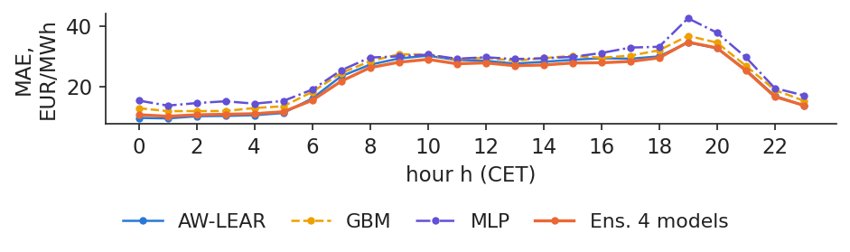
          The chart shows the MAE by hour of AW-LEAR, GBM, MLP and the ensemble of 4. Alone, the machine-learning models are better than AW-LEAR in 0 hours (GBM) and 0 hours (MLP). The ensemble of 4, which contains them, is better than AW-LEAR in 15 of the 24 hours. This is the practical meaning of (2.12): a weaker model whose errors are different still improves the average.

          The profile by hour also shows where errors are concentrated. The hardest hour is 19 h CET, the evening ramp, when solar output disappears and demand is still high; there AW-LEAR has MAE 34.52 EUR/MWh. Night and early-morning hours are much easier.

          In practice: put your best analyst on the evening hours, where the money is lost.
          Chart: Accuracy by hour: machine-learning models alone and in the ensemble

          MAE by hour (CET) on the test year for AW-LEAR, GBM, MLP and the ensemble of 4; the ML models are refitted monthly.

          Source: energy-charts.info (Fraunhofer ISE); OPCOM prices; ENTSO-E generation and flows (Transelectrica data for Romania); Yahoo Finance (SparkChange EUA ETC). Data: test year 2025-11-01 to 2026-10-31; ML refitted monthly.

          Research from our group on Romanian load: machine learning is most accurate for smooth series

          Slide 34 in the PDF

          Machine learning is not always behind linear models. A study from our group (Proșcanu, Proșcanu, Pele & Costea, 2025) benchmarked classical seasonal models against neural networks on the hourly national load of Romania for 2022–2024. Case study C2 of the course replicates the comparison under the same gate-closure rule as this lecture: 217 test days from 27 May 2024, with load metered up to \(d-2\).

          In the replication the MAPE is 4.09% for gradient boosting, 4.16% for the Chronos-Bolt foundation model and 4.58% for the MLP, against 4.85% for a linear regression, 8.03% for a seasonal autoregressive model and 10.17% for the naive forecast that copies the load of two days earlier. These C2 figures are computed by the C2 case notebook on our data; the paper's own results are in the case brief.

          The contrast with prices has a clear reason. Load is smooth and never near zero, so MAPE is meaningful and nonlinear models have regular patterns to learn. Prices jump and turn negative; there, a well-built linear model is hard to beat.

          In practice: forecast your own load with ML and the price with LEAR plus an ensemble.

          Section summary

          Averaging across calibration windows and across models gives the best forecasts of the test year: the ensemble of 4 reaches rMAE 0.795. Machine-learning models help inside the ensemble even when they lose alone.

          Probabilistic forecasts and cointegration

          A point forecast is not enough for risk management, and prices of neighbouring markets or of fuels are linked in the long run. This section turns point forecasts into quantiles with QRA and checks their calibration, then tests cointegration between Romania and Hungary and between power, gas and hydro.

          Quantile regression averaging: from point forecasts to quantiles

          Slide 36 in the PDF

          QRA regresses the actual price on several point forecasts, separately for each quantile level, and the point forecasts become a distribution (Koenker & Bassett, 1978; Nowotarski & Weron, 2015):

          \[\hat q^{\tau}_{d,h}=\beta^{\tau}_{0,h}+\beta^{\tau}_{1,h}\hat P^{\text{AW-ARX}}_{d,h}+\beta^{\tau}_{2,h}\hat P^{\text{AW-LEAR}}_{d,h}\]
          (2.16)
          \[\text{PS}_\tau(q,y)=\big(\mathbf{1}\{y<q\}-\tau\big)(q-y)\]
          (2.17)

          where \(\hat q^{\tau}_{d,h}\) is the forecast quantile of level \(\tau\) for hour \(h\) of day \(d\), \(\hat P^{\text{AW-ARX}}_{d,h}\) and \(\hat P^{\text{AW-LEAR}}_{d,h}\) are the two point forecasts, and the coefficients \(\boldsymbol\beta^{\tau}_h=(\beta^{\tau}_{0,h},\beta^{\tau}_{1,h},\beta^{\tau}_{2,h})\) minimise the pinball score (PS) of (2.17) on the last 182 days of forecasts, re-estimated weekly. In (2.17), \(q\) is a quantile forecast, \(y\) the realised price and \(\mathbf{1}\{y<q\}\) equals 1 when the price falls below the quantile and 0 otherwise. The levels are \(\tau=0.01,\dots,0.99\).

          Two simpler methods serve as comparison: conformal prediction (CP) and historical simulation (HS), which both use the AW-LEAR errors of the last 112 days, as in Assignment 1. The average pinball score (lower is better) is 8.33 for QRA, 8.47 for CP and 8.41 for HS. The 90% interval, however, covers only 85.7% of the prices for QRA, 87.0% for CP and 85.8% for HS; the mean width of the QRA interval is 93.0 EUR/MWh. All three are below 90%, and the Kupiec test rejects correct coverage.

          In practice: a 90% band that holds 86% of the prices understates the risk of the open position.

          A week of QRA intervals in Romania: wide in the evening, narrow at night

          Slide 37 in the PDF

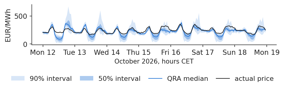
          The chart shows the QRA forecasts for the week 12 Oct 2026 – 18 Oct 2026, hour by hour: the 90% and 50% intervals, the QRA median and the actual price. The band widens where the evening price is uncertain and narrows in the calm night hours. This is what a good probabilistic forecast should do: the width of the interval follows the uncertainty of each hour, instead of being the same every hour.

          The median of the QRA distribution is itself a point forecast. Over the test year it has MAE 22.14 EUR/MWh, as good as the best point forecast. Moving from points to quantiles therefore costs nothing in point accuracy and adds a measure of risk (Nowotarski & Weron, 2015).

          In practice: bid the 50% band for volumes you must buy, the tails for what you can shift.
          Chart: A week of QRA intervals in Romania: wide in the evening, narrow at night

          Hourly actual price, QRA median and 50% and 90% QRA intervals for the week 12–18 Oct 2026, in EUR/MWh.

          Source: energy-charts.info (Fraunhofer ISE); OPCOM prices; ENTSO-E load, wind and solar (Transelectrica data for Romania). Data: week 2026-10-12 to 2026-10-18, hourly.

          All three methods are too narrow in the tails

          Slide 38 in the PDF

          A probabilistic forecast is calibrated when \(\tau\)% of the prices fall below the \(\tau\)-quantile, for every level \(\tau\). The chart plots, for the 99 quantile levels, the coverage error: the actual share of prices below the forecast quantile minus \(\tau\), in percentage points; a calibrated forecast lies on the zero line. All three methods lie above the line on the left and below it on the right: too many prices fall below the low quantiles and above the high ones, so the tails are too narrow.

          The Kupiec test for the 90% interval confirms it formally (Kupiec, 1995; Gneiting & Raftery, 2007). Its statistic is 162.9 for QRA, 83.3 for CP and 154.1 for HS, far above the 5% critical value of 3.84. The test is defined in Appendix C.

          In practice: widen the tails before using quantiles for collateral (Lecture 4).

          Interactive chartInteractive page →

            Code of this chart: EMQA_L2_prob_rel · open in Colab

            Actual share of prices below each forecast quantile minus the quantile level \(\tau\), in percentage points, for QRA, CP and HS over the 99 quantile levels of the test year.

            Source: energy-charts.info (Fraunhofer ISE); OPCOM prices; ENTSO-E load, wind and solar (Transelectrica data for Romania). Data: test year 2025-11-01 to 2026-10-31, 99 quantiles.

            Question for the room The 90% QRA interval (built from the AW-ARX and AW-LEAR forecasts) should contain the price in 90% of the hours. How often does it in the test year?
            Answer

            In 85.67% of the hours, below 90%: the interval is too narrow, and the Kupiec test (a likelihood-ratio test of the share of hours outside the interval) rejects correct coverage (p < 0.001). The 50% interval covers 47.3%. The reliability chart shows, for each quantile level τ, the share of prices below the quantile minus τ, in percentage points (pp): above zero in the lower tail and below zero in the upper tail, so extreme prices are more frequent than the model expects. Choose an hour: the evening hours have the widest intervals.

            Two trending prices are cointegrated when their spread keeps returning

            Slide 39 in the PDF

            Two prices may each wander without a fixed mean, yet a combination of them may be stationary: the gap keeps closing and the regression between them is not spurious. The Engle–Granger procedure tests this in two steps (Engle & Granger, 1987):

            \[P^{\text{RO}}_t=\alpha+\beta P^{\text{HU}}_t+u_t\]
            (2.18)
            \[\Delta\hat u_t=\rho\,\hat u_{t-1}+\textstyle\sum_j\gamma_j\Delta\hat u_{t-j}+\eta_t\]
            (2.19)

            where \(P^{\text{RO}}_t\) and \(P^{\text{HU}}_t\) are the daily prices of Romania and Hungary, \(\alpha\) and \(\beta\) are estimated by OLS in step 1 (2.18), \(\hat u_t\) is the residual (the spread), and step 2 (2.19) tests for a unit root in \(\hat u_t\), with \(\Delta\) the first difference, \(\gamma_j\) the coefficients of the lagged differences and \(\eta_t\) an error. The null hypothesis is no cointegration (\(\rho=0\)), with MacKinnon (1996) critical values. The Johansen trace test (Johansen, 1991) tests instead the rank \(r\), the number of cointegrating relations, of a vector error-correction model.

            For Romania and Hungary, daily since 1 Jan 2022, \(\hat\beta\) = 0.963 and the Engle–Granger statistic is −10.58 against a 5% critical value of −3.34: the prices are cointegrated. A shock to the spread halves in 0.8 days. The Johansen trace test gives 139.7 against 15.49 for \(r=0\) and 6.21 against 3.84 for \(r\le1\), so rank 2: the levels themselves are nearly stationary since 2022 (augmented Dickey–Fuller (ADF) \(p\) = 0.064).

            In practice: a RO–HU spread trade closes within days, not months.

            Romania and Hungary: cointegrated prices in coupled markets

            Slide 40 in the PDF

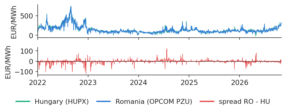
            The upper panel of the chart shows the daily base prices of Romania (OPCOM PZU) and Hungary (HUPX) since 2022; the lower panel shows their spread. The two series are almost indistinguishable at this scale. The spread RO − HU has a mean of −2.07 EUR/MWh and a standard deviation of 15.08. For comparison, the spread between Romania and Germany–Luxembourg has a mean of 21.06 and a standard deviation of 37.79: the farther market is less tightly linked.

            In the test year the Romanian and Hungarian prices were identical in 10.1% of the hours. In the remaining hours the border between the two zones was congested, and the prices could differ, but the gap kept closing (Engle & Granger, 1987).

            In practice: use the Hungarian price as a regressor or a check on your Romanian forecast.
            Chart: Romania and Hungary: cointegrated prices in coupled markets

            Daily base prices of Romania and Hungary from 1 Jan 2022 to 31 Oct 2026 (top) and their spread RO − HU (bottom), in EUR/MWh.

            Source: energy-charts.info (Fraunhofer ISE); prices of OPCOM (RO), HUPX (HU) and EPEX SPOT (DE-LU), via ENTSO-E. Data: daily base prices, 2022-01-01 to 2026-10-31.

            Power, gas and hydro: an error-correction model on monthly data

            Slide 41 in the PDF

            Lecture 1 regressed the monthly Romanian power price on the gas price and on hydro generation. If price and gas are cointegrated, that regression is not spurious, and the price is pulled back each month towards its gas-implied level while hydro moves it in between. The error-correction model (ECM) writes this directly:

            \[\Delta P_t=c+\underbrace{\alpha\,(P_{t-1}-a-\beta\,\text{TTF}_{t-1})}_{\text{error correction}}+\gamma\,\Delta\text{TTF}_t+\delta\,H_t+\varepsilon_t\]
            (2.20)

            where \(P_t\) is the monthly mean price of Romania, \(\text{TTF}_t\) the gas price in EUR/MWh, \(a+\beta\,\text{TTF}_{t-1}\) the long-run (gas-implied) level of the price, \(H_t\) hydro output minus its calendar-month mean in TWh (terawatt-hours), which is stationary, \(c\) a constant, \(\gamma\) the immediate effect of a change in gas, \(\delta\) the effect of extra hydro and \(\varepsilon_t\) the error. The coefficient \(\alpha<0\) is the speed of return to the long-run level.

            On data from 2015-01 to 2026-10, the Engle–Granger statistic is −5.64 against a 5% critical value of −3.38 and the Johansen rank is 1: price and gas are cointegrated. The estimate \(\hat\beta\) = 1.95 means the price behaves as if a gas plant of about 51% efficiency set it. In the ECM, \(\hat\alpha\) = −0.452, which gives a half-life of 1.2 months, and \(\hat\delta\) = −12.80 EUR/MWh per TWh of extra hydro, with \(t\) = −3.10 (Engle & Granger, 1987; Johansen, 1991).

            In practice: a hydro producer in a dry month can expect prices above the gas-implied level for one or two months.

            Power, gas and hydro: the Lecture 1 regression is not spurious

            Slide 42 in the PDF

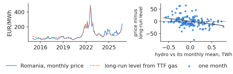
            The left panel of the chart shows the monthly Romanian price together with its long-run level implied by the TTF gas price from the cointegrating regression; the price follows that level, with deviations that close within a few months. The right panel plots, for each month, the deviation of the price from its long-run level against hydro generation relative to its monthly mean. The slope is negative: months with more hydro than usual sit below the gas-implied level, months with less hydro sit above it.

            Together the two panels show that the Lecture 1 regression captures a genuine long-run relation rather than a coincidence of two trending series, and that hydro explains a large part of the temporary deviations.

            In practice: read a dry hydro year as a price premium over gas, not as a new price level.
            Chart: Power, gas and hydro: the Lecture 1 regression is not spurious

            Left: monthly price of Romania and its long-run level from the TTF gas price, 2015-01 to 2026-10, in EUR/MWh; right: deviation from the long-run level against hydro generation minus its monthly mean, in TWh, one dot per month.

            Source: energy-charts.info (OPCOM prices; ENTSO-E hydro generation, Transelectrica data); World Bank Pink Sheet (TTF). Data: monthly, 2015-01 to 2026-10.

            Section summary

            QRA turns point forecasts into intervals whose width follows the uncertainty of each hour, but all methods have tails that are too narrow. Romania and Hungary are cointegrated with a spread that halves in less than a day, and the monthly power price is cointegrated with gas, with hydro explaining the deviations.

            Case studies on recent Romanian data

            Four case studies apply the models of the lecture to recent Romanian data and translate accuracy into the questions a manager asks: how stable the accuracy is over the year, what happens in a stress week, how to forecast the new quarter-hour prices and what a better forecast is worth in euros. The section ends with a checklist for any forecasting desk.

            Case study (a): a year of forecasts, month by month

            Slide 44 in the PDF

            The chart follows the monthly MAE of the naive benchmark, AW-ARX, AW-LEAR and the ensemble of 4 over the test year. AW-LEAR beats naive in 12 of the 12 months, so the gain is not an artefact of one good period. The level of the error, however, varies a lot: the MAE of AW-LEAR ranges from 12.84 EUR/MWh in December 2025 to 34.88 EUR/MWh in October 2026.

            The monthly view also shows that a good annual average can hide weak periods: October 2026 is the hardest month of the test year. The quarterly breakdown in Appendix B tells the same story.

            In practice: report accuracy by month, since a good annual MAE can hide a bad autumn.

            Interactive chartInteractive page →

            Models

              Code of this chart: EMQA_L2_monthly_mae · open in Colab

              Monthly MAE of the naive benchmark, AW-ARX, AW-LEAR and the ensemble of 4 over the test year, in EUR/MWh.

              Source: energy-charts.info (Fraunhofer ISE); OPCOM prices; ENTSO-E generation and flows (Transelectrica data for Romania); Yahoo Finance (SparkChange EUA ETC). Data: test year 2025-11-01 to 2026-10-31.

              Question for the room Is AW-LEAR better than the naive forecast in every month of the test year, and is the ensemble of four models always better than AW-LEAR?
              Answer

              AW-LEAR beats the naive forecast in all 12 months; the ensemble (mean of AW-ARX, AW-LEAR, GBM and MLP) beats AW-LEAR in 8 of the 12 months. The error level moves a lot between months: AW-LEAR has 12.84 EUR/MWh in December 2025 and 34.88 in October 2026. Switch to the relative MAE: the ranking of the models is more stable than the level of their errors.

              Case study (b): the stress week of 19 Oct 2026

              Slide 45 in the PDF

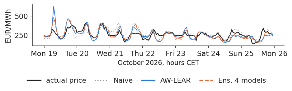
              The week from 19 to 25 Oct 2026 was a period of stress on the Romanian market. The mean price was 258.59 EUR/MWh and the peak 412.35 EUR/MWh. The chart shows the actual hourly price together with the forecasts of the naive benchmark, AW-LEAR and the ensemble.

              In this week the MAE is 40.19 for naive, 36.54 for AW-LEAR, 34.35 for GBM and 34.95 for the ensemble. The models still beat naive, but every one of them lags a sudden jump in the price level by about a day: the forecasts rely on yesterday's prices, so they catch up only once the new level has appeared in the data. GBM, behind AW-LEAR over the whole year, is the best single model in this week.

              In practice: every model lags a jump in level by a day, so hedge the evening hours.
              Chart: Case study (b): the stress week of 19 Oct 2026

              Actual hourly price and the forecasts of the naive benchmark, AW-LEAR and the ensemble for the week 19–25 Oct 2026, in EUR/MWh.

              Source: energy-charts.info (Fraunhofer ISE); OPCOM prices; ENTSO-E generation and flows (Transelectrica data for Romania); Yahoo Finance (SparkChange EUA ETC). Data: week 2026-10-19 to 2026-10-25, hourly.

              Case study (c): forecasting 96 quarter-hours since 1 October 2025

              Slide 46 in the PDF

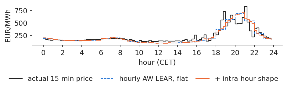
              Since 1 October 2025 the market time unit (MTU) of the day-ahead auction is 15 minutes, so each hour has four prices. The hourly models of this lecture forecast the mean of the four. A simple way to obtain quarter-hour forecasts is to add to the hourly AW-LEAR forecast the mean intra-hour shape of the 28 previous days, that is how much each quarter-hour has typically deviated from its hourly mean.

              The chart shows one day, 1 Jul 2026: the actual 15-minute price, the hourly AW-LEAR forecast kept flat within the hour and the shaped forecast. On the 363 test days without DST, the quarter-hour MAE is 26.02 EUR/MWh with a flat hour and 24.53 EUR/MWh with the shape. A simple profile, estimated only from past days, already recovers part of the structure within the hour.

              In practice: a battery bids per quarter-hour; give it the intra-hour shape, not a flat hour.
              Chart: Case study (c): forecasting 96 quarter-hours since 1 October 2025

              Actual 15-minute prices on 1 Jul 2026, the hourly AW-LEAR forecast kept flat within the hour and the forecast with the intra-hour shape of the 28 previous days, in EUR/MWh.

              Source: energy-charts.info (Fraunhofer ISE); OPCOM 15-minute day-ahead prices for Romania, via ENTSO-E. Data: 2026-07-01, 96 quarter-hours (CET).

              Case study (d): economic value of a more accurate forecast

              Slide 47 in the PDF

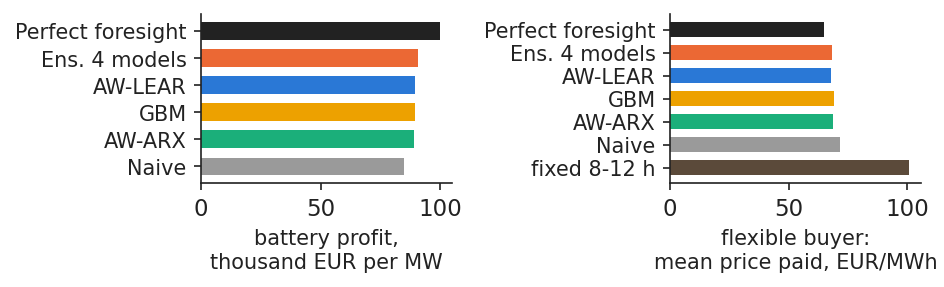
              A better rMAE is useful only if it changes decisions. The case study translates forecast accuracy into money for two users. The first is a battery of 1 MW (megawatt) and 2 MWh with a round-trip efficiency of 90%, which runs one daily cycle, charging in the cheapest hours and discharging in the most expensive ones as chosen from the forecast. Over the 363 days without DST it earns 90,738 EUR per MW with the ensemble forecast, which is 91.0% of the profit under perfect foresight, against 84,623 EUR with the naive forecast.

              The second is a supplier with a flexible process of four hours that can be placed anywhere in the day. Placing it in the hours that AW-LEAR forecasts to be cheapest costs 67.87 EUR/MWh, against 100.59 EUR/MWh for a fixed 8–12 h CET block. The chart shows both results for perfect foresight, the ensemble, AW-LEAR, GBM, AW-ARX and naive.

              In practice: translate rMAE into EUR before paying for a forecast.
              Chart: Case study (d): economic value of a more accurate forecast

              Left: battery profit over the test year in thousand EUR per MW for each forecast and for perfect foresight; right: average price paid by the flexible buyer in EUR/MWh, with the fixed 8–12 h block for comparison.

              Source: energy-charts.info (Fraunhofer ISE); OPCOM prices; ENTSO-E generation and flows (Transelectrica data for Romania); Yahoo Finance (SparkChange EUA ETC). Data: test year 2025-11-01 to 2026-10-31; 1 MW / 2 MWh, round-trip efficiency 90%.

              Forecasting checklist and a test for the use of future information

              Slide 48 in the PDF

              Before trusting a backtest, a forecasting desk should check three things: every input was public before 12:00 CET on \(d-1\); scalers, transformations, the penalty \(\lambda\) and any thresholds were fitted in the calibration window only; and validation was chronological, with the test year touched once. Then the report should give the MAE and rMAE against naive, the DM p-values and the coverage of the intervals, by month and by hour, not only one annual number.

              The analysis behind this lecture checks itself for leakage of future information (analysis script, section 7). It runs 9,364 timestamp checks, verifying that each input was available at least 12 h before the cut-off. It recomputes 17 forecast series on 14 days, and GBM and MLP on the first day of all 12 refits, after deleting all later data or replacing it with nonsense; the forecasts stay identical up to rounding. Status: passed (Lago et al., 2021).

              In practice: make the leakage check part of every model review, as Assignment 1 does.

              AIDA 2026: economic evaluation of probabilistic forecasts

              Slide 49 in the PDF

              Two talks at the AIDA 2026 conference (Bucharest University of Economic Studies, June 2026) connect this lecture to current research; the findings and numbers below are those printed on the conference slides.

              • R. Weron, keynote, 4 June 2026 (slides). Price models are either one model per hour, as our ARX and LEAR, or a joint model of all 24 hours; averaging across calibration windows and LEAR remain the benchmarks every new model must beat. Trading on quantiles earned 19–34% more than trading on point forecasts (Uniejewski & Weron, 2021). In a 2021–2025 test, the pretrained transformer TabPFN 3.0 reached a continuous ranked probability score (CRPS) of 3.56 in 2025, against 4.71 for LEAR with conformal intervals.
              • A. Petukhina, with G. Mazzon and D. Marazzina, 3 June 2026 (slides). Great Britain, outside SDAC, runs two hourly day-ahead auctions (EPEX SPOT and Nord Pool), so a trader can buy in one and sell in the other. The work forecasts the joint distribution of both auction prices and the system price with a copula model and tests it from March to September 2022. On the EPEX auction its MAE is 47.884 against 27.926 for LASSO with QRA, but its CRPS is 16.852 against 32.605; trading on the mean and the conditional value at risk (CVaR), it ends with 22,001 EUR, against 6,283.3 and −3,005.1 EUR for the two LASSO-based benchmarks. The work builds on Agakishiev et al. (2025).
              In practice: judge a forecast by the decision it feeds: in Great Britain the model with the larger MAE earned more.

              AIDA 2026: a data-driven merit order forecasts the price distribution

              Slide 50 in the PDF
              • P. Ghelasi, with J. Browell and F. Ziel, 3 June 2026 (slides). The price is where the merit order, the power plants sorted by variable cost, meets the load: a fundamental model that can be read plant by plant. Instead of fixing plant efficiencies and CO₂ intensities from expert tables, the model estimates them from past prices, within expert bounds (Ghelasi & Ziel, 2026). On German data, trained from 1 October 2022 to 1 October 2023 and tested to 1 October 2024 without recalibration, its MAE is 11.83 EUR/MWh, against 13.11 for LASSO, 13.96 for boosted trees, 16.36 for the classical merit order and 24.96 for the naive model. The probabilistic version forecasts the distribution of each input (load, solar, wind, fuels), passes every sampled scenario through the merit order and chooses the parameters that minimise the CRPS of the resulting prices. Its CRPS is 13.92, against 14.04 for a model with the Johnson \(S_U\) distribution and 20.46 for the naive model, and the simulated prices form non-parametric distributions, for example a cluster near zero at midday.
              In practice: a fundamental model estimated statistically gives forecasts you can explain plant by plant.

              Section summary

              Accuracy varies strongly by month and every model lags a sudden jump in level by a day, but better forecasts translate into money: the ensemble earns a battery 91.0% of the perfect-foresight profit. A checklist and a leakage self-check make the results credible.

              Wrap-up

              The wrap-up tests the main ideas with five short questions, summarises the lecture and lists the research of our group and further reading.

              Self-assessment questions

              Slide 51 in the PDF
              1. It is Sunday, 11:30 CET, and you must forecast Monday at 19:00 with the naive benchmark. Which price do you use?
                Answer: the price of the previous Monday at 19:00 (\(d-7\)). On our test year this beats the most recent price on Mondays, Saturdays and Sundays (MAE 29.87 against 33.48 EUR/MWh).
              2. A vendor reports rMAE 0.55 for Romania and uses the realised load of day \(d-1\) as a regressor. Do you buy?
                Answer: no. At 12:00 on \(d-1\) that day is not yet metered, so the backtest leaks information. Ask for a rerun with data up to \(d-2\) (or with published day-ahead forecasts); our honest best is rMAE 0.795.
              3. AW-ARX or AW-LEAR? The DM test gives \(p\) = 0.797. Which model goes into production?
                Answer: neither wins significantly. Take the simpler one or, better, their average, which is part of the best ensemble (rMAE 0.795).
              4. Your report shows a MAPE of 5,778% for the Romanian price forecast and the board is alarmed. What do you say?
                Answer: MAPE divides by prices near zero; 387 hours below 5 EUR/MWh produce 99.5% of it. Report MAE 22.53 EUR/MWh and rMAE 0.810 instead.
              5. The RO–HU spread is cointegrated with a half-life of 0.8 days, and today Romania is 40 EUR/MWh above Hungary. What do you expect?
                Answer: the gap should shrink by about half within a day, unless the border stays congested. It is a signal for cross-border trading, not a guarantee.

              The lecture started with an honest setup: only information available at 12:00 CET on \(d-1\), rolling calibration windows, the naive benchmark and DM tests to compare models. On that basis, expert ARX models and their LASSO version LEAR cut the naive error by almost a fifth, and averaging across windows and models adds a further, statistically significant gain. On the test year the best model, an ensemble of 4, cuts the naive error by 20.5%.

              QRA turns these point forecasts into intervals, which are useful but too narrow in the tails. Cointegration links the Romanian price to the Hungarian one and, in the long run, to gas. The next lecture turns from the level of prices to their volatility (Lecture 3).

              Research from our group on forecasting Romanian power

              Slide 57 in the PDF

              Several papers from our group at the Bucharest University of Economic Studies and the Romanian Academy, Institute for Economic Forecasting, address the questions of this lecture. The findings below are those stated in the papers; the numbers on the other slides come from our own data.

              • Benchmarking load forecasts. Proșcanu, Proșcanu, Pele & Costea (2025) compare classical seasonal models with neural networks on Romania's national electricity consumption; in the paper a neural network has a clearly lower error than the seasonal autoregressive benchmark. The comparison is the basis of case study C2.
              • Four generations of price models. Andrei, Velev, Toma, Pele & Lessmann (2024) carry out a comparative evaluation of four generations of forecasting methods for energy prices, a reference for choosing a model family.
              • Explaining price forecasts across horizons. Andrei, Pele & Cramer (2026) show which drivers matter at which forecast horizon and in which price regime for Romanian hourly prices.
              • Early warning of price spikes. Andrei, Pele, Cramer, Amza & Diaconu (2026) build an explainable artificial intelligence (AI) system for the Romanian market in which the previous price and the residual load drive the spikes, a preview of Lecture 7.

              Further reading and resources

              Slide 58 in the PDF
              • R. Weron, IIF Distinguished Lectures on electricity price forecasting (2025): slides part I, part II and notebooks.
              • epftoolbox, with LEAR and DNN and the open benchmark of Lago et al. (2021): github.com/jeslago/epftoolbox.
              • Forecasting: Principles and Practice, 3rd edition: otexts.com/fpp3.
              • This course, with code, data and notebooks: github.com/danpele/EMQA. The notebook of this lecture reproduces every chart and number.
              • Assignment 1 applies ARX, LEAR, the DM test and the HS and CP intervals to your own test window.

              Appendix

              The appendix gives the technical details behind the main slides: the full specification of LEAR, the accuracy by quarter, the probabilistic scores with the Kupiec test, and all unit-root and cointegration tests.

              Appendix A: LEAR in full

              Slide 63 in the PDF

              The penalty \(\lambda\) of (2.10) is chosen every day by the AIC computed along the LASSO path:

              \[\text{AIC}(\lambda)=n\ln\frac{\text{RSS}(\lambda)}{n}+2\,\mathrm{df}(\lambda)\]
              (2.21)

              where \(n\) is the number of calibration days, \(\text{RSS}(\lambda)\) the residual sum of squares (RSS) of the fit with penalty \(\lambda\) and \(\mathrm{df}(\lambda)\) the degrees of freedom, equal to the number of non-zero coefficients. The path is computed by least angle regression (LARS), in scikit-learn.

              The price block is transformed with (2.9), where \(m\) and \(s\) are the median and 1.4826 · MAD of the prices of rows \(d-T-7,\dots,d-1\), pooled over the 24 hours. Load and wind + solar have their own asinh transformation from rows up to \(d-2\), and then every column is z-scored on the calibration rows. The 247 columns are made up as follows:

              BlockColumns
              prices d-1, all 24 hours24
              prices d-2, d-3, d-772
              load d-2, d-3, d-772
              wind + solar d-2, d-3, d-772
              day of week7
              total247

              Appendix B: MAE by quarter of the test year

              Slide 64 in the PDF

              The table gives the MAE, in EUR/MWh, of the main models by quarter. The test year starts on 1 Nov 2025, so the quarters have 61, 90, 91, 92 and 31 days. On the slide green marks the best model in each quarter and red the worst.

              Model2025 Q42026 Q12026 Q22026 Q32026 Q4
              naive19.8030.1927.5528.3236.05
              AW-ARX15.2423.6222.9722.0931.05
              AW-LEAR14.8622.9922.6422.9134.88
              GBM16.2524.7122.9824.9737.88
              MLP17.2725.4924.8926.3041.58
              ensemble of 414.8223.0222.0922.5032.91

              The ensemble is the best or close to the best in every quarter, while the ranking of the single models changes; in the last month, October 2026, AW-ARX does better than AW-LEAR.

              Appendix C: probabilistic scores and the Kupiec test

              Slide 65 in the PDF

              The Kupiec test (Kupiec, 1995) is a likelihood ratio (LR) test of unconditional coverage (UC):

              \[\text{LR}_{\text{UC}}=-2\ln\frac{(1-p_0)^{n-x}p_0^{\,x}}{(1-\hat p)^{n-x}\hat p^{\,x}}\sim\chi^2_1,\qquad \hat p=\frac xn\]
              (2.22)

              where \(x\) is the number of hours outside the 90% interval, \(n\) = 8,760 the number of hours, \(p_0=0.10\) the nominal share outside the interval and \(\hat p\) the observed share; under correct coverage the statistic follows a \(\chi^2\) distribution with one degree of freedom. Hours of the same day are not independent, so the test is indicative; a test on the daily share of misses with Newey–West variance gives \(p<0.001\) for QRA.

              The pinball score is averaged over the 99 quantiles; the continuous ranked probability score is approximately 2 × this score (Gneiting & Raftery, 2007).

              MethodPinballCov. 50%Cov. 90%Kupiec
              QRA8.3347.385.7162.9
              CP8.4746.587.083.3
              HS8.4145.885.8154.1

              Appendix D: unit-root and cointegration tests in full

              Slide 66 in the PDF

              The table lists all unit-root and cointegration tests of the lecture. ADF tests use lags chosen by the AIC; the Johansen tests include a constant and 6 lagged differences for daily data or 2 for monthly data. The ECM of (2.20) is estimated with heteroskedasticity- and autocorrelation-robust standard errors (6 lags) on 141 months, with \(R^2\) = 0.778.

              Series / pairTestStatisticp / crit. 5%
              RO, HU, DE-LU daily levelsADF p–0.064, 0.052, 0.015
              RO–HUEngle–Granger−10.58−3.34
              RO–HUJohansen r=0 / r≤1139.7 / 6.2115.49 / 3.84
              RO–DE-LUEngle–Granger−5.79−3.34
              RO price, TTF, monthly levelsADF p–0.295, 0.249
              hydro minus monthly meanADF p–0.002
              price–TTFEngle–Granger−5.64−3.38
              price–TTF–hydroEngle–Granger−5.95−3.80
              price–TTFJohansen r=0 / r≤121.32 / 3.7415.49 / 3.84

              The monthly price and TTF levels have unit roots (ADF p-values 0.295 and 0.249), while hydro minus its monthly mean is stationary (0.002); the Engle–Granger tests reject no cointegration for every pair, which supports the ECM of (2.20).

              Abbreviations

              ADFaugmented Dickey–Fuller test
              AIartificial intelligence
              AICAkaike information criterion
              ARXautoregressive model with exogenous variables
              AWaveraging across calibration windows
              AW-ARXARX averaged across calibration windows
              AW-LEARLEAR averaged across calibration windows
              CETCentral European Time
              CPconformal prediction
              CRPScontinuous ranked probability score
              CVaRconditional value at risk
              DE-LUGermany–Luxembourg bidding zone
              DMDiebold–Mariano test
              DNNdeep neural network
              DSTdaylight saving time
              ECMerror-correction model
              ENTSO-EEuropean Network of Transmission System Operators for Electricity
              EPEXEPEX SPOT power exchange
              ETCexchange-traded commodity
              EUEuropean Union
              EUAEU emission allowance (1 t CO_2)
              EUPHEMIAPan-European Hybrid Electricity Market Integration Algorithm
              EUReuro
              GBMgradient boosting machine (boosted trees)
              HShistorical simulation
              HUHungary (bidding zone)
              HUPXHungarian Power Exchange
              ISEFraunhofer Institute for Solar Energy Systems
              LARSleast angle regression
              LASSOleast absolute shrinkage and selection operator
              LEARLASSO-estimated autoregression
              LRlikelihood ratio
              MADmedian absolute deviation
              MAEmean absolute error
              MAPEmean absolute percentage error
              MLmachine learning
              MLPmultilayer perceptron (feed-forward neural network)
              MTUmarket time unit
              MWmegawatt
              MWhmegawatt-hour
              OLSordinary least squares
              OPCOMRomanian electricity and gas market operator
              PSpinball score
              PZUPiața pentru Ziua Următoare (day-ahead market)
              QRAquantile regression averaging
              ReLUrectified linear unit
              rMAErelative MAE (model MAE / naive MAE)
              RMSEroot mean squared error
              RORomania (bidding zone)
              RSSresidual sum of squares
              SDACSingle Day-Ahead Coupling
              sMAPEsymmetric MAPE
              TSOtransmission system operator
              TTFTitle Transfer Facility (Dutch gas hub)
              TWhterawatt-hour
              UCunconditional coverage
              VSTvariance-stabilising transformation

              References

              • Andrei, A.-V., Pele, D.-T. & Cramer, A.-A. (2026). Multi-horizon explainability in energy price forecasting: Disentangling market dynamics and renewable intermittency in Romania's liberalized electricity market. Proceedings of the International Conference on Business Excellence, 20(1), 104–117. doi:10.2478/picbe-2026-0014
              • Andrei, A.-V., Pele, D.-T., Cramer, A.-A., Amza, A. & Diaconu, D. (2026). Explainable AI-based early warning system for electricity price spikes: Evidence from the Romanian market. Proceedings of the International Conference on Business Excellence, 20(1), 4820–4836. doi:10.2478/picbe-2026-0352
              • Andrei, A.-V., Velev, G., Toma, F.-M., Pele, D. T. & Lessmann, S. (2024). Energy price modelling: A comparative evaluation of four generations of forecasting methods. arXiv:2411.03372. arxiv.org/abs/2411.03372
              • Agakishiev, I., Härdle, W. K., Kopa, M., Kozmík, K. & Petukhina, A. (2025). Multivariate probabilistic forecasting of electricity prices with trading applications. Energy Economics, 141, 108008. doi:10.1016/j.eneco.2024.108008
              • Bates, J. M. & Granger, C. W. J. (1969). The combination of forecasts. Operational Research Quarterly, 20(4), 451–468. doi:10.1057/jors.1969.103
              • Diebold, F. X. & Mariano, R. S. (1995). Comparing predictive accuracy. Journal of Business & Economic Statistics, 13(3), 253–263. doi:10.1080/07350015.1995.10524599
              • Engle, R. F. & Granger, C. W. J. (1987). Co-integration and error correction: Representation, estimation, and testing. Econometrica, 55(2), 251–276. doi:10.2307/1913236
              • Friedman, J. H. (2001). Greedy function approximation: A gradient boosting machine. Annals of Statistics, 29(5), 1189–1232. doi:10.1214/aos/1013203451
              • Ghelasi, P., Browell, J. & Ziel, F. (2026). A probabilistic merit order for electricity price forecasting. AIDA Conference, Bucharest University of Economic Studies, 3 June 2026. github.com/danpele/EMQA/resources/aida2026
              • Ghelasi, P. & Ziel, F. (2026). A data-driven merit order: Learning a fundamental electricity price model. Energy Economics, 154, 109114. doi:10.1016/j.eneco.2025.109114
              • Gneiting, T. & Raftery, A. E. (2007). Strictly proper scoring rules, prediction, and estimation. Journal of the American Statistical Association, 102(477), 359–378. doi:10.1198/016214506000001437
              • Hubicka, K., Marcjasz, G. & Weron, R. (2019). A note on averaging day-ahead electricity price forecasts across calibration windows. IEEE Transactions on Sustainable Energy, 10(1), 321–323. doi:10.1109/TSTE.2018.2869557
              • Hyndman, R. J. & Koehler, A. B. (2006). Another look at measures of forecast accuracy. International Journal of Forecasting, 22(4), 679–688. doi:10.1016/j.ijforecast.2006.03.001
              • Johansen, S. (1991). Estimation and hypothesis testing of cointegration vectors in Gaussian vector autoregressive models. Econometrica, 59(6), 1551–1580. doi:10.2307/2938278
              • Koenker, R. & Bassett, G. (1978). Regression quantiles. Econometrica, 46(1), 33–50. doi:10.2307/1913643
              • Kupiec, P. H. (1995). Techniques for verifying the accuracy of risk measurement models. Journal of Derivatives, 3(2), 73–84. doi:10.3905/jod.1995.407942
              • Lago, J., Marcjasz, G., De Schutter, B. & Weron, R. (2021). Forecasting day-ahead electricity prices: A review of state-of-the-art algorithms, best practices and an open-access benchmark. Applied Energy, 293, 116983. doi:10.1016/j.apenergy.2021.116983
              • NEMO Committee (2025). 15-Minute MTU in SDAC was implemented. SDAC press release, 1 October 2025. nemo-committee.eu
              • NEMO Committee (2026). Single Day-Ahead Coupling (SDAC) and the EUPHEMIA algorithm. nemo-committee.eu/sdac
              • MacKinnon, J. G. (1996). Numerical distribution functions for unit root and cointegration tests. Journal of Applied Econometrics, 11(6), 601–618. doi:10.1002/(SICI)1099-1255(199611)11:6601::AID-JAE4173.0.CO;2-T
              • Marcjasz, G., Serafin, T. & Weron, R. (2018). Selection of calibration windows for day-ahead electricity price forecasting. Energies, 11(9), 2364. doi:10.3390/en11092364
              • Mazzon, G., Petukhina, A. & Marazzina, D. (2026). Multivariate probabilistic day-ahead electricity price forecasting and cross-auction trading in the UK market. AIDA Conference, Bucharest University of Economic Studies, 3 June 2026. github.com/danpele/EMQA/resources/aida2026
              • Nogales, F. J., Contreras, J., Conejo, A. J. & Espínola, R. (2002). Forecasting next-day electricity prices by time series models. IEEE Transactions on Power Systems, 17(2), 342–348. doi:10.1109/TPWRS.2002.1007902
              • Nowotarski, J. & Weron, R. (2015). Computing electricity spot price prediction intervals using quantile regression and forecast averaging. Computational Statistics, 30(3), 791–803. doi:10.1007/s00180-014-0523-0
              • Nowotarski, J. & Weron, R. (2018). Recent advances in electricity price forecasting: A review of probabilistic forecasting. Renewable and Sustainable Energy Reviews, 81, 1548–1568. doi:10.1016/j.rser.2017.05.234
              • Proșcanu, C. A., Proșcanu, M. E., Pele, D. T. & Costea, A. (2025). Watt's next? Benchmarking time series models on Romania's national electricity consumption. Romanian Journal of Economic Forecasting, 28(3), 146–163. RePEc.
              • Tibshirani, R. (1996). Regression shrinkage and selection via the lasso. Journal of the Royal Statistical Society B, 58(1), 267–288. doi:10.1111/j.2517-6161.1996.tb02080.x
              • Uniejewski, B., Nowotarski, J. & Weron, R. (2016). Automated variable selection and shrinkage for day-ahead electricity price forecasting. Energies, 9(8), 621. doi:10.3390/en9080621
              • Uniejewski, B., Weron, R. & Ziel, F. (2018). Variance stabilizing transformations for electricity spot price forecasting. IEEE Transactions on Power Systems, 33(2), 2219–2229. doi:10.1109/TPWRS.2017.2734563
              • Uniejewski, B. & Weron, R. (2021). Regularized quantile regression averaging for probabilistic electricity price forecasting. Energy Economics, 95, 105121. doi:10.1016/j.eneco.2021.105121
              • Weron, R. (2014). Electricity price forecasting: A review of the state-of-the-art with a look into the future. International Journal of Forecasting, 30(4), 1030–1081. doi:10.1016/j.ijforecast.2014.08.008
              • Weron, R. (2026). Machine learning for electricity price forecasting. Keynote, AIDA Conference, Bucharest University of Economic Studies, 4 June 2026. github.com/danpele/EMQA/resources/aida2026
              • Ziel, F. & Weron, R. (2018). Day-ahead electricity price forecasting with high-dimensional structures: Univariate vs. multivariate modeling frameworks. Energy Economics, 70, 396–420. doi:10.1016/j.eneco.2017.12.016

              Text written for the web version of the lecture; numbers, charts and sources come from the slides and their Quantlets.