
Energy Markets Quantitative Analysis

Lecture 6: Renewables and Storage: Cannibalisation, Negative Prices and Batteries

Lecture 6

Renewables and Storage: Cannibalisation, Negative Prices and Batteries

Prof. dr. Daniel Traian PELE

Bucharest University of Economic Studies, Department of Statistics and Econometrics
Romanian Academy, Institute for Economic Forecasting

Solar and wind plants offer their output at a price close to zero, because sunshine and wind cost nothing. Every new park therefore pushes dearer plants out of the market and lowers the price in the hours in which it produces, which are exactly the hours in which every other park of the same technology also produces. This lecture asks what that does to the revenue of a solar park, why prices on the Romanian day-ahead market, Piața pentru Ziua Următoare (PZU), now regularly fall below zero at midday, and how much a battery that buys cheap midday energy and sells it in the evening can actually earn.

The questions matter to every player in the Romanian market: to a solar or wind developer and the bank that finances it, to a supplier or industrial consumer that buys on the PZU, to a battery developer sizing its investment, and to the transmission system operator Transelectrica, which manages the interconnectors. Installed solar capacity in Romania grew 2.4 times from 2019 to 2025, and in 2025 a solar megawatt-hour (MWh) earned only 59.4% of the average price of the year.

All numbers come from real, downloaded data: hourly and 15-minute day-ahead prices for Romania and three neighbouring or reference markets, solar, wind and battery output, the real supply and demand curves of the Romanian market operator, and installed capacity, from 2019 to 31 Oct 2026.

Learning outcomes

  • Measure how much zero-cost solar and wind lower the PZU price, both on the real order book and with a regression on hourly data.
  • Compute the capture price and the capture rate of solar and wind, and explain cannibalisation: the more solar is built, the lower the price it earns.
  • Count negative prices correctly in hour-equivalents, value switching a park off, and read the 15-minute daily price profile.
  • Estimate the arbitrage revenue of 1-, 2- and 4-hour batteries with a linear programme (LP), with perfect foresight and with forecast rules, on hourly and 15-minute prices, in Romania and its neighbours.

Lecture plan

  1. Renewables and the merit orderThis section measures how much solar and wind lower the Romanian day-ahead price, first on the real supply and demand curves of one day and then with a regression on almost four years of hourly data.
  2. Capture prices and cannibalisationA solar park is not paid the average price of the year but the price of the hours in which it produces.
  3. Negative pricesSince 2023, the Romanian day-ahead price sometimes falls below zero.
  4. Intraday shape and price spreadsLow midday prices and high evening prices create a daily price shape.
  5. The economics of a batteryThe daily spread is only a first measure.
  6. Case studies: Apr 2026 and summer 2026Two case studies apply the tools of the lecture to real episodes: April 2026, the month with the most negative hours, and summer 2026, when Romania exported at midday and imported from Bulgaria in the evening.
  7. Wrap-upThe wrap-up checks the main ideas with four questions, summarises the lecture, presents related research from our group and lists resources for further study.
  8. AppendixThe appendix gives the derivations and computational details behind the capture rate, the battery programme, the recomputation of the clearing price and the annuity factor.

Renewables and the merit order

This section measures how much solar and wind lower the Romanian day-ahead price, first on the real supply and demand curves of one day and then with a regression on almost four years of hourly data. It starts with the growth of solar capacity that makes the question urgent.

Data sources: prices, generation, order books and installed capacity

Slide 4 in the PDF

The lecture uses only real data. Day-ahead prices come for four bidding zones: Romania (RO), Bulgaria (BG), Hungary (HU) and the Germany–Luxembourg zone (DE-LU). They are set by the Romanian electricity and gas market operator (OPCOM), the Independent Bulgarian Energy Exchange (IBEX), the Hungarian Power Exchange (HUPX) and the EPEX SPOT power exchange (EPEX), and are taken through energy-charts.info, the data portal of the Fraunhofer Institute for Solar Energy Systems (ISE). Prices are hourly, and every 15 minutes from 1 Oct 2025.

Solar, wind and battery output and electricity consumption (load) come from the European Network of Transmission System Operators for Electricity (ENTSO-E), with Transelectrica as the data provider for Romania; they are available every 15 minutes for Romania and Hungary and hourly for Bulgaria. The real supply and demand curves of the PZU for two quarter-hours come from OPCOM as Extensible Markup Language (XML) files, and installed capacity is yearly, from ENTSO-E through energy-charts.info.

The period runs from 2019 to 31 Oct 2026, the last complete month. On this page "2026" means Jan–Oct 2026, and "the last 12 months" means Nov 2025 – Oct 2026. Delivery days are defined in Central European Time (CET). Energy is always the mean power in megawatts (MW) multiplied by the duration, so a 15-minute market time unit (MTU) counts 0.25 h.
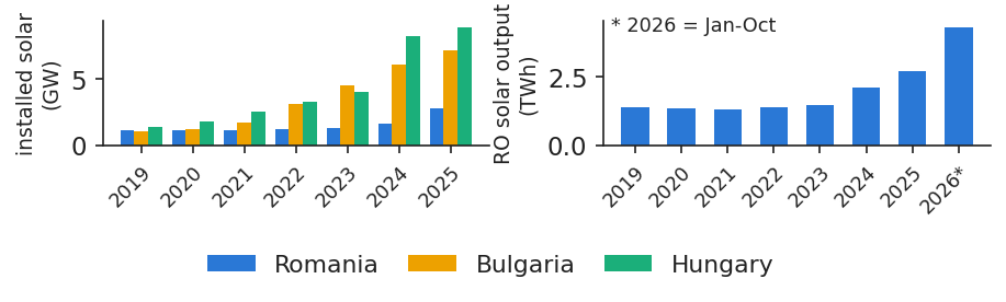

Installed solar in Romania grew 2.4 times from 2019 to 2025

Slide 6 in the PDF

Installed solar capacity in Romania rose from 1.16 gigawatts (GW) at the end of 2019 to 2.79 GW at the end of 2025, 2.4 times more. Output followed: from January to October, Romanian solar plants produced 2.53 terawatt-hours (TWh) in 2025 and 4.32 TWh in 2026. Measured against consumption, solar covered 2.3% of load in 2019 and 10.2% in 2026.

The neighbours grew even faster. At the end of 2025, Bulgaria had 7.2 GW of solar and Hungary 9.0 GW, both much more than Romania. Because the three markets are coupled, this regional capacity matters for Romanian prices as much as the Romanian parks themselves. The output measured by ENTSO-E may omit rooftop panels, so the true amount of solar energy is somewhat larger.

In practice: a new solar park sells in the same sunny hours as every park already built, here and next door.
Chart: Installed solar in Romania grew 2.4 times from 2019 to 2025

Installed solar capacity at year end in Romania, Bulgaria and Hungary, 2019–2025, and Romanian solar output.

Source: energy-charts.info (Fraunhofer ISE), installed capacity from ENTSO-E; ENTSO-E solar output (Transelectrica data). Data: installed capacity at year end 2019-2025; output 2019 to 2026-10-31.

Zero-cost supply shifts the supply curve right and lowers the clearing price

Slide 7 in the PDF

On the day-ahead market, the price of each quarter-hour is set where the supply curve crosses the demand curve. Solar and wind offer near zero, so adding them moves every dearer offer to the right, and the crossing with demand slides down. This is the merit-order effect (Sensfuß, Ragwitz & Genoese, 2008). Formally, if \(X\) extra megawatts are offered at zero, the new clearing price \(p^*(X)\) solves

\[S(p)+X\cdot\mathbf 1[p\ge 0]=D(p)\ \Rightarrow\ p^*(X)\]
(6.1)

and its sensitivity to \(X\) is

\[\frac{\mathrm dp^*}{\mathrm dX}=-\frac{1}{S'(p^*)-D'(p^*)}\]
(6.2)

where \(S(p)\) is the quantity in MW offered at prices up to \(p\), \(D(p)\) the quantity bid at prices of at least \(p\), \(X\) the extra MW offered at 0 EUR/MWh (euro, EUR, per megawatt-hour), \(\mathbf 1[p\ge 0]\) equals one when the price is non-negative and zero otherwise, and \(S'\) and \(D'\) are the slopes of the two curves, in MW per EUR/MWh.

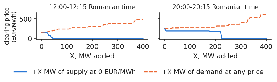
Equation (6.2) says that the effect depends on the shape of the curves near the price. If the curves are flat, many offers sit close to the price and a new park barely moves it; if they are steep, a small extra volume moves the price a lot. On OPCOM's curves for 21 Oct 2026, 12:00–12:15, the price was 152.23 EUR/MWh, and only 34 MW were offered between 1 EUR/MWh and that price: the curve was very steep.

In practice: the steeper the local curve, the more a new park moves its own price.

Romanian order book: 40 MW more at zero price lowers the midday price below 50 EUR/MWh

Slide 8 in the PDF

The chart applies (6.1) to the real curves of 21 Oct 2026. At midday, adding only 25 MW at zero price lowers the price from 152.23 to 131.40 EUR/MWh, and 40 MW push it below 50 EUR/MWh. In the evening the same fall requires 225 MW, because 1,054 MW of net imports make the curve deeper.

These numbers must be read as an upper bound. The recomputation holds cross-border flows, block orders and hourly orders at their accepted values (Appendix C). In the real coupled market, part of any extra midday output is exported, so the Romanian price falls by less. The exercise shows how thin the purely local midday order book is, and why the interconnectors matter.

In practice: for Transelectrica: interconnectors, not local plants, give the midday price its depth.
Chart: Romanian order book: 40 MW more at zero price lowers the midday price below 50 EUR/MWh

Clearing price recomputed on the PZU curves of 21 Oct 2026 against the MW added, as supply at 0 EUR/MWh or as demand at any price, at midday (12:00–12:15) and in the evening.

Source: OPCOM, PZU aggregated curves (XML), own computation. Data: delivery day 2026-10-21; cross-border flows, blocks and hourly orders held at their accepted values.

In the coupled market, 1 GW more solar lowers the Romanian price by about 27 EUR/MWh

Slide 9 in the PDF

To measure the effect in the real coupled market, the lecture estimates a regression on hourly data. Within the same month, clock hour and weekday, sunnier and windier hours are cheaper; the regression measures by how much:

\[P_t=\underbrace{\alpha_{m(t)}+\gamma_{h(t)}+\delta_{w(t)}}_{\text{fixed effects}}+\beta_L L_t+\beta_W W_t+\beta_S S_t+\varepsilon_t\]
(6.3)

where \(P_t\) is the hourly price in EUR/MWh, \(L_t\), \(W_t\) and \(S_t\) are load, wind output and solar output in GW, \(\alpha_{m(t)}\) is a constant for the month of hour \(t\) (it absorbs fuel and carbon prices), \(\gamma_{h(t)}\) a constant for the clock hour, \(\delta_{w(t)}\) a constant for the weekday and \(\varepsilon_t\) the error. The model is estimated by ordinary least squares (OLS).

On 33,600 hours from 2023 to Oct 2026 the fit is \(R^2\) = 0.65. Each GW of solar lowers the price by 26.7 EUR/MWh, each GW of wind by 15.3, and each GW of load raises it by 40.7. The standard error (SE) of the solar coefficient is 2.2, computed to be heteroskedasticity- and autocorrelation-consistent (HAC). At midday in 2026 the mean solar output was 1.62 GW, which corresponds to a price lower by 43.3 EUR/MWh. This is an association, not a causal effect: the regression controls for the calendar, not for everything that moves with sunshine (Cludius et al., 2014; Würzburg et al., 2013).

In practice: a supplier buying midday blocks should expect them cheaper on sunny days, by about this amount.

Price rises with residual load; hours below 2 GW of residual load reached 9.0% in 2026

Slide 10 in the PDF

Residual load is load minus wind minus solar, \(L_t-W_t-S_t\): the demand left for the other plants and for imports. It summarises in one number what the renewables leave to the rest of the system. With the same fixed effects as in (6.3), one more GW of residual load raises the price by 28.3 EUR/MWh (SE 0.9).

The chart groups hours by residual load in bins of 0.5 GW and shows the mean price of each bin. The curve rises steeply: hours with low residual load are cheap, hours with high residual load are dear. What has changed is how often the left end of the curve is reached. Hours with residual load below 2 GW were 0.1% of all hours in 2023 and 9.0% in 2026.

In practice: a hydro producer saves water for high residual load, where each GW is worth most.

Interactive chartInteractive page →

Years

    Code of this chart: EMQA_L6_resid_price · open in Colab

    Mean hourly price by residual load (bins of 0.5 GW with at least 20 hours), 2023 to Oct 2026, by year.

    Source: energy-charts.info (Fraunhofer ISE); OPCOM prices; ENTSO-E solar, wind and load (Transelectrica data for Romania). Data: hourly, 2023-01-01 to 2026-10-31; bins of 0.5 GW with at least 20 hours.

    Question for the room Residual load is load minus wind and solar output. In 2026, how often is the hourly residual load of Romania below 2 GW, and what is the mean price in those hours?
    Answer

    In about 9% of the hours of 2026 (to the cut-off), against 0.1% in 2023; the mean price in those hours is about 51 EUR/MWh, against about 192 EUR/MWh when residual load is above 6 GW. Across 2023–2026, a regression with month, hour and weekday fixed effects gives +28.32 EUR/MWh per GW of residual load (t = 32.1). The cloud of points is wide: residual load explains a large part of the price, but neighbouring markets, hydro and fuel prices move it too.

    Research from our group: machine learning forecasts German redispatch one day ahead

    Slide 11 in the PDF

    Renewables also strain the grid. In Germany the wind blows mostly in the north, while the heaviest demand is in the industrial south. After the day-ahead market has cleared, the four transmission system operators check where lines would be overloaded and order some plants to raise and others to lower their output. This redispatch keeps the grid within its limits; its cost is reimbursed after the fact and does not appear in the day-ahead price.

    A study of our group, presented by Vlad Bolovăneanu at the AIDA 2026 conference (Basangova, Bolovăneanu, Conda, Erlwein-Sayer, Melzer, Pele, Petukhina & Phan, 2026, slides), forecast the hourly redispatch volume in MW, upwards and downwards, of each of the four German operators, 24 hours ahead and with only the information available on the afternoon of the day before: wind, solar, load, price spreads and scheduled cross-border exchanges. The data run from October 2021 to February 2026, and the models were tested on 11 monthly windows from March 2025 to February 2026, comparing statistical, tree-based and deep neural forecasters.

    Deep neural networks were most often among the best models: the best of them is in the model confidence set for the mean absolute error in 6 of the 8 series (4 operators × 2 directions). The explanatory variables help only when they are correctly aligned in time: with all covariates, the forecasts are significantly better in 40–60% of the dense series than without them or with the covariates shifted in time.

    In practice: for Transelectrica: forecast where wind and solar will meet the limits of the grid, a day ahead.

    Section summary

    Zero-cost renewables shift the supply curve and lower the price: on the coupled market by about 27 EUR/MWh per GW of solar, and much more on the thin local order book alone. Hours with very low residual load, once rare, are now common.

    Capture prices and cannibalisation

    A solar park is not paid the average price of the year but the price of the hours in which it produces. This section defines the capture price and the capture rate, follows them in Romania year by year, and shows that solar lowers its own price as its share grows: cannibalisation.

    The capture price is the average price weighted by the plant's own output

    Slide 13 in the PDF

    The capture price (CP) is the mean price weighted by the plant's own output; the baseload price \(B\) is the simple mean over all intervals; their ratio is the capture rate (CR), also called the value factor:

    \[\mathrm{CP}=\frac{\sum_t P_t G_t\Delta_t}{\sum_t G_t\Delta_t},\qquad B=\frac{\sum_t P_t\Delta_t}{\sum_t\Delta_t}\]
    (6.4)
    \[\mathrm{CR}=\frac{\mathrm{CP}}{B}=1+\frac{\mathrm{Cov}_\Delta(P,G)}{\bar P\,\bar G}\]
    (6.5)

    where \(P_t\) is the price of interval \(t\), \(G_t\) the plant's (or technology's) output in MW, \(\Delta_t\) the length of the interval (1 h, or 0.25 h since Oct 2025), \(\bar P\) and \(\bar G\) the duration-weighted means of price and output, and \(\mathrm{Cov}_\Delta\) their duration-weighted covariance (derived in Appendix A).

    The second form of (6.5) explains everything that follows. The capture rate is below one exactly when output is high in cheap intervals, that is, when price and output are negatively correlated. For Romanian solar in Jan–Oct 2026, CP was 85.0 EUR/MWh against \(B\) = 137.5 EUR/MWh, so CR = 61.9%; the correlation between price and output was −0.43. Romanian wind, over the same period, had CR = 103.0%: wind also blows at night and in winter, when prices are high (Hirth, 2013; Hirth, Ueckerdt & Edenhofer, 2016).

    In practice: price a solar power purchase agreement (PPA) on the capture price, not on the baseload price.

    Solar's capture rate in Romania fell from 104% in 2019 to 59% in 2025

    Slide 14 in the PDF

    The chart follows the capture rates of Romanian solar and wind since 2019. Solar earned slightly more than the average price in 2019, when it was a small technology whose midday output met high midday demand. The fall starts in 2023, together with the growth of solar output, and reaches 59% in 2025. In 2026 the rate is 61.9%, even though solar output rose 71% on the same months of 2025.

    Wind behaves differently: its capture rate moves between 88% and 103%, with no trend, because Romanian wind output did not grow. Cannibalisation is therefore not a property of renewables in general, but of a technology whose output is concentrated in the same hours and grows fast.

    In practice: a bank lending to a solar project should multiply the baseload price by the capture rate.

    Interactive chartInteractive page →

    Zones

      Code of this chart: EMQA_L6_capture_rates · open in Colab

      Yearly capture rates of solar and wind in Romania, 2019 to Oct 2026.

      Source: energy-charts.info (Fraunhofer ISE); OPCOM prices; ENTSO-E solar, wind and load (Transelectrica data for Romania). Data: 2019 to 2026-10-31; hourly to Sep 2025, 15-min from Oct 2025.

      Question for the room The capture rate is the output-weighted mean price of a technology divided by the time-weighted (base) price. Why did the solar capture rate of Romania fall from 104.5% in 2019 to 59.4% in 2025?
      Answer

      Because solar output is concentrated in the same midday hours, and as capacity grew those hours became the cheapest of the day (the merit-order effect of the plants themselves). In 2025 solar earned 64.2 EUR/MWh against a base price of 108.2 EUR/MWh, a discount of 43.9 EUR/MWh. Wind, spread more evenly over the day and night, keeps a much higher capture rate: switch the technology.

      In 2025 a Romanian solar MWh earned 43.9 EUR less than the baseload price

      Slide 15 in the PDF

      The table gives the numbers behind the chart: the baseload price \(B\), the capture prices CP of solar and wind (both in EUR/MWh), the capture rates and the yearly output. The column \(B-\mathrm{CP}\) is the profile discount of solar: how much less than the average price a solar MWh earns.

      Year\(B\)Solar CPSolar CR, %\(B-\mathrm{CP}\)Wind CPWind CR, %Solar TWhWind TWh
      201950.452.7104.5−2.347.293.61.376.68
      202039.536.492.2+3.136.692.61.346.89
      2021111.4100.690.3+10.8111.099.61.296.44
      2022265.3264.099.5+1.3234.488.41.376.92
      2023103.783.280.2+20.6101.097.41.467.45
      2024103.568.065.7+35.593.490.22.096.34
      2025108.264.259.4+43.9106.798.72.725.88
      2026*137.585.061.9+52.4141.6103.04.325.27

      The asterisk marks 2026 = Jan–Oct 2026. The year 2022, the energy crisis, had very high prices for every technology, so its capture rates say little about cannibalisation. From 2022 on, the discount of solar grows every year: 20.6 EUR/MWh in 2023, 35.5 in 2024, 43.9 in 2025 and 52.4 in the first ten months of 2026.

      In practice: the gap \(B-\mathrm{CP}\) is a cost borne by the solar developer; it grew every year since 2022.

      When solar's share of monthly load rises by one point, the solar capture rate falls by about 4.2 points

      Slide 16 in the PDF

      Cannibalisation can be measured directly by relating each month's solar capture rate to the share of solar in that month's load:

      \[\mathrm{CR}_m=a+b\,s_m+u_m\]
      (6.6)

      where \(\mathrm{CR}_m\) is the solar capture rate of month \(m\) in percent, \(s_m\) the solar output of month \(m\) as a percentage of load, \(a\) and \(b\) the intercept and slope, and \(u_m\) the error.

      For Romania, on 94 months, the estimated slope is \(\hat b\) = −4.20 (SE 1.03), with \(R^2\) = 0.53: each extra percentage point of solar in monthly load lowers the capture rate by about 4.2 points. The same regression gives −2.14 for Hungary and −1.32 for Bulgaria. The Romanian slope is the steepest partly because Romanian prices also fall with the neighbours' solar, which grows together with Romanian solar: the regression attributes some of the regional effect to the Romanian share (López Prol, Steininger & Zilberman, 2020).

      In practice: forecast regional solar, not only Romanian solar, to forecast a park's revenue.

      Interactive chartInteractive page →

        Code of this chart: EMQA_L6_cannibal · open in Colab

        Monthly solar capture rate against solar output as a share of load in Romania, Bulgaria and Hungary, with the fitted line for Romania.

        Source: energy-charts.info (Fraunhofer ISE); day-ahead prices (OPCOM, IBEX, HUPX); ENTSO-E solar output and load. Data: monthly, 2019-01 to 2026-10; Hungary from Oct 2019.

        Question for the room Over the months from 2019 to October 2026, by how much does the Romanian solar capture rate fall for each extra percentage point of solar in the load?
        Answer

        About 4.2 percentage points (slope −4.2, R² = 0.53 on 94 months; standard error 1.03 in the lecture, robust to autocorrelation). The same slope is −1.32 in Bulgaria and −2.14 in Hungary. Move the start of the window: the slope estimated on recent months only is driven by the record solar shares of 2025–2026 (up to 17.8% of the load in August 2026, lowest capture rate 44.3% in March 2026).

        Regional cannibalisation: Romanian, Bulgarian and Hungarian capture rates fell in step

        Slide 17 in the PDF

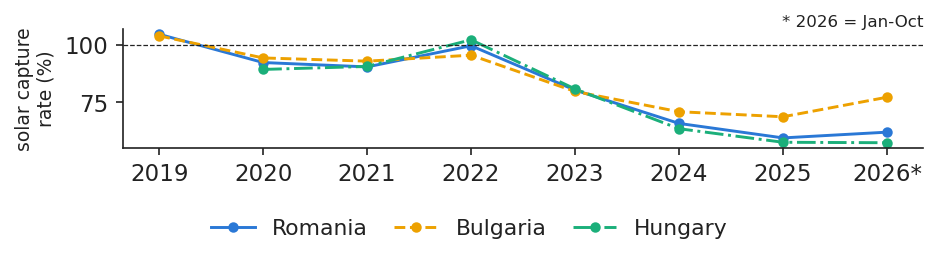
        The chart compares the yearly solar capture rates of the three coupled markets. They fell together: in 2025 the rate was 59.4% in Romania, 68.6% in Bulgaria and 57.5% in Hungary. Coupled markets share their midday surplus, so a park in one country is affected by the parks built in the others.

        In 2026 the Bulgarian rate rose to 77.1%, at the same time as the Bulgarian battery fleet grew. This is an association, not a proof, but the mechanism is plausible: batteries that charge at midday add demand exactly when solar produces and lift the midday price.

        In practice: batteries charging at midday raise the price solar sells at: solar gains from other people's batteries.
        Chart: Regional cannibalisation: Romanian, Bulgarian and Hungarian capture rates fell in step

        Yearly solar capture rates in Romania, Bulgaria and Hungary, 2019 (Hungary 2020) to Oct 2026.

        Source: energy-charts.info (Fraunhofer ISE); day-ahead prices (OPCOM, IBEX, HUPX); ENTSO-E solar output and load. Data: 2019 (Hungary 2020) to 2026-10-31; Bulgaria: hourly solar output.

        In 2025, 32.1% of Romanian solar output was sold in the cheapest 10% of hours

        Slide 18 in the PDF

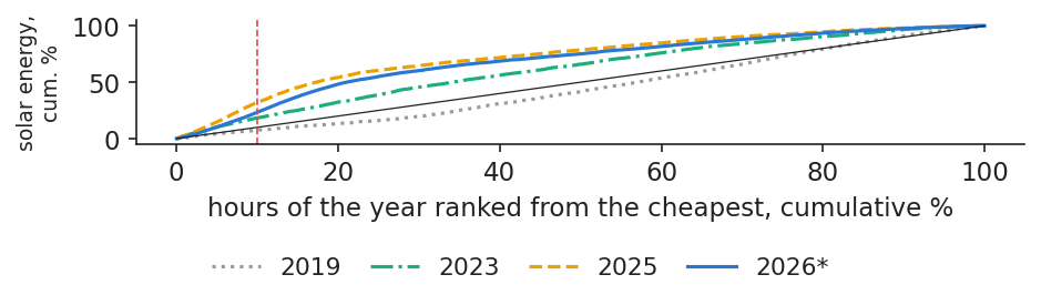
        Another way to see cannibalisation is to rank the hours of each year from the cheapest to the dearest and ask how much of the year's solar energy was produced up to each rank. The chart draws this curve for every year. If solar were spread evenly over the year, the cheapest 10% of hours would carry 10% of its output.

        In 2019 the cheapest 10% of hours carried only 7.6% of Romanian solar output. In 2025 they carried 32.1%, and in 2026 23.4%. In 2025, 9.6% of solar output was produced at zero or negative prices. A large and growing part of solar energy is sold precisely when electricity is worth least.

        In practice: as announced in Lecture 1: a solar park without storage sells much of its output in the cheapest hours of the year.
        Chart: In 2025, 32.1% of Romanian solar output was sold in the cheapest 10% of hours

        Cumulative share of the year's Romanian solar output against the rank of the hour, hours ranked from the cheapest, one curve per year.

        Source: energy-charts.info (Fraunhofer ISE); OPCOM prices; ENTSO-E solar, wind and load (Transelectrica data for Romania). Data: each calendar year; 2026 to 2026-10-31.

        Section summary

        The capture rate of Romanian solar fell from 104.5% in 2019 to 59.4% in 2025, while wind stayed close to 100%. The fall is regional and tied to the growth of solar output: the more solar, the lower its own price.

        Negative prices

        Since 2023, the Romanian day-ahead price sometimes falls below zero. This section explains why a producer would offer to pay for producing, counts negative prices correctly, values switching a park off, and shows what the 15-minute market reveals that hourly averages hide.

        A producer bids below zero when stopping costs more than paying to produce

        Slide 20 in the PDF

        A plant offers at the cost of one more MWh minus what it earns or saves only by running:

        \[b_i=c_i-s_i-k_i\]
        (6.7)

        where \(b_i\) is the offer of plant \(i\) in EUR/MWh, \(c_i\) its marginal cost, \(s_i\) the support paid per MWh produced, and \(k_i\) the cost of a stop and restart expressed per MWh. When \(s_i+k_i\) exceeds \(c_i\), the offer is negative. Two groups bid below zero: plants whose output is paid per MWh by a support scheme or a contract, and plants such as nuclear and run-of-river hydro, which cannot stop cheaply (Fanone, Gamba & Prokopczuk, 2013).

        Negative prices are counted in hour-equivalents:

        \[h^{-}=\sum_t \Delta_t\,\mathbf 1[P_t<0]\]
        (6.8)

        where \(\Delta_t\) is the length of interval \(t\) in hours and \(\mathbf 1[P_t<0]\) equals one when the price of the interval is negative. In 2025 Romania had 196 negative hours, with a mean negative price of −10.5 EUR/MWh; the lowest price of 2026 was −99.75 EUR/MWh.

        In practice: a merchant solar park has \(b_i\approx 0\): it should stop as soon as the price turns negative.

        Romania had 196 negative hours in 2025, Germany 575

        Slide 21 in the PDF

        The chart counts negative hours per year with (6.8) in Romania, Bulgaria, Hungary and Germany. Germany, with far more solar and wind, has many more: 575 hours in 2025. Romania had 196.

        Comparing the same months, Jan–Oct, the count fell in 2026: in Romania from 196 to 171.75 hours, in Hungary from 281 to 223.5 hours. This happened even though solar output grew. Possible reasons are a higher general price level and more batteries charging at midday, which add demand precisely in the hours that used to turn negative. The counting rule is that of Lecture 1: a 15-minute interval counts 0.25 h.

        In practice: a supplier with flexible industrial clients can be paid to consume in these hours.

        Interactive chartInteractive page →

          Code of this chart: EMQA_L6_neg_hours · open in Colab

          Negative hours per year in Romania, Bulgaria, Hungary and Germany–Luxembourg, 2022 to Oct 2026, in hour-equivalents.

          Source: energy-charts.info (Fraunhofer ISE); day-ahead prices of OPCOM (RO), IBEX (BG), HUPX (HU), EPEX SPOT (DE-LU), via ENTSO-E. Data: 2022 to 2026-10-31; a 15-min interval counts 0.25 h.

          Question for the room In Romania, in which months and hours are the negative prices of 2026 concentrated, and how deep are they?
          Answer

          In the middle of the day (roughly 10:00–16:00) of the spring months, when solar output is high, demand moderate and hydro plants run. The heat map counts hour-equivalents (a 15-minute interval counts 0.25 h); the right panel shows the duration-weighted mean of the negative prices by month. Choose 2022: Romania had no negative price before May 2023.

          Revenue losses: low positive midday prices cost more than negative prices

          Slide 22 in the PDF

          A merchant park, without support per MWh, gains \(|P_t|\) for each MWh it does not produce at a negative price. Its gain from stopping in every negative interval, per MWh of yearly output, is

          \[g=\frac{\sum_t \max(0,-P_t)\,G_t\Delta_t}{\sum_t G_t\Delta_t}\]
          (6.9)

          where \(G_t\) is solar output in MW, \(\Delta_t\) the interval length, and \(\max(0,-P_t)\) the amount paid per MWh when the price is negative. The relevant comparison is with the profile discount \(B-\mathrm{CP}\) of the previous section.

          In 2025, 6.2% of Romanian solar output was produced at negative prices, which cost the parks 1.71 million EUR. Yet the gain from switching off was only \(g\) = 0.63 EUR/MWh, against a profile discount of 43.9 EUR/MWh. In 2026, 4.0% of output was produced at negative prices and \(g\) = 0.35 EUR/MWh. Negative prices attract attention, but the large loss of a solar park comes from the many midday hours with low positive prices.

          In practice: install remote switch-off because it is cheap, but value a park on its capture price.

          Quarter-hours reveal 26 negative prices hidden inside hours with a non-negative average

          Slide 23 in the PDF

          Since 1 Oct 2025, the Single Day-Ahead Coupling (SDAC) of European markets uses a 15-minute MTU (NEMO Committee, 2025). From that date to 31 Oct 2026, Romania had 687 negative quarter-hours, equal to 171.75 hour-equivalents. Of these, 26 (3.8%) fall in hours whose average price is zero or positive.

          This matters because hourly averages show only 195 negative hours. A battery or a flexible load that acts per quarter-hour can use the hidden negative quarter-hours; a park metered per quarter-hour pays them. The counting rule is (6.8) with \(\Delta_t\) = 0.25 h: a quarter-hour must never be counted as an hour.

          In practice: set switch-off and battery logic on the 15-minute grid, as the market now is.

          Section summary

          Producers bid below zero when support or restart costs make stopping expensive. Romanian negative hours are fewer than in Germany and fell in 2026; switching off saves little compared with the low positive midday prices.

          Intraday shape and price spreads

          Low midday prices and high evening prices create a daily price shape. This section reads that shape on 15-minute prices, defines the daily spread that a battery earns, and compares it across Romania and its neighbours.

          Spring quarter-hour prices: 23.0 at midday, 208.3 EUR/MWh in the evening

          Slide 25 in the PDF

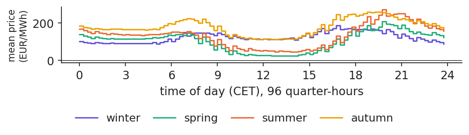
          The chart shows the mean price of each quarter-hour of the day in the last 12 months, separately for each season. In spring the profile forms a deep "solar valley": the minimum, 23.0 EUR/MWh, falls at 12:45 CET and the maximum, 208.3 EUR/MWh, at 19:45 CET, when the sun has set and demand is still high.

          The distance between the maximum and the minimum measures the daily opportunity for storage. It is 185 EUR/MWh in spring and 226 in summer, but only 98 EUR/MWh in winter, when solar output is small and the valley almost disappears.

          In practice: a battery charges in the valley and discharges on the evening ramp; the gap is its gross margin.
          Chart: Spring quarter-hour prices: 23.0 at midday, 208.3 EUR/MWh in the evening

          Mean 15-minute price profile of the Romanian day-ahead market by season, last 12 months (Nov 2025 – Oct 2026), CET.

          Source: energy-charts.info (Fraunhofer ISE); OPCOM day-ahead prices for Romania, via ENTSO-E. Data: last 12 months 2025-11-01 to 2026-10-31, 15-min prices, CET; winter = Dec-Feb, spring = Mar-May, summer = Jun-Aug, autumn = Sep-Nov.

          A battery earns the spread between dear and cheap hours, minus its losses

          Slide 26 in the PDF

          A battery buys a MWh when it is cheap and sells what survives the round trip when it is dear. A first measure of its business case is the daily spread between the \(k\) dearest and the \(k\) cheapest hours, and the approximate gross margin of one cycle:

          \[S^{(k)}_d=\bar P^{\,\mathrm{top}\,k}_d-\bar P^{\,\mathrm{bot}\,k}_d\]
          (6.10)
          \[\pi_d\approx k\,\big(\eta\,\bar P^{\,\mathrm{top}\,k}_d-\bar P^{\,\mathrm{bot}\,k}_d\big)\]
          (6.11)

          where \(\bar P^{\,\mathrm{top}\,k}_d\) and \(\bar P^{\,\mathrm{bot}\,k}_d\) are the mean prices of the \(k\) dearest and the \(k\) cheapest hours of day \(d\), \(k\) is the number of hours of storage, \(\eta\) the round-trip efficiency (85%), and \(\pi_d\) the gross margin of one cycle of a 1 MW battery, in EUR.

          For Romania and \(k=2\), the mean daily spread was 45 EUR/MWh in 2019, 151 in 2025 and 174 in 2026. Losses set a threshold: a battery that buys at 50 EUR/MWh must sell above \(50/0.85\approx59\) EUR/MWh to break even, because only 85% of the energy comes back (Sioshansi et al., 2009).

          In practice: a battery developer reads the business case from the daily spread, before any model.

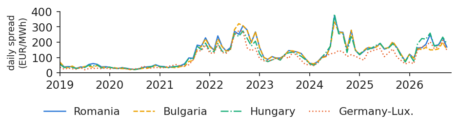
          The daily spread is about four times its 2019 level and similar in Romania, Bulgaria and Hungary

          Slide 27 in the PDF

          The chart follows the monthly mean of the daily 2-hour spread (6.10) in the four markets since 2019. The spread rose with the energy crisis of 2022, did not return to its old level afterwards, and is now about four times its 2019 level. In 2026 the mean spread between the dearest 2 and the cheapest 2 hours was 174 EUR/MWh in Romania, 150 in Bulgaria, 187 in Hungary and 152 in Germany.

          The three neighbouring markets have very similar spreads because they are coupled: every battery in the region competes for the same spread, and a battery built in Bulgaria lowers it in Romania too.

          In practice: treat the spread as a regional resource, shared with every new battery next door.
          Chart: The daily spread is about four times its 2019 level and similar in Romania, Bulgaria and Hungary

          Monthly mean of the daily spread between the 2 dearest and the 2 cheapest hours, Romania, Bulgaria, Hungary and Germany–Luxembourg, 2019 to Oct 2026.

          Source: energy-charts.info (Fraunhofer ISE); day-ahead prices of OPCOM (RO), IBEX (BG), HUPX (HU), EPEX SPOT (DE-LU), via ENTSO-E. Data: daily, hourly prices (15-min averaged), monthly means, 2019 to 2026-10-31.

          Section summary

          The solar valley creates a large daily spread, widest in spring and summer. The 2-hour spread is about four times its 2019 level and is shared across the coupled region.

          The economics of a battery

          The daily spread is only a first measure. This section computes the revenue of a battery with an optimal daily schedule, compares perfect foresight with simple forecast rules and hourly with 15-minute prices, shows how batteries erode their own spread, and turns the revenue into a maximum investment.

          The best daily schedule of a battery solves a small linear programme

          Slide 29 in the PDF

          The battery chooses when to charge and discharge to maximise revenue, within its physical limits. For each day it solves

          \[\max_{c,\,x}\ \sum_t P_t\,(x_t-c_t)\,\Delta_t\]
          (6.12)
          \[e_t=e_{t-1}+\big(\sqrt\eta\,c_t-x_t/\sqrt\eta\big)\Delta_t\]
          (6.13)
          \[0\le e_t\le E,\quad e_0=e_T=0,\quad 0\le c_t,x_t\le 1,\quad \sum_t x_t\Delta_t\le\sqrt\eta E\]
          (6.14)

          where \(c_t\) and \(x_t\) are the charging and discharging power in MW, \(P_t\) the price and \(\Delta_t\) the interval length, \(e_t\) the stored energy in MWh, \(E\) the storage capacity (1, 2 or 4 MWh for a 1 MW battery), \(\eta\) = 0.85 the round-trip efficiency, split equally between charging and discharging, and \(T\) the number of intervals of the day. The last constraint allows at most one cycle a day (Appendix B gives the matrix form).

          The assumptions, 85% round trip and one cycle a day, are the reference values of the National Renewable Energy Laboratory (NREL) of the United States (Cole & Karmakar, 2023). Capacity fade, fees and balancing revenue are not included. The programme is solved under two information sets: with perfect foresight, when prices are known in advance, which gives an upper bound, and with a forecast rule, when the schedule is optimised on a forecast but paid at the real prices.

          In practice: this programme, with your own prices and limits, is the core of every battery dispatch tool.

          With perfect foresight, a 2-hour battery earned 111.2 thousand EUR per MW in the last 12 months

          Slide 30 in the PDF

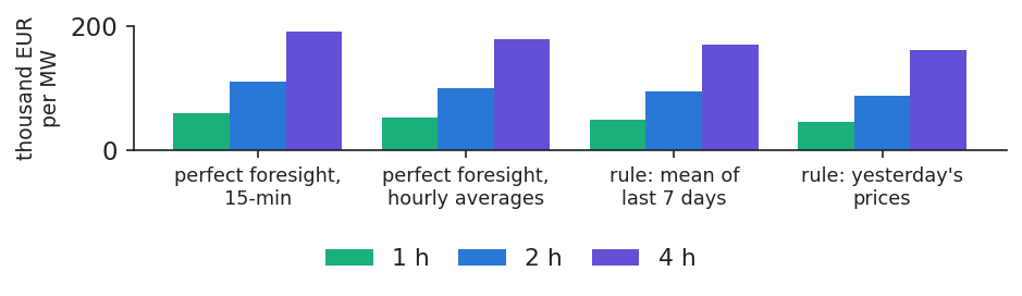
          The chart shows the yearly revenue of 1-, 2- and 4-hour batteries of 1 MW, from (6.12) with perfect foresight. For 2 hours, revenue was 26.3 thousand EUR per MW-year in 2019, 125.0 in 2022 and 98.7 in 2025; in the last 12 months it reached 111.2 thousand EUR.

          Longer batteries earn more, but not proportionally. A 4-hour battery earns 1.72 times what a 2-hour battery earns, not twice as much, because its third and fourth hours trade a smaller spread: the cheapest and dearest hours of the day are already used by the first two.

          In practice: size the battery on the revenue of each extra MWh of storage, not on total revenue.

          Interactive chartInteractive page →

            Code of this chart: EMQA_L6_bat_years · open in Colab

            Yearly arbitrage revenue of 1-, 2- and 4-hour batteries with perfect foresight, thousand EUR per MW, 2019–2025 and the last 12 months.

            Source: energy-charts.info; day-ahead prices via ENTSO-E; ENTSO-E battery output (BG, RO); own optimisation. Data: 1 MW, round trip 85%, max one cycle a day; 2019-2025 and last 12 months 2025-11-01 to 2026-10-31.

            Question for the room A 1-MW battery with 2 hours of storage and 85% round-trip efficiency earned about 98.7 thousand EUR in Romania in 2025 with perfect foresight. Does a 4-hour battery earn twice as much?
            Answer

            No: 165.2 thousand EUR, i.e. 1.67 times as much. The extra hours of storage buy energy in less cheap hours and sell it in less expensive ones, so each MWh of capacity earns less (and the real schedule is decided on forecasts, not on known prices: with the mean profile of the previous week the lecture keeps about 85% of the perfect-foresight revenue). Move the efficiency: from 75% to 95%, the revenue of the 2-hour battery in Romania rises by 39–46% in 2019–2022 but only by 21–22% in 2024–2026, when the deep midday troughs (down to negative prices) make the buying price small compared with the selling price, so the losses cost less.

            A simple 7-day rule earns 85% of the 2-hour perfect-foresight revenue

            Slide 31 in the PDF

            A real battery does not know tomorrow's prices. The lecture tests two rules that use only information available at 12:00 CET on the day before delivery, \(d-1\), when bids are due. The first uses the mean price profile of the last 7 days; the second uses yesterday's prices. The schedule is optimised on the forecast and paid at real prices.

            The 7-day rule earns 82%, 85% and 89% of the perfect-foresight revenue for 1-, 2- and 4-hour batteries. Yesterday's prices earn 75%, 79% and 84%. Longer batteries forgive timing errors better: if the cheapest hour is missed by one hour, a 4-hour battery still charges in cheap hours. The comparison is made on 361 common days and scaled to the full period.

            In practice: budget on a rule you can actually run; a better forecast (Lecture 2) closes part of the gap.
            Chart: A simple 7-day rule earns 85% of the 2-hour perfect-foresight revenue

            Revenue in thousand EUR per MW of 1-, 2- and 4-hour batteries in the last 12 months: perfect foresight on 15-minute prices and on hourly averages, the 7-day rule and yesterday's prices.

            Source: energy-charts.info; day-ahead prices via ENTSO-E; ENTSO-E battery output (BG, RO); own optimisation. Data: last 12 months 2025-11-01 to 2026-10-31; 1 MW, round trip 85%; forecast rules on 361 common days, scaled to the full period.

            Forecasting the whole price distribution helps a battery bid

            Slide 32 in the PDF

            The rules above use a single forecast price per hour. A study of our group (Andrei, Cepoi, Dumitrescu, Lessmann, Luchian, Pele & Petukhina, 2026, doi:10.2139/ssrn.6872381), presented by Cosmin Octavian Cepoi at the AIDA 2026 conference (slides), forecasts instead the whole joint distribution of the next day's 96 hourly prices: 24 hours in Romania, Bulgaria, Hungary and Czechia. It uses a distributional random forest with 37 predictors on data from January 2018 to September 2024, re-estimated on 70 rolling windows (365 days to train, the next 30 days to test). The median of the forecast picks the charge hour and the later discharge hour; quantiles of the forecast set the buy and sell limit prices.

            Forecast errors are highest at 17:00–18:00, usually the discharge hours, which is where a single point forecast is weakest. For a 1 MW / 1 MWh battery in Romania, the cumulative profit is 143.0 thousand EUR with the quantile rule, against 133.2 with fixed hours and 188.2 with perfect foresight; the quantile rule beats the fixed-hour rule in all four markets, and trading across markets adds value (150.3 thousand EUR). With an upfront investment of 500,000 EUR, 90% efficiency, 15 years and a 7% discount rate, day-ahead arbitrage alone does not cover the investment, the same message as the break-even investment computed later in this section.

            In practice: bid from forecast quantiles, not from a single price forecast: the hours that pay are in the tails.

            15-minute prices raised a 1-hour battery's revenue by 14.5% on the same days

            Slide 33 in the PDF

            Any hourly schedule can also be run on quarter-hours, so finer prices can only add revenue:

            \[R^{15}=\max_{c,x}\sum_t P^{15}_t(x_t-c_t)\tfrac14\ \ge\ R^{60}\]
            (6.15)

            where \(R^{15}\) is the optimal revenue on the 96 quarter-hour prices \(P^{15}_t\) of a day, \(R^{60}\) the optimal revenue when each hour is paid the mean of its four quarters, and \(c_t\), \(x_t\) the charging and discharging power. Both are computed on the same days, so the difference is the value of granularity alone.

            In the last 12 months, in thousand EUR per MW, the 1-hour battery earned 53.2 on hourly prices and 61.0 on 15-minute prices (+14.5%), the 2-hour battery 100.8 and 111.2 (+10.3%), and the 4-hour battery 178.4 and 190.9 (+7.0%). A comparison with the hourly year before would mix in changes in the price level, which is why both revenues use the same days.

            In practice: short batteries gain most from 15-minute prices.

            Batteries cannibalise their own spread: on the local order book, 50 MW would have closed it on 21 Oct 2026

            Slide 34 in the PDF

            Batteries are subject to the same cannibalisation as solar. Charging adds demand at midday and discharging adds supply in the evening, so both pull the two prices together. On the OPCOM curves the effect can be computed as

            \[\Delta P(X)=p^{*}_{\text{eve}}(+X\text{ supply})-p^{*}_{\text{mid}}(+X\text{ demand})\]
            (6.16)

            where \(X\) is the battery power in MW and \(p^*\) the clearing price recomputed on the OPCOM curves of 12:00–12:15 and 20:00–20:15 (Romanian time), with \(X\) added as demand at midday and as supply in the evening; cross-border flows are held fixed (Appendix C).

            On 21 Oct 2026, the actual evening price exceeded the midday price by 91.77 EUR/MWh. With 50 MW of batteries the difference would have been −13.15 EUR/MWh, and with 100 MW −47.12: on the local order book alone, 50 MW are enough to close the spread. Like the merit-order computation, this is an upper bound, because in the coupled market flows adjust. Fleets are already running: Romanian batteries delivered up to 766 MW in 2026, and Bulgarian ones, reported since 9 Sep 2026, up to 2,795 MW.

            In practice: model the spread after the fleet is built, not the spread seen before it.

            A Romanian battery competes for the same regional spread as the Bulgarian and Hungarian ones

            Slide 35 in the PDF

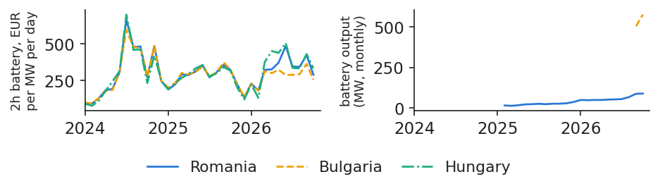
            The chart follows the monthly perfect-foresight revenue of a 2-hour battery in Romania, Bulgaria and Hungary since 2024. In the last 12 months, in thousand EUR per MW, it was 117.6 in Hungary, 111.2 in Romania, 96.4 in Bulgaria and 90.6 in Germany. The right panel shows the output of the battery fleets reported to ENTSO-E in Romania and Bulgaria.

            Daily revenues move together: their correlation with Romania is 0.80 for Bulgaria and 0.87 for Hungary. A good day for a Romanian battery is a good day for the batteries of the neighbours, and each of them takes part of the same evening spread.

            In practice: as announced in Lecture 1: a Romanian battery developer competes for the same regional evening spread.
            Chart: A Romanian battery competes for the same regional spread as the Bulgarian and Hungarian ones

            Left: revenue of a 2-hour battery with perfect foresight, EUR per MW per day, monthly, in Romania, Bulgaria and Hungary; right: monthly battery output reported to ENTSO-E in Romania and Bulgaria; Jan 2024 to Oct 2026.

            Source: energy-charts.info; day-ahead prices via ENTSO-E; ENTSO-E battery output (BG, RO); own optimisation. Data: 2h battery, perfect foresight, 2024-01 to 2026-10; battery output as reported to ENTSO-E.

            At 8% over 15 years, the 2-hour revenue supports at most 808 EUR per kW

            Slide 36 in the PDF

            The largest investment that a yearly revenue can repay is that revenue multiplied by the annuity factor:

            \[I^{\max}=R\cdot a(r,n)\]
            (6.17)
            \[a(r,n)=\sum_{j=1}^{n}(1+r)^{-j}=\frac{1-(1+r)^{-n}}{r}\]
            (6.18)

            where \(R\) is the yearly revenue per MW in EUR, \(r\) the discount rate (8%, an assumption), \(n\) the lifetime (15 years, from NREL) and \(a(r,n)\) the annuity factor, here 8.56 (Appendix D). Dividing \(I^{\max}\) by 1,000 gives EUR per kilowatt (kW).

            For a 2-hour battery in the last 12 months, perfect foresight supports at most 952 EUR/kW, and the 7-day rule 808 EUR/kW, which is 404 EUR per kilowatt-hour (kWh) of storage. Several items are not included: operating costs, grid tariffs and capacity fade would lower \(I^{\max}\); balancing revenue would raise it; and new fleets shrink the spread (Schmidt et al., 2019).

            In practice: compare 404 EUR/kWh with the turnkey quote before anything else.

            Section summary

            A 2-hour battery earned 111.2 thousand EUR per MW in the last 12 months with perfect foresight, and about 85% of that with a simple rule. 15-minute prices add revenue, new batteries erode the spread, and at 8% over 15 years the revenue supports at most 808 EUR per kW.

            Case studies: Apr 2026 and summer 2026

            Two case studies apply the tools of the lecture to real episodes: April 2026, the month with the most negative hours, and summer 2026, when Romania exported at midday and imported from Bulgaria in the evening.

            Case study: in the week of 20 Apr 2026, Romania had 24 negative hours and solar captured 42%

            Slide 38 in the PDF

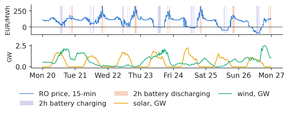
            The chart shows the 15-minute prices and the solar and wind output of Romania in the week from 20 to 26 Apr 2026, with the intervals in which a 2-hour battery with perfect foresight charges and discharges. The week had 24 negative hours. Prices ranged from −99.75 EUR/MWh, on 26 Apr at 13:00, to 328.00 EUR/MWh; solar output peaked at 2,243 MW.

            For solar the week was poor: its capture price was 37.0 EUR/MWh against a baseload price of 87.0, a capture rate of 42.5%. For a battery the same week was among the best: a 2-hour battery with perfect foresight earned 391 EUR per MW a day, against 305 on an average day of the last 12 months.

            In practice: the same sunny week is the worst for a solar park and among the best for a battery.
            Chart: Case study: in the week of 20 Apr 2026, Romania had 24 negative hours and solar captured 42%

            Romanian 15-minute day-ahead price with the charging and discharging intervals of a 2-hour battery (top) and solar and wind output in GW (bottom), 20–26 Apr 2026, CET.

            Source: energy-charts.info (Fraunhofer ISE); OPCOM prices; ENTSO-E solar, wind and load (Transelectrica data for Romania). Data: week 2026-04-20 to 2026-04-26, 15-min, CET.

            Case study: implications of Apr 2026 for each participant in the Romanian market

            Slide 39 in the PDF

            April 2026 had 67 negative hours, the most of any month. The same month meant different things to different players:

            • Solar developer: capture rate 49.4% (47.2 against 95.6 EUR/MWh), with 17.9% of output at negative prices. The decision is between storage on site and a PPA that prices the solar profile.
            • Wind developer: capture rate 97.8%. In Romania, wind is not the cannibalised technology.
            • Battery developer: a 2-hour battery earned 325 EUR per MW a day, against 305 on average over the last 12 months.
            • Supplier and industrial consumer: 67 negative hours. Moving consumption to spring middays is paid.
            • Transelectrica: after sunset, the evening ramp and the interconnectors set the price.

            Case study: midday exports and evening imports from Bulgaria, summer 2026

            Slide 40 in the PDF

            The chart shows the mean hourly cross-border flows of Romania and the prices of Romania and Bulgaria between 1 Jun and 31 Aug 2026; positive flows are imports into Romania. At midday Romania exports: 960 MW net at 12:00 across all borders, mostly to Hungary (857 MW) and Serbia (367 MW). It exported to Bulgaria between 12:00 and 15:00 on only 43 of the 92 days.

            In the evening the direction reverses: Romania imports from Bulgaria, 2,064 MW at 21:00, on all 92 days. At 21:00 the mean price was 243.9 EUR/MWh in Romania and 178.3 in Bulgaria. When the border is fully used, the two prices separate, and the Romanian evening price stays higher. The borders with Moldova and Ukraine are only partly reported.

            In practice: the evening gap of 65.6 EUR/MWh is what evening storage and more interconnection capacity are worth in Romania.

            Interactive chartInteractive page →

            Borders

              Code of this chart: EMQA_L6_rogb_summer · open in Colab

              Mean flow by hour of the day, Romania's net flow on all borders and the flow on the Romania–Bulgaria border (+ = import into Romania), and day-ahead prices of Romania and Bulgaria, 1 Jun – 31 Aug 2026.

              Source: energy-charts.info (Fraunhofer ISE): cross-border physical flows of Romania (ENTSO-E); day-ahead prices of OPCOM (RO) and IBEX (BG). Data: hourly means, 2026-06-01 to 2026-08-31; Moldova and Ukraine borders only partly reported.

              Question for the room In summer 2026 (1 June–31 August), Romania exported at midday and imported in the evening. From which neighbour did the evening imports come, and why?
              Answer

              From Bulgaria, on all 92 days: at 21:00 Romanian time, the mean flow on the Romania–Bulgaria border was 2,064 MW towards Romania. At that hour the mean Romanian price was 243.9 EUR/MWh and the Bulgarian one 178.3 EUR/MWh (gap 65.6 EUR/MWh): the interconnector was congested, otherwise market coupling would have equalised the two prices. At midday both prices were about 50 EUR/MWh and Romania exported, mostly to Hungary (857 MW) and Serbia (367 MW).

              Section summary

              In a sunny spring week, the same prices that cut the capture rate of solar to 42.5% lift the daily margin of a battery well above its average. In summer, the full Bulgarian border in the evening keeps the Romanian price above the Bulgarian one.

              Wrap-up

              The wrap-up checks the main ideas with four questions, summarises the lecture, presents related research from our group and lists resources for further study.

              Self-assessment questions

              Slide 41 in the PDF
              1. A solar PPA is offered at the 2025 baseload forward of 108 EUR/MWh. What does the solar profile really earn?
                Answer: about 64 EUR/MWh in 2025, because the capture rate was 59%. A buyer who pays the baseload price for the solar profile pays a large premium.
              2. Since 1 October 2025, Romania has had 687 negative quarter-hours. How many negative hours do you report?
                Answer: 171.75 hour-equivalents, since each quarter-hour counts 0.25 h, not 687 hours.
              3. Doubling storage from 2 h to 4 h doubles the cost of the cells. Does it double revenue?
                Answer: no. In the last 12 months a 4-hour battery earned 1.72 times what a 2-hour one earned, because the extra hours trade a smaller spread.
              4. On the OPCOM curves of 21 Oct 2026, 25 MW more at zero price lower the midday price to 131.4 EUR/MWh. Is this what a new 25 MW park does?
                Answer: no. The curves hold cross-border flows fixed; in the coupled market part of the extra output is exported, so the true effect is smaller. The regression gives a fall of about 27 EUR/MWh per GW.

              Solar lowers the price it is paid: the Romanian solar capture rate fell from 104% in 2019 to 59% in 2025, while wind stayed near 100%. Batteries live on the same regional spread that solar creates: a 2-hour battery earned 111 thousand EUR per MW in the last 12 months with perfect foresight, and about 85% of that with a simple forecast rule. Lecture 7 continues the course.

              Research from our group on renewables and Romanian prices

              Slide 46 in the PDF

              Several papers from our group study the Romanian market with the same drivers as this lecture. The findings below are as stated in the papers; the numbers on the other parts of this page come from our own data.

              • Explaining price drops and spikes (Andrei & Pele, 2025): the paper detects unusual hourly Romanian prices with an isolation forest and explains them with Shapley values. Wind and solar output drive the price drops; load forecast errors and conventional generation drive the spikes.
              • Price drivers by horizon and regime (Andrei, Pele & Cramer, 2026): the paper forecasts Romanian hourly prices for 2018–2024 with tree ensembles and measures which drivers matter at each horizon and in low-, normal- and high-price regimes. It identifies the renewable drivers behind the low-price regime studied in this lecture.
              • Early warning of spikes (Andrei, Pele, Cramer, Amza & Diaconu, 2026): the paper builds an explainable artificial intelligence (AI) early-warning system for Romanian price spikes. The residual-load forecast is the main driver, the same variable as in our regression.
              • Price elasticity of demand (Proșcanu, Proșcanu & Pele, 2025): the paper tests Granger causality between Romanian consumption and price. Consumption does not react to price, which explains the almost vertical demand curve of the merit order.

              Further reading and resources

              Slide 47 in the PDF
              • Hirth (2013): the reference paper on the value factor of wind and solar, doi:10.1016/j.eneco.2013.02.004.
              • Cole & Karmakar (2023): battery costs, efficiency and lifetime used in this lecture, doi:10.2172/1984976.
              • energy-charts.info: live prices, generation and installed capacity for Romania and its neighbours, energy-charts.info.
              • This course: code, data and notebooks, github.com/danpele/EMQA.
              • OPCOM aggregated curves: download another day and repeat the merit-order computation, opcom.ro.
              • Experiment yourself: the notebook reproduces every chart and number of this lecture.

              Appendix

              The appendix gives the derivations and computational details behind the capture rate, the battery programme, the recomputation of the clearing price and the annuity factor.

              Appendix A: the capture rate is one plus a scaled covariance

              Slide 51 in the PDF

              Define the duration weights and the weighted means and covariance:

              \[w_t=\frac{\Delta_t}{\sum_s\Delta_s},\quad \bar P=\sum_t w_tP_t=B,\quad \bar G=\sum_t w_tG_t,\quad \mathrm{Cov}_\Delta(P,G)=\sum_t w_t(P_t-\bar P)(G_t-\bar G)\]

              where \(w_t\) is the weight of interval \(t\), proportional to its length \(\Delta_t\), and \(P_t\), \(G_t\) are price and output. Dividing the numerator and the denominator of CP in (6.4) by \(\sum_s\Delta_s\) gives \(\mathrm{CP}=\sum_t w_tP_tG_t/\bar G\). By the definition of the covariance, \(\sum_t w_tP_tG_t=\mathrm{Cov}_\Delta(P,G)+\bar P\bar G\). Therefore

              \[\mathrm{CR}=\frac{\mathrm{CP}}{\bar P}=1+\frac{\mathrm{Cov}_\Delta(P,G)}{\bar P\,\bar G}\]

              For Romanian solar in Jan–Oct 2026, \(\bar P\) = 137.4, \(\bar G\) = 593 MW and the covariance is −31,069, so CR = 0.619. CR is below one exactly when output is high in cheap intervals, and it is undefined if \(\bar P\le 0\) (Hirth, 2013).

              Appendix B: the battery programme in matrix form

              Slide 52 in the PDF

              The variables are stacked in one vector \(z=(c_1,\dots,c_T,\,x_1,\dots,x_T,\,e_1,\dots,e_T)\) of \(3T\) variables, where \(T\) is 92, 96 or 100 quarter-hours depending on clock changes (24 hours before October 2025). The objective is to minimise the negative of revenue:

              \[\min_z\ \sum_t P_t\Delta_t c_t-\sum_t P_t\Delta_t x_t\]

              subject to the equalities

              \[e_t-e_{t-1}-\sqrt\eta\,\Delta_tc_t+\Delta_tx_t/\sqrt\eta=0,\quad t=1,\dots,T,\quad e_0=0,\quad e_T=0\]

              and the inequality and bounds \(\sum_t\Delta_tx_t/\sqrt\eta\le E\), \(0\le c_t,x_t\le1\) and \(0\le e_t\le E\), with the symbols of (6.12) to (6.14). The programme is solved with the HiGHS solver in scipy.

              For the forecast rules, the programme is solved on the forecast \(\hat P_t\) (the mean of the last 7 days, or the prices of day \(d-1\)), and revenue is then computed as \(\sum_tP_t(x_t-c_t)\Delta_t\) with the real prices \(P_t\). Days whose length differs from that of the forecast (clock changes) are dropped: 361 of 365 days are kept (Sioshansi et al., 2009).

              Appendix C: recomputing the clearing price on the OPCOM curves

              Slide 53 in the PDF

              OPCOM publishes, for each quarter-hour, the points of the aggregated supply and demand curves (price, cumulative MW) in XML. Block orders, hourly orders and net cross-border flows are added at the price limits, −600 and +4,000 EUR/MWh, as in OPCOM's own chart.

              \(S(p)\) and \(D(p)\) are obtained by linear interpolation between the published points. The new price is the lowest \(p\) with \(S(p)+X\mathbf 1[p\ge0]-D(p)\ge0\), found by bisection on \([-600,4000]\). For battery charging, \(X\) MW of demand at any price are added to \(D\).

              As a check, with \(X=0\) the curves cross on a flat segment: at midday from 152.16 EUR/MWh upwards, in the evening from 206.49. The official prices, 152.23 and 244.00, lie on these segments, and the official price, not the curve, is used at \(X=0\).

              Appendix D: the annuity factor

              Slide 54 in the PDF

              The present value of a constant yearly revenue \(R\) over \(n\) years at rate \(r\) is a geometric sum:

              \[V=\sum_{j=1}^{n}R(1+r)^{-j}=R\,q\,\frac{1-q^{n}}{1-q},\qquad q=(1+r)^{-1}\]

              Since \(q/(1-q)=1/r\), this simplifies to

              \[V=R\,\frac{1-(1+r)^{-n}}{r}=R\,a(r,n)\]

              which is (6.18). The project pays back if the investment \(I\le V\); with \(r\) = 8% and \(n\) = 15, \(a\) = 8.56. Per kWh of storage, \(I^{\max}/E\) with the 7-day rule is 428, 404 and 365 EUR/kWh for 1-, 2- and 4-hour batteries (Cole & Karmakar, 2023).

              Abbreviations

              AIartificial intelligence
              BGBulgaria (bidding zone)
              CETCentral European Time
              CPcapture price
              CRcapture rate (value factor)
              DE-LUGermany–Luxembourg bidding zone
              ENTSO-EEuropean Network of Transmission System Operators for Electricity
              EPEXEPEX SPOT power exchange
              EUReuro
              GWgigawatt = 1 000 MW
              HACheteroskedasticity- and autocorrelation-consistent (standard errors)
              HUHungary (bidding zone)
              HUPXHungarian Power Exchange
              IBEXIndependent Bulgarian Energy Exchange
              ISEFraunhofer Institute for Solar Energy Systems
              kWkilowatt
              kWhkilowatt-hour
              LPlinear programme
              MTUmarket time unit
              MWmegawatt
              MWhmegawatt-hour
              NRELNational Renewable Energy Laboratory (United States)
              OLSordinary least squares
              OPCOMRomanian electricity and gas market operator
              PPApower purchase agreement
              PZUPiața pentru Ziua Următoare (day-ahead market)
              RORomania (bidding zone)
              SDACSingle Day-Ahead Coupling
              SEstandard error
              TWhterawatt-hour
              XMLExtensible Markup Language (data file format)

              References

              • Andrei, A.-V. & Pele, D. T. (2025). Explainable AI for electricity price anomaly detection: A SHAP-driven approach in Romania's energy market. Preprints. doi:10.20944/preprints202508.0410.v1
              • Andrei, A.-V., Cepoi, C., Dumitrescu, B.-A., Lessmann, S., Luchian, A., Pele, D.-T. & Petukhina, A. (2026). Joint probabilistic forecasting for battery arbitrage in day-ahead power markets. SSRN Working Paper 6872381. doi:10.2139/ssrn.6872381
              • Andrei, A.-V., Pele, D.-T. & Cramer, A.-A. (2026). Multi-horizon explainability in energy price forecasting: Disentangling market dynamics and renewable intermittency in Romania's liberalized electricity market. Proceedings of the International Conference on Business Excellence, 20(1), 104–117. doi:10.2478/picbe-2026-0014
              • Andrei, A.-V., Pele, D.-T., Cramer, A.-A., Amza, A. & Diaconu, D. (2026). Explainable AI-based early warning system for electricity price spikes: Evidence from the Romanian market. Proceedings of the International Conference on Business Excellence, 20(1), 4820–4836. doi:10.2478/picbe-2026-0352
              • Basangova, M., Bolovăneanu, V., Conda, A., Erlwein-Sayer, C., Melzer, A., Pele, D. T., Petukhina, A. & Phan, M. (2026). Day-ahead forecasting for redispatch measures using machine learning models. Talk at the AIDA Conference, Bucharest University of Economic Studies, 3 June 2026. github.com/danpele/EMQA
              • Bradbury, K., Pratson, L. & Patiño-Echeverri, D. (2014). Economic viability of energy storage systems based on price arbitrage potential in real-time U.S. electricity markets. Applied Energy, 114, 512–519. doi:10.1016/j.apenergy.2013.10.010
              • Cludius, J., Hermann, H., Matthes, F. C. & Graichen, V. (2014). The merit order effect of wind and photovoltaic electricity generation in Germany 2008–2016: Estimation and distributional implications. Energy Economics, 44, 302–313. doi:10.1016/j.eneco.2014.04.020
              • Cepoi, C. O. (2026). Uncertainty meets opportunity: Joint probabilistic forecasting for battery arbitrage in CEE day-ahead power markets. Talk at the AIDA Conference, Bucharest University of Economic Studies, 3 June 2026. github.com/danpele/EMQA
              • Cole, W. & Karmakar, A. (2023). Cost projections for utility-scale battery storage: 2023 update. NREL/TP-6A40-85332, National Renewable Energy Laboratory. doi:10.2172/1984976
              • Fanone, E., Gamba, A. & Prokopczuk, M. (2013). The case of negative day-ahead electricity prices. Energy Economics, 35, 22–34. doi:10.1016/j.eneco.2011.12.006
              • Hirth, L. (2013). The market value of variable renewables: The effect of solar wind power variability on their relative price. Energy Economics, 38, 218–236. doi:10.1016/j.eneco.2013.02.004
              • Hirth, L., Ueckerdt, F. & Edenhofer, O. (2016). Why wind is not coal: On the economics of electricity generation. The Energy Journal, 37(3), 1–28. doi:10.5547/01956574.37.3.lhir
              • López Prol, J., Steininger, K. W. & Zilberman, D. (2020). The cannibalization effect of wind and solar in the California wholesale electricity market. Energy Economics, 85, 104552. doi:10.1016/j.eneco.2019.104552
              • NEMO Committee (2025). 15-Minute MTU in SDAC was implemented. Single Day-Ahead Coupling (SDAC) press release, 1 October 2025. nemo-committee.eu
              • Proșcanu, C., Proșcanu, M. & Pele, D. T. (2025). The price elasticity of electricity demand in Romania. Journal of Social and Economic Statistics, 14(2), 131–141. doi:10.2478/jses-2025-0009
              • Schmidt, O., Melchior, S., Hawkes, A. & Staffell, I. (2019). Projecting the future levelized cost of electricity storage technologies. Joule, 3(1), 81–100. doi:10.1016/j.joule.2018.12.008
              • Sensfuß, F., Ragwitz, M. & Genoese, M. (2008). The merit-order effect: A detailed analysis of the price effect of renewable electricity generation on spot market prices in Germany. Energy Policy, 36(8), 3086–3094. doi:10.1016/j.enpol.2008.03.035
              • Sioshansi, R., Denholm, P., Jenkin, T. & Weiss, J. (2009). Estimating the value of electricity storage in PJM: Arbitrage and some welfare effects. Energy Economics, 31(2), 269–277. doi:10.1016/j.eneco.2008.10.005
              • Weron, R. (2014). Electricity price forecasting: A review of the state-of-the-art with a look into the future. International Journal of Forecasting, 30(4), 1030–1081. doi:10.1016/j.ijforecast.2014.08.008
              • Würzburg, K., Labandeira, X. & Linares, P. (2013). Renewable generation and electricity prices: Taking stock and new evidence for Germany and Austria. Energy Economics, 40, S159–S171. doi:10.1016/j.eneco.2013.09.011

              Text written for the web version of the lecture; numbers, charts and sources come from the slides and their Quantlets.