

The slide of the lecture is on the left, the same figure on the right, computed in the browser from the same data. The ▶ button moves the parameter step by step.
From Random Walk to Brownian Motion · Quadratic Variation and Itô Calculus · Geometric Brownian Motion · Mean Reversion: the Ornstein–Uhlenbeck Process · Jumps: the Merton Model · Empirical Comparison of the Models · Case Studies: Rough and Persistent Volatility, Drift Bursts
From Random Walk to Brownian Motion
From Random Walk to Brownian Motion: Donsker's Theorem
Answer
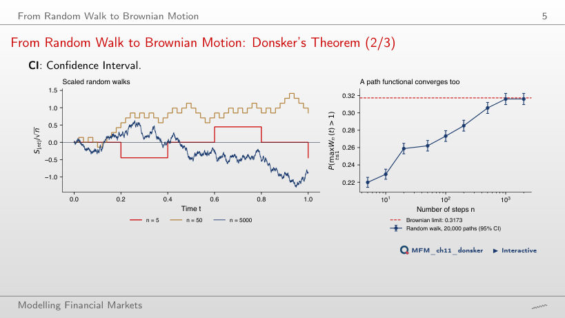
About 0.0455. The reflection principle gives P(max W(t) > 2) = 2[1 − Φ(2)] ≈ 0.0455, against 0.3173 at a = 1. The value 0.0228 = 1 − Φ(2) concerns W(1) alone, not the maximum over the path. The value 0.1587 incorrectly halves the probability at threshold 1: the probability is not inversely proportional to the threshold. On the page, at a = 2, the random walk with n = 2,000 steps gives 0.042. The random-walk curves illustrate convergence to the Brownian benchmark; they do not sample the same Brownian path.
Quadratic Variation and Itô Calculus
Quadratic Variation: Simulation and Data
Answer
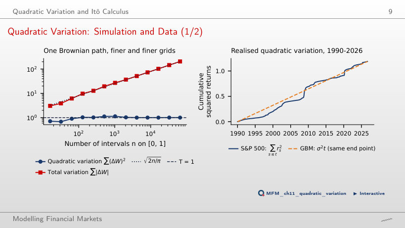
By √2 ≈ 1.41. The mean is n^(1 − p/2)·E|Z|^p, where Z has the standard Normal distribution; for p = 1.5, the factor is 4^0.25 = √2. A factor of 4 ignores the shrinking increments; 1/√2 reverses the direction of the change. This relation concerns the mean, not an exact equality for every path: on the path of the page, the sum goes from 9.75 with 16,384 intervals to 13.83 with 65,536 intervals (ratio 1.42). Only the exponent 2 gives a non-degenerate limit: Σ(ΔW)² tends to T = 1 (1.006 on the finest grid), hence (dW)² = dt.
Geometric Brownian Motion
How Precisely Can We Estimate the Drift?
Answer
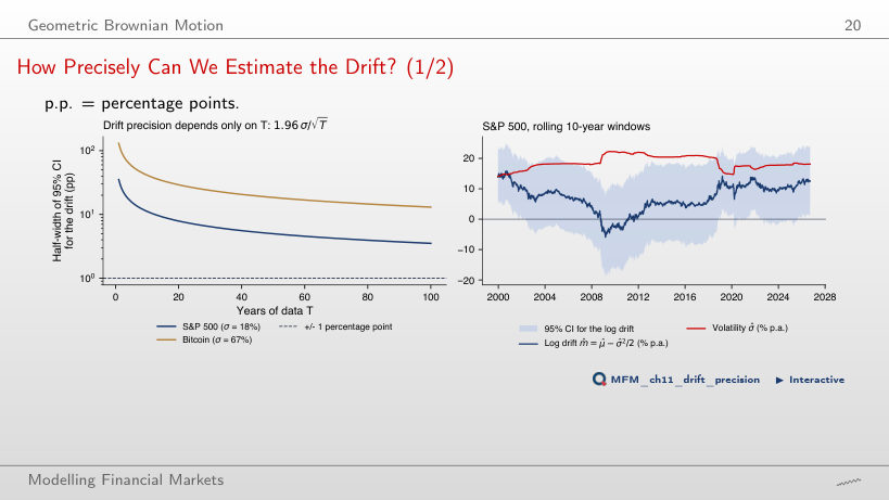
It stays the same. The half-width is 1.96σ/√T: approximately 12.4 percentage points in both cases. Doubling volatility exactly offsets the halving of 1/√T. ‘It halves’ ignores the volatility change; ‘it doubles’ ignores the observation span. For the S&P 500 (σ = 18%), 10 years of data give ±11.2 percentage points, however fine the grid: the 2,520 daily returns do not reduce this half-width. On 10-year windows the log drift ranges from −6.0% (2009-03) to 15.8% (2000-09); with this precision the swings cannot be safely attributed to changes in the drift.
Does GBM Fit the S&P 500?
Answer
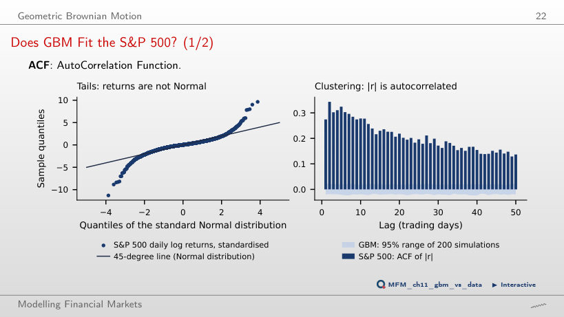
About 0.59 = 9,245 · 2(1 − Φ(4)), counting both tails; one tail would give 0.29. The data have 62, and the worst day lies at −11.3 standard deviations; the excess kurtosis is 10.9. The ACF of |r| is 0.27 at lag 1 and 0.14 at lag 50, while the GBM band stays below 0.024.
Mean Reversion: the Ornstein–Uhlenbeck Process
Vasicek on the 3-Month Treasury Bill Rate
Answer
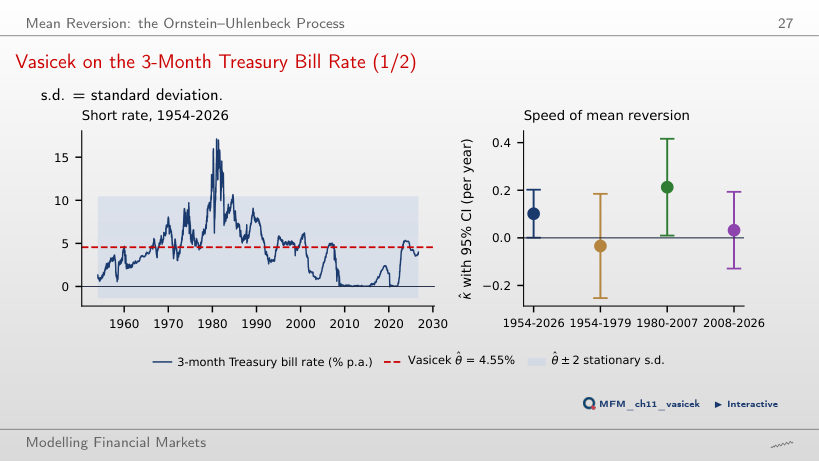
No. κ̂ = 0.101 (SE 0.051) means a half-life of 6.8 years, and the daily AR(1) coefficient is 0.99960, almost a unit root. Over subperiods κ̂ is −0.034, 0.213 and 0.032, and two of the three intervals include zero. The asymptotic interval over 1954–2026 barely excludes zero (0.101 − 1.96 · 0.051 = 0.001), but near a unit root the distribution of κ̂ is not Normal and is biased upwards; the bootstrap test of the random-walk null gives a p-value of 0.287.
Jumps: the Merton Model
Merton Fit to the Return Distribution
Answer
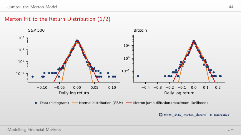
About 33.3%. The daily jump count has a Poisson distribution with mean 102/252 = 0.405; the required probability is 1 − exp(−102/252) ≈ 33.3%. The value 40.5% confuses the expected jump count with the probability of at least one jump; 66.7% is the probability of no jump. A model jump is not automatically a crash: the estimated standard deviation of jump size is 1.44%. The jumps account for 71% of the variance and fit the shape of the marginal distribution; they do not reproduce volatility clustering. The implied excess kurtosis is 3.7 against 10.9 in the data. At λ = 0, preserving the fitted Merton model’s mean and variance, the S&P 500 log-likelihood is 28,291, against 29,500 at the MLE; for a separately refitted GBM, it is 28,300.
Empirical Comparison of the Models
Which Model Reproduces the S&P 500?
Answer
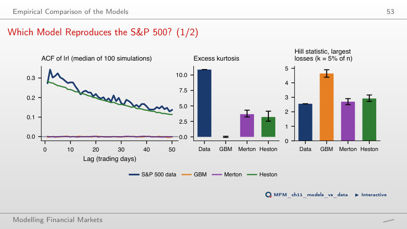
It moves close to zero. Permutation destroys the time ordering responsible for volatility clustering, so the ACF moves close to zero, with sampling fluctuations, as for GBM and Merton. The value 0.28 (the Heston median without permutation, against 0.27 in the data) incorrectly assumes that preserving the empirical distribution also preserves temporal dependence. The excess kurtosis of each simulation remains unchanged. Merton matches the Hill statistic (2.70 against 2.56) and the skewness (−0.32 against −0.36). With these parameters, none of the 100 simulations of the three models reaches the excess kurtosis of the data, 10.88.
Case Studies: Rough and Persistent Volatility, Drift Bursts
Case Study: Replication on SPY, Δ = 1 Day
Answer
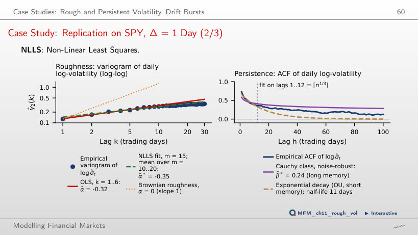
The fit improves at lag 100 but worsens at lag 1. For the plotted curve, A·exp(−κh), the lag-100 value rises from about 0.0014 to 0.073, moving closer to the empirical value of 0.13; at lag 1 it falls from about 0.661 to 0.484, moving away from the empirical value of about 0.73. Fitting more lags does not guarantee improvement at every lag: a single exponential cannot follow both the fast decay at the first lags and the slow tail. The normalized OU benchmark, exp(−κh), is distinct: with the slope fitted over 12 lags (half-life 11 days) it gives 0.002 at lag 100, and with the slope fitted over 60 lags (36 days) it gives 0.149. The Cauchy class gives β̂ = 0.26 and β̂* = 0.24, both below 1, consistent with long memory; the variogram gives α̂ = −0.32 (OLS) and −0.35 (NLLS), a path rougher than Brownian motion.
Second Case Study (2/6): Drift Bursts in SPY, 5-Minute Bars
Answer
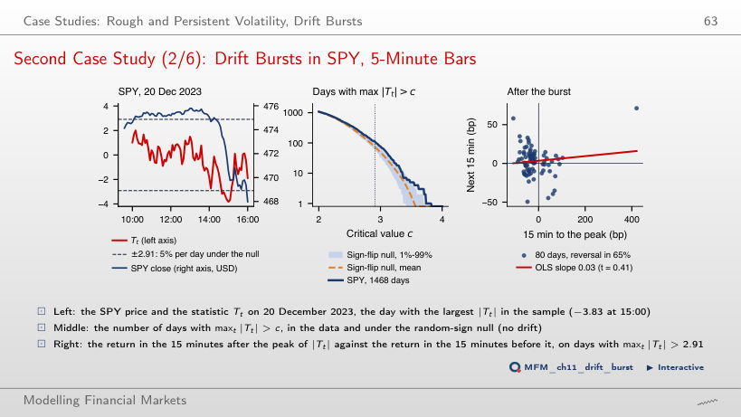
This procedure does not identify the number of true drift bursts. The 109 days are candidates; 109 − 73.84 = 35.16 is a descriptive excess over the random-sign null, which keeps the absolute returns but removes the drift, jump asymmetry and leverage. The threshold is calibrated for approximately 5% daily-maximum exceedances under this null, not for 5% false alarms among selected days or for every process without drift bursts. None of the 200 replications reaches 109 days (the maximum is 100); the Monte Carlo p-value is about 0.005. This result does not identify the mechanism producing the excess. The reversal, present on 65% of the 80 days with a full window after the peak, is descriptive too: the peak is chosen in hindsight, and under the null with the same selection the share is 56.5% on average; the slope is only 0.03, and on E-mini S&P 500 trades the paper finds −0.26.
Daily log returns up to 18 September 2026: S&P 500 (from 1990) and Bitcoin (from 2014), EODHD prices. 3-month US Treasury bill rate: FRED, series DTB3, 1954–2026. Case studies: SPY 5-minute bars, EODHD, October 2020 – September 2026. The simulations (random walk, Brownian motion, GBM, Merton, Heston) use the same seeds as the charts of the lecture.