

The slide of the lecture is on the left, the same figure on the right, computed in the browser from the same data. The ▶ button moves the parameter step by step.
Systemic Risk: from One Bank to the System · Exposure: MES and SRISK · Contribution: CoVaR · Connectedness: Spillover Networks · Tail Networks: the Financial Risk Meter · Stress Testing and Climate Risk · Case Studies: Quantile Connectedness and Bank Fragility
Systemic Risk: from One Bank to the System
Three Banking Systems, 2010–2026
Answer
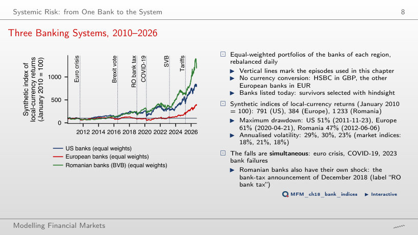
The European portfolio: 61%, with the trough on 2020-04-21. The US portfolio lost 51% up to 2011-11-23 and the Romanian one 47% up to 2012-06-06. The annualised volatility of the bank portfolios is 29%, 30% and 23%, against 18%, 21% and 18% for the S&P 500, Euro Stoxx 50 and BET.
Exposure: MES and SRISK
MES 5% of Thirteen Banks
Answer
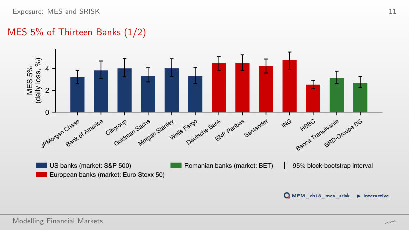
There is no such guarantee. The added days are selected by the market return, not by the bank return, so the MES of a bank need not decrease in α. In this sample it falls for every bank: for JPMorgan, from 3.21% to 2.34%; this is an empirical result, not a general property. At α = 5%, the S&P 500 loses 2.72% on average on those days, and the US banks between 3.21% (JPMorgan) and 4.03% (Morgan Stanley); in Europe, HSBC loses 2.53%, against 3.16% for the Euro Stoxx 50.
SRISK as a Function of Leverage
Answer
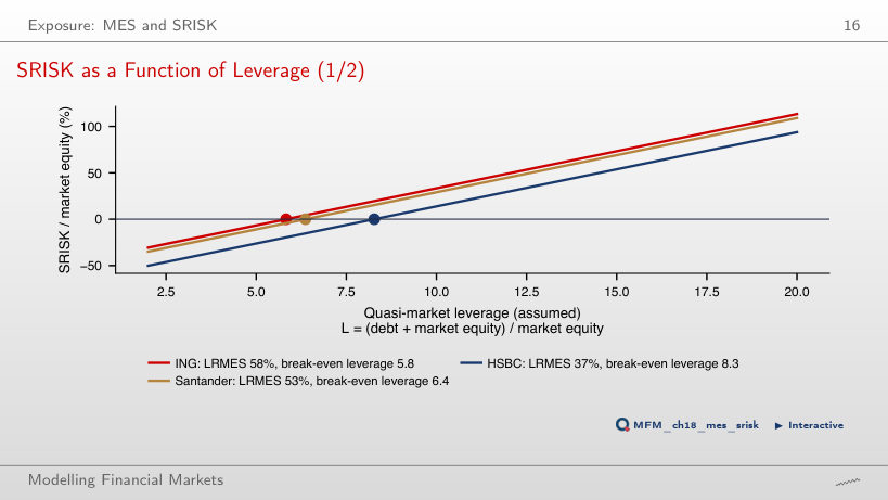
From Λ* = 5.8 with k = 8% and from 8.2 with k = 5.5%. For HSBC, the bank with the lowest LRMES (37%), the thresholds are 8.3 and 11.9. A lower prudential ratio raises the threshold of every bank.
Contribution: CoVaR
Quantile Regression: JPMorgan and the Other US Banks
Answer
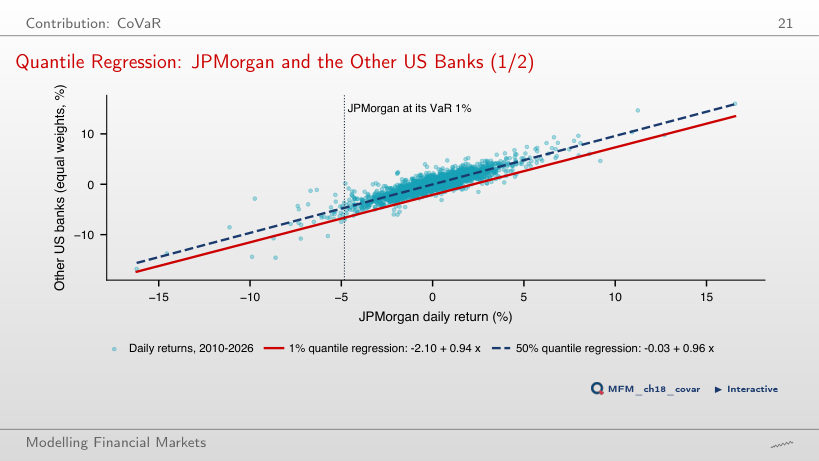
It stays the same: the coefficients are estimated on the full sample and stay fixed; ▶ only changes the visible points and the share of them below the line. The animation is not a recursive estimation. CoVaR 1% is 6.64% with JPMorgan at its VaR 1% (4.83%), against 2.03% with JPMorgan at its median; the difference, ΔCoVaR 1% = 4.62%, is the slope 0.94 times the distance between the two JPMorgan quantiles. The unconditional system VaR 1% is 5.07%.
ΔCoVaR 1% of Eleven Banks
Answer
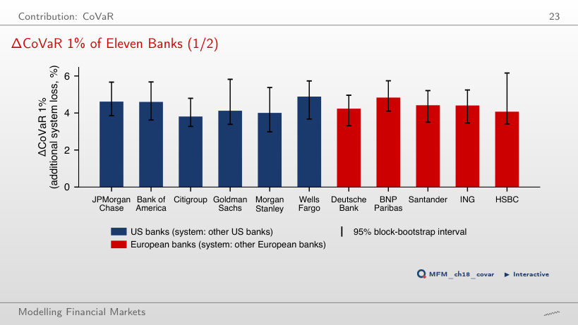
The estimates are 4.89% and 3.81%, but none of the 25 within-region pairs differs after the Holm correction. The overlap of the intervals [3.27, 4.79] and [3.68, 5.73] is not the test. The joint Wald test rejects equal contributions of the US banks (p = 0.011). At α = 5% the ranking changes: its Spearman correlation with the 1% ranking is 0.13.
VaR and ΔCoVaR Measure Different Things
Answer
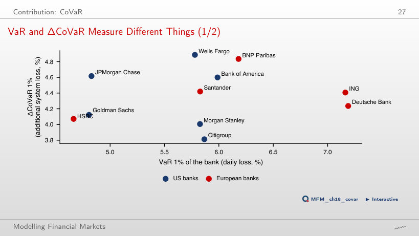
The estimated rank association is weak, without establishing independence. Spearman correlation describes rank association, not independence or a causal effect; 0.13 comes from only 11 banks and is uncertain. At α = 5% the estimate is −0.51: the tail level matters. Deutsche Bank and ING have the largest VaR 1% (7.19% and 7.16%) and only an average ΔCoVaR; JPMorgan has one of the smallest VaR (4.83%) and one of the largest ΔCoVaR (4.62%).
Contribution versus Exposure
Answer
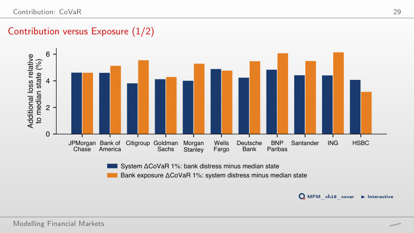
No. Reversing the conditioning requires a separate quantile regression, of the ING return on the system. For ING, the contribution is 4.41% and the exposure 6.14%, both measured against the median state of the conditioning variable; they describe associations in two directions, not causal effects. HSBC is the opposite case: contribution 4.07%, exposure 3.17%. Exposure exceeds contribution for four of the five European banks.
Connectedness: Spillover Networks
The Connectedness Table of Thirteen Banks
Answer
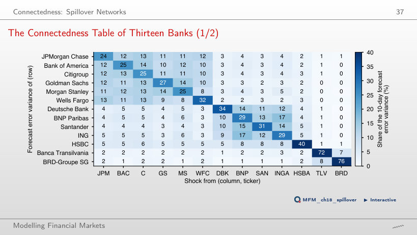
About 57.8% = 84.0 − 26.3: we subtract the own shocks. 84.0% includes the own shocks; 73.7% = 100 − 26.3 includes all the other banks, from every region. The figures are averages over the six US banks. A US bank receives 15.0% from Europe; a European bank receives 72.7% from Europe and 26.2% from the US. Total connectedness, 63.9%, is the average over all banks of the share coming from the other banks. These are normalised shares computed from a VAR(2); residual autocorrelation limits their interpretation as shares of the forecast error variance.
The Net Spillover Network
Answer
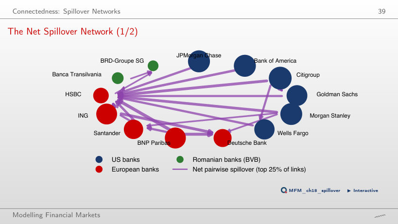
They stay unchanged: net positions are computed from the full matrix, and the threshold only filters the drawing (4 arrows above 3.04 points, instead of 20 above 1.57). Fewer visible arrows do not mean lower estimated connectedness. Transmitters: Citigroup (+19.0), Bank of America (+10.9), Morgan Stanley (+9.9) and JPMorgan (+9.8). Receivers: HSBC (−23.6), BRD (−13.0), Deutsche Bank (−12.6) and Banca Transilvania (−12.2).
Connectedness over Time
Answer
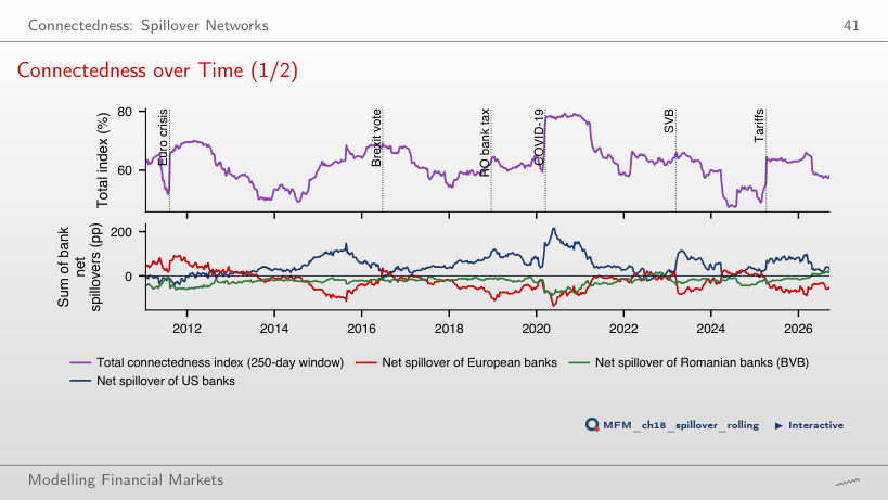
The crisis observations leave the window sooner: each observation stays in the estimation window for fewer days. This can speed up the fall of the index without showing an economic change in transmission. With 250 days, the index rises from 61.8% on average in 2019 to 78.4% in spring 2020, with a maximum of 79.3% on 2020-08-27. With 100 days, the maximum is 85.6% on 2020-03-12, and the index first falls more than 10 points below it on 2020-08-13 (73.4%). There is no general rule for the size of the maximum.
Tail Networks: the Financial Risk Meter
The Financial Risk Meter of Thirteen Banks
Answer
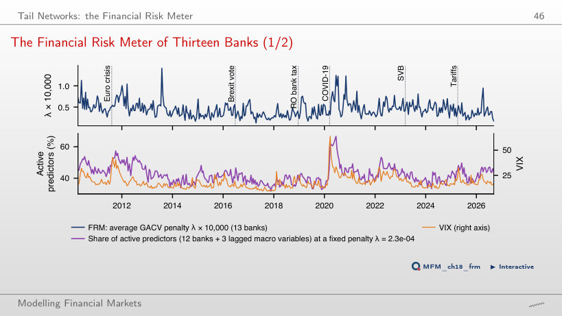
No. The correlations describe simultaneous movement across the 390 windows; they establish neither temporal precedence nor out-of-sample predictive performance. Different units do not prevent the use of a correlation. The share of active predictors at the fixed λ = 2.3 × 10⁻⁴ ranges from 32% (2017-11-20) to 67% (2020-06-16), with a mean of 42%.
Stress Testing and Climate Risk
Seven Historical Stress Scenarios
Answer
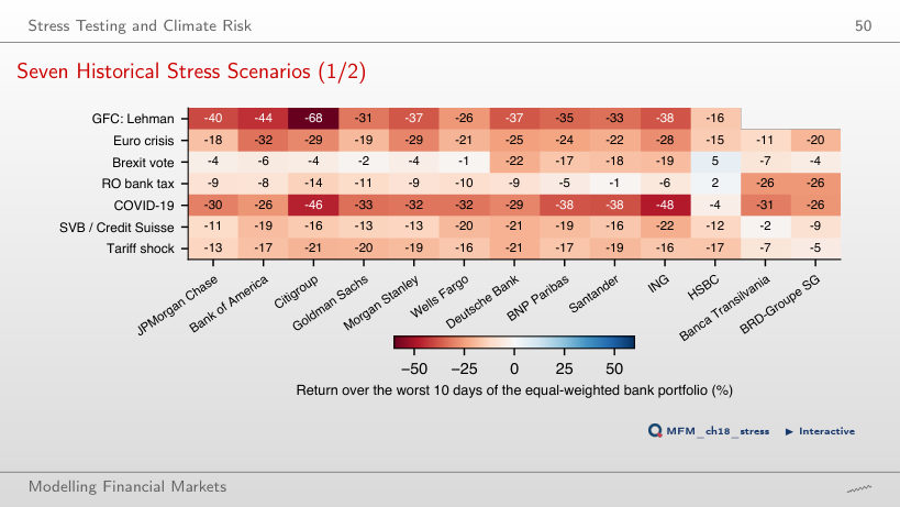
No. For each length the worst window within the episode is searched again, with compounded returns, and the additional days can include recoveries. The Lehman loss falls from 37.6% to 34.8%, while the COVID-19 loss rises from 31.9% to 40.7%. In the Romanian bank-tax episode, with 10 days, Banca Transilvania and BRD lose 26% each, and the US banks between 8% and 14%.
Case Studies: Quantile Connectedness and Bank Fragility
Spillovers across Quantiles
Answer
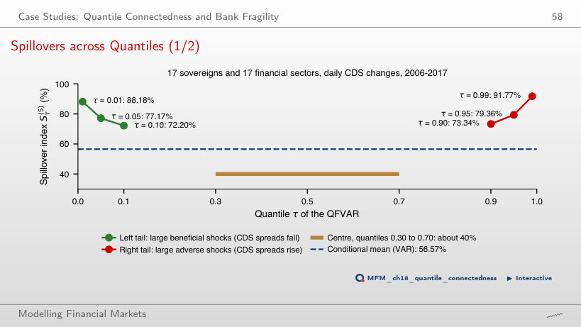
No. RTD = 79.36 − 77.17 = 2.19 points describes the difference between the indices at τ = 0.95 and τ = 0.05; an inferential conclusion requires the estimated uncertainty of the difference. Both tails exceeding the mean index does not test equality between them. The mean index is 56.57%; at τ = 0.01 and 0.99 it is 88.18% and 91.77%, and in the centre about 40%.
Treasuries and Bank Equity, 2022–2023
Answer
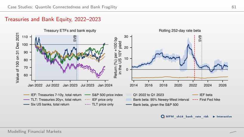
We do not reject a zero beta, although the point estimate is positive: the interval contains zero, so the test does not establish the sign of the coefficient at 5%; this does not mean that beta is zero. At the end of 2021 the estimate was +12.8%. These are associations conditional on the S&P 500 return, per 100 bp rise in the 10-year yield. Separately, the IEF beta, −7.8% per +100 bp, is estimated over 3 January 2022 – 9 March 2023. From 31 December 2021 to 31 March 2023, the IEF price fell by 13.8% and the TLT price by 28.2% (total returns: −11.8% and −26.2%).
Daily EODHD prices, January 2010 to 18 September 2026: six US banks, five European banks, two Romanian banks (BVB), the S&P 500, Euro Stoxx 50, BET and VIX indices. The historical scenarios for the international banks start in 2007. First case study: values reported by Ando, Greenwood-Nimmo and Shin (2022). Second case study: the IEF and TLT ETFs and the US 10-year Treasury yield (EODHD), from September 2012.