Neural Networks and Deep Learning

Lecture 13: Deep learning for energy and financial time series; time-series foundation models

Lecture 13

Deep learning for energy and financial time series; time-series foundation models

Prof. dr. Daniel Traian PELE

Bucharest University of Economic Studies (ASE), Department of Statistics and Econometrics
Romanian Academy, Institute for Economic Forecasting (IPE)

Every day before noon, a Romanian electricity supplier, a hydro producer or a battery operator sends bids for each hour of the next day, and every day a bank reports the loss its portfolio should exceed only once in a hundred days. Both decisions need a forecast: a price for each of the 24 hours of tomorrow, or a quantile of tomorrow's return. This lecture asks a simple question on real data: do neural networks trained on our own series, or the new time-series foundation models pre-trained on millions of other series, beat the simple benchmarks that practitioners already use?

We forecast Romanian day-ahead electricity prices for a full test year (1 November 2025 to 31 October 2026, 364 complete days) with nine strategies: a naive rule, the Lasso-estimated autoregressive model (LEAR), a deep neural network (DNN) with 24 outputs, the neural basis expansion analysis (N-BEATS), three foundation models used zero-shot (Chronos-2, Chronos-Bolt and the Time-series Foundation Model, TimesFM), Chronos-2 with covariates and a simple ensemble. We then turn the foundation model's quantiles into calibrated intervals with conformal prediction, and use the same idea for the Value-at-Risk (VaR) of the S&P 500 and of Bitcoin.

What you will be able to do

  • Set up a day-ahead forecasting problem without leakage: information set at gate closure, rolling origin, benchmarks.
  • Write and estimate LEAR, a DNN with 24 outputs and N-BEATS on Romanian prices.
  • Explain how time-series foundation models forecast without any training on our data, and test them.
  • Compare forecasts with the Diebold–Mariano test and calibrate probabilistic forecasts with conformal prediction.
  • Use a foundation model for Value-at-Risk and backtest it.

Lecture plan

  1. The forecasting problem and the dataA forecast is only as good as the information it is allowed to use.
  2. A strong linear benchmark and a deep networkBefore a deep network, a strong linear benchmark: LEAR is the open reference model of electricity price forecasting.
  3. Deep forecasting architecturesThree ideas shape modern forecasting networks: a recurrent network that outputs a distribution (DeepAR), stacks of fully connected blocks (N-BEATS), and transformers on patches of the series.
  4. Time-series foundation modelsA foundation model is pre-trained once on a very large collection of series and then used as it is: it reads our context and returns quantiles, with no gradient step on our data.
  5. Probabilistic forecasts and conformal calibrationA battery operator or a risk desk needs the distribution of tomorrow's price, not just its centre.
  6. Foundation models for financial riskThe same quantile machinery gives a Value-at-Risk.

The forecasting problem and the data

A forecast is only as good as the information it is allowed to use. This section describes the data, the stylised facts of Romanian power prices and the rules of the game: what is known when the auction closes, how the test year is kept untouched, and which benchmark every model has to beat.

Two business decisions based on day-ahead forecasts

Slide 6 in the PDF

On the day-ahead market, the price of every hour of tomorrow is set by one auction coupled across Europe and run in Romania by the Romanian electricity and gas market operator (OPCOM). Bids close at 12:00 Central European Time (CET) on the day before delivery. An error of 1 EUR/MWh on 100 MW over 24 hours costs 2,400 euro per day, so even small improvements matter. In finance, the Value-at-Risk is the quantile of tomorrow's return that should be breached on 1 % of days; under the Basel rules the number of breaches in a year moves the capital charge.
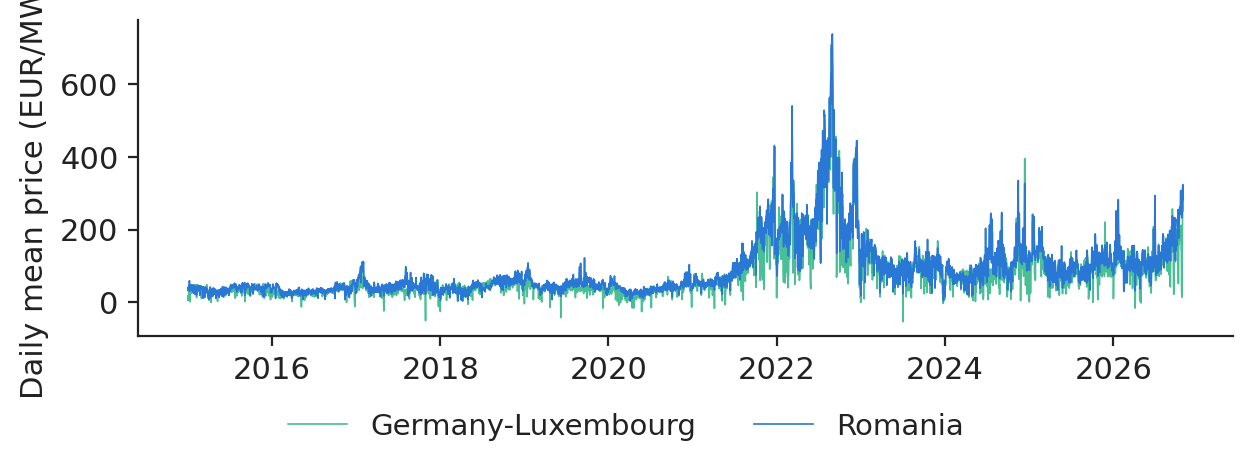

Prices for Romania (RO), Germany–Luxembourg (DE-LU) and Hungary (HU) and the Romanian load come from energy-charts.info, the data portal of the Fraunhofer Institute for Solar Energy Systems (ISE), which republishes exchange data and the data of the European Network of Transmission System Operators for Electricity (ENTSO-E). The price file runs from 1 January 2015 to 31 October 2026 with 103,595 hourly prices. Daily closes of the S&P 500 and of Bitcoin come from Yahoo Finance. Missing hours stay missing: the two clock-change days of every year enter only if all 24 hours exist.

Daily mean day-ahead prices in Romania

Slide 8 in the PDF
Chart: Daily mean day-ahead prices in Romania

Daily mean day-ahead prices in Romania and Germany–Luxembourg.

Source: energy-charts.info (Fraunhofer ISE), from exchange and ENTSO-E data. Data: 1 Jan 2015 to 31 Oct 2026, daily means of hourly prices.

The mean Romanian price was 50.41 EUR/MWh in 2019 and 265.31 EUR/MWh in 2022; the highest daily mean, 738.28 EUR/MWh, was reached on 30 August 2022. The daily means of Romania and Germany move together (correlation 0.936), which is why German prices are useful inputs. A model trained only before 2021 has never seen prices like those of 2022, and a model trained mostly on 2022 overestimates today's prices: the training window is a modelling decision. We use three years, as in Lago et al. (2021).

Solar power has turned the midday peak into a trough

Slide 9 in the PDF
Chart: Solar power has turned the midday peak into a trough

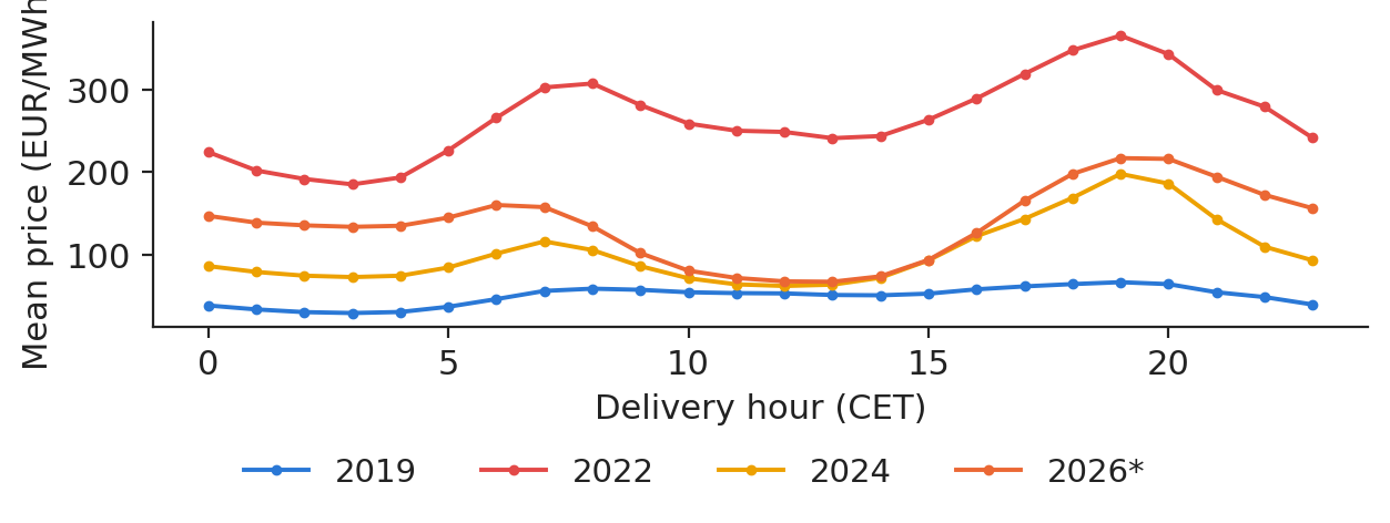
Mean price by delivery hour, selected years.

Source: energy-charts.info (Fraunhofer ISE), from exchange and ENTSO-E data. Data: 2019, 2022, 2024 and 2026 (*January-October), Romania.

In 2019 the cheapest hour was the night; in 2026 (January–October) the cheapest hour is 13:00, at 67.90 EUR/MWh, while the evening hour 19:00 is the most expensive, at 217.05 EUR/MWh. The forecaster has to predict 24 different hours with different dynamics, which is why every model below has 24 outputs.

Information set at gate closure

Slide 10 in the PDF

For delivery day \(d\), a model may use only what is known before 12:00 CET on day \(d-1\):

\[\hat{\mathbf y}_d=f_{\boldsymbol\theta}(\mathbf x_d),\qquad \mathbf x_d=(\mathbf y_{d-1},\mathbf y_{d-2},\mathbf y_{d-3},\mathbf y_{d-7},\mathbf y^{\text{DE}}_{d-1},\boldsymbol\ell_{d-2},\mathbf c_d)\]

where \(\mathbf y_d\in\mathbb R^{24}\) are the Romanian prices of day \(d\), \(\mathbf y^{\text{DE}}\) the German prices, \(\boldsymbol\ell\) the Romanian load (complete two days back) and \(\mathbf c_d\) day-of-week dummies. This gives 151 inputs and 3,819 daily samples since 2016. Models are re-estimated on a rolling window of 1,092 days and the test year is used once.

In practice: the load of day \(d-1\) is not complete at noon; using it would leak the future into the forecast.

Error measures and the benchmark model

Slide 11 in the PDF

We report the mean absolute error (MAE) in EUR/MWh and the relative MAE, \(\mathrm{rMAE}=\mathrm{MAE}/\mathrm{MAE}^{\text{naive}}\), where the naive forecast is the price of the same hour one week earlier for Monday, Saturday and Sunday and the price of the day before otherwise. Percentage errors are useless when prices are close to zero or negative; in the test year there were 195 negative hours, the mean price was 134.59 EUR/MWh and the naive forecast reached an MAE of 27.74 EUR/MWh.

Section summary

The rules of the game: information at gate closure only, a rolling window, one untouched test year, and the naive forecast as the floor.

A strong linear benchmark and a deep network

Before a deep network, a strong linear benchmark: LEAR is the open reference model of electricity price forecasting. The DNN uses exactly the same inputs, so the comparison isolates the model.

Variance-stabilising transform

Slide 13 in the PDF

Prices have spikes and can be negative. The area hyperbolic sine behaves like a logarithm for large values and like the identity near zero:

\[z=\operatorname{asinh}\Big(\frac{y-\tilde m}{\hat\sigma}\Big),\qquad \hat\sigma=\frac{\mathrm{MAD}}{0.6745}\]

with \(\tilde m\) the median and MAD the median absolute deviation of the training window (Uniejewski, Weron & Ziel, 2018). Forecasts are made on the transformed scale and transformed back with \(y=\tilde m+\hat\sigma\sinh(\hat z)\).

LEAR: 24 Lasso regressions, one per hour

Slide 14 in the PDF
\[\hat{\boldsymbol\beta}_h=\arg\min_{\boldsymbol\beta}\sum_{d\in W}\big(z_{d,h}-\mathbf x_d^{\top}\boldsymbol\beta\big)^2+\lambda_h\lVert\boldsymbol\beta\rVert_1\]

with \(\lambda_h\) chosen by the Akaike information criterion (AIC) on the Lasso path and re-estimated every day. On our test year LEAR reaches an MAE of 22.79 EUR/MWh (rMAE 0.822).

The DNN: one network, 24 outputs

Slide 15 in the PDF

A multilayer perceptron (MLP) maps the inputs to the 24 hours at once:

\[\hat{\mathbf z}_d=\mathbf W_3\,\mathrm{ReLU}\big(\mathbf W_2\,\mathrm{ReLU}(\mathbf W_1\mathbf x_d+\mathbf b_1)+\mathbf b_2\big)+\mathbf b_3,\qquad z_{d,h}=\operatorname{asinh}\frac{y_{d,h}-m_d}{s_d}\]

where \(m_d\) is the median price of day \(d-1\) and \(s_d\) a robust scale of the lagged prices, so each day is put on its own level (instance normalisation). The network has 256 and 128 hidden units (74,904 parameters), dropout 0.1, the L1 loss and early stopping on the last 20 % of the window; it is recalibrated monthly with 4 seeds. Its test MAE is 23.06 EUR/MWh; single seeds range from 23.57 to 24.03.

Early stopping

Slide 16 in the PDF
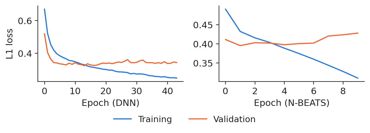
Chart: Early stopping picks the epoch on data the network did not train on

Training and validation loss of the DNN and of N-BEATS.

Source: energy-charts.info (Fraunhofer ISE), from exchange and ENTSO-E data. Data: training windows before 1 Nov 2025, Romania.

The validation loss of the DNN is lowest at epoch 14 of 44; N-BEATS, trained on many more hourly windows, stops improving after epoch 2.

Section summary

LEAR and the DNN use the same information; the DNN does not beat LEAR by a significant margin on this year, a common finding in the literature.

Deep forecasting architectures

Three ideas shape modern forecasting networks: a recurrent network that outputs a distribution (DeepAR), stacks of fully connected blocks (N-BEATS), and transformers on patches of the series.

A probabilistic recurrent network

Slide 18 in the PDF

The deep autoregressive recurrent network (DeepAR) of Salinas et al. (2020) runs a long short-term memory network (LSTM) over the series and outputs the parameters of tomorrow's distribution; it is trained by maximum likelihood on many related series at once. Its global, probabilistic design is the ancestor of today's foundation models.

N-BEATS: blocks that explain the input and forecast the rest

Slide 19 in the PDF

Each block reads the residual of the input, removes what it can explain (the backcast) and adds its share to the forecast:

\[\mathbf r_\ell=\mathbf r_{\ell-1}-\hat{\mathbf r}_\ell,\qquad \hat{\mathbf y}=\sum_{\ell=1}^{L}\hat{\mathbf y}_\ell\]

Our N-BEATS reads the last 168 hours of prices only, has 6 blocks and 1,739,904 parameters, and was trained once before the test year: test MAE 23.23 EUR/MWh (three seeds from 23.69 to 24.12).

Transformers for time series: patches as tokens

Slide 20 in the PDF

The patch time-series transformer (PatchTST) cuts the series into patches of, say, 16 hours, embeds each patch like a word and applies attention across patches. A context of 2,048 hours becomes 128 tokens, so the attention cost falls 256 times. The foundation models below are built on this idea.

Time-series foundation models

A foundation model is pre-trained once on a very large collection of series and then used as it is: it reads our context and returns quantiles, with no gradient step on our data.

A foundation model forecasts a series it has never seen

Slide 22 in the PDF
\[\hat q^{\tau}_{T+k}=g_{\boldsymbol\theta^{*}}\big(y_{T-C+1:T}\big)_{k,\tau}\]

where \(C\) is the context length (2,048 hours here), \(\tau\) a quantile level and \(\boldsymbol\theta^{*}\) the frozen pre-trained weights, obtained by minimising the quantile (pinball) loss over the pre-training corpus. We test Chronos-2 and Chronos-Bolt (Amazon) and TimesFM 2.5 (Google Research).

Chronos: tokenisation of time series

Slide 23 in the PDF

The original Chronos (Ansari et al., 2024) divides the series by its mean absolute value, cuts the scaled values into bins and trains a language model to predict the next bin with the cross-entropy loss. Chronos-Bolt and Chronos-2 replace the bins by patches and quantile outputs. The model knows shapes (seasonality, mean reversion), not the Romanian market.

Test-year accuracy

Slide 24 in the PDF
ModelMAE (EUR/MWh)rMAE
Naive27.741.000
LEAR22.790.822
DNN23.060.831
N-BEATS23.230.837
Chronos-Bolt21.670.781
TimesFM 2.522.370.806
Chronos-220.720.747
Chronos-2 + covariates20.410.736
Ensemble LEAR + DNN + Chronos-220.770.749

Trained networks versus zero-shot foundation models

Slide 25 in the PDF
Chart: Trained networks versus zero-shot foundation models

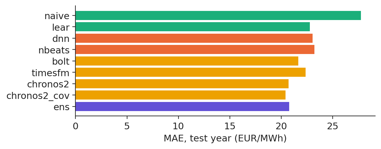
Mean absolute error of the nine forecasts on the test year.

Source: energy-charts.info (Fraunhofer ISE), from exchange and ENTSO-E data. Data: 1 Nov 2025 to 31 Oct 2026, 360 days x 24 hours, Romania.

The zero-shot Chronos-2 forecast, with no training on Romanian data, has a lower MAE (20.72 EUR/MWh) than LEAR (22.79) and the two networks trained here. Adding the German and Hungarian prices and the Romanian load as past covariates lowers it further, to 20.41 EUR/MWh.

In practice: start with the benchmark and a foundation model: both cost minutes, not weeks.

Errors by hour

Slide 26 in the PDF
Chart: Errors are largest in the evening and around solar hours

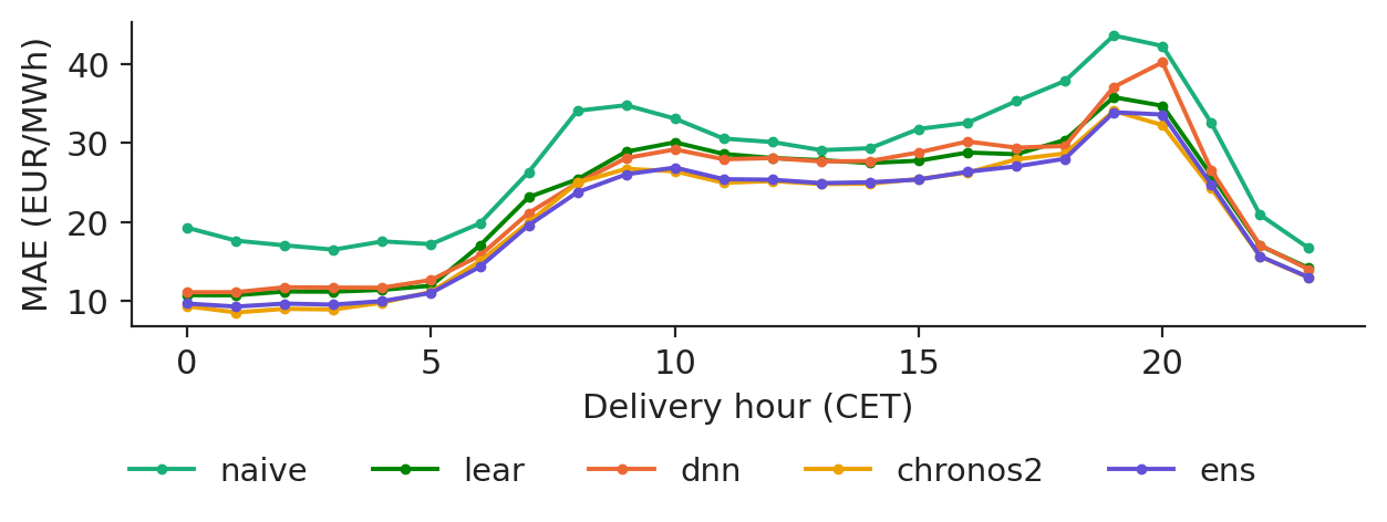
MAE by delivery hour.

Source: energy-charts.info (Fraunhofer ISE), from exchange and ENTSO-E data. Data: 1 Nov 2025 to 31 Oct 2026, 360 days x 24 hours, Romania.

All models struggle in the evening: the worst hour of LEAR is 19:00 (MAE 35.78 EUR/MWh) and so is that of Chronos-2 (34.05), while night hours are forecast within about 10.75 EUR/MWh.

One week of forecasts

Slide 27 in the PDF
Chart: Forecasts for one week of the test year

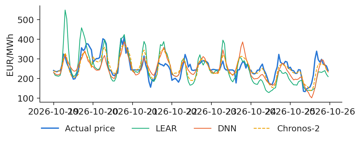
Actual prices and three forecasts, 19–25 October 2026.

Source: energy-charts.info (Fraunhofer ISE), from exchange and ENTSO-E data. Data: 19 Oct 2026 to 25 Oct 2026, hourly, Romania.

In the week of 19 October 2026 to 25 October 2026 the MAE was 43.34 for LEAR, 32.33 for the DNN and 25.41 EUR/MWh for Chronos-2. All models follow the daily shape and smooth the evening spikes.

Effect of context length

Slide 28 in the PDF
Chart: Effect of context length on the foundation model

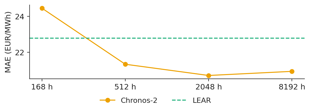
Chronos-2 MAE as a function of the context length.

Source: energy-charts.info (Fraunhofer ISE), from exchange and ENTSO-E data. Data: 1 Nov 2025 to 31 Oct 2026, 360 days x 24 hours, Romania.

With one week of context (168 hours) the MAE of Chronos-2 is 24.45 EUR/MWh; with 2,048 hours it falls to 20.72, and 8,192 hours do not help further (20.95). The context length is the main tuning knob of a zero-shot model.

The Diebold–Mariano test

Slide 29 in the PDF

A lower average error can be luck. With the daily loss differential \(\Delta_d=\lVert\mathbf e^{A}_d\rVert_1-\lVert\mathbf e^{B}_d\rVert_1\) over the 24 hours of each day,

\[\mathrm{DM}=\frac{\bar\Delta}{\hat\sigma_\Delta/\sqrt{|\mathcal T|}}\ \overset{a}{\sim}\ \mathcal N(0,1)\]

tests whether model B is more accurate than model A (Diebold & Mariano, 1995; Ziel & Weron, 2018). Working with daily rather than hourly losses respects the fact that the 24 hours of a day share the same information.

Pairwise Diebold–Mariano tests

Slide 30 in the PDF
Chart: Pairwise Diebold–Mariano tests for all models

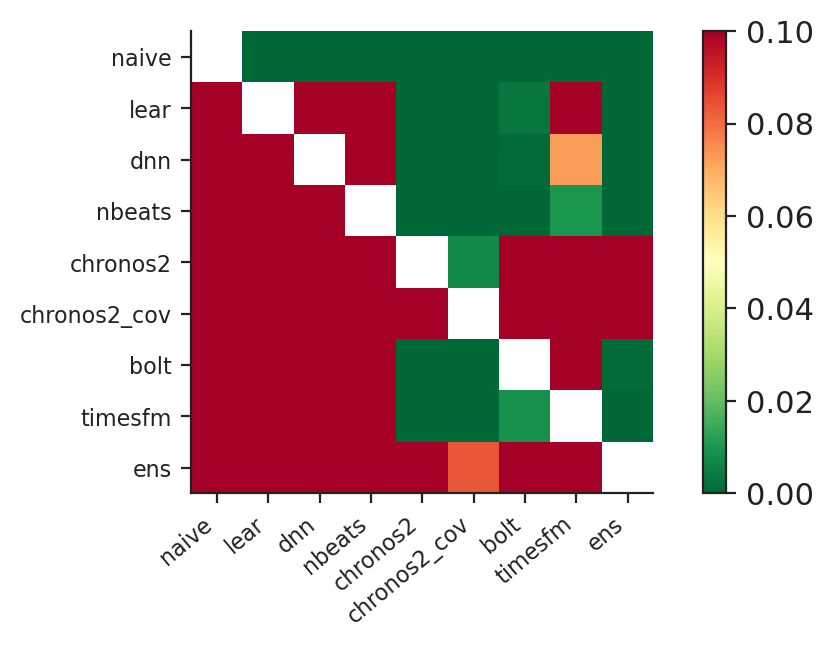
One-sided p-values of the multivariate Diebold–Mariano test.

Source: energy-charts.info (Fraunhofer ISE), from exchange and ENTSO-E data. Data: 1 Nov 2025 to 31 Oct 2026, 360 days x 24 hours, Romania.

Chronos-2 is significantly more accurate than LEAR (p < 0.001), and so is the ensemble, while the DNN is not significantly better than LEAR (p = 0.761). Adding covariates to Chronos-2 is a significant improvement (p = 0.007).

Section summary

Foundation models forecast Romanian prices zero-shot as well as, or better than, models trained here; significance must be tested on daily losses.

Probabilistic forecasts and conformal calibration

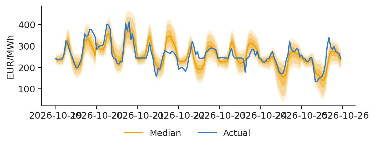
A battery operator or a risk desk needs the distribution of tomorrow's price, not just its centre. Foundation models output quantiles directly; conformal prediction makes them reliable.

Quantile forecasts and the pinball loss

Slide 33 in the PDF

A quantile forecast \(\hat q^{\tau}\) is scored with the pinball loss \(\rho_\tau(u)=u(\tau-\mathbb 1\{u<0\})\), \(u=y-\hat q^{\tau}\), averaged over the nine deciles. On the test year: Chronos-2 8.25, with covariates 8.11, Chronos-Bolt 8.62, TimesFM 8.97 and LEAR with empirical errors 9.12 EUR/MWh.

Split-conformal correction

Slide 35 in the PDF

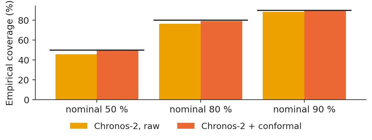
The conformity score of each past hour measures how far the outcome fell outside the raw band, \(s_i=\max(\hat q^{\alpha/2}_i-y_i,\ y_i-\hat q^{1-\alpha/2}_i)\). Taking the \(\lceil (n+1)(1-\alpha)\rceil\)-th smallest score of the last 60 days as \(\hat Q\) and widening the band by \(\hat Q\) on both sides guarantees coverage of at least \(1-\alpha\) when the data are exchangeable (Romano, Patterson & Candès, 2019); for time series the guarantee is approximate. For the 80 % band, the raw Chronos-2 coverage was 76.5 % and the conformal coverage 79.3 %, with the mean width moving from 60.03 to 63.89 EUR/MWh.

Coverage against the nominal level

Slide 36 in the PDF
Chart: Conformal calibration moves coverage towards the nominal level

Empirical coverage of 50, 80 and 90 % intervals.

Source: energy-charts.info (Fraunhofer ISE), from exchange and ENTSO-E data. Data: 1 Nov 2025 to 31 Oct 2026, 360 days x 24 hours, Romania.

For the 90 % band: raw 88.3 %, conformal 89.4 %, LEAR with empirical errors 85.0 %.

Load forecasts of foundation models

Slide 37 in the PDF
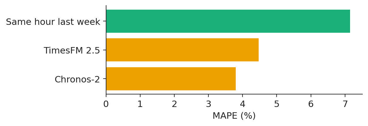
Chart: Load forecasts of foundation models: errors of a few percent

Mean absolute percentage error of hourly Romanian load forecasts.

Source: energy-charts.info (Fraunhofer ISE), from exchange and ENTSO-E data. Data: 1 Nov 2025 to 31 Oct 2026, 360 days, Romanian load.

For the Romanian load (mean 5,932 MW), percentage errors are meaningful: the same hour of last week gives a mean absolute percentage error (MAPE) of 7.15 %, TimesFM 4.47 % and Chronos-2 3.80 %.

Foundation models for financial risk

The same quantile machinery gives a Value-at-Risk.

Value-at-Risk and its backtest

Slide 39 in the PDF

The one-day VaR at level \(\alpha\) is the conditional \(\alpha\)-quantile of tomorrow's return. The Kupiec test compares the share of violations with \(\alpha\),

\[\mathrm{LR}_{uc}=-2\ln\frac{(1-\alpha)^{n_0}\alpha^{n_1}}{(1-\hat\pi)^{n_0}\hat\pi^{n_1}}\sim\chi^2_1\]

and the Christoffersen test checks that violations do not cluster. We compare historical simulation (HS), a GARCH(1,1) model with Student-\(t\) errors and Chronos-2 quantiles from the last 1,024 returns.

A one-sided conformal shift

Slide 40 in the PDF

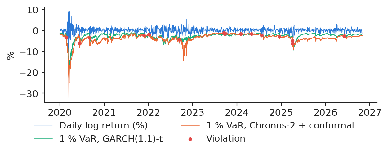
With \(s_i=\hat q^{\alpha}_i-r_i\) over the last 250 days and \(c_t\) its \(\lceil (n+1)(1-\alpha)\rceil\)-th smallest value, the calibrated VaR is \(\hat q^{\alpha}_{t+1}-c_t\). On the S&P 500 at the 1 % level, the raw Chronos-2 quantile was breached 22 times, the conformal one 16 times, against 17.2 expected.

The calibrated VaR follows volatility regimes

Slide 41 in the PDF
Chart: S&amp;P 500: the calibrated foundation-model VaR follows volatility regimes

S&P 500 returns with the 1 % VaR of GARCH(1,1)-t and of Chronos-2 with a conformal shift.

Source: Yahoo Finance, daily quotes. Data: 2 Jan 2020 to 30 Oct 2026, trading days, S&P 500.

Over 1,717 trading days the conformal Chronos-2 VaR passed the Kupiec test at both levels (p = 0.774 at 1 % and 0.434 at 5 %), while GARCH was breached 32 times at 1 % (p = 0.001). For Bitcoin, all methods give acceptable 1 % coverage; the conformal Chronos-2 VaR had 21 violations against 25.0 expected.

In practice: recalibration is a model change: document it and backtest it out of sample.

Quantile forecasts from language models and time-series models

Slide 43 in the PDF

Lecture 12 wrote past returns into the prompt of a language model (LLM-VaR, Pele et al., 2026); here a time-series foundation model reads them as numbers. Both are zero-shot, both must be backtested out of sample against GARCH and historical simulation.

Section summary

The foundation-model route gives quantiles in seconds; conformal calibration and standard backtests make them usable for risk.

Videos: the intuition behind the mathematics (in English)

Abbreviations

AICAkaike information criterion
ASEBucharest University of Economic Studies
CETCentral European Time
CQRconformalised quantile regression
DE-LUGermany–Luxembourg bidding zone
DeepARdeep autoregressive recurrent network (Salinas et al., 2020)
DMDiebold–Mariano test
DNNdeep neural network (here: a multilayer perceptron with 24 outputs)
ENTSO-EEuropean Network of Transmission System Operators for Electricity
ESexpected shortfall
EUReuro
GARCHgeneralised autoregressive conditional heteroskedasticity
HShistorical simulation
HUHungary (bidding zone)
IPEInstitute for Economic Forecasting, Romanian Academy
ISEFraunhofer Institute for Solar Energy Systems
LEARLasso-estimated autoregressive model
LLMlarge language model
LRlikelihood ratio
LSTMlong short-term memory network
MADmedian absolute deviation
MAEmean absolute error
MAPEmean absolute percentage error
MLPmultilayer perceptron
MWmegawatt
MWhmegawatt-hour
N-BEATSneural basis expansion analysis for time series
OPCOMRomanian electricity and gas market operator
PatchTSTpatch time-series transformer
ReLUrectified linear unit
RMSEroot mean squared error
RORomania (bidding zone)
TimesFMTime-series Foundation Model (Google Research)
VaRValue-at-Risk

References

  • Andrei, A.-V., Pele, D.-T., Cramer, A.-A., Amza, A. & Diaconu, D. (2026). Explainable AI-based early warning system for electricity price spikes: Evidence from the Romanian market. Proceedings of the International Conference on Business Excellence, 20(1), 4820–4836. doi:10.2478/picbe-2026-0352
  • Andrei, A.-V., Pele, D.-T. & Cramer, A.-A. (2026). Multi-horizon explainability in energy price forecasting: Disentangling market dynamics and renewable intermittency in Romania's liberalized electricity market. Proceedings of the International Conference on Business Excellence, 20(1), 104–117. doi:10.2478/picbe-2026-0014
  • Andrei, A.-V., Velev, G., Toma, F.-M., Pele, D. T. & Lessmann, S. (2024). Energy price modelling: A comparative evaluation of four generations of forecasting methods. arXiv:2411.03372
  • Ansari, A. F. et al. (2024). Chronos: Learning the language of time series. Transactions on Machine Learning Research. arXiv:2403.07815
  • Ansari, A. F. et al. (2025). Chronos-2: From univariate to universal forecasting. arXiv:2510.15821
  • Będowska-Sójka, B., Wójcik, P. & Pele, D. T. (2026). Early warning systems for cryptocurrency markets: Predicting `zombie' assets using machine learning. The North American Journal of Economics and Finance, 81, 102543. doi:10.1016/j.najef.2025.102543
  • Christoffersen, P. F. (1998). Evaluating interval forecasts. International Economic Review, 39(4), 841–862. doi:10.2307/2527341
  • Das, A., Kong, W., Sen, R. & Zhou, Y. (2024). A decoder-only foundation model for time-series forecasting. Proceedings of the 41st International Conference on Machine Learning. arXiv:2310.10688
  • Diebold, F. X. & Mariano, R. S. (1995). Comparing predictive accuracy. Journal of Business & Economic Statistics, 13(3), 253–263. doi:10.1080/07350015.1995.10524599
  • Kupiec, P. H. (1995). Techniques for verifying the accuracy of risk measurement models. The Journal of Derivatives, 3(2), 73–84. doi:10.3905/jod.1995.407942
  • Lago, J., Marcjasz, G., De Schutter, B. & Weron, R. (2021). Forecasting day-ahead electricity prices: A review of state-of-the-art algorithms, best practices and an open-access benchmark. Applied Energy, 293, 116983. doi:10.1016/j.apenergy.2021.116983
  • Nie, Y., Nguyen, N. H., Sinthong, P. & Kalagnanam, J. (2023). A time series is worth 64 words: Long-term forecasting with transformers. International Conference on Learning Representations. arXiv:2211.14730
  • Oreshkin, B. N., Carpov, D., Chapados, N. & Bengio, Y. (2020). N-BEATS: Neural basis expansion analysis for interpretable time series forecasting. International Conference on Learning Representations. arXiv:1905.10437
  • Pele, D. T., Bolovăneanu, V., Lin, M.-B., Ren, R., Ginavar, A. T., Spilak, B., Andrei, A.-V., Toma, F.-M., Lessmann, S. & Härdle, W. K. (2026). In the beginning was the Word: LLM-VaR and LLM-ES. Expert Systems with Applications, 295, 128676. doi:10.1016/j.eswa.2025.128676
  • Romano, Y., Patterson, E. & Candès, E. (2019). Conformalized quantile regression. Advances in Neural Information Processing Systems, 32. arXiv:1905.03222
  • Salinas, D., Flunkert, V., Gasthaus, J. & Januschowski, T. (2020). DeepAR: Probabilistic forecasting with autoregressive recurrent networks. International Journal of Forecasting, 36(3), 1181–1191. doi:10.1016/j.ijforecast.2019.07.001
  • Uniejewski, B., Weron, R. & Ziel, F. (2018). Variance stabilizing transformations for electricity spot price forecasting. IEEE Transactions on Power Systems, 33(2), 2219–2229. doi:10.1109/TPWRS.2017.2734563
  • Weron, R. (2014). Electricity price forecasting: A review of the state-of-the-art with a look into the future. International Journal of Forecasting, 30(4), 1030–1081. doi:10.1016/j.ijforecast.2014.08.008
  • Ziel, F. & Weron, R. (2018). Day-ahead electricity price forecasting with high-dimensional structures: Univariate vs. multivariate modeling frameworks. Energy Economics, 70, 396–420. doi:10.1016/j.eneco.2017.12.016

Text written for the web version of the lecture; numbers, charts and sources come from the slides and their Quantlets.