Neural Networks and Deep Learning

Lecture 9: Graph neural networks

Lecture 9

Graph neural networks

Prof. dr. Daniel Traian PELE

Bucharest University of Economic Studies (ASE), Department of Statistics and Econometrics
Romanian Academy, Institute for Economic Forecasting (IPE)

Money laundering is rarely visible in a single payment. It shows in the chain: funds split across many addresses, passed through intermediaries and merged again. Banks, payment processors and crypto exchanges therefore look at transactions as a network, and graph neural networks (GNN) are the deep-learning tool built for that view: each transaction learns from its neighbours, its neighbours' neighbours, and so on.

This lecture builds the three classic GNN layers, the graph convolutional network (GCN), graph sample and aggregate (GraphSAGE) and the graph attention network (GAT), and tests them for anti-money laundering (AML) on the Elliptic graph of 203,769 Bitcoin transactions released by Weber et al. (2019), against a logistic regression and a random forest, in time order and with the measures that matter to an investigation team.

What you will be able to do

  • Represent financial data as a graph: nodes, edges, features, adjacency and normalised adjacency.
  • Write the message-passing scheme and the GCN, GraphSAGE and GAT layers with every symbol defined.
  • Train them on the Elliptic graph in time order, against strong non-graph benchmarks.
  • Judge the results with precision, recall, the area under the precision-recall curve (PR-AUC), alert budgets, drift and the stability of explanations.

Lecture plan

  1. Graphs in the detection of financial crimeThe Elliptic graph shows what a transaction network looks like and why the neighbours carry information.
  2. Graphs as matricesAdjacency, degree and the Laplacian turn a graph into linear algebra.
  3. Message passingEvery GNN layer collects messages from the neighbours, aggregates them and updates the node.
  4. GCN, GraphSAGE and GATThree choices of message, aggregation and update, from fixed degree weights to learned attention.
  5. Case study: illicit Bitcoin transactionsEight models on the same temporal test, judged like an investigation team would judge them.
  6. GNNs in productionGraph models in finance fail in specific ways; knowing them is part of the model.

Graphs in the detection of financial crime

The Elliptic graph shows what a transaction network looks like and why the neighbours carry information.

Network structure in money-laundering detection

Slide 5 in the PDF

A graph \(G=(\mathcal V,\mathcal E,\mathbf X)\) has nodes \(\mathcal V\) (here transactions), edges \(\mathcal E\) (a payment flow from one transaction to the next) and a feature matrix \(\mathbf X\in\mathbb R^{n\times d}\); the label \(y_v=1\) marks an illicit transaction (scams, ransomware, dark markets). The Elliptic graph has 203,769 transactions, 234,355 payment flows, 165 features per transaction and 49 time steps. The task is node classification.

In practice: a bank's anti-money-laundering team already thinks in chains of payments; a GNN learns from the same chains.

Description of the Elliptic data set

Slide 6 in the PDF
ElementValue
Labels4,545 illicit, 42,019 licit, 157,205 unknown (22.9 % labelled)
Features93 local + 72 aggregated over the neighbours
Time49 steps of about two weeks; 100.0 % of the edges join transactions of the same step
Training / teststeps 1–34 (29,894 labelled) / steps 35–49 (16,670 labelled, 1,083 illicit)

Only 9.76 % of the labelled transactions are illicit, so accuracy alone would be meaningless. The feature names are anonymised by Elliptic.

Illicit transactions over time

Slide 7 in the PDF

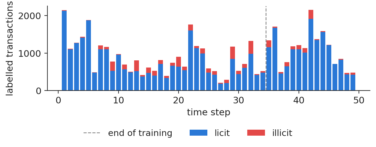
The number of illicit transactions peaks at 342 in step 32; each step has about 4,159 transactions in total. As in Weber et al. (2019), the models are trained on steps 1–34 and tested once on steps 35–49; the steps are never shuffled.

Chart: Illicit transactions over time

Labelled transactions per time step, licit and illicit; the dashed line ends the training period.

Source: Elliptic Bitcoin transaction graph (Weber et al., 2019). Data: Elliptic Bitcoin transaction graph, 49 time steps (about two weeks each).

In practice: a model is judged on the months after its training data, exactly as it will be used.

Degree distribution of the transaction graph

Slide 8 in the PDF

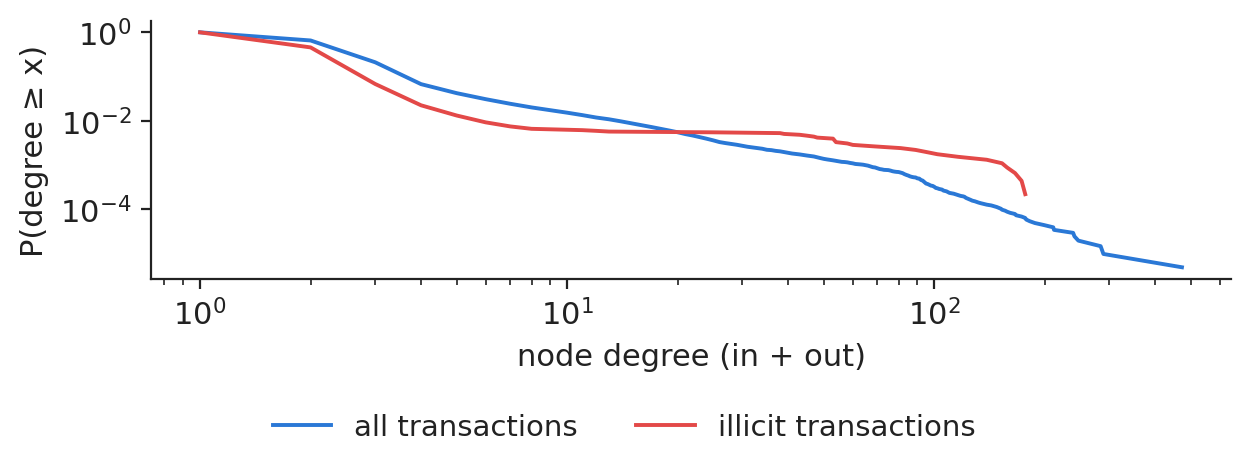
The graph is sparse: the mean degree is 2.30, the median 2, and 34.5 % of the nodes have a single neighbour. The tail is heavy: the largest hub has 473 neighbours. A GNN must not let such hubs drown everyone else, hence the degree normalisation of the next section.

Chart: Degree distribution of the transaction graph

Complementary cumulative distribution of the degree, log-log scale.

Source: Elliptic Bitcoin transaction graph (Weber et al., 2019). Data: Elliptic Bitcoin transaction graph, 49 time steps (about two weeks each).

Homophily of illicit transactions

Slide 9 in the PDF

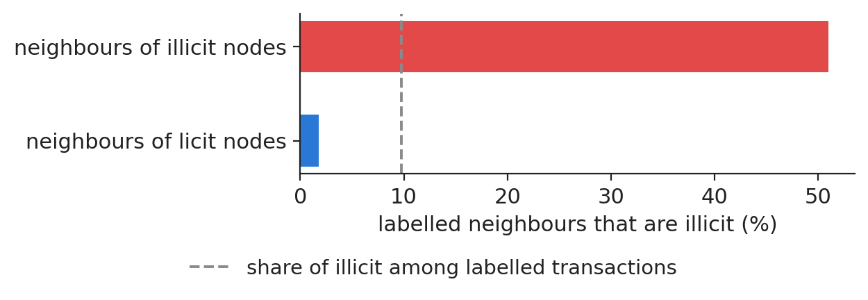
Among the labelled neighbours of an illicit transaction, 51.0 % are illicit; for a licit transaction the share is 1.8 %. Of the labelled edges, 95.4 % join two transactions of the same class, against 82.4 % if labels were assigned at random. This homophily is the reason to look at the neighbours.

Chart: Homophily of illicit transactions

Share of illicit transactions among the labelled neighbours of illicit and of licit transactions.

Source: Elliptic Bitcoin transaction graph (Weber et al., 2019). Data: Elliptic Bitcoin transaction graph, 49 time steps (about two weeks each).

In practice: who you trade with says something about you: homophily is what a GNN exploits.

Section summary

Fraud graphs are sparse, heavy-tailed, labelled in waves and homophilous: neighbours carry information, but time must be respected.

Graphs as matrices

Adjacency, degree and the Laplacian turn a graph into linear algebra.

The adjacency matrix as an algebraic representation of the graph

Slide 11 in the PDF

\(A_{uv}=1\) if \((u,v)\) is an edge and 0 otherwise; \(D=\operatorname{diag}(\sum_vA_{uv})\) is the degree matrix. Adding self-loops and normalising symmetrically gives

\[\tilde A=A+I,\qquad \hat A=\tilde D^{-1/2}\tilde A\,\tilde D^{-1/2},\]
(9.1)

whose entries are \(1/\sqrt{\tilde d_u\tilde d_v}\). The matrix \(A\) has about \(4\cdot10^{10}\) cells but only 234,355 edges, so libraries such as PyTorch Geometric (PyG) store an edge list. Without normalisation, a hub of degree 473 would add 473 messages and explode the scale.

Permutation invariance and equivariance of graph models

Slide 12 in the PDF

For every permutation matrix \(P\), a node-level model must satisfy \(f(P\mathbf X,PAP^\top)=Pf(\mathbf X,A)\) (equivariance) and a graph-level model \(g(P\mathbf X,PAP^\top)=g(\mathbf X,A)\) (invariance). A multilayer perceptron (MLP) on the rows of \(A\) would change with the numbering; a convolutional neural network (CNN) assumes a grid with a fixed number of ordered neighbours, while a transaction has between 1 and hundreds of neighbours in no order.

In practice: ask of any vendor model: does the score change if the input file is sorted differently? It must not.

Smooth signals on a graph: the Laplacian

Slide 13 in the PDF

The Laplacian \(L=D-A\) measures how much a node signal differs between neighbours: \(\mathbf x^\top L\mathbf x=\sum_{(u,v)\in\mathcal E}(x_u-x_v)^2\). Its eigenvectors \(U\) define a graph Fourier transform, \(\hat{\mathbf x}=U^\top\mathbf x\), and a spectral filter is \(U g_\theta(\Lambda)U^\top\mathbf x\). That is costly, but a first-order polynomial in \(L\) leads directly to the normalised adjacency of (9.1) (derivation in Appendix A of the slides). On homophilous fraud graphs the signal is smooth, so averaging over neighbours removes noise, not information.

Three prediction tasks: node, edge and graph level

Slide 14 in the PDF

The same layers serve three questions; only the read-out changes. Node: is this transaction illicit (this lecture)? Edge: is this payment a transfer through a mule account? Graph: is this cluster of accounts a laundering ring, is this interbank network fragile? A sum over node representations makes a graph-level output independent of the numbering.

In practice: define the unit of decision first (a payment, a client, a ring), then the graph task.

Section summary

A GNN works with the normalised adjacency and must be permutation-equivariant; the Laplacian explains why neighbour averages are low-pass filters.

Message passing

Every GNN layer collects messages from the neighbours, aggregates them and updates the node.

A GNN layer: message, aggregation and update functions

Slide 16 in the PDF

A message-passing neural network (MPNN) computes, for each node \(v\) and layer \(l\),

\[\mathbf m_v^{(l)}=\bigoplus_{u\in\mathcal N(v)}\phi^{(l)}\big(\mathbf h_u^{(l)},\mathbf h_v^{(l)},\mathbf e_{uv}\big),\qquad \mathbf h_v^{(l+1)}=\psi^{(l)}\big(\mathbf h_v^{(l)},\mathbf m_v^{(l)}\big),\]
(9.2)

starting from \(\mathbf h_v^{(0)}=\mathbf x_v\), where \(\mathcal N(v)\) are the neighbours, \(\phi\) the message function, \(\bigoplus\) a permutation-invariant aggregator (sum, mean, max), \(\psi\) the update and \(\mathbf e_{uv}\) optional edge features. The weights are shared by all nodes, so the model size does not grow with the graph.

The aggregator and the expressive power of a GNN

Slide 17 in the PDF

Mean and max forget how many neighbours sent a message: the neighbourhoods \(\{a,a\}\) and \(\{a\}\) have the same mean and the same maximum, but different sums. The graph isomorphism network (GIN) uses \(\mathbf h_v^{(l+1)}=\mathrm{MLP}\big((1+\varepsilon)\mathbf h_v^{(l)}+\sum_{u}\mathbf h_u^{(l)}\big)\) and is as discriminative as the Weisfeiler–Leman (WL) test. In fraud, ``one payment from a mixer'' and ``ten payments from mixers'' should not look the same; but sums over hubs need normalisation, which is why the GCN uses (9.1).

In practice: choose the aggregator for the question: counts matter (sum), proportions matter (mean), one red flag matters (max).

Each layer widens the neighbourhood that reaches a node

Slide 18 in the PDF

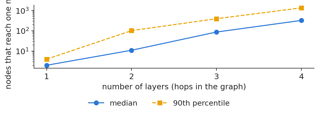
An \(L\)-layer network sees the \(L\)-hop neighbourhood. For 2,000 test transactions the median number of nodes that can influence a node is 2 after one layer, 11 after two and 325 after four; the 90th percentile reaches 1,356 nodes after four layers, because hubs connect distant parts of the graph.

Chart: Each layer widens the neighbourhood that reaches a node

Number of nodes within \(k\) hops of a test transaction, median and 90th percentile.

Source: Elliptic Bitcoin transaction graph (Weber et al., 2019). Data: Elliptic Bitcoin transaction graph, 49 time steps (about two weeks each).

Over-smoothing in deep graph networks

Slide 19 in the PDF

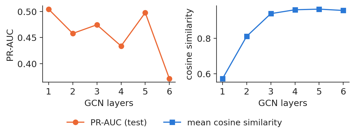
Repeated degree-weighted averaging drives all representations towards a common vector. On Elliptic the test PR-AUC is 0.504 with one GCN layer, 0.458 with two and 0.371 with six; the best depth is 1. Over the same range the mean cosine similarity of node representations rises from 0.57 to 0.96.

Chart: Over-smoothing in deep graph networks

Test PR-AUC and mean cosine similarity of the node representations by number of GCN layers (mean of 2 seeds).

Source: Elliptic Bitcoin transaction graph (Weber et al., 2019). Data: own estimates; training steps 1-34, test time steps 35-49.

In practice: GNNs are shallow by design: two or three layers, then residual links if more is needed.

Section summary

Message passing = message, aggregation, update; depth = hops, and too much depth over-smooths.

GCN, GraphSAGE and GAT

Three choices of message, aggregation and update, from fixed degree weights to learned attention.

GCN: degree-weighted average of the neighbours followed by a linear map

Slide 21 in the PDF

A GCN layer is

\[H^{(l+1)}=\mathrm{ReLU}\big(\hat AH^{(l)}W^{(l)}\big),\]
(9.3)

a linear regression on the normalised average of a node and its neighbours, followed by the rectified linear unit (ReLU). Our GCN has 2 layers of 100 hidden units and dropout 0.2, 26,902 parameters, and is trained on the whole graph at once in about 66 seconds per seed on a laptop processor. The cost per layer is linear in the number of edges.

In practice: a GCN is the graph analogue of a moving average: robust, cheap, and blind to which neighbour matters most.

GraphSAGE: separate node representation and neighbour sampling

Slide 22 in the PDF

GraphSAGE uses separate weights for the node and for the mean of a sample \(\mathcal S(v)\) of its neighbours: \(\mathbf h_v^{(l+1)}=\mathrm{ReLU}\big(W_1\mathbf h_v^{(l)}+W_2\,\mathrm{mean}_{u\in\mathcal S(v)}\mathbf h_u^{(l)}\big)\). The weights do not depend on the graph, so tomorrow's transactions get a score without retraining (inductive learning), and sampling bounds the cost per node. On Elliptic its illicit-class F1 is 0.564 (standard deviation 0.022) and its PR-AUC 0.582.

GAT: learned attention weights over the neighbours

Slide 23 in the PDF

A graph attention layer weights each neighbour by a learned score,

\[\alpha_{vu}=\operatorname{softmax}_u\Big(\mathrm{LeakyReLU}\big(\mathbf a^\top[W\mathbf h_v\,\|\,W\mathbf h_u]\big)\Big),\]
(9.4)

and averages \(W\mathbf h_u\) with these weights, with several heads concatenated. It is the attention of Lecture 7 restricted to the edges of the graph: a transformer is a GAT on the complete graph of the tokens. Our GAT has 4 heads, 27,302 parameters, an illicit F1 of 0.489 and a PR-AUC of 0.496.

In practice: attention weights are a first, not a final, explanation: they show where the model looked, not why.

Training on one big graph: masks, class weights, early stopping

Slide 24 in the PDF

All nodes pass messages, but only the labelled nodes of steps 1–29 enter the weighted cross-entropy, with weights 0.7 for illicit and 0.3 for licit as in Weber et al. (2019). The labelled nodes of steps 30–34 choose the best epoch by PR-AUC (patience 40); the median epoch kept by the GCN is 47. Feature means and standard deviations come from steps 1–34 only. The unknown nodes are not wasted: they carry messages between labelled ones (semi-supervised learning).

Section summary

GCN averages with degree weights, GraphSAGE separates self and neighbours and is inductive, GAT learns the weights.

Case study: illicit Bitcoin transactions

Eight models on the same temporal test, judged like an investigation team would judge them.

Eight models evaluated on a chronological test set

Slide 26 in the PDF

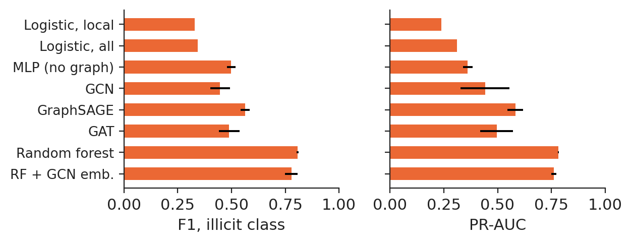
The models are a logistic regression on the 93 local features and on all 165 features; a random forest with 100 trees and 50 features per split, as in Weber et al. (2019); an MLP with the same layers as the GCN but no messages, which isolates the value of the edges; GCN, GraphSAGE and GAT; and a random forest on the features plus the 100 hidden GCN outputs. Precision, recall and F1 of the illicit class are measured at threshold 0.5 on steps 35–49, together with the threshold-free PR-AUC; each network and forest is run with 3 seeds.

Results on Elliptic: the random forest and the contribution of graph layers

Slide 27 in the PDF

The illicit-class F1 is 0.808 for the random forest, 0.778 for the forest with GCN embeddings, 0.447 for the GCN, 0.498 for the MLP and 0.343 for the logistic regression. With the same layers, the edges change the PR-AUC of the network by +8.1 points (GCN against MLP), while its F1 at the 0.5 threshold is lower than the MLP's; GraphSAGE, which keeps the node apart from its neighbours, is the best graph network, with F1 0.564.

Chart: Results on Elliptic: the random forest and the contribution of graph layers

Illicit-class F1 and PR-AUC on test steps 35–49, mean and standard deviation over the seeds.

Source: Elliptic Bitcoin transaction graph (Weber et al., 2019). Data: own estimates; training steps 1-34, test time steps 35-49.

Precision, recall and the cost of training

Slide 28 in the PDF

Precision is the share of alerts that are illicit; recall is the share of illicit transactions found. The random forest has precision 0.914 and recall 0.725; the GCN has precision 0.484 and recall 0.494; the logistic regression, with class weights 0.3 and 0.7, buys a recall of 0.771 with a precision of only 0.220.

In practice: the right model depends on what an error costs: a missed laundering case or an analyst's wasted hour.

Precision-recall curves of the models

Slide 29 in the PDF

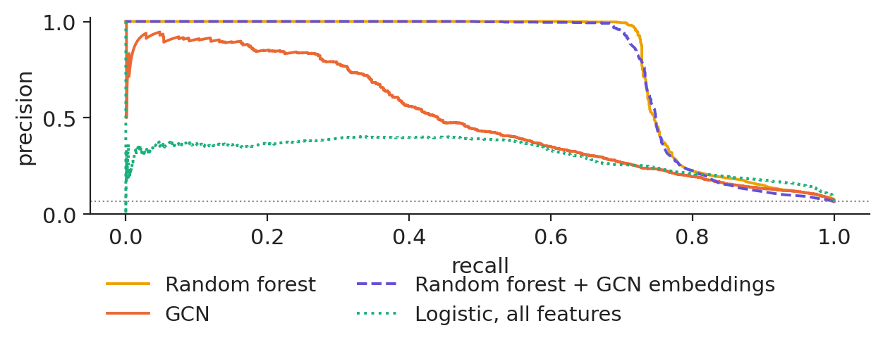
The PR-AUC is 0.782 for the random forest, 0.763 for the forest with GCN embeddings, 0.442 for the GCN and 0.311 for the logistic regression; a random score would give 6.50 %, the share of illicit among the labelled test transactions.

Chart: Precision-recall curves of the models

Precision-recall curves on the test steps (scores averaged over the seeds); the dotted line is the base rate.

Source: Elliptic Bitcoin transaction graph (Weber et al., 2019). Data: own estimates; training steps 1-34, test time steps 35-49.

Bootstrap test of the gap on the test transactions

Slide 30 in the PDF

Resampling the test transactions 1,000 times, with the same draw for both models, gives a PR-AUC difference of 0.285 between the random forest and the GCN, with a 95 % interval of [0.259; 0.313], and a difference of −0.008 between the forest with GCN embeddings and the plain forest, interval [−0.015; −0.002]. An interval that excludes zero supports a real difference on this test period.

In practice: report the interval, not only the winner: a fraud committee decides on ranges, not on the third decimal.

Neighbourhood aggregates in the features and the performance of the random forest

Slide 31 in the PDF

72 of the 165 features are aggregates over the one-hop neighbours (maxima, minima, standard deviations, correlations): one fixed GNN layer computed by Elliptic before release. A logistic regression on the local features alone reaches an F1 of 0.329, against 0.343 with the aggregates. Trees also fit rule-like fraud patterns well. GNNs earn their keep on raw graphs without engineered aggregates, on multi-hop patterns and in inductive scoring; combining both, the forest with GCN representations changes the F1 by −3.0 points.

In practice: before training a GNN, check whether the data provider has already aggregated the neighbourhood for you.

Concept drift after a dark-market shutdown

Slide 32 in the PDF

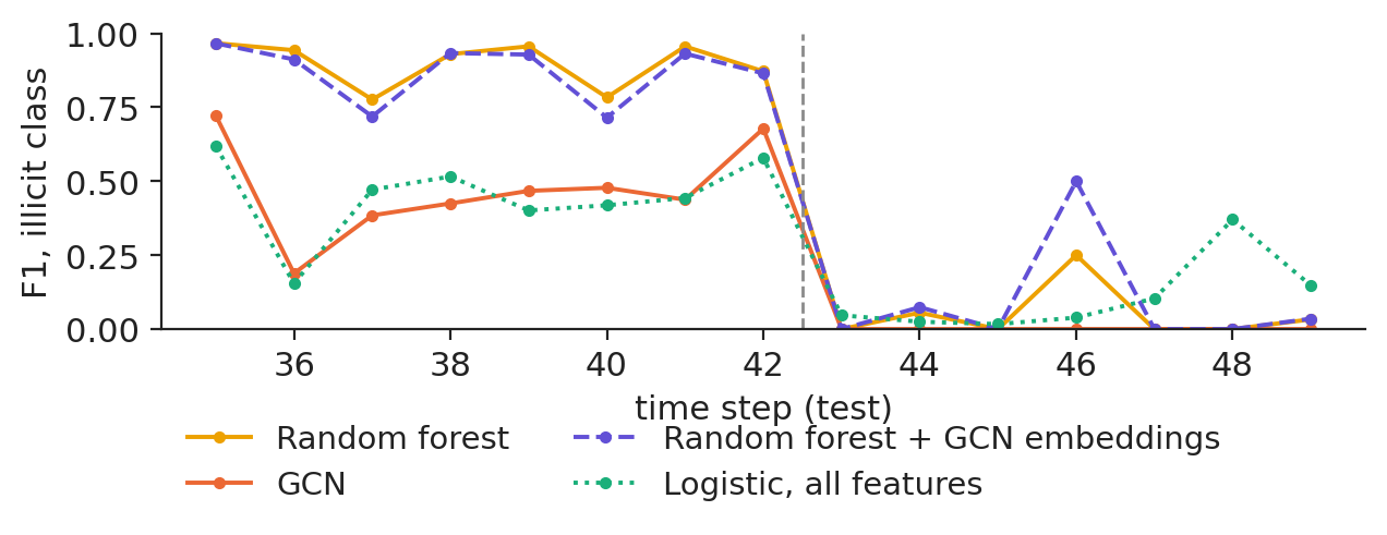
Before step 43 the mean F1 is 0.898 for the random forest and 0.473 for the GCN; from step 43 it is 0.048 and 0.000. After a major dark market closed, illicit flows changed form (Weber et al., 2019), and no model trained on steps 1–34 had seen the new behaviour.

Chart: Concept drift after a dark-market shutdown

Illicit-class F1 per test time step for four models.

Source: Elliptic Bitcoin transaction graph (Weber et al., 2019). Data: own estimates; training steps 1-34, test time steps 35-49.

In practice: monitor F1 per period and retrain on recent labels; a static AML model ages within weeks.

Illicit transactions found among the top 1,000 alerts

Slide 33 in the PDF

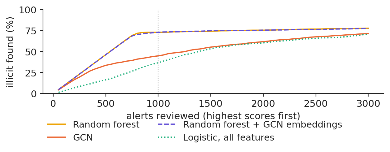
If the team reviews the 1,000 highest scores of the test period, it finds 72.9 % of all illicit transactions with the random forest, 44.8 % with the GCN and 72.9 % with the forest plus GCN representations; the hit rate of those alerts is 78.9 % for the forest and 48.5 % for the GCN, out of 1,083 illicit test transactions.

Chart: Illicit transactions found among the top 1,000 alerts

Share of the illicit test transactions found among the highest scores, by number of alerts reviewed.

Source: Elliptic Bitcoin transaction graph (Weber et al., 2019). Data: own estimates; training steps 1-34, test time steps 35-49.

In practice: size the team from this curve: the alert budget, not the F1, is the constraint in a compliance department.

Illicit transactions cluster in the GCN embedding space

Slide 34 in the PDF

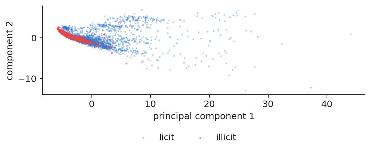
Projecting the 100-dimensional hidden layer of the GCN on its first two principal components (principal component analysis, PCA), which explain 79.2 % of the variance, shows the illicit test transactions gathering in a region of their own. These vectors are the inputs of the forest-plus-GCN model and can feed any other risk model.

Chart: Illicit transactions cluster in the GCN embedding space

Hidden GCN representations of test transactions, first two principal components.

Source: Elliptic Bitcoin transaction graph (Weber et al., 2019). Data: own estimates; training steps 1-34, test time steps 35-49.

Effect of graph features on the explanations

Slide 35 in the PDF

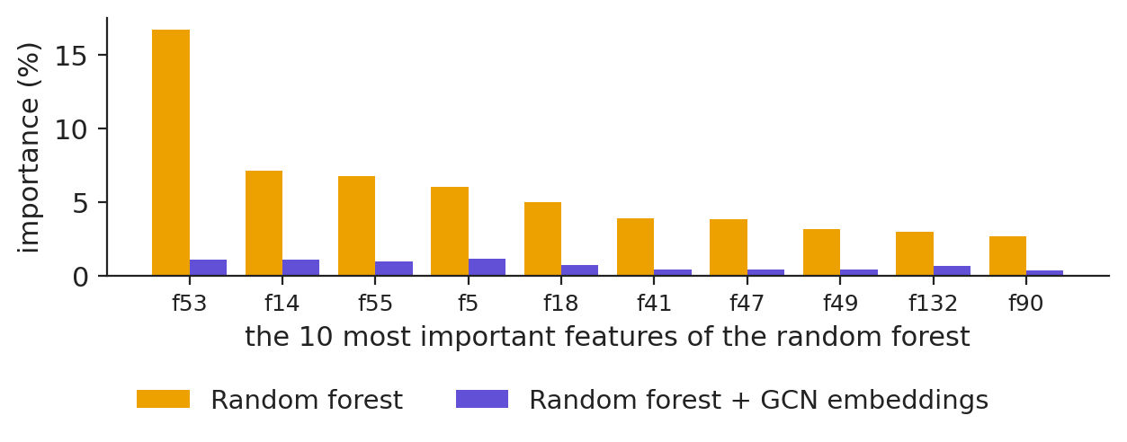
The 10 most important features of the random forest carry 58.2 % of its impurity importance; once the GCN representations are added, the same features keep 7.4 % and the representations take 73.9 %. Across 3 refits, the mean Spearman correlation of the importances is 0.973 for the forest and 0.896 for the forest with GCN representations. Part of the change comes from adding inputs at all, and part from retraining: both must be accounted for before reading a change of model as a change of explanation.

Chart: Effect of graph features on the explanations

Importance of the 10 most important features of the random forest, without and with GCN representations.

Source: Elliptic Bitcoin transaction graph (Weber et al., 2019). Data: own estimates; training steps 1-34, test time steps 35-49.

Section summary

On Elliptic the edges help a network, but a forest on pre-aggregated features leads; drift and alert budgets matter more than the third decimal.

GNNs in production

Graph models in finance fail in specific ways; knowing them is part of the model.

Common errors in applying graph models in finance

Slide 37 in the PDF

Leakage through edges: a test node must not receive messages from the future; in Elliptic 100.0 % of the edges stay inside one time step, so the temporal split is clean. Few labels: only 22.9 % of the nodes are labelled, and labels from past investigations favour the cases already found. Drift: criminals adapt, and temporal GNNs such as EvolveGCN let the weights evolve with time. Explainability: a suspicious-activity report needs a reason a regulator can read; GNNExplainer finds the subgraph and features behind one prediction.

In practice: test a graph model the way it will run: on later periods, with the labels available at that time.

Applications of graph models in finance

Slide 38 in the PDF

Cardholder–merchant graphs link many fraud victims to one compromised terminal; guarantor and supplier networks carry defaults along trade credit; address and transaction graphs reveal mixers and wallet clusters; interbank exposures and tail-dependence networks show who falls if one bank fails; stocks linked by correlation, supply chain or ownership feed return forecasts; power grids and interconnected price zones are graphs by construction.

In practice: whenever the risk of one unit depends on its counterparties, a graph model is worth a try.

Section summary

Respect time, expect few and biased labels, monitor drift and explain decisions: these decide whether a graph model survives in production.

Videos: the intuition behind the mathematics (in English)

Abbreviations

AMLanti-money laundering
ASEBucharest University of Economic Studies
BTCbitcoin (currency unit)
CNNconvolutional neural network
CPUcentral processing unit
GATgraph attention network
GCNgraph convolutional network
GINgraph isomorphism network
GNNgraph neural network
GraphSAGEgraph sample and aggregate
IPEInstitute for Economic Forecasting, Romanian Academy
MLPmultilayer perceptron
MPNNmessage-passing neural network
PCAprincipal component analysis
PR-AUCarea under the precision-recall curve
PyGPyTorch Geometric (library)
ReLUrectified linear unit
SHAPSHapley Additive exPlanations
WLWeisfeiler–Leman graph isomorphism test
XAIexplainable artificial intelligence

References

  • Bishop, C. M. & Bishop, H. (2024). Deep Learning: Foundations and Concepts, ch. 13. Springer. doi:10.1007/978-3-031-45468-4
  • Breiman, L. (2001). Random forests. Machine Learning, 45(1), 5–32. doi:10.1023/A:1010933404324
  • Diaconu, D. & Pele, D. T. (2026). SHAP stability across random and forward-time validation in graph-augmented fraud detection. Submitted to Expert Systems with Applications. Code: github.com/QuantLet/GNN_XAI_Stability
  • Efron, B. & Tibshirani, R. J. (1993). An Introduction to the Bootstrap. Chapman & Hall. doi:10.1201/9780429246593
  • Fey, M. & Lenssen, J. E. (2019). Fast graph representation learning with PyTorch Geometric. ICLR Workshop on Representation Learning on Graphs and Manifolds. arXiv:1903.02428
  • Gilmer, J., Schoenholz, S. S., Riley, P. F., Vinyals, O. & Dahl, G. E. (2017). Neural message passing for quantum chemistry. Proceedings of ICML, PMLR 70, 1263–1272. arXiv:1704.01212
  • Hamilton, W. L., Ying, R. & Leskovec, J. (2017). Inductive representation learning on large graphs. Advances in Neural Information Processing Systems, 30. arXiv:1706.02216
  • Hamilton, W. L. (2020). Graph Representation Learning. Morgan & Claypool. doi:10.2200/S01045ED1V01Y202009AIM046
  • Kipf, T. N. & Welling, M. (2017). Semi-supervised classification with graph convolutional networks. International Conference on Learning Representations. arXiv:1609.02907
  • Li, Q., Han, Z. & Wu, X.-M. (2018). Deeper insights into graph convolutional networks for semi-supervised learning. Proceedings of the AAAI Conference on Artificial Intelligence, 32(1). doi:10.1609/aaai.v32i1.11604
  • Lundberg, S. M. & Lee, S.-I. (2017). A unified approach to interpreting model predictions. Advances in Neural Information Processing Systems, 30. arXiv:1705.07874
  • Pareja, A., Domeniconi, G., Chen, J. et al. (2020). EvolveGCN: Evolving graph convolutional networks for dynamic graphs. Proceedings of the AAAI Conference on Artificial Intelligence, 34(4), 5363–5370. doi:10.1609/aaai.v34i04.5984
  • Toma, F.-M., Dima, D.-M., Grecu, R., Pele, D. T. & Lessmann, S. (2026). Energy Financial Risk Meter: Systemic risk in the EU energy sector. SSRN Working Paper 6985301. doi:10.2139/ssrn.6985301
  • Veličković, P., Cucurull, G., Casanova, A., Romero, A., Liò, P. & Bengio, Y. (2018). Graph attention networks. International Conference on Learning Representations. arXiv:1710.10903
  • Weber, M., Domeniconi, G., Chen, J., Weidele, D. K. I., Bellei, C., Robinson, T. & Leiserson, C. E. (2019). Anti-money laundering in Bitcoin: Experimenting with graph convolutional networks for financial forensics. KDD Workshop on Anomaly Detection in Finance. arXiv:1908.02591
  • Xu, K., Hu, W., Leskovec, J. & Jegelka, S. (2019). How powerful are graph neural networks? International Conference on Learning Representations. arXiv:1810.00826
  • Ying, R., Bourgeois, D., You, J., Zitnik, M. & Leskovec, J. (2019). GNNExplainer: Generating explanations for graph neural networks. Advances in Neural Information Processing Systems, 32. arXiv:1903.03894

Text written for the web version of the lecture; numbers, charts and sources come from the slides and their Quantlets.