

Statistics of Financial Markets

Chapter 14 · Crypto Assets

The slide of the lecture is on the left, the same figure or table on the right, computed in the browser from the same data. The ▶ button moves the parameter step by step; the tables and worked examples are recomputed with it. Abbreviations: BTC (Bitcoin), ETF (exchange-traded fund), IBIT (iShares Bitcoin Trust), USDT (Tether), USDC (USD Coin), DAI (Dai), UST (TerraUSD), SVB (Silicon Valley Bank), FDIC (Federal Deposit Insurance Corporation), ACF (autocorrelation function), VR (variance ratio), HAC (heteroskedasticity- and autocorrelation-consistent standard errors), GARCH (generalised autoregressive conditional heteroskedasticity), GJR (the asymmetric GARCH of Glosten, Jagannathan and Runkle), IGARCH (integrated GARCH), AR(1) (autoregressive process of order 1), CI (confidence interval), HS (historical simulation), VaR (value at risk), ES (expected shortfall), TE (tracking error), bp (basis points), i.i.d. (independent and identically distributed).

Bitcoin and Ethereum in Brief · Crypto as an Asset Class · Tails and Volatility Clustering · Efficiency of the Crypto Market · Correlation with Equities and Gold · Bubbles and Crashes · Spot Bitcoin ETFs · Stablecoins · The Risk of a Crypto Position

Bitcoin and Ethereum in Brief

Bitcoin Price and Supply
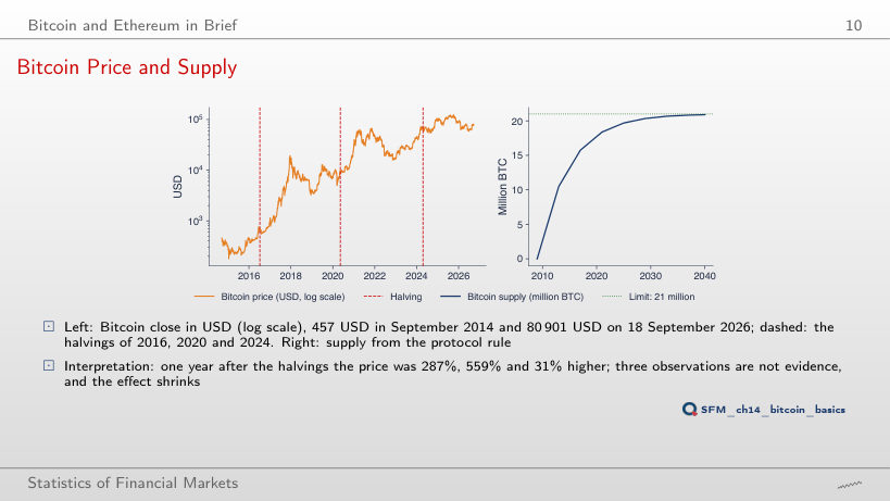
Slide 10: Bitcoin Price and Supply
Slide 10
    Question for the room ▶ shortens the horizon to 180 days (extra run). How much higher was the price 180 days after the April 2024 halving?
    Answer

    By 3.7%, against 31% after one year. For the 2016 and 2020 halvings the 180-day changes are 56% and 72%. The change after a date known in advance depends strongly on the horizon chosen, and three observations allow no conclusion: in an efficient market, an announced cut in supply is already in the price.

    Crypto as an Asset Class

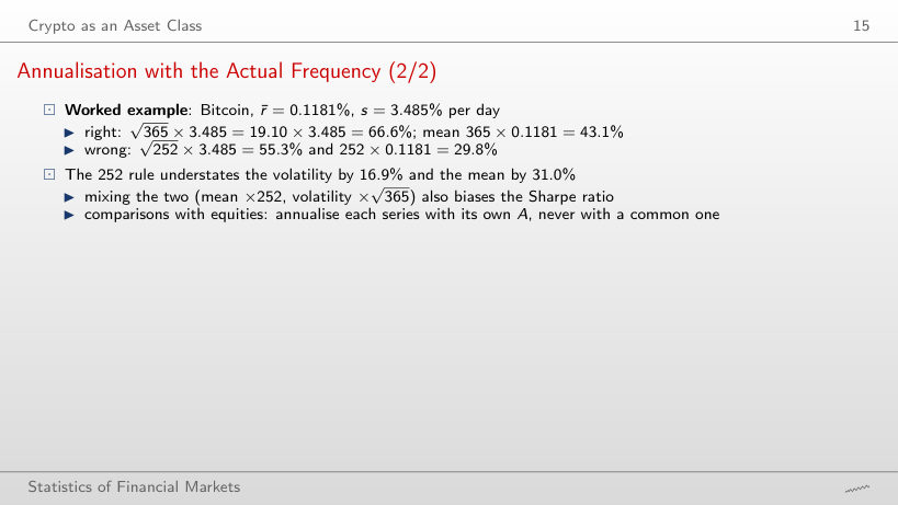
    Annualisation with the Actual Frequency (2/2)
    Slide 15: Annualisation with the Actual Frequency (2/2)
    Slide 15

    Worked example: annualisation with the actual frequency

    \[\text{annual volatility} = \sqrt{A}\,s, \qquad \text{annual mean} = A\,\bar r\]
        Question for the room By how much does the 252 rule understate Bitcoin’s annual volatility, compared with A = 365?
        Answer

        By 16.9% = 1 − √(252/365): 55.3% instead of 66.6%. The mean is understated more, by 31.0% = 1 − 252/365 (29.8% instead of 43.1%), because the mean scales with A and the volatility only with √A.

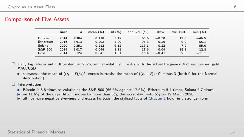
        Comparison of Five Assets
        Slide 16: Comparison of Five Assets
        Slide 16

        Statistics of the daily log returns (the table of the slide)

          Question for the room ▶ starts all series on 1 January 2024 (extra run). How many times as volatile as the S&P 500 is Bitcoin?
          Answer

          3.1 times (47.5% against 15.2%), against 3.8 times on the whole sample; Ethereum 4.5 times, Solana 5.2 times. Bitcoin’s volatility has fallen, but the ratio stays large.

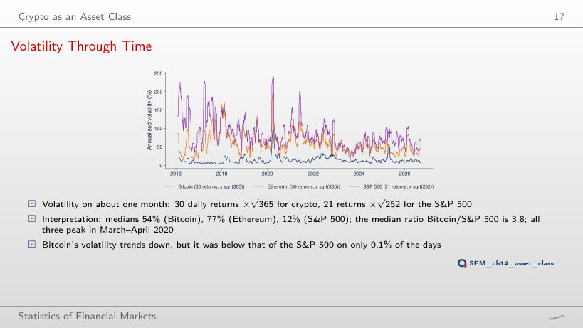
          Volatility Through Time
          Slide 17: Volatility Through Time
          Slide 17
            Question for the room With a 7-day window (▶, extra run), on what share of the days is Bitcoin’s volatility below that of the S&P 500?
            Answer

            On 3.8% of the common days, against 0.11% with the 30-day window. On 7 returns the estimates are much noisier, so the two curves cross more often, although the median ratio stays 3.9.

            Bitcoin Volatility by Day of the Week
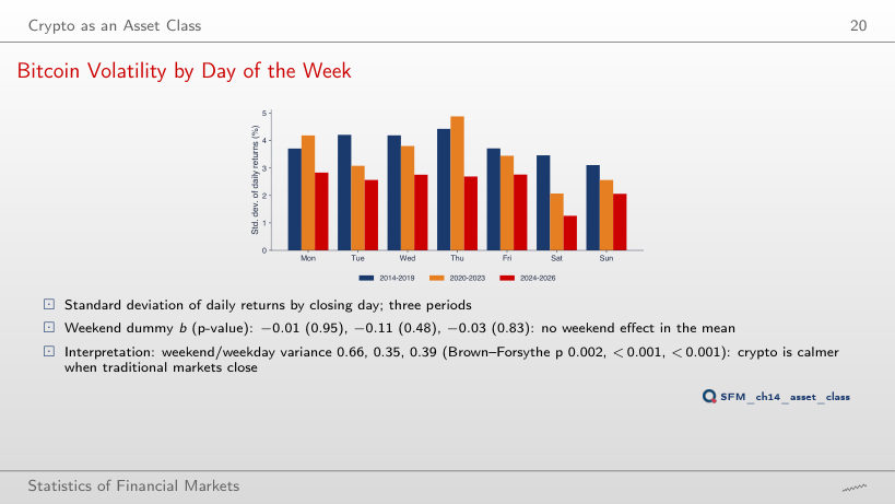
            Slide 20: Bitcoin Volatility by Day of the Week
            Slide 20
              Question for the room ▶ adds one year at a time. In which year is Bitcoin’s ratio of the weekend to the weekday variance lowest?
              Answer

              In 2022: 0.30 (Brown–Forsythe p < 0.001), then 2023 (0.31) and 2024 and 2026 (0.32). Before 2020 the ratio was closer to 1: 0.66 in 2015 and 0.89 in 2016. The weekend mean is not significantly different from the weekday mean in any year.

              Tails and Volatility Clustering

              Heavy Tails: the Hill Estimator (2/2)
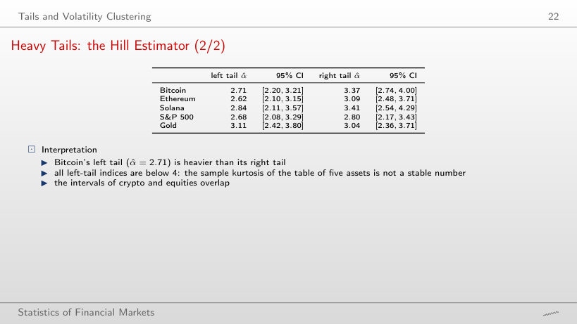
              Slide 22: Heavy Tails: the Hill Estimator (2/2)
              Slide 22

              Hill tail indices (the table of the slide)

                Question for the room With k = 10% of n (▶, extra run), what happens to Bitcoin’s left-tail α̂?
                Answer

                It falls to 1.83 (k = 438), from 2.71 with k = 2.5%; with k = 1% it rises to 3.83. A large k takes in observations from the centre of the distribution, where the power law does not hold, and the estimate falls; k = 2.5% of n is a choice, not a result.

                Reading the ACF and the Ljung–Box Test
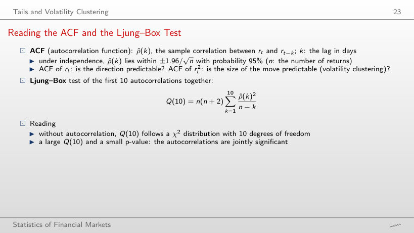
                Slide 23: Reading the ACF and the Ljung–Box Test
                Slide 23

                The Ljung–Box Q(m) of rₜ and rₜ², with p-values

                Worked example: the Ljung–Box statistic

                \[Q(m) = n(n + 2)\sum_{k=1}^{m}\frac{\hat\rho(k)^2}{n - k} \sim \chi^2(m)\]
                    Question for the room For Bitcoin’s returns rₜ, from which m is Q(m) significant at 5% for the first time (▶, m = 1 … 30)?
                    Answer

                    From m = 10: Q(10) = 20.2 against the critical value 18.3. At m = 12 it is not (20.6 < 21.0), nor at m = 30 (43.5 < 43.8). The autocorrelations of the returns are small, so the verdict depends on the number of lags; for rₜ² Q(m) exceeds the critical value at every m.

                    Volatility Clustering in Bitcoin
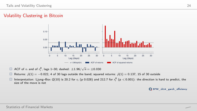
                    Slide 24: Volatility Clustering in Bitcoin
                    Slide 24
                      Question for the room ▶ goes through the five series. Which has the largest first-order autocorrelation of the squared returns?
                      Answer

                      The S&P 500: ρ̂(1) = 0.451, then Solana 0.247, Ethereum 0.175, Bitcoin 0.137 and gold 0.090. Volatility clustering is not about the level of volatility: equities have a lower volatility, but one that is more persistent from one day to the next.

                      GARCH(1,1)-t for Crypto and Traditional Assets (2/2)
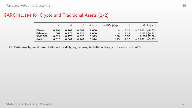
                      Slide 26: GARCH(1,1)-t for Crypto and Traditional Assets (2/2)
                      Slide 26

                      GARCH(1,1)-t and GJR estimates (the table of the slide) and the share of a shock left

                      Worked example: the half-life of a shock

                      \[h_{1/2} = \frac{\ln 0.5}{\ln(\alpha + \beta)}, \qquad \text{share left after } h \text{ days} = (\alpha + \beta)^h\]
                          Question for the room What share of a volatility shock is still in the S&P 500 variance after 200 days?
                          Answer

                          About 25%: 0.9931²⁰⁰ = 0.251, two half-lives of 100 days. For gold 29% is left, for Bitcoin practically 100%, because α̂ + β̂ = 1.

                          Conditional Volatility: Bitcoin and the S&P 500
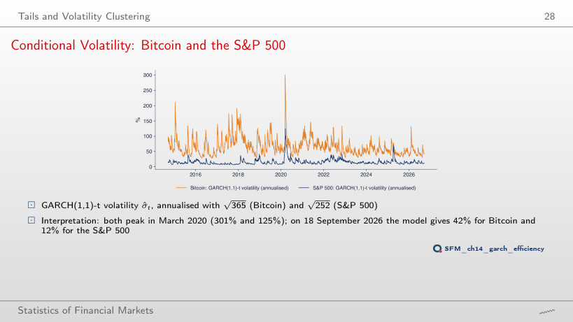
                          Slide 28: Conditional Volatility: Bitcoin and the S&P 500
                          Slide 28
                            Question for the room ▶ extends the forecast to 365 days. What volatility does the model give for Bitcoin one year ahead?
                            Answer

                            About 169%, from 54% for the next day. With α̂ + β̂ = 1 the forecast variance grows by ω̂ = 0.194 every day, with no return to a long-run level. For the S&P 500 the forecast rises from 11.5% to 28.4%, towards the long-run level of 29.4%.

                            Efficiency of the Crypto Market

                            Variance-Ratio Tests on the Whole Sample
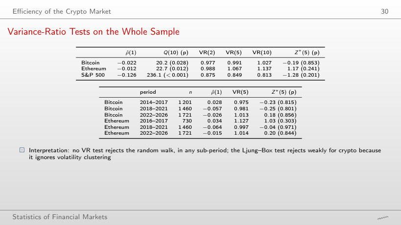
                            Slide 30: Variance-Ratio Tests on the Whole Sample
                            Slide 30

                            Whole sample (the first table of the slide)

                            Sub-periods (the second table of the slide)

                              Question for the room With q = 2 (▶, extra run), does any whole-sample Z* reject the random walk at 5%?
                              Answer

                              Yes, for the S&P 500: Z*(2) = −2.30 (p 0.022), because VR(2) = 0.875 ≈ 1 + ρ̂(1) reflects the daily mean reversion of the index. Bitcoin (−0.88) and Ethereum (−0.43) do not reject. The rejection comes from the market seen as the most efficient, not from crypto.

                              Efficiency Through Time
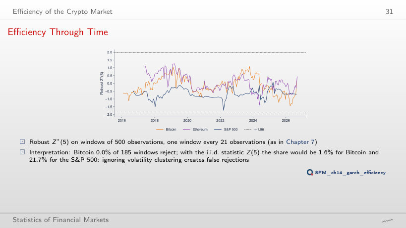
                              Slide 31: Efficiency Through Time
                              Slide 31
                                Question for the room With windows of 1,000 observations (▶, extra run), what share of the S&P 500 windows reject with the i.i.d. Z(5)?
                                Answer

                                About 50% (50.5%), against 21.7% with windows of 500, and still 0% with the robust Z*. A longer window gives more power to a wrong test: ignoring volatility clustering creates false rejections.

                                Correlation with Equities and Gold

                                Measuring Correlation Across Calendars
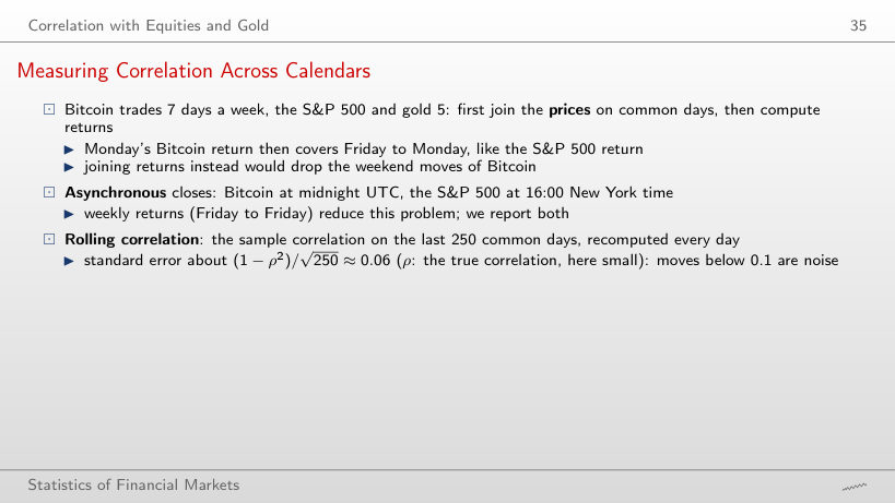
                                Slide 35: Measuring Correlation Across Calendars
                                Slide 35

                                Worked example: the correlation on one rolling window

                                \[\hat\rho = \frac{\widehat{\mathrm{Cov}}(r^A, r^B)}{s_A\,s_B}, \qquad \mathrm{SE}(\hat\rho) \approx \frac{1 - \hat\rho^2}{\sqrt{w}}\]
                                    Question for the room With a 60-day window (▶, extra run), is the highest Bitcoin–S&P 500 rolling correlation above or below 0.57?
                                    Answer

                                    Above: 0.67, on 25 October 2024. The standard error near ρ = 0 is 1/√60 = 0.13, against 0.063 with 250 days: short windows give more extreme values.

                                    Rolling Correlation with Equities and Gold
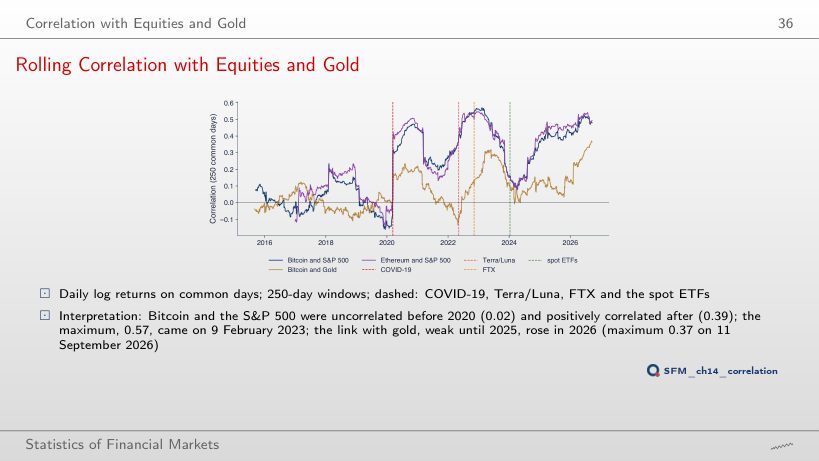
                                    Slide 36: Rolling Correlation with Equities and Gold
                                    Slide 36
                                      Question for the room With a 500-day window (▶, extra run), what is the maximum of the Bitcoin–gold rolling correlation?
                                      Answer

                                      About 0.25, on 18 September 2026, against 0.37 on 11 September 2026 with 250 days. The long window mixes 2026 with 2024–2025, when the correlation was 0.12, so the rise of 2026 is diluted.

                                      Correlation Year by Year
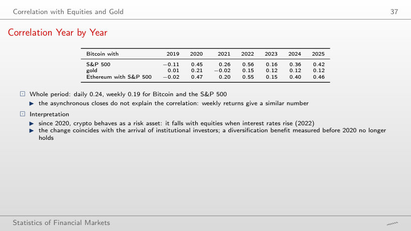
                                      Slide 37: Correlation Year by Year
                                      Slide 37

                                      Correlation year by year (the slide shows 2019–2025)

                                        Question for the room With weekly returns (extra run), is the 2022 correlation of Bitcoin and the S&P 500 higher or lower than with daily returns?
                                        Answer

                                        Lower: 0.43 against 0.56; over the whole period 0.19 against 0.24. Asynchronous closes would lower the daily correlation, not the weekly one; one year has only about 50 weekly returns, so the estimate is noisier.

                                        Three Crisis Episodes
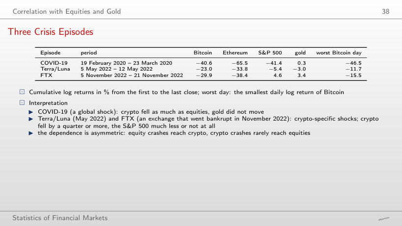
                                        Slide 38: Three Crisis Episodes
                                        Slide 38

                                        Cumulative log returns (%), the table of the slide

                                          Question for the room During the FTX episode (5–21 November 2022), what did the S&P 500 do?
                                          Answer

                                          It rose by 4.6%, and gold by 3.4%, while Bitcoin lost 29.9% and Ethereum 38.4%. A shock specific to crypto did not reach equities.

                                          Bitcoin as a Hedge or a Safe Haven
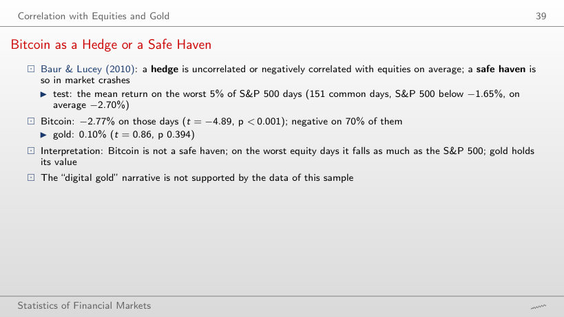
                                          Slide 39: Bitcoin as a Hedge or a Safe Haven
                                          Slide 39

                                          Worked example: the safe-haven test

                                          \[t = \frac{\bar r_{\mathrm{bad}}}{s_{\mathrm{bad}}/\sqrt{n_{\mathrm{bad}}}} \sim t(n_{\mathrm{bad}} - 1)\]
                                              Question for the room On the worst 1% of S&P 500 days (▶, extra run), what is gold’s mean return?
                                              Answer

                                              −0.39% (t = −1.27, p 0.215), not significantly different from zero on those 31 days, while Bitcoin has −6.30% (t = −3.23, p 0.003). Gold holds its value, without rising on the hardest days.

                                              Bubbles and Crashes

                                              Drawdown
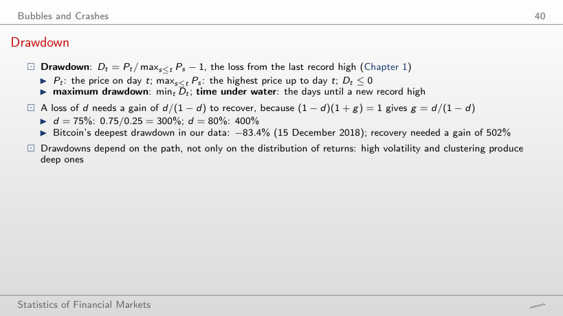
                                              Slide 40: Drawdown
                                              Slide 40

                                              Worked example: the maximum drawdown and the gain needed

                                              \[D_t = \frac{P_t}{\max_{s \le t} P_s} - 1, \qquad (1 - d)(1 + g) = 1 \;\Rightarrow\; g = \frac{d}{1 - d}\]
                                                  Question for the room Ethereum’s maximum drawdown is −94.0%. What gain does it need to recover?
                                                  Answer

                                                  1,556% = 0.940/0.060: from 6.0% of its record value it has to rise about 16.6 times. Ethereum was back at its record on 2 February 2021.

                                                  Drawdowns of Bitcoin, Ethereum and the S&P 500
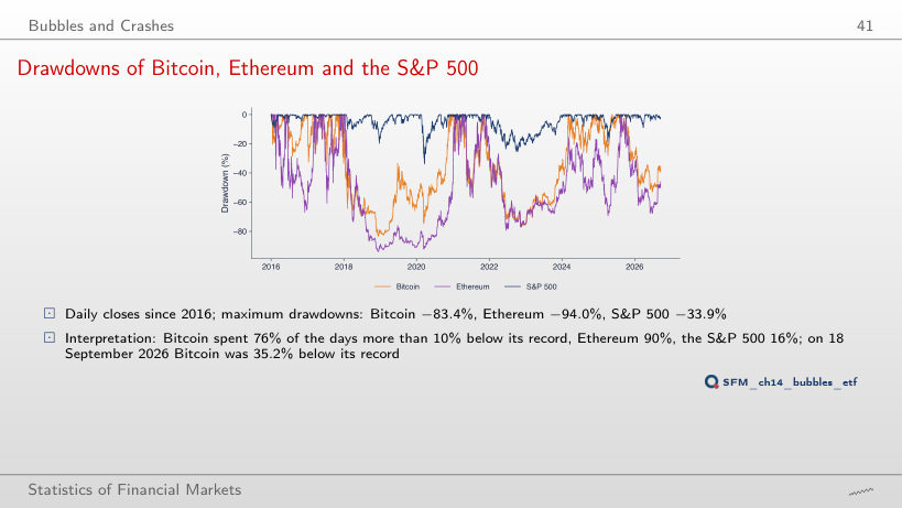
                                                  Slide 41: Drawdowns of Bitcoin, Ethereum and the S&P 500
                                                  Slide 41
                                                    Question for the room ▶ starts the sample in 2022 (extra run). What is Bitcoin’s maximum drawdown?
                                                    Answer

                                                    −66.9%, against −83.4% since 2016. The drawdown is measured from the highest price in the sample, and the peak of November 2021 is no longer in it. Ethereum −74.1%, S&P 500 −25.4%.

                                                    Bitcoin's Large Drawdowns
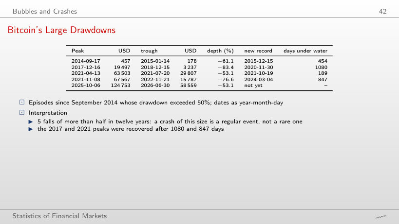
                                                    Slide 42: Bitcoin's Large Drawdowns
                                                    Slide 42

                                                    Bitcoin episodes since September 2014 (the table of the slide)

                                                      Question for the room With a threshold of 30% (▶, extra run), how many Bitcoin episodes are there since September 2014?
                                                      Answer

                                                      Eight: three falls of 2017 (−32.6%, −34.8% and −35.5%), recovered within months, join the five of the slide.

                                                      Spot Bitcoin ETFs

                                                      Volatility and the Weekend Share Around the ETFs
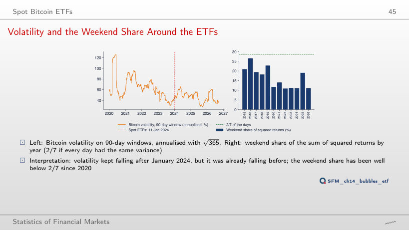
                                                      Slide 45: Volatility and the Weekend Share Around the ETFs
                                                      Slide 45
                                                        Question for the room In which year since 2020 was the weekend share of Bitcoin’s squared returns highest?
                                                        Answer

                                                        In 2025: 19.0%, against 10.9–14.0% in the other years; still below 2/7 = 28.6%, the value for an equal variance on every day.

                                                        Bitcoin before and after the Spot ETFs
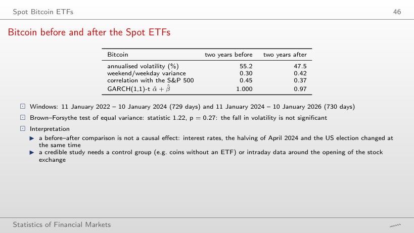
                                                        Slide 46: Bitcoin before and after the Spot ETFs
                                                        Slide 46

                                                        Bitcoin before and after 11 January 2024 (the table of the slide)

                                                          Question for the room With windows of one year (▶, extra run), does the Brown–Forsythe test find a significant change in volatility?
                                                          Answer

                                                          Yes (p 0.001), but volatility rose, from 44.4% to 52.9%. With 2.5 years it is also significant (p 0.008), in the opposite direction (57.2% to 48.0%), and with two years it is not (p 0.27). The result depends on the window, so the before–after comparison does not measure a causal effect of the ETFs.

                                                          Tracking Error of a Spot Bitcoin ETF
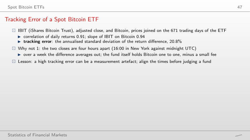
                                                          Slide 47: Tracking Error of a Spot Bitcoin ETF
                                                          Slide 47

                                                          Worked example: tracking error

                                                          \[\mathrm{TE} = \sqrt{252/k}\;\mathrm{sd}\big(r^{\mathrm{IBIT}}_t - r^{\mathrm{BTC}}_t\big)\]
                                                              Question for the room With 5-day returns (▶, extra run), what is IBIT’s tracking error?
                                                              Answer

                                                              8.9% a year, with a correlation of 0.98, against 20.8% for daily returns. The gap between the New York close and the midnight UTC close averages out within days.

                                                              Stablecoins

                                                              Supply of Stablecoins
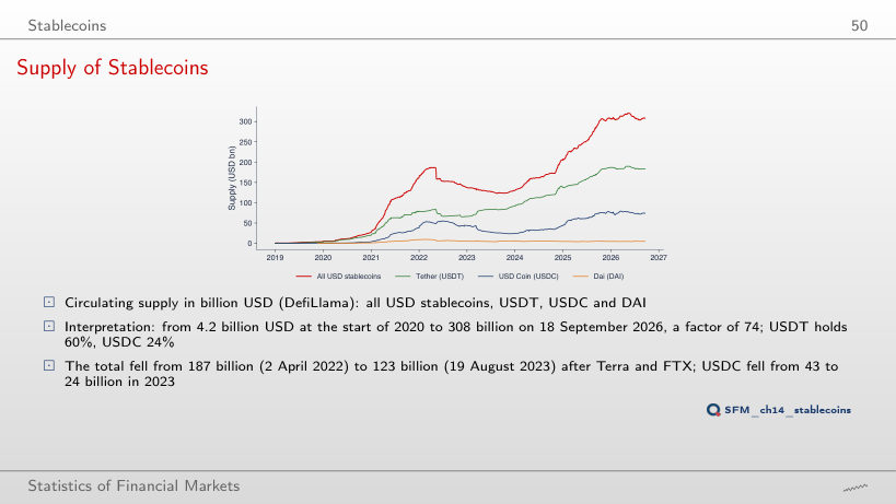
                                                              Slide 50: Supply of Stablecoins
                                                              Slide 50
                                                                Question for the room By how much did the total stablecoin supply fall between 2 April 2022 (187 billion USD) and 19 August 2023 (123 billion)?
                                                                Answer

                                                                By 34.5% = 1 − 122.7/187.4. On the slides the total on 18 September 2026 is 308 billion USD; the download of 4 November 2026 gives 303 billion for the same date, because DefiLlama revises its history.

                                                                Peg Deviation in Basis Points
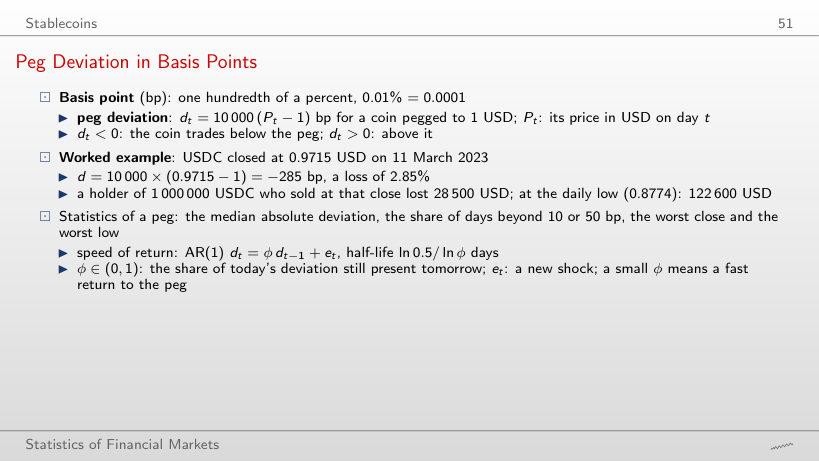
                                                                Slide 51: Peg Deviation in Basis Points
                                                                Slide 51

                                                                Worked example: the peg deviation and the loss

                                                                \[d_t = 10\,000\,(P_t - 1)\ \text{bp}, \qquad \text{loss} = W\,(1 - P_t)\]
                                                                    Question for the room DAI’s low on 11 March 2023 was 0.8970 USD. What is its peg deviation?
                                                                    Answer

                                                                    −1,030 bp = 10,000 × (0.8970 − 1), that is −10.3%. The USDC low on the same day was −1,226 bp.

                                                                    Peg Deviations of USDT, USDC and DAI
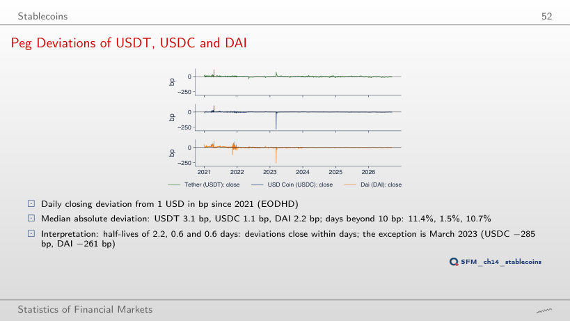
                                                                    Slide 52: Peg Deviations of USDT, USDC and DAI
                                                                    Slide 52

                                                                    Peg statistics since 2021 (the numbers of the slide)

                                                                      Question for the room With a threshold of 50 bp (▶), on what share of the days does DAI’s close deviate by more?
                                                                      Answer

                                                                      On 0.57% of the days (12 of 2,087), against 0.14% for USDT and for USDC; at the 10 bp threshold the shares are 10.7%, 11.4% and 1.5%.

                                                                      The USDC Depeg, Day by Day
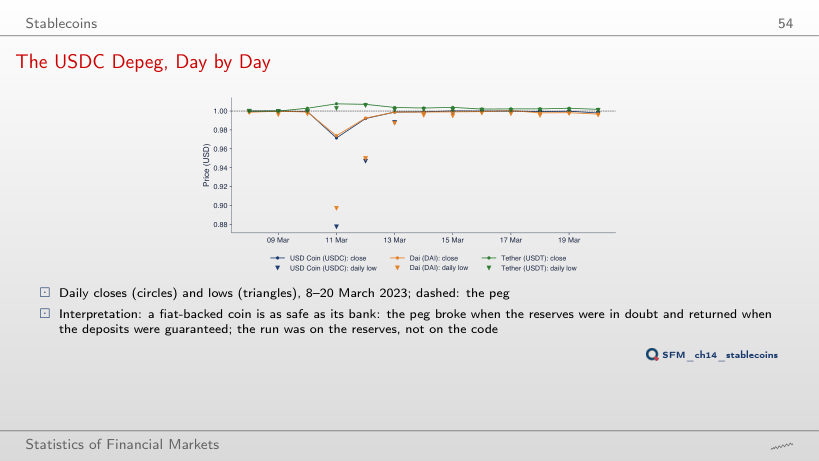
                                                                      Slide 54: The USDC Depeg, Day by Day
                                                                      Slide 54
                                                                        Question for the room Where did USDC close on 13 March 2023?
                                                                        Answer

                                                                        At 0.9989 USD, that is −11 bp, back near the peg after the guarantee of the SVB deposits on the evening of 12 March (U.S. Treasury, Federal Reserve & FDIC, 2023). On 11 March the close had been 0.9715 (−285 bp). USDT closed at +39 bp on 13 March.

                                                                        The Collapse of UST, May 2022
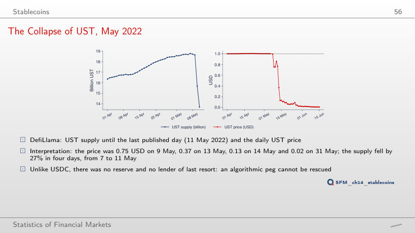
                                                                        Slide 56: The Collapse of UST, May 2022
                                                                        Slide 56
                                                                          Question for the room By how much had the UST supply fallen between its peak on 7 May 2022 and the last published day, 11 May?
                                                                          Answer

                                                                          By 27%, from 18.8 to 13.7 billion UST, in four days. The price fell further: 0.75 USD on 9 May, 0.37 on 13 May and 0.02 on 31 May.

                                                                          The Risk of a Crypto Position

                                                                          VaR 1% and ES 2.5% in Dollars
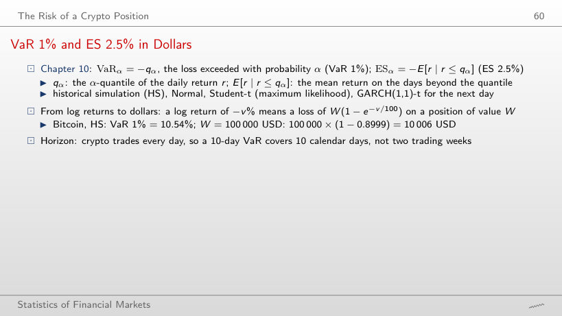
                                                                          Slide 60: VaR 1% and ES 2.5% in Dollars
                                                                          Slide 60

                                                                          Worked example: from the log return to dollars

                                                                          \[\text{loss} = W\,\big(1 - e^{-v/100}\big)\]
                                                                              Question for the room The S&P 500 HS VaR 1% is a log return of −3.256%. What is it for a position of 1,000,000 USD?
                                                                              Answer

                                                                              32,037 USD = 1,000,000 × (1 − e^(−0.03256)). Read as a simple return, the same number would give 32,562 USD.

                                                                              VaR 1% and ES 2.5% under Four Methods
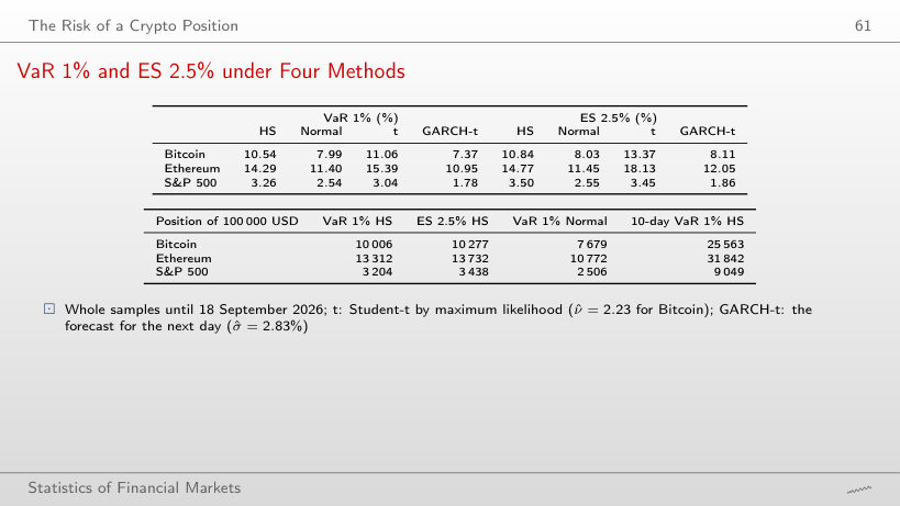
                                                                              Slide 61: VaR 1% and ES 2.5% under Four Methods
                                                                              Slide 61

                                                                              VaR and ES in percent (the first table of the slide)

                                                                              In USD, for a position of 100,000 USD (the second table of the slide)

                                                                                Question for the room At α = 5% (▶, extra run), is Bitcoin’s Normal VaR still below the historical one?
                                                                                Answer

                                                                                No: 5.62% against 5.33% historical, 5% above. Bitcoin’s distribution has heavy tails and a more peaked centre than the Normal distribution: at 1% the Normal distribution understates the loss (7.99% against 10.54%), at 5% it overstates it.

                                                                                Interpretation of the Risk Numbers
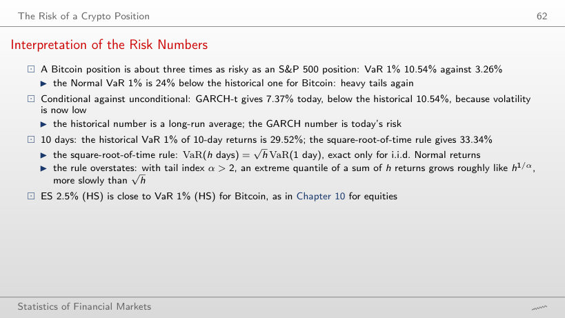
                                                                                Slide 62: Interpretation of the Risk Numbers
                                                                                Slide 62

                                                                                Worked example: the square-root-of-time rule

                                                                                \[\mathrm{VaR}(h\ \text{days}) \overset{?}{=} \sqrt{h}\,\mathrm{VaR}(1\ \text{day})\]
                                                                                    Question for the room For Bitcoin and h = 30 days (▶), does the square-root-of-time rule give more or less than the historical 30-day VaR 1%?
                                                                                    Answer

                                                                                    More: 57.7% against 48.2%, 20% above. With a tail index between 2 and 4, the extreme quantiles of sums grow more slowly than √h.

                                                                                    Backtesting: the Kupiec Test
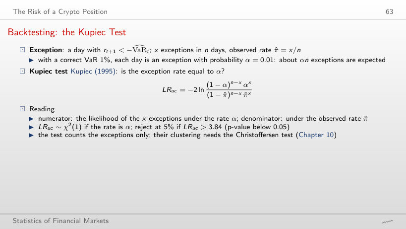
                                                                                    Slide 63: Backtesting: the Kupiec Test
                                                                                    Slide 63

                                                                                    Worked example: the Kupiec test

                                                                                    \[LR_{uc} = -2\ln\frac{(1 - \alpha)^{n - x}\,\alpha^{x}}{(1 - \hat\pi)^{n - x}\,\hat\pi^{x}}, \qquad \hat\pi = \frac{x}{n}\]
                                                                                        Question for the room With n = 3,183 days and α = 1%, which numbers of exceptions does the Kupiec test accept at 5%?
                                                                                        Answer

                                                                                        From 22 to 43. HS (29) and GARCH-t (41) are inside; 41 is near the edge (LR_uc = 2.45, p 0.12). The test also rejects too few exceptions, not only too many.

                                                                                        Backtesting Bitcoin VaR 1%
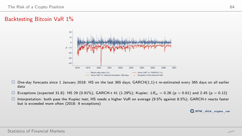
                                                                                        Slide 64: Backtesting Bitcoin VaR 1%
                                                                                        Slide 64
                                                                                          Question for the room With an HS window of 1,000 days (▶, extra run), what does the Kupiec test say?
                                                                                          Answer

                                                                                          It rejects, for too few exceptions: 21 (0.66%), p 0.04. The long window keeps the losses of 2018–2022 and gives a mean VaR of 10.1%, too large for the calmer years.

                                                                                          Course data in data/market (up to 18 September 2026): daily closes of Bitcoin, Ethereum, Solana, the S&P 500, gold (XAU/USD) and the IBIT ETF; daily closes and lows of USDT, USDC and DAI since 2021. The stablecoin supply and the TerraUSD series come from DefiLlama, downloaded with the chapter’s function on 4 November 2026 and cut at 18 September 2026; where the download differs from the values on the slides, the page shows both. The GARCH(1,1)-t and GJR estimates, the conditional volatilities, the Student-t fits and the GARCH-t forecasts of the backtest come from the code of the chapter (Quantlets/Ch_14). From the prices the browser recomputes the returns, the descriptive statistics, the Hill indices, the ACF and the Ljung–Box test, the variance ratios, the correlations, the drawdowns, the weekend and safe-haven tests, the peg deviations, VaR, ES and the Kupiec test. Other windows, thresholds, horizons, periods and levels α are extra runs of the same code; the GARCH persistence on ETF windows of 1, 1.5 and 2.5 years is an extra estimation with the chapter’s code, and the multi-day GARCH forecasts and the share of a shock left are extra computations from the estimates on the slide.