

Statistics of Financial Markets

Chapter 3 · α-Stable Distributions

The slide of the lecture is on the left, the same figure on the right, computed in the browser from the same data. The ▶ button moves the parameter step by step.

Stability under Summation · The Generalised Central Limit Theorem · Parameters and the Characteristic Function · Tails and Moments · Simulation · Estimation · Fitting Real Returns · Critique of the Stable Model: Finite or Infinite Variance

Stability under Summation

Stability in a Simulation
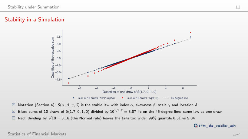
Slide 11: Stability in a Simulation
Slide 11
    Question for the room On the slide, the sum of 10 draws from S(1.7, 0, 1, 0) divided by √10 has a 99% quantile of 6.31, against 5.04 for a single draw. What does this quantile become if we add 50 draws and still divide by √n?
    Answer

    About 7.27. Divided by 501/1.7 = 9.98, the same sum has a 99% quantile of 5.15, the law of a single draw. The √n rule understates the scale of the sum by the factor n1/α − 1/2, which grows with n: 100.088 = 1.23 and 500.088 = 1.41. With infinite variance, more terms do not bring the sum closer to the rule of the Normal distribution.

    Consequences: Horizons and Diversification
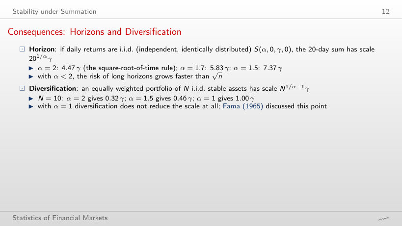
    Slide 12: Consequences: Horizons and Diversification
    Slide 12

    Scale factor of the n-day sum and of the portfolio of N assets (γ = 1)

    Worked example: the scale of n-day risk, with the fitted α̂ and γ̂

    \[X_1 + \dots + X_n \overset{d}{=} n^{1/\alpha}X + d_n, \qquad \gamma_n = n^{1/\alpha}\gamma, \qquad \frac{\gamma_n}{\sqrt{n}\,\gamma} = n^{1/\alpha - 1/2}, \qquad \gamma_{N} = N^{1/\alpha - 1}\gamma\]
        Question for the room On the slide, with α = 1.5 the scale of the 20-day sum is 7.37γ, 1.65 times the factor √20 = 4.47. The ▶ button moves the horizon n up to 250 days. How many times larger is the scale for α = 1.5 than the one given by the square-root-of-time rule at n = 250?
        Answer

        2.51 times: 2501/1.5 = 39.69, against √250 = 15.81. The ratio is n1/α − 1/2 = 2501/6, so it grows with the horizon. With α̂ = 1.540 fitted to the S&P 500, the ratio is 1.56 at 20 days and 2.28 at 250 days. For an equally weighted portfolio of N = 10 assets, the scale falls to 0.46γ for α = 1.5, against 0.32γ for the Normal distribution.

        The Generalised Central Limit Theorem

        The GCLT in a Simulation
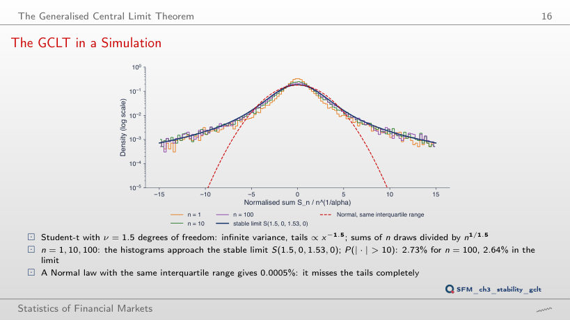
        Slide 16: The GCLT in a Simulation
        Slide 16
          Question for the room At the threshold 10, the Normal distribution with the same interquartile range as the stable limit gives P(|·| > 10) = 0.0005%, against 2.64% for the limit. What probability does the same Normal distribution give at the threshold 3?
          Answer

          17.2%, close to 19.2% for the sums with n = 100 and to 21.7% for the stable limit. The same interquartile range makes the bodies of the two laws similar; the difference is far in the tails: at the threshold 10, 0.0005% against 2.73% in the simulation. The ▶ button shows how the ratio grows with the threshold.

          Parameters and the Characteristic Function

          The Effect of α
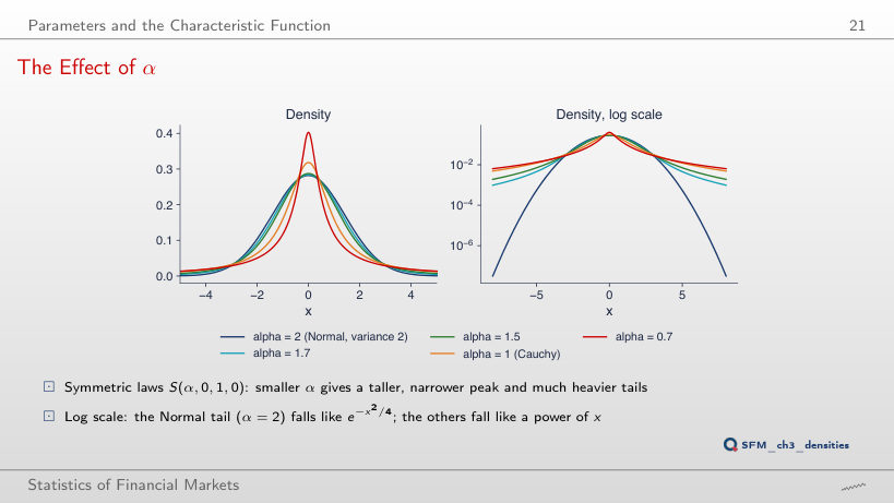
          Slide 21: The Effect of α
          Slide 21
            Question for the room From α = 2 to α = 1.5, what changes more: the density at x = 0 or the density at x = 5?
            Answer

            The density at x = 5. f(0) rises from 0.2821 to 0.2874, by 1.9%, and f(5) rises from 0.000545 to 0.00711, 13 times. On the linear scale the curves look close; the log scale shows that α changes mainly the tails. P(|X| > 5) is 0.041% for α = 2 and 4.14% for α = 1.5.

            The Effect of β and γ
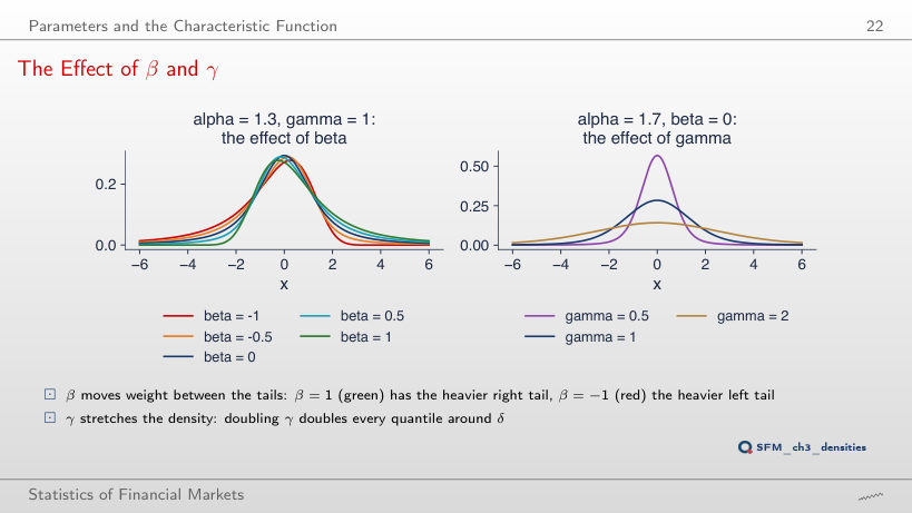
            Slide 22: The Effect of β and γ
            Slide 22
              Question for the room For α = 1.3 and β = 0.5, how many times more likely is a value above 10 than a value below −10?
              Answer

              About 3 times: the ratio is 3.29 at the threshold 10 and tends to (1 + β)/(1 − β) = 1.5/0.5 = 3, from the tail formula P(X > x) ∼ cα(1 + β)x−α and P(X < −x) ∼ cα(1 − β)x−α. At the threshold 3 the probabilities are 10.8% and 3.37%. With β = 1, the left tail falls much faster than x−α.

              S1 vs S0 near α = 1
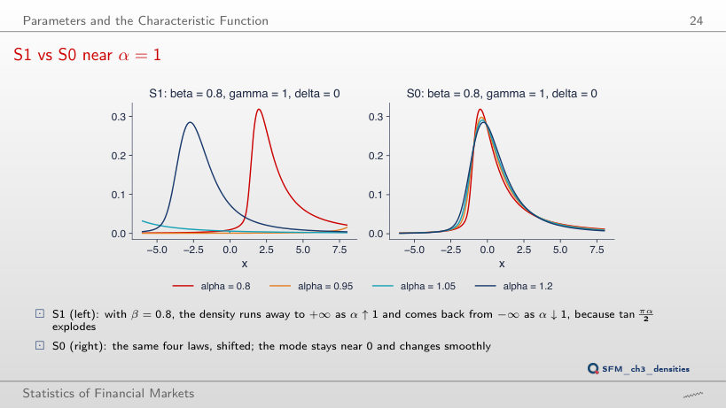
              Slide 24: S1 vs S0 near α = 1
              Slide 24
                Question for the room The ▶ button moves α from 0.80 to 1.20, with β = 0.8. Where is the mode of the density in the S1 parameterisation for α = 0.99?
                Answer

                At about 50.5, far outside the chart. The shift between the two parameterisations is β tan(πα/2) = 0.8 × 63.66 = 50.93, and the mode in S0 is −0.38. At α = 1.01 the tangent changes sign and the mode in S1 moves to about −51. In S0 the mode stays between −0.48 and −0.26 over the whole range.

                Normal, Cauchy and Lévy
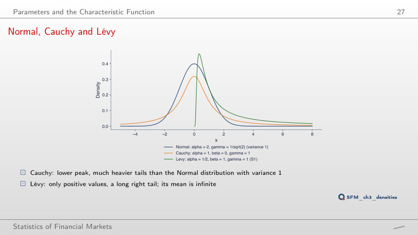
                Slide 27: Normal, Cauchy and Lévy
                Slide 27
                  Question for the room For the threshold x = 20, which of the three laws has the largest probability P(X > x)?
                  Answer

                  The Lévy law: 17.7%, against 1.59% for the Cauchy and about 3 × 10−87% for the Normal distribution. The Lévy tail falls as x−1/2 (α = 1/2), the Cauchy tail as x−1. For x = 3 the probabilities are 43.6% (Lévy), 10.2% (Cauchy) and 0.13% (Normal distribution).

                  Worked Example: S1 vs S0 at t = 1
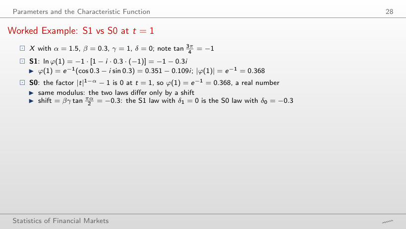
                  Slide 28: Worked Example: S1 vs S0 at t = 1
                  Slide 28

                  The location gap between S0 and S1

                  Worked example: φ(t) in S1 and in S0

                  \[\begin{gathered}\text{S1: } \ln\varphi(t) = -|t|^\alpha\Big[1 - i\beta\,\mathrm{sign}(t)\tan\frac{\pi\alpha}{2}\Big],\\ \text{S0: } \ln\varphi(t) = -|t|^\alpha\Big[1 + i\beta\,\mathrm{sign}(t)\tan\frac{\pi\alpha}{2}\big(|t|^{1-\alpha} - 1\big)\Big],\\ \gamma = 1, \qquad \delta_0 = \delta_1 + \beta\gamma\tan\frac{\pi\alpha}{2}\end{gathered}\]
                      Question for the room On the slide, α = 1.5 and β = 0.3 give δ0 − δ1 = −0.3. The ▶ button raises α from 1.1 to 1.9, with β = 0.3. For which value is the gap between the two locations larger in absolute value: α = 1.1 or α = 1.9?
                      Answer

                      For α = 1.1: β tan(πα/2) = 0.3 × (−6.314) = −1.894, against 0.3 × (−0.158) = −0.048 for α = 1.9. The tangent goes to infinity as α approaches 1, which is why the S1 parameterisation moves the density a lot around α = 1 and S0 does not. The modulus |φ(t)| = e−|t|α is the same in both parameterisations; only the argument differs, by a term linear in t.

                      Tails and Moments

                      Tails on Log-Log Axes
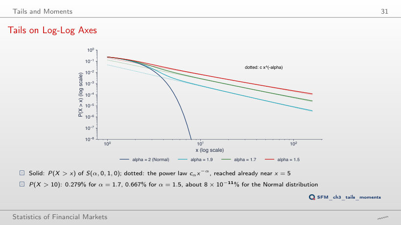
                      Slide 31: Tails on Log-Log Axes
                      Slide 31
                        Question for the room For α = 1.9, P(X > 10) = 0.064%. What is P(X > 20)?
                        Answer

                        0.0165%: doubling the threshold divides the probability by about 21.9 = 3.7 (the exact ratio is 0.256, the power law gives 2−1.9 = 0.268). With α close to 2 the tail is still a power law, far from the Normal distribution, for which P(X > 10) is of the order of 10−12.

                        Instability of the Sample Variance
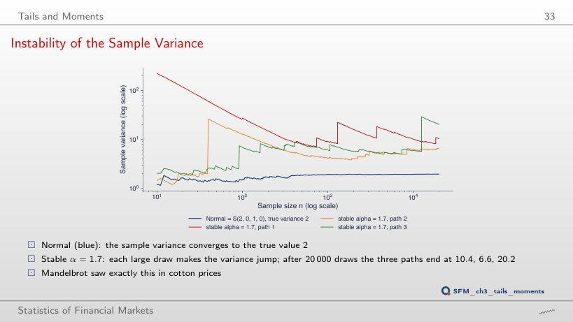
                        Slide 33: Instability of the Sample Variance
                        Slide 33
                          Question for the room The ▶ button takes α from 1.1 to 2. For α = 1.9, do the three sample variances end near 2 after 20,000 draws, as for the Normal distribution?
                          Answer

                          No: 3.16, 2.62 and 4.12, against 1.96 for the Normal distribution. For any α < 2 the variance is infinite and each large draw makes a jump. With α = 1.95 the final values are 2.46, 2.22 and 2.83; only α = 2 gives 2.00, 1.97 and 1.99. With α = 1.7 (the slide): 10.4, 6.6 and 20.2.

                          Tail Probabilities: Stable vs Normal
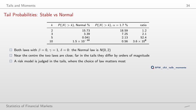
                          Slide 34: Tail Probabilities: Stable vs Normal
                          Slide 34

                          P(|X| > k): the Normal distribution N(0, 2) and the stable law S(α, 0, 1, 0)

                            Question for the room On the slide, for α = 1.7 and k = 10, P(|X| > k) is 0.56%. What does the power law 2cαk−α, with c1.7 = 0.1313, give?
                            Answer

                            0.52%, that is 94% of the exact value. At k = 20 the approximation gives 0.161% against 0.166% exact (97%), and at k = 2 only 8.1% against 18.6%: the tail formula is asymptotic and becomes accurate far in the tail. The ratio to the Normal distribution N(0, 2) is 1.2 at k = 2 and 3.6 × 10⁹ at k = 10.

                            Simulation

                            Worked Example: One Draw Step by Step
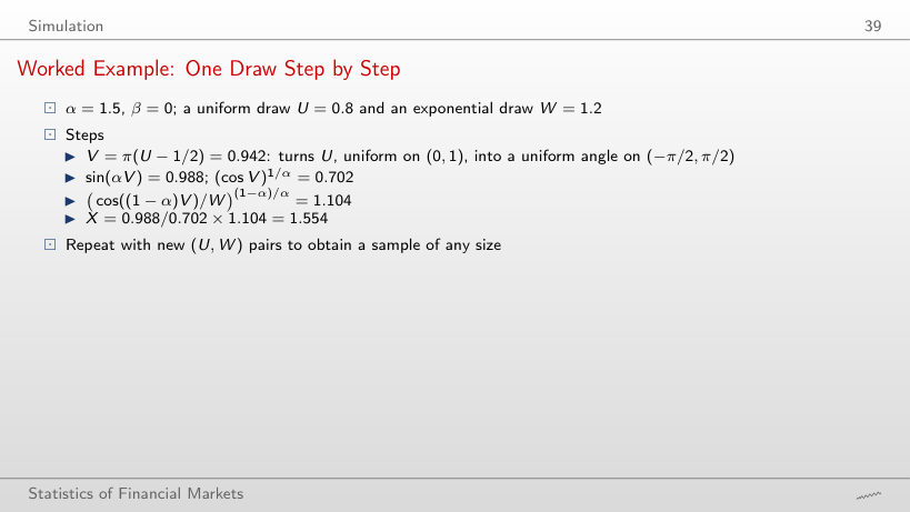
                            Slide 39: Worked Example: One Draw Step by Step
                            Slide 39

                            Worked example: one CMS draw from (U, W)

                            \[\begin{gathered}V = \pi\big(U - \tfrac12\big), \qquad B = \frac{\arctan(\beta\tan\frac{\pi\alpha}{2})}{\alpha}, \qquad S = \Big(1 + \beta^2\tan^2\frac{\pi\alpha}{2}\Big)^{1/(2\alpha)},\\ X = S\,\frac{\sin(\alpha(V + B))}{(\cos V)^{1/\alpha}}\left(\frac{\cos(V - \alpha(V + B))}{W}\right)^{(1-\alpha)/\alpha} \sim S(\alpha, \beta, 1, 0; 1)\end{gathered}\]
                                Question for the room On the slide, U = 0.8 and W = 1.2 give X = 1.554 for α = 1.5 and β = 0. What does X become if W rises to 2, with the same U?
                                Answer

                                1.843. For β = 0, W enters only through the factor (cos((1 − α)V)/W)(1 − α)/α; the exponent (1 − α)/α = −1/3 is negative, so X grows in proportion to W1/3: 1.554 × (2/1.2)1/3 = 1.843. A smaller W shrinks the draw: W = 0.5 gives 1.161. For α = 2 the formula becomes 2 sin V √W, a draw from N(0, 2): 1.772 for U = 0.8 and W = 1.2.

                                CMS Draws against the Exact Density
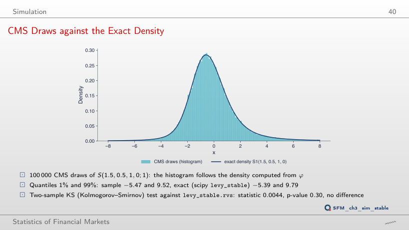
                                Slide 40: CMS Draws against the Exact Density
                                Slide 40
                                  Question for the room For α = 1.5 and β = 0.5, the exact 1% and 99% quantiles are −5.39 and 9.79 (the FFT grid of the chart gives −5.40 and 9.76). What do they become for β = −0.5?
                                  Answer

                                  Mirrored: −9.79 and 5.39 exactly, −9.81 and 5.38 on the FFT grid of the chart (in the simulated sample −9.99 and 5.21). In S1 with δ = 0, the law with −β is the law with β reflected about 0, so β changes which tail is longer, not only the location. The histogram follows the exact density for every combination of α and β.

                                  Estimation

                                  McCulloch's Map from ν_α to α
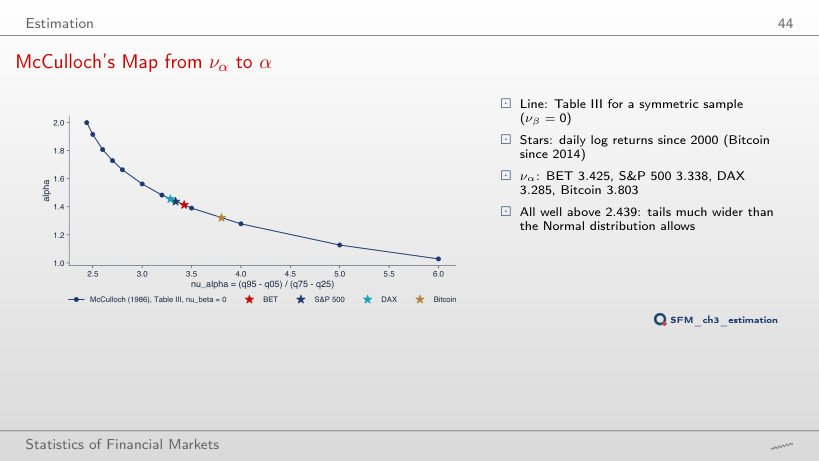
                                  Slide 44: McCulloch's Map from ν_α to α
                                  Slide 44
                                    Question for the room The ▶ button moves the start of the sample from 2000 to 2020. The S&P 500 sample from 2020 has 1,687 days, and the crisis of March 2020 weighs more in it. Does the McCulloch α̂ fall below 1.438?
                                    Answer

                                    No, it rises to 1.543: να falls from 3.338 to 3.044. The McCulloch estimator uses only the 5%, 25%, 50%, 75% and 95% quantiles, so the extreme days do not enter the calculation directly; what matters is how wide the 5–95% band is relative to the interquartile range. The DAX goes from 1.455 to 1.590, BET from 1.414 to 1.480, Bitcoin from 1.322 to 1.400.

                                    Worked Example: McCulloch on the BET
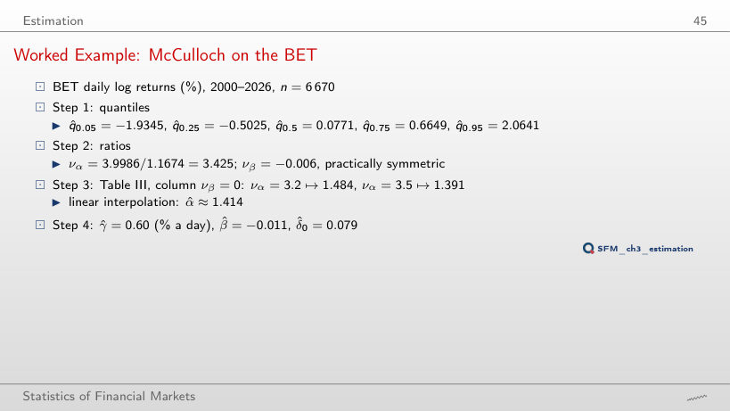
                                    Slide 45: Worked Example: McCulloch on the BET
                                    Slide 45

                                    The McCulloch estimator on daily log returns (%)

                                    Worked example: from the quantiles to α̂, β̂, γ̂ and δ̂0

                                    \[\begin{gathered}\nu_\alpha = \frac{\hat q_{0.95} - \hat q_{0.05}}{\hat q_{0.75} - \hat q_{0.25}}, \qquad \nu_\beta = \frac{\hat q_{0.95} + \hat q_{0.05} - 2\hat q_{0.5}}{\hat q_{0.95} - \hat q_{0.05}},\\ \hat\alpha \approx \alpha_j + \frac{\nu_\alpha - \nu_j}{\nu_{j+1} - \nu_j}\,(\alpha_{j+1} - \alpha_j), \qquad \hat\gamma = \frac{\hat q_{0.75} - \hat q_{0.25}}{\phi_3(\hat\alpha, \hat\beta)}\end{gathered}\]
                                        Question for the room On the slide, να = 3.425 of the BET gives α̂ = 1.414. The ▶ button moves the start of the sample; from 2010, να of the BET falls to 3.082. What α̂ does Table III give?
                                        Answer

                                        About 1.53: between να = 3.0 ↦ 1.563 and να = 3.2 ↦ 1.484, linear interpolation gives 1.531, and with |νβ| = 0.036 the result is α̂ = 1.529. A smaller να means a narrower 5–95% band relative to the interquartile range, hence thinner tails and a larger α̂. The Normal distribution has να = 2.439 and α = 2.

                                        McCulloch vs ML in a Monte Carlo Study
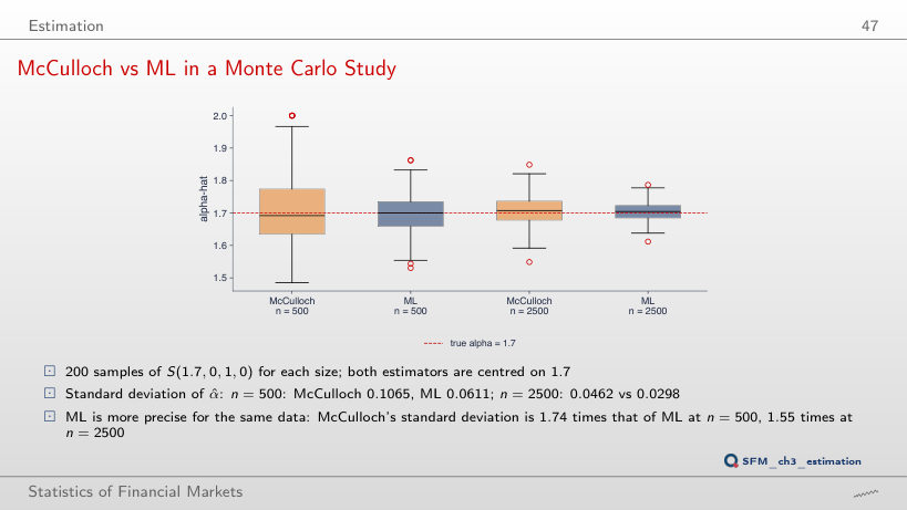
                                        Slide 47: McCulloch vs ML in a Monte Carlo Study
                                        Slide 47

                                        Mean and standard deviation of α̂, α = 1.7

                                          Question for the room The ▶ button raises the number of Monte Carlo samples from 10 to 200. Does the standard deviation of the ML α̂ for n = 500 change between 100 and 200 samples?
                                          Answer

                                          Yes: from 0.050 to 0.061. The precision of α̂ depends on the sample size n; the number of Monte Carlo samples only determines how well this precision is measured. With 100 samples, the estimated standard deviation still has a relative error of at least 1/√(2 × 100) = 7%. For McCulloch, 0.110 at 100 and 0.107 at 200.

                                          Fitting Real Returns

                                          Stable Fits of Daily Log Returns
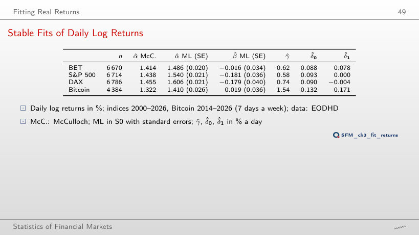
                                          Slide 49: Stable Fits of Daily Log Returns
                                          Slide 49

                                          Stable laws (S0) fitted to daily log returns

                                          Worked example: the location from S0 to S1

                                          \[\delta_1 = \delta_0 - \beta\gamma\tan\frac{\pi\alpha}{2} \qquad (\alpha \ne 1)\]
                                              Question for the room At 95%, the ML interval for α of the S&P 500 is [1.499, 1.581], and the McCulloch α̂ is 1.438, below the interval. For how many of the four series is the McCulloch α̂ below the 99% ML interval?
                                              Answer

                                              For all four. At 99% (±2.576 standard errors) the intervals are BET [1.435, 1.537], S&P 500 [1.486, 1.594], DAX [1.551, 1.661] and Bitcoin [1.343, 1.476], and the McCulloch α̂ is 1.414, 1.438, 1.455 and 1.322. Not even at 99.9% does the conclusion change (Bitcoin: lower bound 1.324). The two methods weigh the tails differently. The intervals are asymptotic and do not include the uncertainty of the McCulloch estimate.

                                              Fitted Densities on a Log Scale
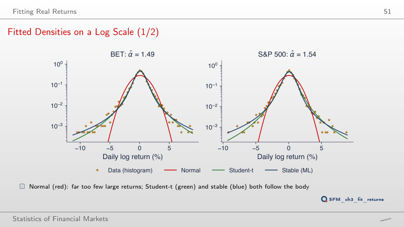
                                              Slide 51: Fitted Densities on a Log Scale
                                              Slide 51
                                                Question for the room At x = −6 standard deviations (−7.28% per day for the S&P 500), how many times smaller is the density of the fitted Normal distribution than the Student-t density?
                                                Answer

                                                About 120,000 times: 4.4 × 10⁻⁹ against 5.5 × 10⁻⁴. The stable density is 1.0 × 10⁻³, almost twice the Student-t density. The Normal tail falls as e−x²/2, the other two as a power of x, so the ratio grows very fast with |x|.

                                                Fitted Densities on a Log Scale
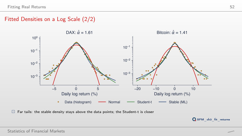
                                                Slide 52: Fitted Densities on a Log Scale
                                                Slide 52
                                                  Question for the room At x = −8 standard deviations for the DAX (−11.26% per day), how many times larger is the stable density than the Student-t density?
                                                  Answer

                                                  About 2.9 times: 3.7 × 10⁻⁴ against 1.3 × 10⁻⁴. The stable tail falls as |x|−α̂−1 with α̂ = 1.61, the Student-t tail as |x|−ν̂−1 with ν̂ = 3.09; a smaller exponent means a heavier tail. The ratio is 1.6 at −5 standard deviations and 3.9 at −10.

                                                  QQ Plots against the Three Models
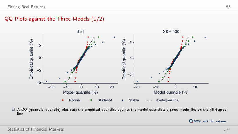
                                                  Slide 53: QQ Plots against the Three Models
                                                  Slide 53
                                                    Question for the room The ▶ button lowers the level p from 5% to 0.1%. At p = 0.1%, what VaR does the fitted stable law give for the S&P 500, against 7.22% in the data?
                                                    Answer

                                                    19.70%, 2.7 times the empirical quantile. The Student-t gives 8.58%, the Normal distribution 3.72%. At p = 1%, the values are 3.45% (data), 4.54% (stable), 3.46% (Student-t) and 2.80% (Normal): the stable law already overstates, but the gap grows as p gets smaller.

                                                    QQ Plots against the Three Models
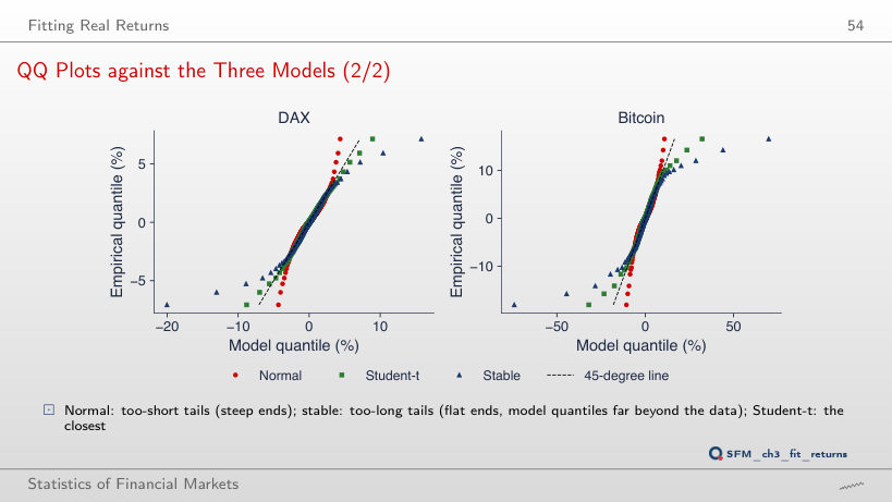
                                                    Slide 54: QQ Plots against the Three Models
                                                    Slide 54
                                                      Question for the room At p = 1%, the VaR of Bitcoin in the data is 10.51%. Which fitted model gives the closest value?
                                                      Answer

                                                      The Student-t: 11.06%. The stable law gives 14.26%, the Normal distribution 7.99%. At p = 0.1%, the data give 18.05%, the Student-t 31.95% and the stable law 74.16%: the Student-t also overstates the far tail of Bitcoin, but much less than the stable law.

                                                      The Left Tail on Log-Log Axes
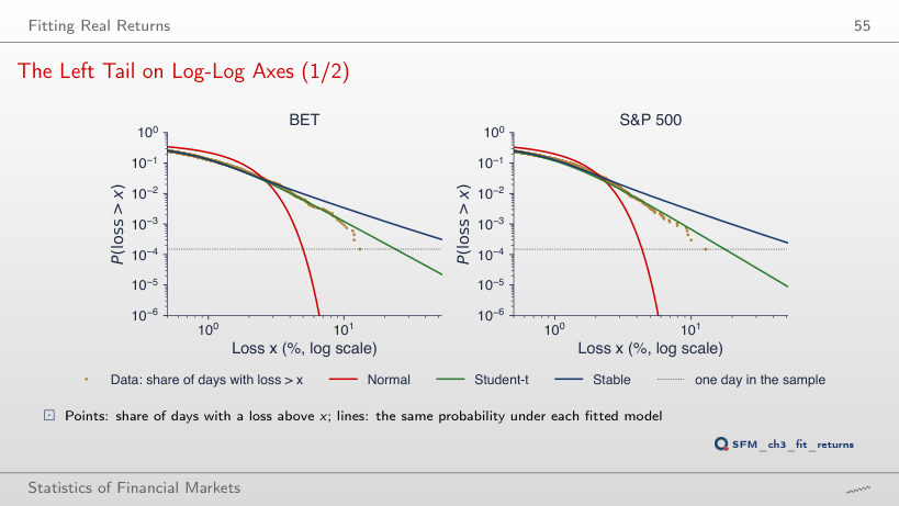
                                                      Slide 55: The Left Tail on Log-Log Axes
                                                      Slide 55
                                                        Question for the room The S&P 500 has 23 days with losses above 5% in 6,714 days. How many such days does the fitted stable law expect?
                                                        Answer

                                                        57.3, 2.5 times as many. The Student-t expects 27.0, the Normal distribution 0.1. For losses above 10%: one day observed, 4.5 under the Student-t and 19.1 under the stable law. The ratio between the days expected by the stable law and those observed grows with the threshold.

                                                        The Left Tail on Log-Log Axes
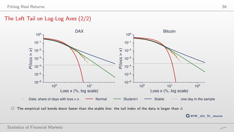
                                                        Slide 56: The Left Tail on Log-Log Axes
                                                        Slide 56
                                                          Question for the room Bitcoin has 4 days with losses above 20% in 4,384 days. How many days do the Student-t and the stable law expect?
                                                          Answer

                                                          12.3 under the Student-t and 26.9 under the stable law; the Normal distribution gives practically zero. Both heavy-tailed models overstate the far tail of Bitcoin, the stable law more than 6 times. For losses above 10%: 56 observed, 54.2 (Student-t), 73.9 (stable).

                                                          Counting Large Losses
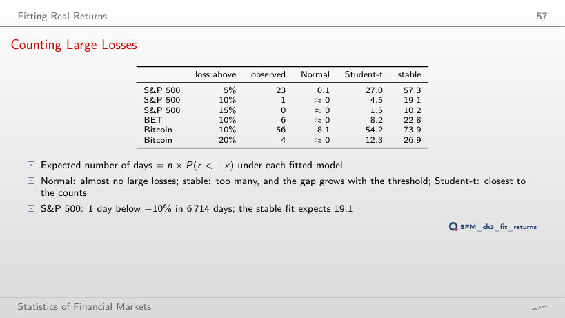
                                                          Slide 57: Counting Large Losses
                                                          Slide 57

                                                          Days with losses above x%: observed and expected (n × P(r < −x)) under each fitted model

                                                          Worked example: the power-law tail of the fitted stable law

                                                          \[\begin{gathered}P(r_t < -x) = P\Big(Z < -\frac{x + \hat\delta_0}{\hat\gamma}\Big) \approx c_\alpha (1 - \hat\beta)\Big(\frac{x + \hat\delta_0}{\hat\gamma}\Big)^{-\hat\alpha}, \qquad c_\alpha = \frac{\Gamma(\alpha)\sin(\pi\alpha/2)}{\pi},\\ Z \sim S(\hat\alpha, \hat\beta, 1, 0; 0), \qquad E = n\,P(r_t < -x)\end{gathered}\]
                                                              Question for the room The stable law fitted to the S&P 500 expects 19.1 days with losses above 10% in 6,714 days. How many days does the power-law tail approximation cα(1 − β̂)z−α̂ give, with z = (10 + δ̂0)/γ̂ = 17.33?
                                                              Answer

                                                              18.3 days, 96% of the exact value: c1.540 = 0.1868, P ≈ 0.1868 × 1.181 × 17.33−1.540 = 0.00273. The factor 1 − β̂ = 1.181 comes from β̂ = −0.181: the left tail of the fitted law is heavier than the right one. Observed: a single day. For Bitcoin at 10%, the approximation gives 68.2 days, against 73.9 exact and 56 observed.

                                                              VaR 1% and VaR 0.1% under the Three Models
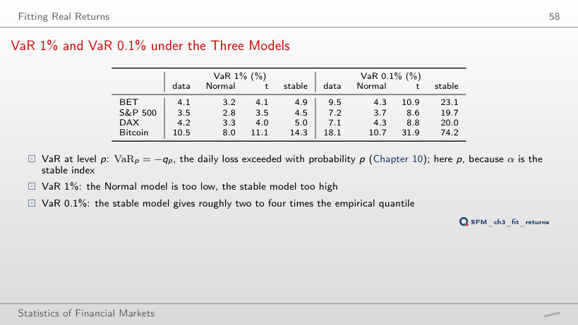
                                                              Slide 58: VaR 1% and VaR 0.1% under the Three Models
                                                              Slide 58

                                                              VaRp = −qp from the data and from the three fitted models (% a day)

                                                              Worked example: VaR from the fitted stable law and from the Normal distribution

                                                              \[\begin{gathered}\mathrm{VaR}_p = -q_p: \qquad \text{Normal: } -(\hat\mu + \hat\sigma z_p), \quad z_p = \Phi^{-1}(p);\\ \text{stable: } -(\hat\delta_0 + \hat\gamma\, z^{S}_p), \quad z^{S}_p = F^{-1}_{S(\hat\alpha, \hat\beta, 1, 0; 0)}(p)\end{gathered}\]
                                                                  Question for the room At VaR 1% for the S&P 500, the stable law gives 4.54%, 1.62 times the VaR of the Normal distribution (2.80%). The ▶ button lowers the level of the second group of columns. What does the stable/Normal ratio become at VaR 0.05%?
                                                                  Answer

                                                                  About 7.9: 31.21% against 3.97%. The ratio grows as p falls, because the quantile of the stable law grows like p−1/α and the Normal one only like √(2 ln(1/p)). The empirical quantile at 0.05% is 9.31%, so the stable law exceeds the data 3.4 times. At 5% the stable/Normal ratio is 0.91: in the body of the distribution, the stable law gives a smaller VaR.

                                                                  Comparison of the Three Models
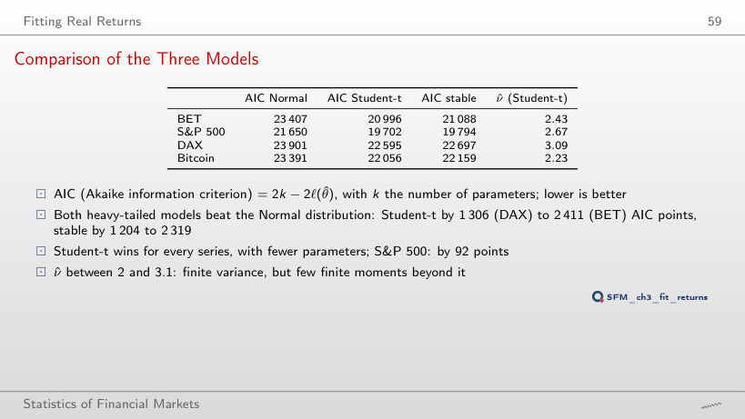
                                                                  Slide 59: Comparison of the Three Models
                                                                  Slide 59

                                                                  Information criteria of the three fitted models

                                                                    Question for the room On the slide, AIC prefers the Student-t to the stable law by 92 points for the S&P 500. What does the gap become with BIC = k ln n − 2ℓ?
                                                                    Answer

                                                                    98.4 points. The stable law has one more parameter (4 against 3), and BIC penalises it by ln 6,714 = 8.81 instead of 2: 91.6 + 6.8 = 98.4. The conclusion does not change. Against the Normal distribution, the AIC gains of the Student-t lie between 1,306 (DAX) and 2,411 (BET) points, those of the stable law between 1,204 and 2,319, as on the slide.

                                                                    Critique of the Stable Model: Finite or Infinite Variance

                                                                    Test 1: Stability of α under Aggregation
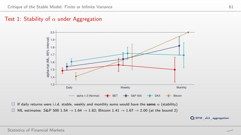
                                                                    Slide 61: Test 1: Stability of α under Aggregation
                                                                    Slide 61
                                                                      Question for the room On the slide, the 95% intervals of the ML α̂ for the S&P 500 at the daily (1.54) and monthly (1.82) horizon do not overlap. Do they overlap at the 99% confidence level?
                                                                      Answer

                                                                      No. At 99% (±2.576 standard errors), the daily interval is [1.486, 1.594] and the monthly one [1.655, 1.984]. Not even at 99.9% (±3.29 standard errors) do they overlap, although the gap between them almost vanishes. For the DAX and BET the intervals already overlap at 95%. The intervals are asymptotic, and the monthly one rests on 321 months.

                                                                      Test 2: Convergence of the Sample Variance
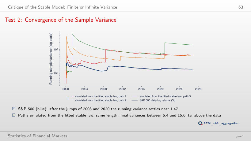
                                                                      Slide 63: Test 2: Convergence of the Sample Variance
                                                                      Slide 63
                                                                        Question for the room For Bitcoin (α̂ = 1.410), the running variance of the data at the end of the sample is 12.14. Where do the final variances of the three paths simulated from the fitted stable law end?
                                                                        Answer

                                                                        Much higher: 252.1, 111.4 and 52.6, 4 to 21 times the variance of the data. The same holds for the S&P 500 (the slide): data 1.47, paths 5.9, 5.4 and 15.6. A stable law with α̂ < 2 produces extremes that the real series do not have, and their sample variance does not settle.

                                                                        Daily log returns, in %: BET, S&P 500 and DAX from January 2000, Bitcoin from September 2014 (7 days a week), to 18 September 2026. EODHD closing prices. The fitted laws are those of the lecture: the Normal distribution, the Student-t and the stable law fitted by maximum likelihood in the S0 parameterisation.