

Statistics of Financial Markets

Chapter 5 · Heavy Tails and Extreme Value Theory

The slide of the lecture is on the left, the same figure on the right, computed in the browser from the same data. The ▶ button moves the parameter step by step.

The Importance of Tails · Heavy Tails and Regular Variation · The Hill Estimator · The Mean Excess Function · Block Maxima and the GEV Distribution · Peaks over Threshold and the GPD · VaR and ES by Extreme Value Theory

The Importance of Tails

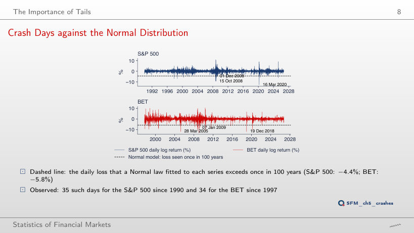
Crash Days against the Normal Distribution
Slide 8: Crash Days against the Normal Distribution
Slide 8
    Question for the room Below the level of the loss exceeded once in 100 years under the Normal distribution, the S&P 500 has 35 days since 1990. The ▶ button moves the period T from 1 year to 10,000 years. How many S&P 500 days are below the level of a "once in 10,000 years" loss?
    Answer

    17 days, below −5.56%. The Normal distribution expects 0.0037 such days in 9,240 (probability 1/(10,000 × 252) per day). The level only moves from −4.44% to −5.56%: the tail of the Normal distribution falls so fast that a period 100 times longer moves the threshold by little more than one percentage point. BET has 22 days below its 10,000-year level (−7.25%). At T = 1 year, the S&P 500 has 120 days below −2.98%, against 36.7 expected.

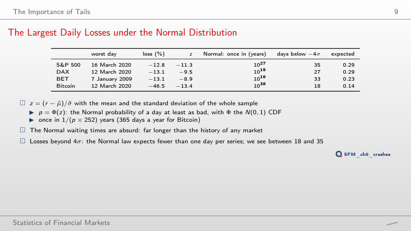
    The Largest Daily Losses under the Normal Distribution
    Slide 9: The Largest Daily Losses under the Normal Distribution
    Slide 9

    Worked example: the Normal return period

    \[z = \frac{r - \hat\mu}{\hat\sigma}, \qquad p = \Phi(z), \qquad \text{once in} \;\; \frac{1}{p \times d} \;\; \text{years} \quad (d = 252;\; 365 \text{ for Bitcoin})\]
        Question for the room At the 4σ threshold, the S&P 500 has 35 days below −4σ, against 0.29 expected under the Normal distribution. The ▶ button raises the threshold up to 6σ. How many S&P 500 days are below −6σ?
        Answer

        11 days. The Normal distribution expects 9,240 × Φ(−6) = 9.1 × 10⁻⁶ days, i.e. one such day in 4 million years. The 35 days below −4σ do not thin out as the Normal shape would have them (35 × Φ(−6)/Φ(−4) = 0.001): a third of them lie beyond 6σ. DAX has 5 days below −6σ, BET 13, Bitcoin 2.

        Heavy Tails and Regular Variation

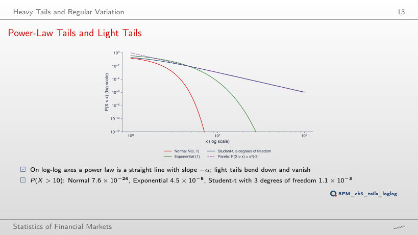
        Power-Law Tails and Light Tails
        Slide 13: Power-Law Tails and Light Tails
        Slide 13
          Question for the room At x = 10, P(X > 20)/P(X > 10) = 0.128 for the Student-t distribution with 3 degrees of freedom. What does the ratio P(X > 2x)/P(X > x) of the Student-t become at x = 50?
          Answer

          0.125 = 2−3: for a regularly varying tail, P(X > tx)/P(X > x) → t−α, with α = 3 for the Student-t with 3 degrees of freedom. At x = 2 the ratio is still 0.201, at x = 20 it is 0.126. For the exponential distribution the ratio is e−x, 1.9 × 10⁻²² at x = 50, and for the Normal distribution about 10−1629: light tails vanish at every doubling of the threshold, the power-law tail always loses the same factor 8.

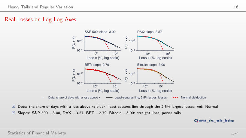
          Real Losses on Log-Log Axes
          Slide 16: Real Losses on Log-Log Axes
          Slide 16
            Question for the room Through the largest 2.5% of the losses, the slope of the S&P 500 is −3.00. The ▶ button raises the share to 10%. What slope does the line through the largest 10% of the losses give?
            Answer

            −2.50: the line reaches into the body of the distribution, where the points bend and flatten the line. At 10%, the Hill estimator also falls, to 2.04. DAX: from −3.57 to −2.65; BET: −2.17; Bitcoin: −2.31. At 0.5% (46 losses for the S&P 500), the slope of the DAX is −4.39: few points, high variability. The power law describes only the tail, and the estimate depends on how many losses enter it.

            The Hill Estimator

            Worked Example: Hill on Six Losses
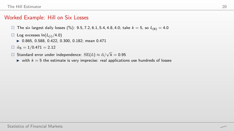
            Slide 20: Worked Example: Hill on Six Losses
            Slide 20

            The largest daily losses and the threshold X(k+1)

            Worked example: the Hill estimator on the real losses

            \[\hat\xi = \frac{1}{k}\sum_{i=1}^{k} \ln\frac{X_{(i)}}{X_{(k+1)}}, \qquad \hat\alpha = \frac{1}{\hat\xi}, \qquad \mathrm{SE}(\hat\alpha) \approx \frac{\hat\alpha}{\sqrt{k}}\]
                Question for the room On the slide, six illustrative losses give α̂ = 2.12. For the six largest real losses of the S&P 500 (k = 5, threshold X(6) = 7.92%), what is α̂?
                Answer

                4.15: the log ratios are 0.477, 0.232, 0.178, 0.166 and 0.152, with sum 1.205, so ξ̂ = 0.241 and α̂ = 1/0.241 = 4.15. Four of the five losses (9.99% … 9.22%) are close to each other, and the largest ratio comes from 16 March 2020 alone. SE = 4.15/√5 = 1.86: the i.i.d. 95% interval, [0.51, 7.78], also contains the estimate at k = 2.5% of n (2.97). With five losses, α̂ is not precise.

                Hill Plots of Daily Losses
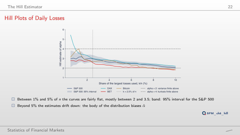
                Slide 22: Hill Plots of Daily Losses
                Slide 22
                  Question for the room At k = 2.5% of n, α̂ of the S&P 500 is 2.97, with the 95% interval [2.59, 3.35]. The ▶ button moves k/n from 0.5% to 10%. What is α̂ of the S&P 500 at k = 10% of n?
                  Answer

                  2.04, with the i.i.d. interval [1.91, 2.18], which no longer contains 2.97. With a large k the body of the distribution enters and biases the estimate downwards; the interval narrows (SE = α̂/√k), so a large k gives a precise estimate of a biased quantity. BET falls to 1.82, below 2, although it is 2.57 in the flat zone. The i.i.d. interval also understates the uncertainty: at k = 2.5%, the i.i.d. SE of the S&P 500 is 0.20 and the moving-block bootstrap SE (blocks of 20 days) 0.30, 1.5 times larger, because large losses come in clusters; for the DAX the two coincide (0.20).

                  Hill Estimates for Four Markets
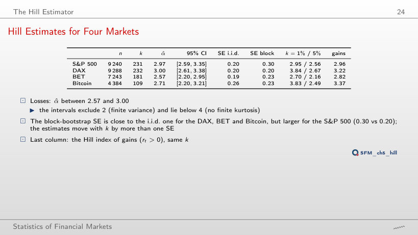
                  Slide 24: Hill Estimates for Four Markets
                  Slide 24
                    Question for the room The last column is the Hill index of the gains, with the same k. For the S&P 500, the losses have α̂ = 2.97 at k = 2.5% of n. What is α̂ of the gains?
                    Answer

                    2.96: for the S&P 500 the gains have a tail as heavy as the losses. The largest gains are the rebounds of the same crises: 10.96% (13 October 2008), 10.25% (28 October 2008), 9.09% (9 April 2025), 8.97% (24 March 2020). DAX (3.22), BET (2.82) and Bitcoin (3.37) have gains with lighter tails than their losses. Also at k = 2.5% of n, the block SE of the S&P 500 is 0.30, 1.5 times the i.i.d. SE (0.20), because large losses come in clusters; for the DAX the two coincide (0.20).

                    Four Stocks of the Bucharest Stock Exchange
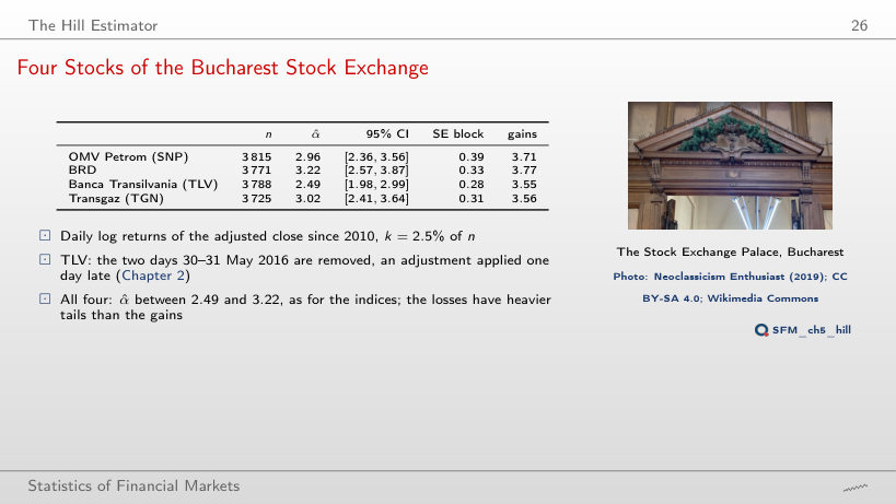
                    Slide 26: Four Stocks of the Bucharest Stock Exchange
                    Slide 26
                      Question for the room At k = 2.5% of n, none of the four BVB stocks has α̂ below 2.4 (the smallest is TLV, 2.49). The ▶ button moves k/n from 1% to 10%. How many of them have α̂ below 2.4 at k = 10% of n?
                      Answer

                      All four: SNP 2.27, BRD 2.35, TLV 2.08, TGN 1.87. With 10% of n the body of the distribution enters the estimate and biases it downwards, as for the indices (S&P 500 2.04). The intervals narrow (i.i.d. SE between 0.10 and 0.12), but they are intervals around a biased quantity. At 1% of n, BRD has 3.86, with the interval [2.62, 5.11]: few losses, high variability.

                      Hill Plots of the BVB Stocks
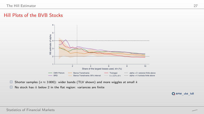
                      Slide 27: Hill Plots of the BVB Stocks
                      Slide 27
                        Question for the room At k = 2.5% of n, TLV has α̂ = 2.49 and the 95% interval [1.98, 2.99], 1.01 wide. With n = 3,788, k = 1% of n means 37 losses. How wide is the TLV interval at k = 1% of n?
                        Answer

                        1.96, from 2.07 to 4.03, almost twice as wide. The width of the interval is 2 × 1.96 α̂/√k: k falls from 94 to 37 (√(94/37) = 1.59), and α̂ rises from 2.49 to 3.05. The BVB samples are 2.5 times shorter than those of the indices, so the same k/n gives fewer losses and wider bands; the S&P 500 has the interval [2.35, 3.56] at k = 1%. In the flat zone (1%–5%), none of the four stocks has α̂ below 2.

                        The Mean Excess Function

                        Empirical Mean Excess of Daily Losses
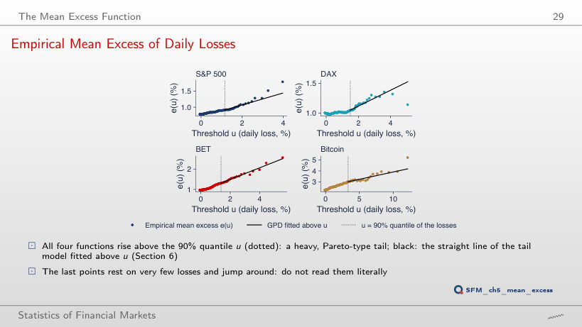
                        Slide 29: Empirical Mean Excess of Daily Losses
                        Slide 29
                          Question for the room At the threshold u = 90% quantile (1.16%), the mean excess of the S&P 500 losses is 0.92%. The ▶ button raises the threshold from the 80% to the 98% quantile. What is e(u) at the 98% quantile (u = 2.52%)?
                          Answer

                          1.22%: the mean excess grows with the threshold, as a heavy tail requires. For a Pareto tail, e(u) = u/(α − 1) grows linearly; for the exponential distribution it would be constant, for the Normal distribution it would fall towards 0. BET: from 1.30% to 1.79%. At the 98% quantile, the GPD is fitted to only 185 excesses of the S&P 500 (against 924 at 90%), and ξ̂ rises from 0.158 to 0.255: noisier estimates, as the last points of the chart also show.

                          Reading the Mean Excess Plot
                          Slide 30: Reading the Mean Excess Plot
                          Slide 30
                            Question for the room At the 90% threshold, the mean excess of the S&P 500 is 0.92%, and e(u)/u = 0.79. The ▶ button raises the threshold up to the 98% quantile (u = 2.52%). What does e(u)/u become?
                            Answer

                            0.48: e(u) grows, to 1.22%, but more slowly than the threshold. For a Pareto tail, e(u)/u = 1/(α − 1): the ratio 0.48 corresponds to α = 1 + 1/0.48 = 3.1, close to the Hill estimate (2.97); the ratio 0.79 at 90% would give α = 2.3, because there the losses of the body still matter. BET: from 0.95 to 0.52.

                            Block Maxima and the GEV Distribution

                            The Three Extreme Value Laws
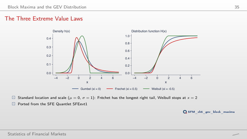
                            Slide 35: The Three Extreme Value Laws
                            Slide 35
                              Question for the room With ξ = −0.5, the Weibull distribution stops at x = 2. Where does it stop for ξ = −0.25?
                              Answer

                              At x = 4: the upper endpoint is μ − σ/ξ = 0 − 1/(−0.25). As |ξ| falls towards 0, the endpoint moves away and the Weibull distribution approaches the Gumbel; the Fréchet distribution with ξ = 0.25 has tail index 1/ξ = 4, and P(X > 5) falls from 0.078 (ξ = 0.5) to 0.038, against 0.0067 for the Gumbel. The sign of ξ decides the type of tail, its size decides how heavy or how short it is.

                              The Theorem in a Simulation
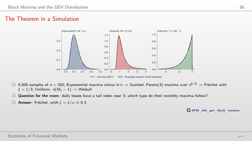
                              Slide 36: The Theorem in a Simulation
                              Slide 36
                                Question for the room With n = 250, the mean of the exponential maxima minus ln n is 0.568, close to the mean of the Gumbel law, 0.577 (the Euler–Mascheroni constant). The ▶ button goes through n = 2, 5, 10, 21, 50, 100, 250. What is the mean for n = 2?
                                Answer

                                0.837 in the simulation; exactly, E[M2] − ln 2 = 1 + 1/2 − 0.693 = 0.807. In general E[Mn] = 1 + 1/2 + … + 1/n, and its difference from ln n tends to 0.577: the convergence to the Gumbel is slow, of order 1/n. For the uniform distribution, the mean of n(M − 1) is exactly −n/(n + 1): −0.667 at n = 2, almost −1 at n = 250. At n = 21 (one trading month) the means are already 0.593, 1.373 and −0.957. The values n ≠ 250 are extra runs of the lecture's code, with the same seed.

                                GEV Fits to Monthly Maxima
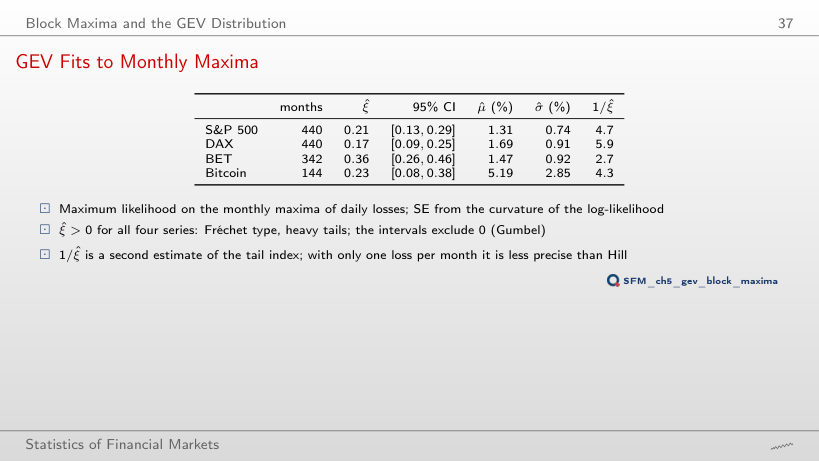
                                Slide 37: GEV Fits to Monthly Maxima
                                Slide 37
                                  Question for the room With monthly maxima, ξ̂ of BET is 0.36. The ▶ button goes through weekly, monthly, quarterly and yearly maxima. What is ξ̂ of BET with weekly maxima?
                                  Answer

                                  0.05, with the interval [0.03, 0.07]. A block of 5 days is far from the limit of the Fisher–Tippett–Gnedenko theorem: 7% of the weekly maxima of BET are gains (no loss day in the week), and the fit follows the body of the distribution. With quarterly blocks, ξ̂ = 0.42; with yearly blocks only 28 maxima remain, and the interval [−0.19, 0.65] also contains 0. The block must be long enough for the theorem and short enough to leave many maxima.

                                  Goodness of Fit of the GEV: PP and QQ Plots
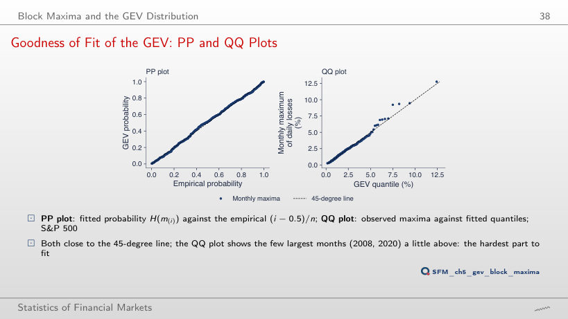
                                  Slide 38: Goodness of Fit of the GEV: PP and QQ Plots
                                  Slide 38
                                    Question for the room In the QQ plot of the GEV, the month with the largest loss of the S&P 500 (March 2020, 12.77%) has the fitted quantile 12.43%. The ▶ button switches to the Gumbel fit (ξ = 0). What fitted quantile does the same month get?
                                    Answer

                                    6.99%: an exponential tail puts the most extreme month at half its observed value, and the top points of the QQ plot rise far above the diagonal. The 10-year level falls from 7.4% (GEV) to 5.3% (Gumbel), a level exceeded in 12 of the 440 months, more than three times as often as once in 10 years. The Gumbel fit is an extra run, for comparison; the 95% interval of ξ̂ in the lecture, [0.13, 0.29], excludes 0. For BET (ξ̂ = 0.36), the GEV puts the largest month at 26.1%, against 13.1% observed: the fitted tail is heavier than the data.

                                    Return Levels
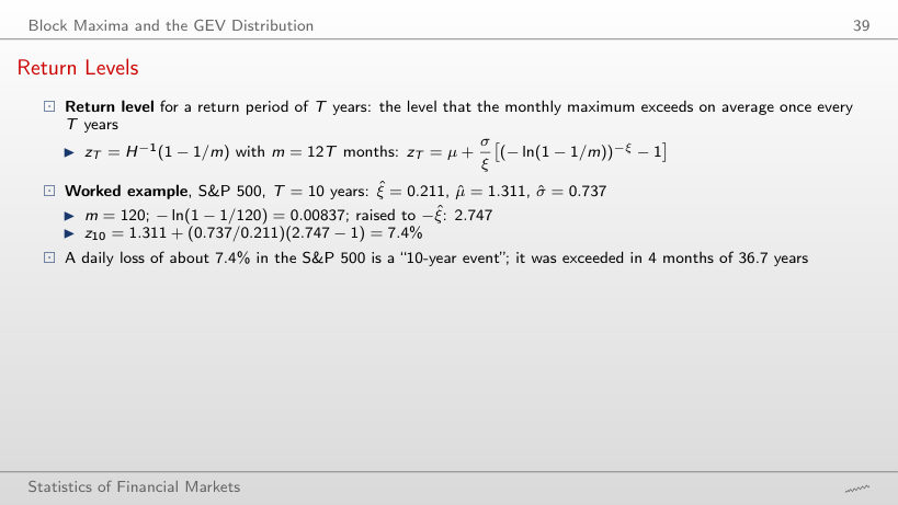
                                    Slide 39: Return Levels
                                    Slide 39

                                    Worked example: a GEV return level

                                    \[z_T = \mu - \frac{\sigma}{\xi}\Big[1 - \big(-\ln(1 - 1/m)\big)^{-\xi}\Big], \qquad m = 12\,T\]
                                        Question for the room For the S&P 500, the 10-year level (7.40%) was exceeded in 4 months of 440, against 440/120 = 3.67 expected. The 1-year level is 3.66%. In how many months was it exceeded?
                                        Answer

                                        In 31 months, against 440/12 = 36.7 expected. "Once a year" means on average one month in 12, i.e. about 37 months in 36.7 years. At T = 1 year: −ln(1 − 1/12) = 0.0870, raised to −0.211 gives 1.675, and z = 1.311 + 3.486 × 0.675 = 3.66%. For the DAX: 36 months above 4.45%, as expected.

                                        Return Level Plot
                                        Slide 40: Return Level Plot
                                        Slide 40
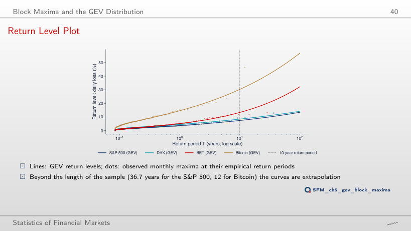
                                          Question for the room The 10-year level of BET is 13.3%, and the largest loss observed in 28.5 years is 13.1%. The ▶ button moves T from 1 to 100 years. What is the 100-year level of BET?
                                          Answer

                                          32.2%, almost 2.5 times the largest observed loss. With ξ̂ = 0.36, the return level grows roughly as Tξ: every multiplication of T by 10 raises the level by a factor of about 2.4. It is an extrapolation to 3.5 times the length of the sample; already at 10 years the bootstrap interval is [10.3%, 17.5%]. S&P 500, with ξ̂ = 0.21: 13.4% at 100 years, close to the largest observed loss (12.8%).

                                          Return Levels of Daily Losses: 1, 10 and 50 Years
                                          Slide 41: Return Levels of Daily Losses: 1, 10 and 50 Years
                                          Slide 41
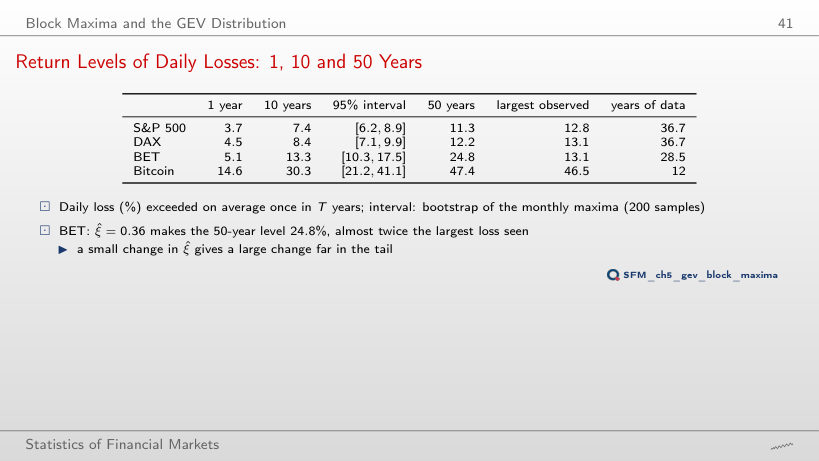
                                            Question for the room At T = 10 years, the bootstrap interval of BET is [10.3%, 17.5%]: the upper bound is 1.70 times the lower one. The ▶ button moves T from 1 to 100 years. What does this ratio become at T = 100 years?
                                            Answer

                                            2.46: the interval is [20.8%, 51.4%], around a level of 32.2%. The larger T, the more the level depends on ξ, and the uncertainty of ξ̂ (interval [0.26, 0.46]) is amplified. For Bitcoin, at 100 years: [31.1%, 94.4%], with 12 years of data. S&P 500 at 100 years: [9.9%, 18.3%].

                                            Peaks over Threshold and the GPD

                                            GPD Densities and Tails
                                            Slide 44: GPD Densities and Tails
                                            Slide 44
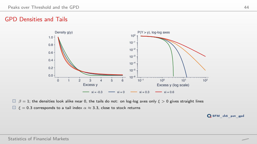
                                              Question for the room With ξ = 0.3, the GPD tail has tail index 1/ξ ≈ 3.3: the mean and the variance of the excess are finite. From which value of ξ does the variance of the excess become infinite?
                                              Answer

                                              From ξ = 1/2: the variance exists only for α = 1/ξ > 2. The mean excess, β/(1 − ξ), exists up to ξ = 1. For ξ = 0.5, P(Y > 10) = 0.028 (β = 1), against 0.0098 for ξ = 0.3 and 4.5 × 10⁻⁵ for ξ = 0. The GPD fits of the lecture have ξ̂ between 0.12 and 0.22 for the four series: heavy tails with finite variance.

                                              Parameter Stability
                                              Slide 46: Parameter Stability
                                              Slide 46
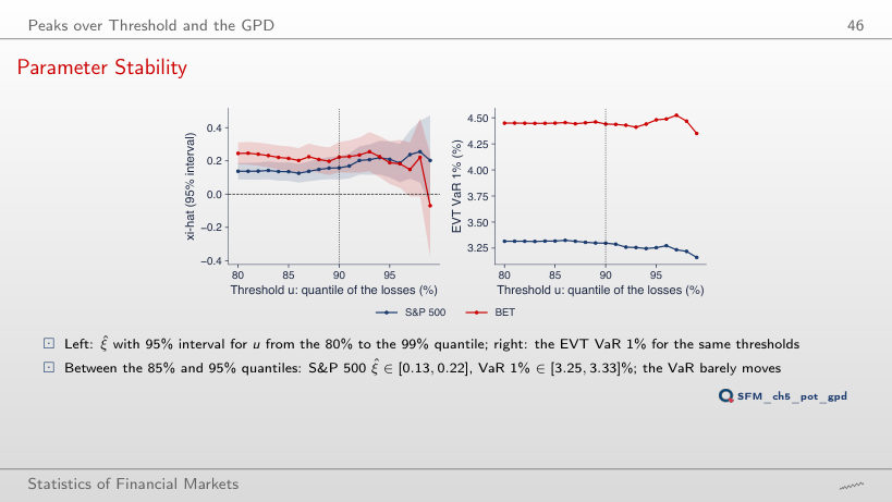
                                                Question for the room At the 90% threshold, ξ̂ of the S&P 500 is 0.158 and the EVT VaR 1% 3.30%. The ▶ button raises the threshold from the 80% to the 99% quantile. What do ξ̂ and VaR 1% become at the 99% threshold (93 excesses)?
                                                Answer

                                                ξ̂ = 0.203, with a 95% interval from −0.07 to 0.47 (SE 0.138, four times larger than at 90%), but VaR 1% stays at 3.16%. VaR 1% lies inside the data (92 days beyond it in the sample), so it depends little on the shape of the tail; ξ̂ depends strongly on the threshold. Between the 85% and 95% quantiles: ξ̂ between 0.13 and 0.22, VaR 1% between 3.25% and 3.33%. BET at 99%: ξ̂ = −0.07, VaR 1% 4.35%.

                                                GPD Fits above the 90% Quantile
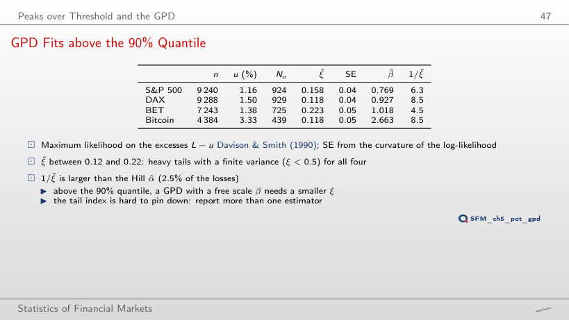
                                                Slide 47: GPD Fits above the 90% Quantile
                                                Slide 47

                                                Worked example: the tail index α = 1/ξ

                                                \[P(L > x) \approx c\,x^{-1/\xi} \;\Rightarrow\; \alpha = \frac{1}{\xi}, \qquad \hat\xi \pm 1.96\,\mathrm{SE} \;\Rightarrow\; \alpha \in \Big[\frac{1}{\hat\xi + 1.96\,\mathrm{SE}},\; \frac{1}{\hat\xi - 1.96\,\mathrm{SE}}\Big]\]
                                                    Question for the room At the 90% threshold, 1/ξ̂ of the DAX is 8.5. The ▶ button raises the threshold from the 80% to the 98% quantile. What does 1/ξ̂ of the DAX become at the 98% threshold (186 excesses)?
                                                    Answer

                                                    About 19: ξ̂ falls to 0.053, with SE 0.075, and the 95% interval [−0.09, 0.20] contains 0. The inverse of an estimate close to 0 is unstable: from the same interval, α can be anywhere above 5.0. At the 80% threshold, DAX has 1/ξ̂ = 15.6; the S&P 500 falls from 6.3 (90%) to 3.9 (98%). The Hill estimate of the DAX (k = 2.5% of n) is 3.00.

                                                    Goodness of Fit of the GPD: PP and QQ Plots
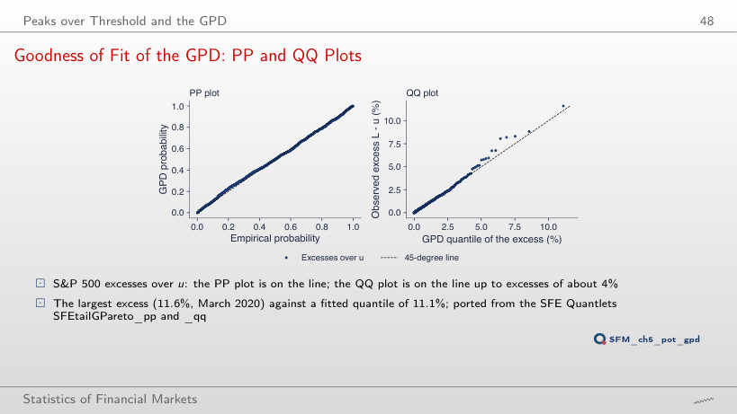
                                                    Slide 48: Goodness of Fit of the GPD: PP and QQ Plots
                                                    Slide 48
                                                      Question for the room At the 90% threshold, the largest excess of the S&P 500 (11.60%, March 2020) is above the fitted GPD quantile (11.11%). The ▶ button raises the threshold from the 80% to the 98% quantile. What happens to this point of the QQ plot at the 98% threshold?
                                                      Answer

                                                      It falls below the diagonal: the excess is 10.24% (the threshold rose to 2.52%), and the fitted quantile 12.65%, because ξ̂ rises to 0.255 on only 185 excesses. The last point of the QQ plot depends strongly on ξ̂, hence on the threshold. For BET, the GPD above the 90% quantile puts the largest excess at 18.56%, against 11.74% observed: the fitted tail is heavier than the largest losses of the sample.

                                                      The Fitted Tails
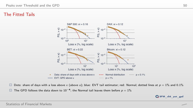
                                                      Slide 50: The Fitted Tails
                                                      Slide 50
                                                        Question for the room The ▶ button lowers the level p from 2.5% to 0.01%. With p = 0.01% (one day in 10,000), what is the VaR of the S&P 500 by EVT and by the Normal distribution?
                                                        Answer

                                                        EVT 10.79%, Normal 4.18%, 2.6 times less. At p = 1%, the ratio is 1.27 (3.30% against 2.60%). The sample of 9,240 days holds on average 0.9 days beyond VaR 0.01%, so the historical quantile (10.21%) is only an interpolation between the two largest losses. The Hill quantile gives 15.02%: far in the tail, the estimators differ a lot. BET: EVT 18.10%, Hill 26.16%, historical 12.24%.

                                                        Waiting Times of the Worst Days: Normal Law and EVT
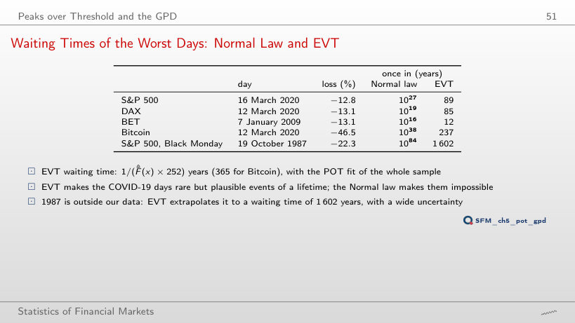
                                                        Slide 51: Waiting Times of the Worst Days: Normal Law and EVT
                                                        Slide 51
                                                          Question for the room With the GPD above the 90% quantile, EVT gives 19 October 1987 a waiting time of 1,602 years. The ▶ button moves the threshold from the 80% to the 98% quantile. What does the waiting time become with the 98% threshold?
                                                          Answer

                                                          About 306 years: ξ̂ of the S&P 500 rises from 0.158 to 0.255, and a heavier tail makes the 22% event much less rare. At the 80% threshold the waiting time is 2,770 years. The farther the loss lies from the data, the more its waiting time depends on the threshold. The DAX moves the other way: 85 years at 90%, 187 at 98%, because its ξ̂ falls to 0.053. The Normal distribution stays at 1084 years for any threshold.

                                                          VaR and ES by Extreme Value Theory

                                                          Worked Example: S&P 500, Step by Step
                                                          Slide 54: Worked Example: S&P 500, Step by Step
                                                          Slide 54

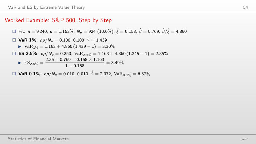
                                                          Worked example: VaR and ES from the GPD

                                                          \[\mathrm{VaR}_p = u + \frac{\beta}{\xi}\Big[\Big(\frac{n}{N_u}\,p\Big)^{-\xi} - 1\Big], \qquad \mathrm{ES}_p = \frac{\mathrm{VaR}_p + \beta - \xi u}{1 - \xi}\]
                                                              Question for the room For the S&P 500, ES 2.5% / VaR 2.5% = 3.49/2.35 = 1.48. The ▶ button lowers the ES level from 5% to 0.01%. What does the ratio ES/VaR become at 0.01%?
                                                              Answer

                                                              1.25: ES 0.01% = 13.52%, VaR 0.01% = 10.79%. Far in the tail, ES/VaR tends to 1/(1 − ξ̂) = 1/(1 − 0.158) = 1.19: the excess over VaR is again GPD with the same ξ, and its mean grows in proportion to VaR. At 2.5% the ratio is larger because the term (β̂ − ξ̂u)/(1 − ξ̂) = 0.695 weighs a lot against a small VaR.

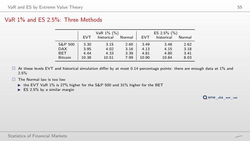
                                                              VaR 1% and ES 2.5%: Three Methods
                                                              Slide 55: VaR 1% and ES 2.5%: Three Methods
                                                              Slide 55
                                                                Question for the room At VaR 1%, EVT gives 3.30% for the S&P 500 and the Normal distribution 2.60%. The ▶ button moves the VaR level through 5%, 2.5%, 1%, 0.5%, 0.1%, 0.05% and 0.01%. At VaR 5%, which method gives the largest VaR for the S&P 500?
                                                                Answer

                                                                The Normal distribution: 1.83%, against 1.73% EVT and 1.72% historical; the same holds for DAX, BET and Bitcoin. Heavy-tailed losses are also more concentrated around 0, so near the body of the distribution the empirical quantile lies below the Normal one with the same standard deviation. From 2.5% on (2.35% EVT, 2.19% Normal) the order reverses, and the gap widens towards the tail.

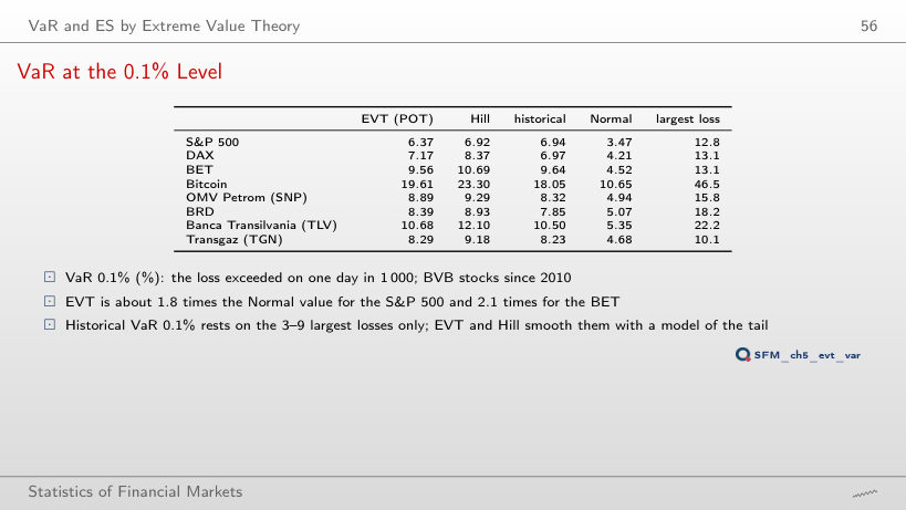
                                                                VaR at the 0.1% Level
                                                                Slide 56: VaR at the 0.1% Level
                                                                Slide 56
                                                                  Question for the room At VaR 0.1%, EVT gives 9.56% for BET, 2.1 times the Normal VaR (4.52%). The ▶ button moves the level from 5% to 0.01%. How many times larger than the Normal one is the EVT VaR 0.01% of BET?
                                                                  Answer

                                                                  3.3 times: 18.10% against 5.45%. The Normal quantile grows very slowly (z moves from 3.09 to 3.72), the EVT one as a power of 1/p. At 0.01%, the BET sample of 7,243 days holds on average 0.7 days beyond VaR, and the largest observed loss is 13.1%: the EVT value is an extrapolation. Hill gives 26.16%.

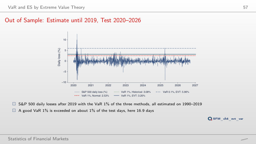
                                                                  Out of Sample: Estimate until 2019, Test 2020–2026
                                                                  Slide 57: Out of Sample: Estimate until 2019, Test 2020–2026
                                                                  Slide 57
                                                                    Question for the room For the S&P 500, the VaR 1% of the Normal distribution is exceeded on 44 days of 2020–2026, against 16.9 expected. The ▶ button goes through the four series. How many times is the Normal VaR 1% of BET exceeded, where 16.8 exceedances are expected?
                                                                    Answer

                                                                    13 times, below the expected value; the EVT VaR 4 times, the historical one 5 times. The test period was calmer for BET than the estimation period 1997–2019. A VaR estimated once does not follow the volatility: there are too many exceedances after 2020 for the S&P 500 (EVT 25, historical 26) and too few for BET. At VaR 0.1%, the Normal distribution is still exceeded too often for all four series: S&P 500 23 days against 1.7, BET 4 against 1.7, Bitcoin 8 against 2.5.

                                                                    Counting the Exceedances
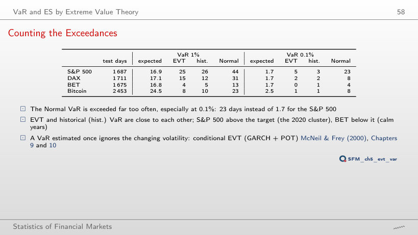
                                                                    Slide 58: Counting the Exceedances
                                                                    Slide 58

                                                                    Worked example: the Kupiec test

                                                                    \[\begin{gathered}\mathrm{LR} = -2\ln\big[(1 - p)^{n - x} p^{x}\big] + 2\ln\big[(1 - \hat\pi)^{n - x}\hat\pi^{x}\big], \qquad \hat\pi = \frac{x}{n},\\ \mathrm{LR} \sim \chi^2_1: \;\text{rejected at 5}\%\text{ if}\; \mathrm{LR} > 3.84\end{gathered}\]
                                                                        Question for the room BET: the EVT VaR 1%, estimated until 2019, is exceeded on 4 of the 1,675 test days, against 16.8 expected. What does the Kupiec test say at 5%?
                                                                        Answer

                                                                        It rejects correct coverage: LR = 14.14, p-value 0.0002. The test is two-sided: too few exceedances mean a VaR too high for the test period, which was calmer for BET than the years 1997–2019. The Normal VaR of BET, with 13 exceedances, is not rejected (p-value 0.34), although at 0.1% it has 4 exceedances against 1.7. For the S&P 500, EVT (25 exceedances) is not rejected (p-value 0.063), historical simulation (26) is rejected (0.038), and the Normal distribution (44) has a p-value of 3 × 10⁻⁸.

                                                                        Daily losses L = −r, in %, from log returns: S&P 500 and DAX from January 1990, BET from September 1997, Bitcoin from September 2014 (7 days a week), to 18 September 2026; OMV Petrom, BRD, Banca Transilvania and Transgaz from 2010, from the adjusted price. EODHD closing prices. The GEV fits, the bootstrap intervals and the simulated maxima are those of the lecture (the same rules and the same generator seed); Hill, GPD, VaR and ES are recomputed in the browser from the same losses.