

Statistics of Financial Markets

Chapter 9 · ARCH and GARCH Models

The slide of the lecture is on the left, the same figure or table on the right, computed in the browser from the same data. The ▶ button moves the parameter step by step; the tables and worked examples are recomputed with it. Abbreviations: ARCH (autoregressive conditional heteroskedasticity), GARCH (generalised ARCH), GJR (Glosten–Jagannathan–Runkle), EGARCH (exponential GARCH), IGARCH (integrated GARCH), EWMA (exponentially weighted moving average), SE (standard error), LR (likelihood ratio), AIC and BIC (Akaike and Bayesian information criteria), ACF (autocorrelation function), ARCH-LM (Lagrange multiplier test for ARCH effects), QLIKE (quasi-likelihood), DM (Diebold–Mariano), VaR (value at risk).

Volatility Comes in Episodes · Conditional Mean and Conditional Variance · The ARCH Model · The GARCH(1,1) Model · Estimation by Maximum Likelihood · Heavy-Tailed Innovations · GARCH in Six Markets · Asymmetry and the Leverage Effect · Diagnostics · Model Selection · Forecasting Volatility · VaR 1% from a GARCH Model

Volatility Comes in Episodes

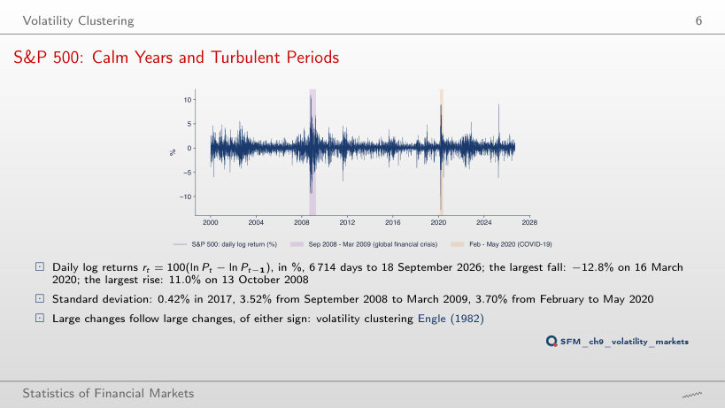
S&P 500: Calm Years and Turbulent Periods
Slide 6: S&P 500: Calm Years and Turbulent Periods
Slide 6
    Question for the room The daily standard deviation of the S&P 500 was 0.42% in 2017. How many times larger was it from September 2008 to March 2009?
    Answer

    8.3 times: 3.52/0.422 = 8.34; from February to May 2020, 3.70/0.422 = 8.76. The whole-sample standard deviation, 1.21%, averages calm and stormy days and describes neither regime: the 2008 episode is 2.9 times above it.

    Conditional Mean and Conditional Variance

    Worked Example: Conditional and Unconditional Variance
    Slide 12: Worked Example: Conditional and Unconditional Variance
    Slide 12

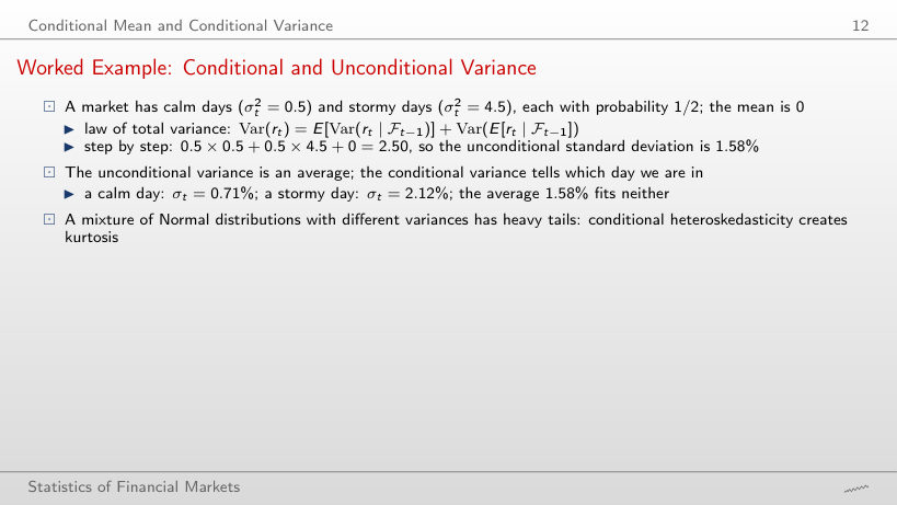
    Worked example: the law of total variance

    \[\mathrm{Var}(r_t) = E[\mathrm{Var}(r_t \mid \mathcal{F}_{t-1})] + \mathrm{Var}(E[r_t \mid \mathcal{F}_{t-1}]), \qquad K = \frac{3\,E[\sigma_t^4]}{(E[\sigma_t^2])^2}\]
        Question for the room Calm days with σ² = 0.5 and stormy days with σ² = 4.5, each with probability 1/2, mean 0. What is the unconditional standard deviation?
        Answer

        1.58%: the unconditional variance is the average of the variances, 0.5 × 0.5 + 0.5 × 4.5 = 2.50, and √2.50 = 1.58. The average of the volatilities, (0.71 + 2.12)/2 = 1.41%, is smaller, because the square root is concave. The mixture has kurtosis 4.92, although each regime is Normal.

        The ARCH Model

        ARCH(1): Properties
        Slide 15: ARCH(1): Properties
        Slide 15

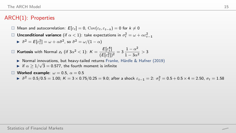
        Worked example: unconditional variance, kurtosis and one ARCH(1) step

        \[\bar\sigma^2 = \frac{\omega}{1-\alpha}, \qquad K = 3\,\frac{1-\alpha^2}{1-3\alpha^2}, \qquad \sigma_t^2 = \omega + \alpha\,\varepsilon_{t-1}^2\]
            Question for the room ARCH(1) with ω = 0.5: for α = 0.5 the kurtosis is 9.0. What happens to the kurtosis when ▶ takes α to 0.6?
            Answer

            It becomes infinite: 3α² = 1.08 ≥ 1, that is α exceeds 1/√3 = 0.577 and the fourth moment no longer exists. The unconditional variance stays finite, ω/(1 − α) = 0.5/0.4 = 1.25.

            Simulated Paths: i.i.d., ARCH(1) and GARCH(1,1)
            Slide 16: Simulated Paths: i.i.d., ARCH(1) and GARCH(1,1)
            Slide 16
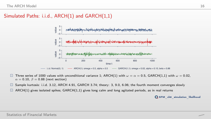
              Question for the room For ARCH(1) with ω = α = 0.5 the theoretical kurtosis is 9.0. What kurtosis does the simulated series of 1000 values have?
              Answer

              4.91, far below 9.0: the fourth moment converges slowly, because it depends on a few rare spikes. The i.i.d. series has 3.12 (theory 3), GARCH(1,1) has 3.74 (theory 6.06). With other seeds of the generator the sample values change a lot.

              ARCH(q) and Its Limits
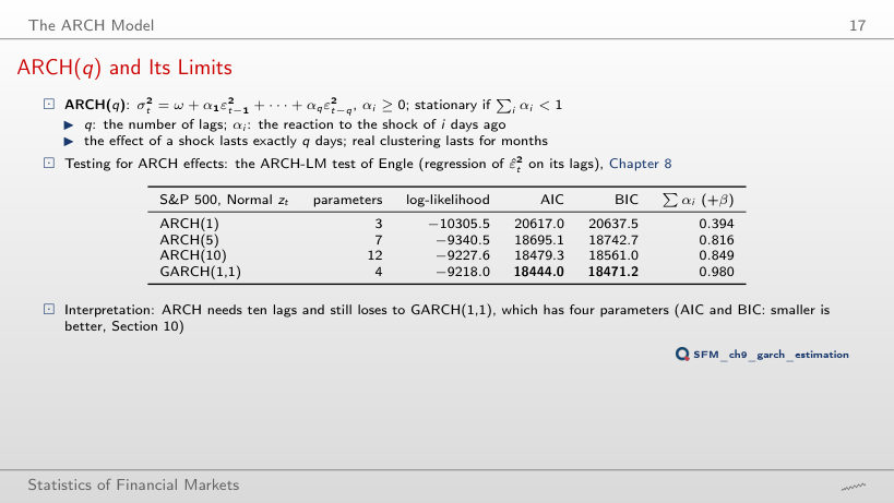
              Slide 17: ARCH(q) and Its Limits
              Slide 17

              Models with Normal innovations (in green: the smallest AIC and BIC)

                Question for the room S&P 500: ARCH(10) has 12 parameters and log-likelihood −9,227.6; GARCH(1,1) has 4 parameters and −9,218.0. Which model does BIC prefer?
                Answer

                GARCH(1,1): BIC 18,471.2 against 18,561.0 for ARCH(10), 89.8 lower. It has a higher likelihood with a third of the parameters: the term βσ²(t − 1) summarises all past shocks with geometric weights. The BIC of ARCH(q) falls with every added lag up to q = 10, but stays above that of GARCH(1,1).

                The GARCH(1,1) Model

                Stationarity, Long-Run Variance and Kurtosis
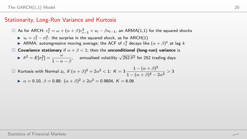
                Slide 20: Stationarity, Long-Run Variance and Kurtosis
                Slide 20

                Worked example: long-run variance and kurtosis

                \[\bar\sigma^2 = \frac{\omega}{1-\alpha-\beta}, \qquad K = 3\,\frac{1-(\alpha+\beta)^2}{1-(\alpha+\beta)^2-2\alpha^2}\]
                    Question for the room α = 0.10 and β = 0.88 give kurtosis 6.06. What does the kurtosis become when ▶ takes β to 0.89?
                    Answer

                    Infinite: (α + β)² + 2α² = 0.9801 + 0.02 = 1.0001 ≥ 1. The unconditional variance stays finite (α + β = 0.99 < 1; with ω = 0.02, σ̄² = 2.00), but the fourth moment no longer exists: the condition for the kurtosis is stricter than that for stationarity.

                    Persistence and Half-Life
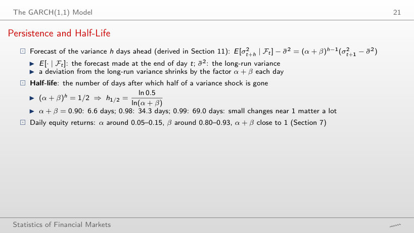
                    Slide 21: Persistence and Half-Life
                    Slide 21

                    Worked example: the half-life

                    \[(\alpha+\beta)^{h} = \tfrac12 \;\Rightarrow\; h_{1/2} = \frac{\ln 0.5}{\ln(\alpha+\beta)} \approx \frac{\ln 2}{1-\alpha-\beta}\]
                        Question for the room For α + β = 0.98 the half-life is 34.3 days. What is it for α + β = 0.99?
                        Answer

                        69.0 days, almost double: h½ ≈ ln 2/(1 − α − β), and 1 − α − β halves, from 0.02 to 0.01. For 0.90 it is 6.6 days; for the S&P 500 (α + β = 0.9947), 131 days.

                        Worked Example: One GARCH(1,1) Step
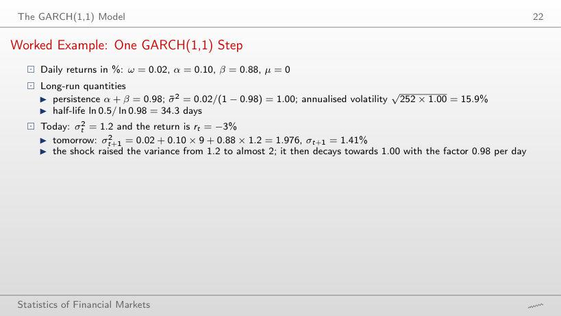
                        Slide 22: Worked Example: One GARCH(1,1) Step
                        Slide 22

                        Worked example: one GARCH(1,1) step

                        \[\sigma_{t+1}^2 = \omega + \alpha\,\varepsilon_t^2 + \beta\,\sigma_t^2, \qquad \varepsilon_t = r_t - \mu\]
                            Question for the room With σ²(t) = 1.2 and r(t) = −3%, σ²(t + 1) = 1.976. What is σ²(t + 1) after r(t) = +3%?
                            Answer

                            Also 1.976: GARCH(1,1) uses ε², so the sign of the shock does not matter (here μ = 0). The value 1.376 = 0.02 + 0.10 × 3 + 0.88 × 1.2 forgets the square. Asymmetry needs GJR-GARCH or EGARCH (Section 8).

                            IGARCH and the EWMA Link
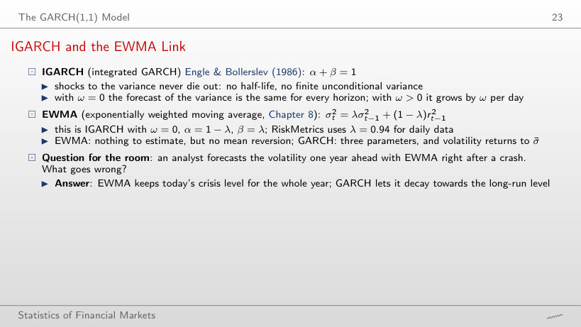
                            Slide 23: IGARCH and the EWMA Link
                            Slide 23

                            Worked example: IGARCH and GARCH forecasts after a crash

                            \[\alpha+\beta = 1: \quad E_t[\sigma_{t+h}^2] = \sigma_{t+1}^2 + (h-1)\,\omega; \qquad \alpha+\beta < 1: \quad E_t[\sigma_{t+h}^2] = \bar\sigma^2 + (\alpha+\beta)^{h-1}(\sigma_{t+1}^2 - \bar\sigma^2)\]
                                Question for the room An analyst forecasts the volatility one year ahead with EWMA right after a crash. What goes wrong?
                                Answer

                                EWMA keeps the crisis level for the whole year. S&P 500, at the close of 16 March 2020: EWMA (λ = 0.94) forecasts 84.0% a year for every horizon; GARCH(1,1)-t starts at 111.0% and falls to 62.0% after 250 days, towards the long-run level of 27.3%. EWMA is an IGARCH with ω = 0: no mean reversion.

                                Estimation by Maximum Likelihood

                                The Likelihood of ARCH(1)
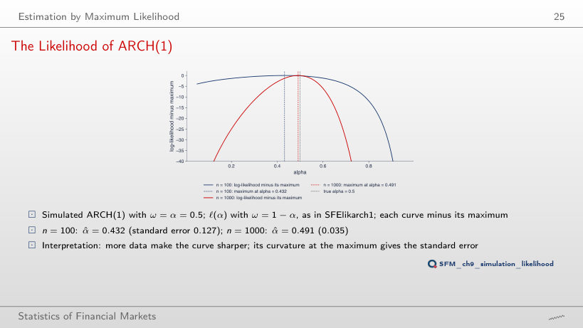
                                Slide 25: The Likelihood of ARCH(1)
                                Slide 25
                                  Question for the room With n = 100, α̂ = 0.432 and the standard error is 0.127. How does the standard error change with n = 1000?
                                  Answer

                                  It falls to 0.035, 3.6 times smaller; the √n rule gives √10 = 3.16. The log-likelihood curve gets sharper, and α̂ = 0.491 is closer to the true value 0.5.

                                  The Likelihood of GARCH(1,1)
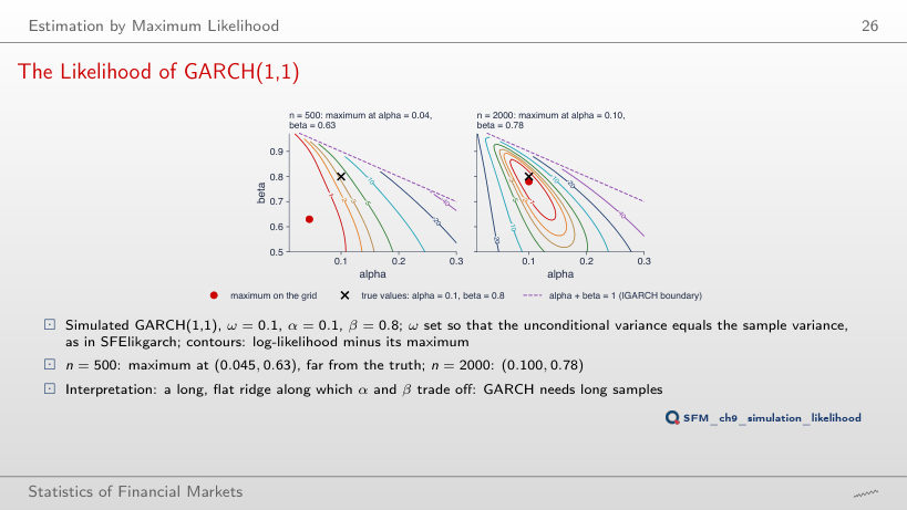
                                  Slide 26: The Likelihood of GARCH(1,1)
                                  Slide 26
                                    Question for the room With n = 500 the maximum on the grid is at (0.045, 0.63), far from the true values (0.1, 0.8). Where is the maximum with n = 2000?
                                    Answer

                                    At (0.100, 0.78), close to the true values: the long ridge along which α and β trade off narrows as n grows. With other seeds of the generator (extra runs) the maximum for n = 500 ranges from (0.025, 0.95) to (0.205, 0.67).

                                    Estimation Step by Step and with a Package
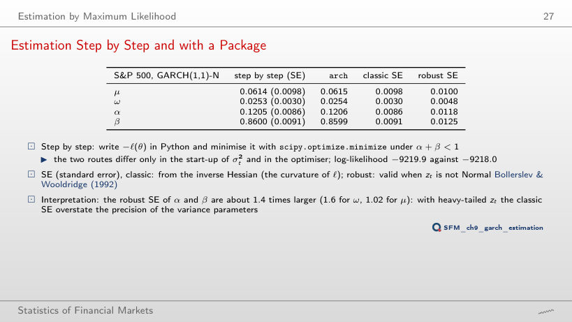
                                    Slide 27: Estimation Step by Step and with a Package
                                    Slide 27

                                    GARCH(1,1) with Normal innovations: step by step (scipy) and with the arch package

                                      Question for the room S&P 500, GARCH(1,1) with Normal innovations: the classic SE of α̂ is 0.0086. What is the robust SE?
                                      Answer

                                      0.0118, 1.37 times larger (β: 1.37; ω: 1.63; μ: 1.02). The innovations have heavy tails, and the classic SE, computed as if z(t) were Normal, overstate the precision of the variance parameters. For the BET the ratio exceeds 2.6.

                                      Heavy-Tailed Innovations

                                      S&P 500: Three Innovation Distributions
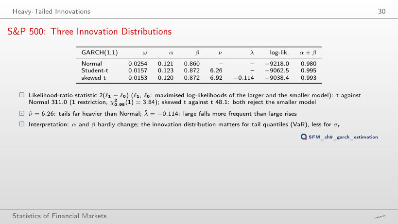
                                      Slide 30: S&P 500: Three Innovation Distributions
                                      Slide 30

                                      GARCH(1,1) with three innovation distributions

                                        Question for the room Moving from Normal to Student-t innovations raises the S&P 500 log-likelihood from −9,218.0 to −9,062.5. Do α and β change much?
                                        Answer

                                        Little: α from 0.121 to 0.123, β from 0.860 to 0.872; the persistence rises from 0.980 to 0.995. The LR statistic, 311.0, is far above 3.84: the innovation distribution matters for the tail quantiles (VaR) more than for σ(t).

                                        QQ Plots of the Standardised Residuals
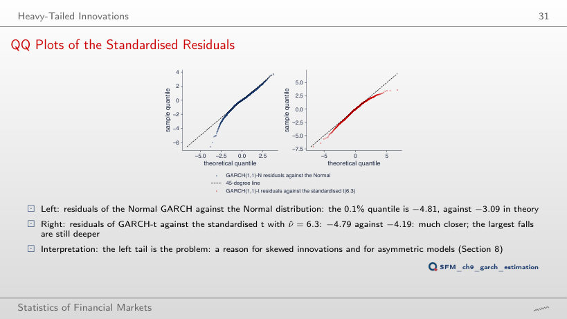
                                        Slide 31: QQ Plots of the Standardised Residuals
                                        Slide 31
                                          Question for the room The 0.1% quantile of the GARCH-N residuals is −4.81, against −3.09 for the Normal distribution. What is the 0.1% quantile of the standardised t with ν̂ = 6.26?
                                          Answer

                                          −4.19 = t⁻¹(0.001) × √((ν − 2)/ν) = −5.08 × 0.825. The GARCH-t residuals have −4.79: the t tail is much closer, but the largest falls are still deeper.

                                          GARCH in Six Markets

                                          GARCH(1,1)-t Estimates
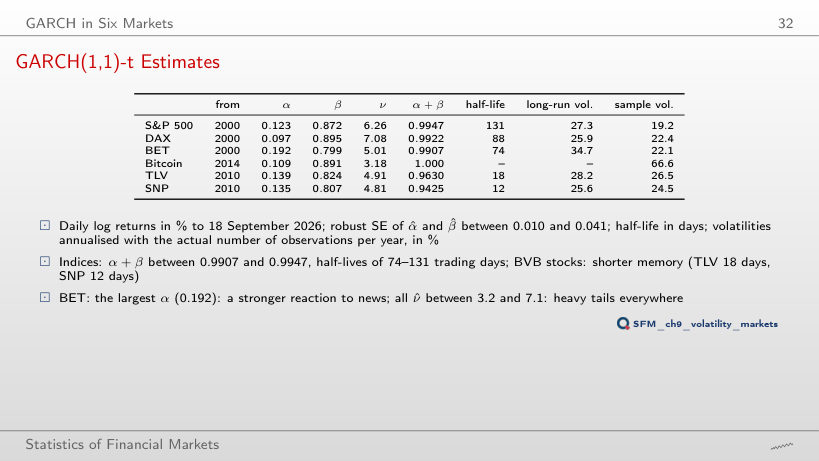
                                          Slide 32: GARCH(1,1)-t Estimates
                                          Slide 32

                                          GARCH(1,1) in six markets (robust SE; annualised volatilities, in %)

                                            Question for the room The BET has the largest α̂ of the six series (0.192). What does it mean?
                                            Answer

                                            A stronger reaction to yesterday's news: a 2% shock adds 0.192 × 4 = 0.77 to tomorrow's variance, against 0.123 × 4 = 0.49 for the S&P 500. The persistence is close, though (0.9907 against 0.9947), because the β̂ of the BET is smaller (0.799).

                                            Interpretation: Bitcoin and the Long-Run Volatility
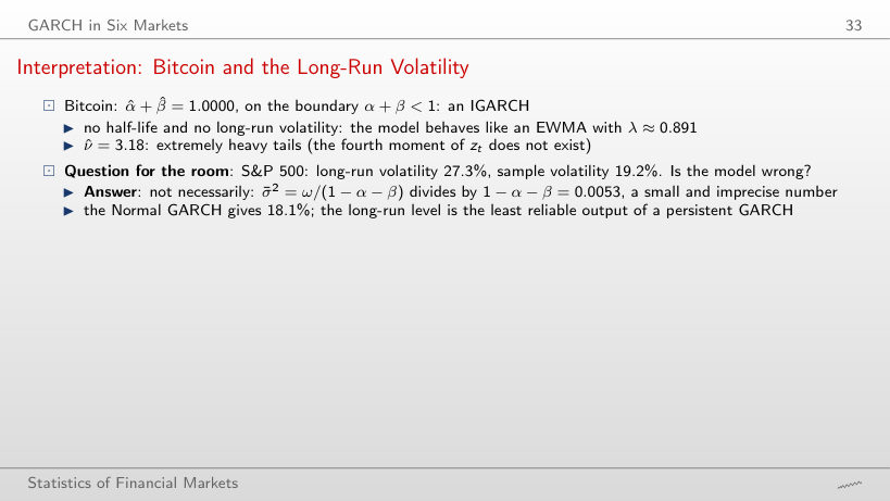
                                            Slide 33: Interpretation: Bitcoin and the Long-Run Volatility
                                            Slide 33

                                            Worked example: the long-run volatility

                                            \[\bar\sigma^2 = \frac{\omega}{1-\alpha-\beta}, \qquad \bar\sigma_{\text{year}} = \sqrt{A\,\bar\sigma^2}\]
                                                Question for the room S&P 500: long-run volatility 27.3%, sample volatility 19.2%. Is the model wrong?
                                                Answer

                                                Not necessarily: σ̄² = ω/(1 − α − β) divides by 1 − α − β = 0.0053, a small and imprecise number. With α + β lower by 0.002 (0.9927) the long-run volatility would be 23.3%; the Normal GARCH gives 18.1%. The long-run level is the least reliable output of a persistent GARCH.

                                                Conditional Volatility: S&P 500 and DAX
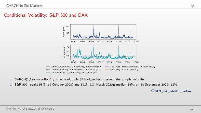
                                                Slide 34: Conditional Volatility: S&P 500 and DAX
                                                Slide 34
                                                  Question for the room The 2020 peak of the S&P 500 GARCH-t volatility is 111% a year (17 March 2020). What was the 2008 peak?
                                                  Answer

                                                  93%, on 16 October 2008: lower than in 2020, although the 2008 crisis lasted longer; the peak reflects the largest shocks of a short interval, not the length of the crisis. DAX: 80% in 2008 and 82% in 2020. The S&P 500 median is 14%, and the value on 18 September 2026 is 12%.

                                                  Conditional Volatility: BET and Bitcoin
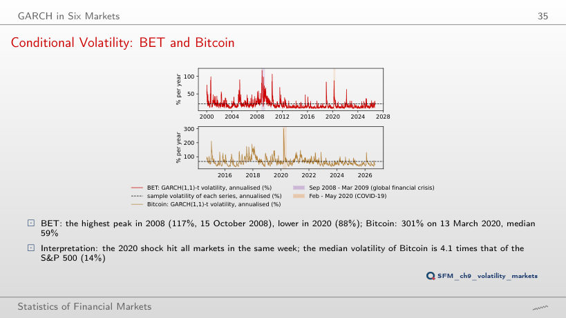
                                                  Slide 35: Conditional Volatility: BET and Bitcoin
                                                  Slide 35
                                                    Question for the room The median GARCH-t volatility of Bitcoin is 59% a year, that of the S&P 500 14%. How many times more volatile is Bitcoin?
                                                    Answer

                                                    4.1 times (58.7/14.3); the ratio of the variances would be 4.1² ≈ 17. Peaks: Bitcoin 301% on 13 March 2020, BET 117% on 15 October 2008 and 88% in March 2020.

                                                    Duration of a Volatility Shock
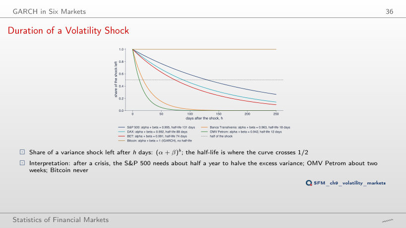
                                                    Slide 36: Duration of a Volatility Shock
                                                    Slide 36
                                                      Question for the room What is the half-life of a variance shock for Bitcoin?
                                                      Answer

                                                      There is none: α̂ + β̂ = 1.000 (IGARCH), so a shock does not die out. The S&P 500 needs 131 days, the DAX 88, the BET 74, TLV 18, SNP 12. With GJR-t the S&P 500 persistence (α + β + γ/2) is 0.983, a half-life of 41.5 days.

                                                      Asymmetry and the Leverage Effect

                                                      GJR-GARCH and EGARCH
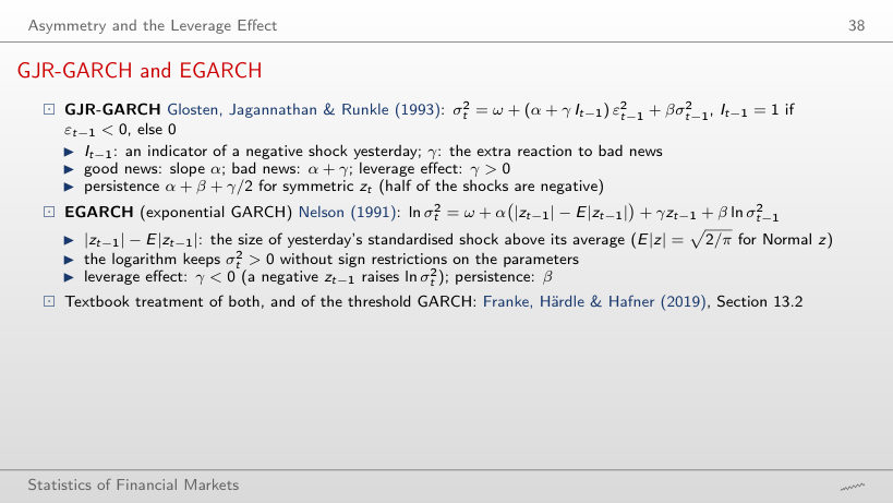
                                                      Slide 38: GJR-GARCH and EGARCH
                                                      Slide 38

                                                      Worked example: the impact of a fall and of a rise

                                                      \[\sigma_t^2 = \omega + (\alpha + \gamma\,I_{t-1})\,\varepsilon_{t-1}^2 + \beta\,\bar\sigma^2, \qquad I_{t-1} = 1 \text{ if } \varepsilon_{t-1} < 0\]
                                                          Question for the room S&P 500, GJR-t: α̂ = 0 and γ̂ = 0.205. By how much does a 2% rise raise tomorrow's variance, compared with a day without a shock?
                                                          Answer

                                                          By 0: good news has the slope α = 0. After a 2% fall the term (α + γ)ε² adds 0.205 × 4 = 0.821; with σ²(t − 1) fixed at the sample variance 1.471, tomorrow's variance is 2.136 after the fall and 1.315 after the rise: the ratio 1.62.

                                                          News Impact Curves: S&P 500 and Bitcoin
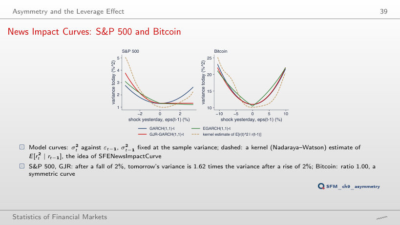
                                                          Slide 39: News Impact Curves: S&P 500 and Bitcoin
                                                          Slide 39
                                                            Question for the room S&P 500, GJR: the variance after a 2% fall is 1.62 times that after a 2% rise, with σ²(t − 1) equal to the sample variance. What happens to the ratio when ▶ raises σ²(t − 1) to 4 times the sample variance?
                                                            Answer

                                                            It falls to 1.16: the common term βσ²(t − 1) grows while the difference γε² stays the same, so it matters relatively less. With σ²(t − 1) at a quarter of the sample variance the ratio rises to 3.39: asymmetry shows most in calm periods.

                                                            Asymmetry in Six Markets
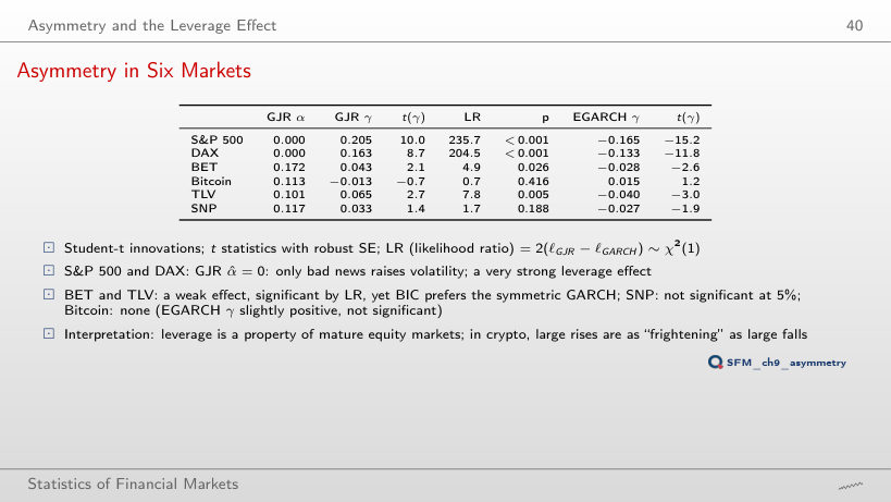
                                                            Slide 40: Asymmetry in Six Markets
                                                            Slide 40

                                                            GJR-GARCH(1,1) and EGARCH(1,1): the asymmetry parameter γ (t statistics with robust SE)

                                                              Question for the room BET: γ̂ = 0.043, t = 2.1, the LR test has p = 0.026, but BIC prefers the symmetric GARCH. Why?
                                                              Answer

                                                              BIC needs LR to exceed ln T = ln 6,670 = 8.8 for one more parameter; LR = 4.9 passes 3.84 (the 5% threshold) but not 8.8: the BET leverage effect is weak. For Bitcoin BIC picks EGARCH although γ is not significant: the logarithmic form fits the variance dynamics better, not the asymmetry.

                                                              Diagnostics

                                                              Autocorrelations Removed by GARCH
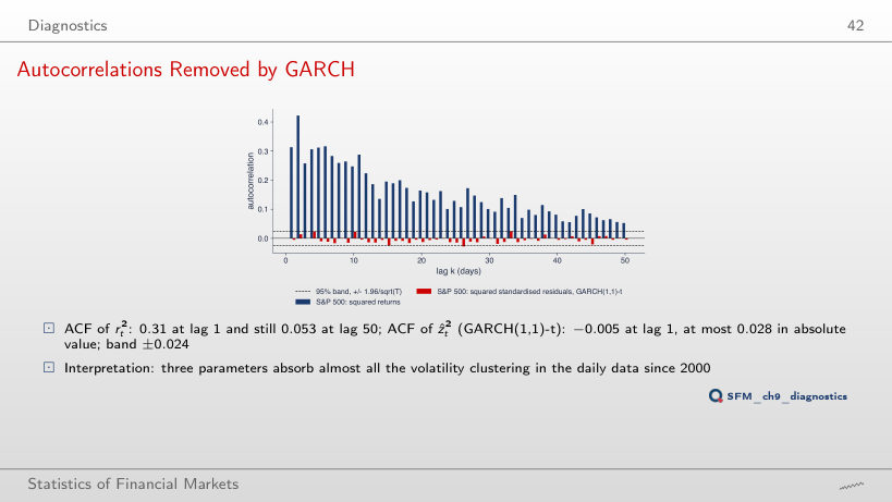
                                                              Slide 42: Autocorrelations Removed by GARCH
                                                              Slide 42
                                                                Question for the room The ACF of r² at lag 1 is 0.31. What is the ACF of ẑ² (GARCH-t) at lag 1?
                                                                Answer

                                                                −0.005, inside the band ±0.024; the largest absolute value over 50 lags is 0.028. Three variance parameters absorb almost all the volatility clustering; at lag 50 the ACF of r² is still 0.053.

                                                                Diagnostics on Real Data
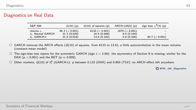
                                                                Slide 43: Diagnostics on Real Data
                                                                Slide 43

                                                                Tests on the returns and on the standardised residuals

                                                                  Question for the room S&P 500, GARCH-t: Q(10) on ẑ² has p = 0.192, and the sign-bias test has p < 0.001. Is the model correct?
                                                                  Answer

                                                                  Not entirely: no ARCH effects are left (Q(10) of the squares falls from 6,133 to 13.6), but the sign of past shocks still anticipates the variance (sign t = 3.56): the asymmetry is missing. A test that does not reject does not prove the model correct.

                                                                  Model Selection

                                                                  Nine Models for the S&P 500
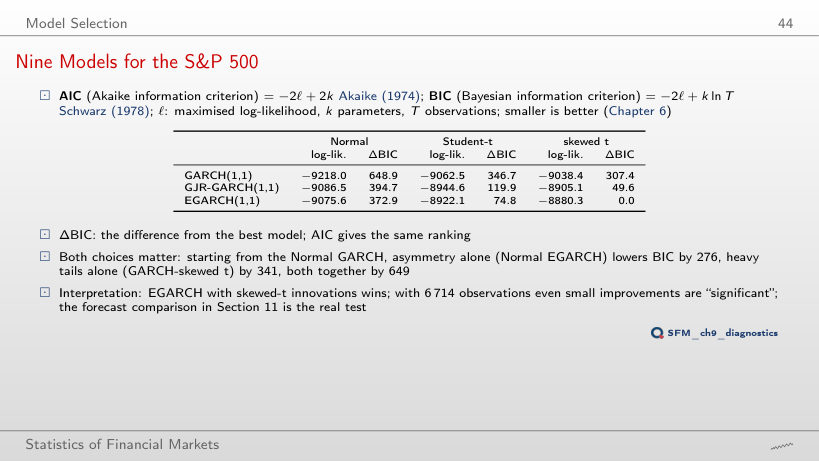
                                                                  Slide 44: Nine Models for the S&P 500
                                                                  Slide 44

                                                                  Log-likelihood and the difference from the best model (in green)

                                                                    Question for the room S&P 500, starting from GARCH with Normal innovations: which lowers BIC more, asymmetry (EGARCH with Normal innovations) or heavy tails (GARCH with skewed t)?
                                                                    Answer

                                                                    Heavy tails: 341, against 276 for asymmetry; both together (EGARCH with skewed t) lower BIC by 649, the best of the nine models. AIC gives the same order.

                                                                    Forecasting Volatility

                                                                    Worked Example: the S&P 500 on 18 September 2026
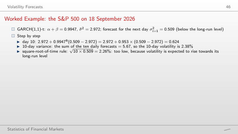
                                                                    Slide 46: Worked Example: the S&P 500 on 18 September 2026
                                                                    Slide 46

                                                                    Worked example: the H-day forecast

                                                                    \[E_t[\sigma_{t+h}^2] = \bar\sigma^2 + (\alpha+\beta)^{h-1}(\sigma_{t+1}^2 - \bar\sigma^2), \qquad \mathrm{Var}_t\Big(\sum_{h=1}^{H} r_{t+h}\Big) = \sum_{h=1}^{H} E_t[\sigma_{t+h}^2]\]
                                                                        Question for the room On 18 September 2026, σ²(t + 1) = 0.509, below σ̄² = 2.972. The square-root-of-time rule gives the 10-day volatility √(10 × 0.509) = 2.26%. What does the sum of the GARCH forecasts give?
                                                                        Answer

                                                                        2.38%: the daily forecasts rise towards the long-run level (day 10: 0.624), so their sum, 5.67, exceeds 10 × 0.509 = 5.09. In a crisis the relation reverses: the square-root rule gives values that are too large.

                                                                        The Term Structure of Volatility
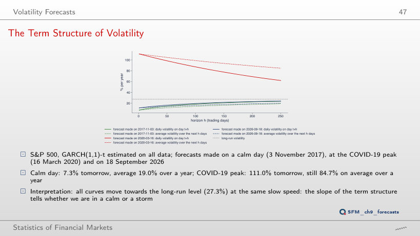
                                                                        Slide 47: The Term Structure of Volatility
                                                                        Slide 47
                                                                          Question for the room On 16 March 2020 the forecast for the next day is 111.0% a year. What is the forecast average volatility over the next 250 days?
                                                                          Answer

                                                                          84.7%: with α + β = 0.9947 the gap to the long-run level shrinks by only 0.53% a day, and after 250 days the daily forecast is still 62.0%. On a calm day (3 November 2017) the curve rises: 7.3% tomorrow, 19.0% on average over a year.

                                                                          GARCH against EWMA, Out of Sample
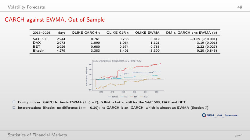
                                                                          Slide 49: GARCH against EWMA, Out of Sample
                                                                          Slide 49

                                                                          Next-day variance forecasts (in green: the smallest QLIKE; DM: t and p)

                                                                            Question for the room Bitcoin, 2015–2026: QLIKE GARCH-t 3.383, EWMA 3.390, DM test t = −0.20 (p = 0.845). What do you conclude?
                                                                            Answer

                                                                            No detectable difference: the Bitcoin GARCH is an IGARCH, that is almost an EWMA. A large p does not show that the forecasts are equal, only that the test does not separate them. For the S&P 500 (t = −3.69), the DAX (−3.19) and the BET (−2.22) GARCH-t is significantly better.

                                                                            VaR 1% from a GARCH Model

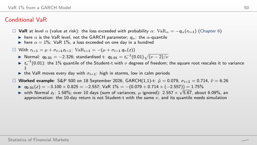
                                                                            Conditional VaR
                                                                            Slide 50: Conditional VaR
                                                                            Slide 50

                                                                            Worked example: one-day and H-day VaR

                                                                            \[\mathrm{VaR}_{t+1} = -\big(\mu + \sigma_{t+1}\,q_\alpha(z)\big), \qquad q_\alpha(z) = t_\nu^{-1}(\alpha)\sqrt{\tfrac{\nu-2}{\nu}}\]
                                                                                Question for the room S&P 500 on 18 September 2026: the one-day VaR 1% is 1.75%. The √10 rule gives over 10 days 1.75 × √10 = 5.52%. What does the sum of the variance forecasts give (with the t quantile and without μ)?
                                                                                Answer

                                                                                6.09% = 2.557 × √5.67: volatility is expected to rise towards its long-run level, so the √10 rule gives too little. This is an approximation: the 10-day return is not Student-t with the same ν, and its exact quantile needs simulation.

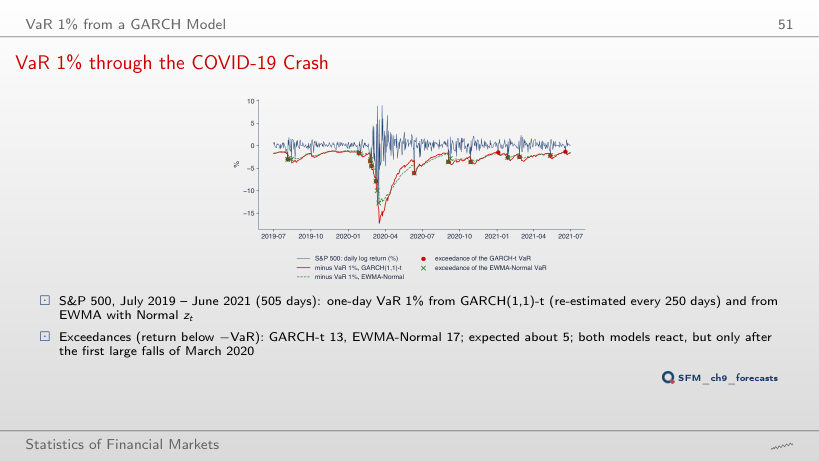
                                                                                VaR 1% through the COVID-19 Crash
                                                                                Slide 51: VaR 1% through the COVID-19 Crash
                                                                                Slide 51
                                                                                  Question for the room S&P 500, July 2019 – June 2021, 505 days: how many times is the GARCH-t VaR 1% exceeded?
                                                                                  Answer

                                                                                  13 times, against about 5 expected (1% of 505); EWMA-Normal is exceeded 17 times. Both models react, but only after the first large falls of March 2020: a one-day forecast cannot anticipate the first shock.

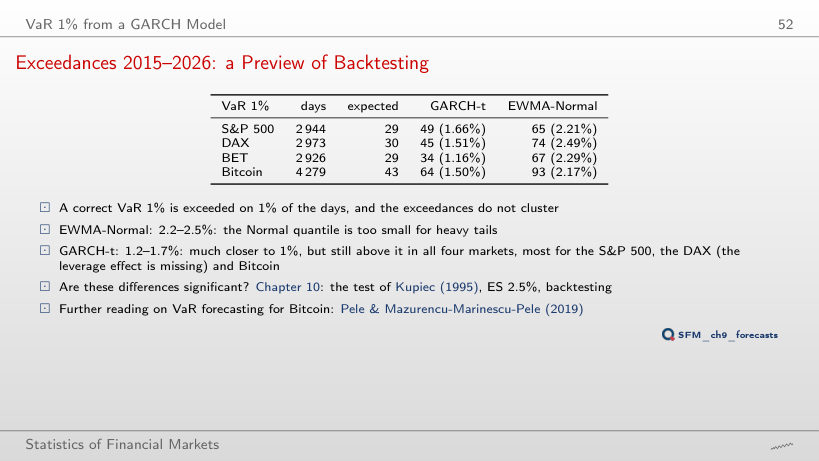
                                                                                  Exceedances 2015–2026: a Preview of Backtesting
                                                                                  Slide 52: Exceedances 2015–2026: a Preview of Backtesting
                                                                                  Slide 52

                                                                                  Exceedances of the one-day VaR, out of sample

                                                                                    Question for the room EWMA with Normal innovations exceeds the VaR 1% on 2.2–2.5% of the days in all four markets. Why?
                                                                                    Answer

                                                                                    The Normal quantile, −2.326, is not deep enough for heavy tails. GARCH-t, with the Student-t quantile, has 1.2–1.7%: much closer to 1%, but still above 1% in all four markets. Whether the differences are significant is tested in Chapter 10 (the Kupiec test).

                                                                                    Daily log returns, in %: S&P 500, DAX and BET from January 2000, Bitcoin from September 2014 (7 days a week), Banca Transilvania (TLV) and OMV Petrom (SNP) from 2010, from the adjusted price, to 18 September 2026; the two erroneous TLV days of May 2016 are removed. EODHD prices. The models are estimated with the arch package, with the code of the lecture (maximum likelihood, robust SE); from the fitted parameters the browser rebuilds the conditional variance day by day and computes from it the standardised residuals, the QQ plots, the news impact curves, the diagnostic tests, the information criteria, the forecasts and the VaR. The out-of-sample forecasts of GARCH-t and GJR-t (re-estimated every 250 days) are those of the lecture; the EWMA, the QLIKE losses, the DM tests and the exceedances are recomputed in the browser. The simulations use the Normal draws of the lecture's generator (the same seed). Other innovation distributions, other sample starts, other markets for the S&P 500 tables, ARCH(q) of other orders, other seeds and parameters of the simulations, other VaR levels and other evaluation periods are extra runs of the same code.