

Time Series Analysis

Chapter 3 · Unit Roots and ARIMA Models

The slide of the lecture is on the left, the same figure on the right, computed in the browser from the same data. The ▶ button moves the parameter step by step.

Deterministic and stochastic trends · Spurious regression · The Dickey–Fuller test · Phillips–Perron, KPSS and their joint use · Structural breaks · ARIMA(p,d,q) models · ARIMA in practice

Deterministic and stochastic trends

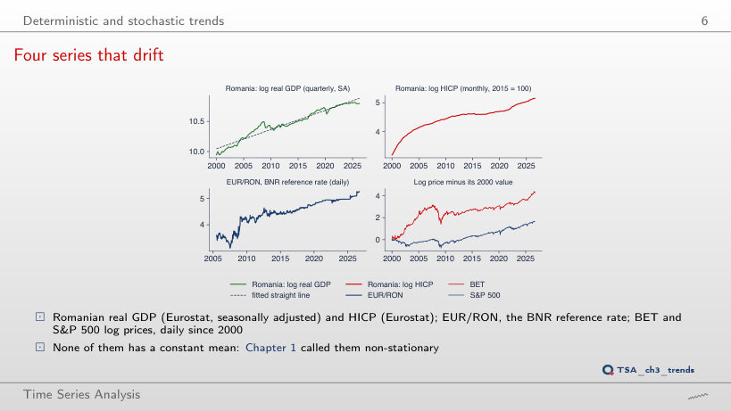
Four series that drift
Slide 6: Four series that drift
Slide 6
    Question for the room The ▶ button moves the end of the sample on which the dashed straight lines of all four panels are fitted. Where is GDP in 2026Q2 relative to a line fitted on the data up to 2008Q3?
    Answer

    Far below it: the line fitted up to 2008Q3 has a slope of 1.56% per quarter, and GDP in 2026Q2 is 76 log points (100 × the difference of logs) below its extension. On the full sample the slope is 0.80% per quarter (about 3.2% a year), and the largest deviation, 17.5 log points, occurs in 2008Q3. After the 2009 recession GDP did not return to the earlier line: an argument for a stochastic trend, not for a fixed line plus noise.

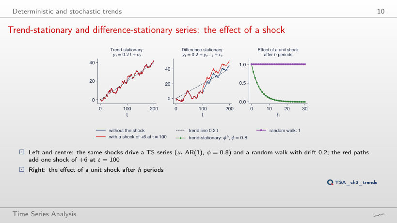
    Trend-stationary and difference-stationary series: the effect of a shock
    Slide 10: Trend-stationary and difference-stationary series: the effect of a shock
    Slide 10
      Question for the room The ▶ button raises φ from 0 to 1. What is left, at the end of the sample, of the +6 shock in the trend-stationary series?
      Answer

      For φ < 1, almost nothing: 6φ⁹⁹ is 1.5 · 10⁻⁹ at φ = 0.8 and 0.04 at φ = 0.95; only at φ = 0.99 does 2.2 remain. At φ = 1 the whole shock, 6, remains, as for the random walk: the AR(1) noise becomes a random walk itself, and the two models coincide. With φ = 0.8, the effect of a unit shock is 0.107 after 10 periods, and the half-life is 3.1 periods.

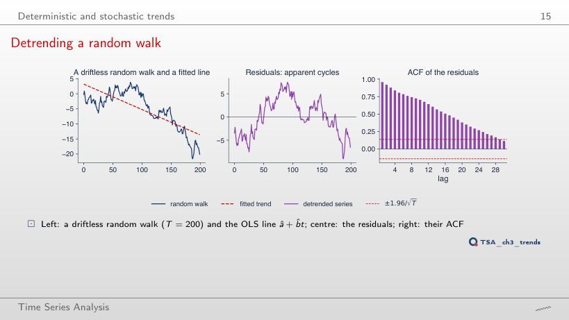
      Detrending a random walk
      Slide 15: Detrending a random walk
      Slide 15
        Question for the room The true slope of the random walk is 0. On 2,000 random walks with T = 200, how often does the t-test reject “the slope is 0” at 5%?
        Answer

        In 90.4% of the cases, not in 5%; the median R² is 0.44. On the path of the slide, R² = 0.61 and t = −17.7. The residuals have ρ̂(1) = 0.96 and stay positively autocorrelated up to lag 36: long cycles created by detrending (Nelson and Kang). With T = 50 the test still rejects in 82.0% of the cases: the error does not go away with a shorter or a longer sample.

        Spurious regression

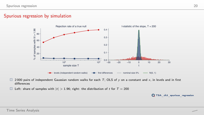
        Spurious regression by simulation
        Slide 20: Spurious regression by simulation
        Slide 20
          Question for the room In levels, the t-test rejects b = 0 in 83.6% of the samples for T = 200. What happens to the rejection rate when T rises to 1,000?
          Answer

          It rises, to 92.3%: the median |t| goes from 6.3 to 14.2, roughly like √T; the median R² stays around 0.17, and the median DW falls to 0.015. More data do not correct a spurious regression. In differences, the rate stays close to the nominal level: 4.65% at T = 200 and 4.5% at T = 1,000.

          A spurious regression on real data
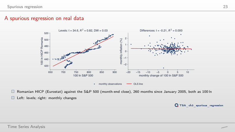
          Slide 23: A spurious regression on real data
          Slide 23
            Question for the room On 2005–2026, the regression of the HICP on the S&P 500 in levels gives t = 34.6 and R² = 0.82. Does the relation remain if we use only 2005–2012?
            Answer

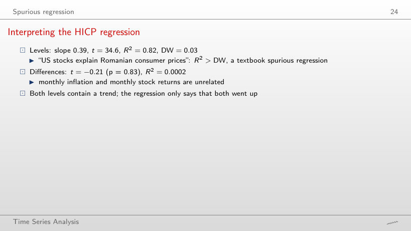
            No: on 2005–2012, t = −0.72 and R² is below 0.01 in levels; on 2013–2026, t = 33.2 and R² = 0.87. In 2005–2012 stocks fell and recovered while prices rose; after 2013 both rise. In differences, on the full sample, t = −0.21 (p = 0.83) and R² = 0.0002. The Granger–Newbold rule flags the problem: R² = 0.82 > DW = 0.03.

            Interpreting the HICP regression
            Slide 24: Interpreting the HICP regression
            Slide 24

            Worked example

            \[\hat b=\frac{\sum_t(x_t-\bar x)(y_t-\bar y)}{\sum_t(x_t-\bar x)^2},\quad t=\frac{\hat b}{\sqrt{s^2/\sum_t(x_t-\bar x)^2}},\quad R^2=\frac{t^2}{t^2+n-2},\quad \mathrm{DW}=\frac{\sum_t(e_t-e_{t-1})^2}{\sum_t e_t^2}\]
                Question for the room In levels, the regression of the HICP on the S&P 500 has t = 34.6 and R² = 0.82. Is R² new information beyond t?
                Answer

                No: with one regressor, R² = t²/(t² + n − 2) = 34.6²/(34.6² + 258) = 0.82. Both come from the same standard error, which is far too small because the error is itself a random walk; DW = 0.03 shows it. In monthly differences, t = −0.21 (p = 0.83) and R² = 0.0002: monthly inflation and stock returns are unrelated.

                The Dickey–Fuller test

                The Dickey–Fuller distributions
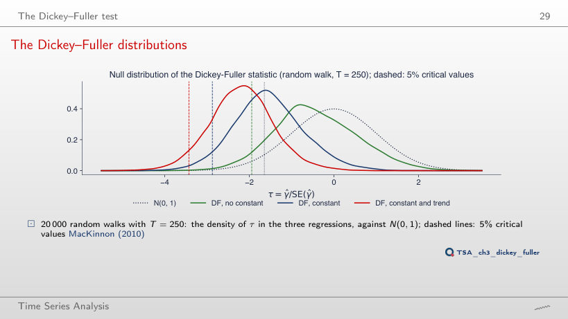
                Slide 29: The Dickey–Fuller distributions
                Slide 29
                  Question for the room If we use the critical value of the Normal distribution, −1.645, how often do we “reject” a true unit root in the regression with constant and trend?
                  Answer

                  In 77.4% of the samples (46.1% with a constant, 9.8% without a constant), against 5% under N(0, 1). To reject in 5% of the cases, the critical value must move down to the 5% quantile of the Dickey–Fuller distribution: −1.95, −2.86 and −3.42 in the simulation; −1.94, −2.87 and −3.43 in the MacKinnon tables. With −3.42, the share for constant and trend is 4.99%.

                  Critical values of the Dickey–Fuller test
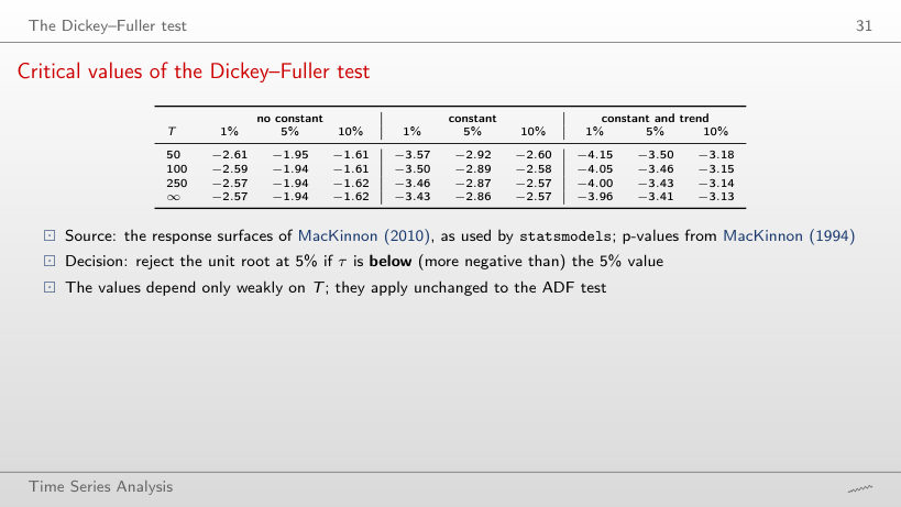
                  Slide 31: Critical values of the Dickey–Fuller test
                  Slide 31
                    Question for the room With T = 50 and a regression with a constant, τ = −2.90. Do we reject the unit root at 5%?
                    Answer

                    No: the 5% critical value for T = 50 is −2.92, and −2.90 > −2.92. With the asymptotic value −2.86 we would have rejected it: the critical values depend only weakly on T, but it matters when τ is close to the threshold. With the Normal value −1.645 the rejection would have been "clear" and wrong.

                    Worked example: Romanian real GDP
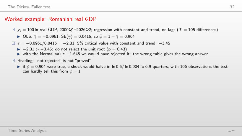
                    Slide 32: Worked example: Romanian real GDP
                    Slide 32

                    Worked example

                    \[\Delta y_t=c+bt+\gamma y_{t-1}+\sum_{j=1}^{k}\delta_j\Delta y_{t-j}+\varepsilon_t,\qquad \tau=\frac{\hat\gamma}{\mathrm{SE}(\hat\gamma)},\qquad \hat\phi=1+\hat\gamma\]
                        Question for the room What happens to τ for GDP if we drop the trend from the regression (constant only, k = 0)?
                        Answer

                        τ becomes −1.80 (γ̂ = −0.0173, SE 0.0096), with critical value −2.89 and p = 0.38: still no rejection. Without a constant, τ = 3.29 and p ≈ 1. For a trending series the right alternative is the one with a trend: the slide has τ = −2.31 against −3.45 (p = 0.43). Here the conclusion does not depend on the deterministic terms, but the critical value changes with each case.

                        Choosing the number of lags k
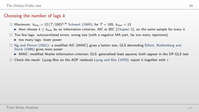
                        Slide 34: Choosing the number of lags k
                        Slide 34

                        Worked example

                        \[k_{\max}=\Big\lceil 12\Big(\frac{T}{100}\Big)^{1/4}\Big\rceil,\qquad \mathrm{AIC}=-2\ln L+2m,\qquad \mathrm{BIC}=-2\ln L+m\ln N\]
                            Question for the room For the HICP (100 ln P), AIC chooses k = 6. What does BIC choose, and does the conclusion change?
                            Answer

                            BIC chooses k = 1, because it penalises each lag by ln N instead of 2: τ = −0.38 (p = 0.988), against τ = −0.96 (p = 0.949) with k = 6. The conclusion is the same: the unit root is not rejected. The lags change τ, which is why k is reported together with τ.

                            Size and power of the Dickey–Fuller test
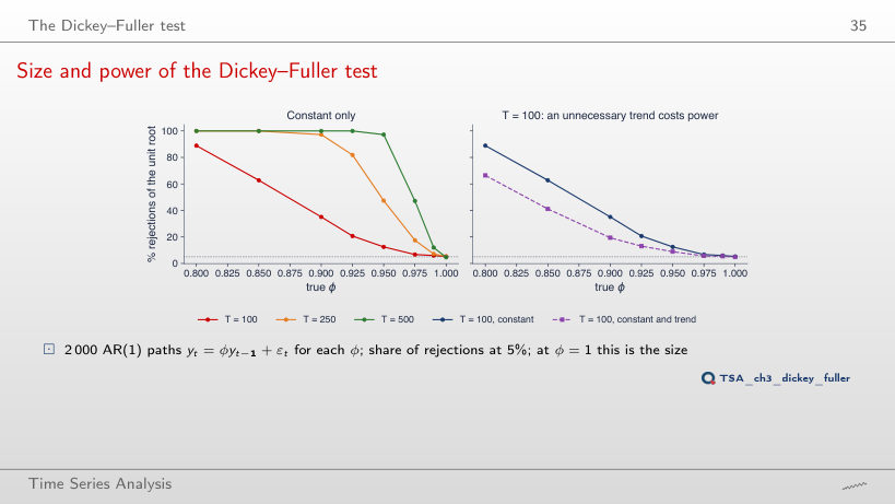
                            Slide 35: Size and power of the Dickey–Fuller test
                            Slide 35
                              Question for the room With a quarterly series of 25 years (T = 100) and φ = 0.95, how often does the Dickey–Fuller test with a constant reject the unit root at 5%?
                              Answer

                              In 12.5% of the cases: the test almost never tells φ = 0.95 from φ = 1. With T = 250, 47.4%; with T = 500, 97.25%. At φ = 1 the shares are the size of the test: 5.3%, 5.2% and 4.65% with a constant. An unnecessary trend costs power: at T = 100 and φ = 0.9, 35.1% with a constant and 19.4% with constant and trend.

                              Interpreting the power curves
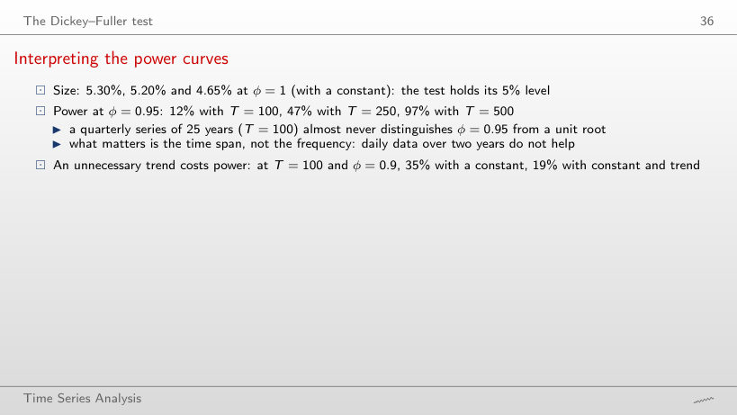
                              Slide 36: Interpreting the power curves
                              Slide 36
                                Question for the room With T = 100 quarters (25 years) and φ = 0.95, how often does the DF test (constant) reject the unit root?
                                Answer

                                In 12.5% of the cases; with constant and trend, in 8.9%. To reach 97.3% it needs T = 500. At φ = 1 the test rejects in 5.3%, 5.2% and 4.65% of the cases (T = 100, 250, 500): the size is right, the power in short samples is low.

                                Phillips–Perron, KPSS and their joint use

                                The KPSS test: stationarity as the null
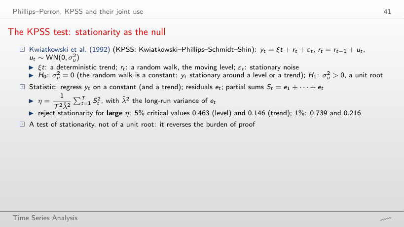
                                Slide 41: The KPSS test: stationarity as the null
                                Slide 41

                                Worked example

                                \[S_t=\sum_{s\le t}e_s,\qquad \hat\lambda^2=\hat\gamma_0+2\sum_{j=1}^{L}\Big(1-\frac{j}{L+1}\Big)\hat\gamma_j,\qquad \eta=\frac{\sum_{t=1}^{T}S_t^2}{T^2\hat\lambda^2}\]
                                    Question for the room For Romanian GDP, η = 0.198 around a trend. What is η around a level, and why?
                                    Answer

                                    η = 1.533 (L = 6), far above 0.463. Around a constant, the residuals contain the whole trend: negative at the start and positive at the end, and the partial sums make huge excursions. A trending series needs the trend version, with critical value 0.146; there 0.198 > 0.146 rejects stationarity at 5%, but not at 1% (0.216).

                                    KPSS: why partial sums
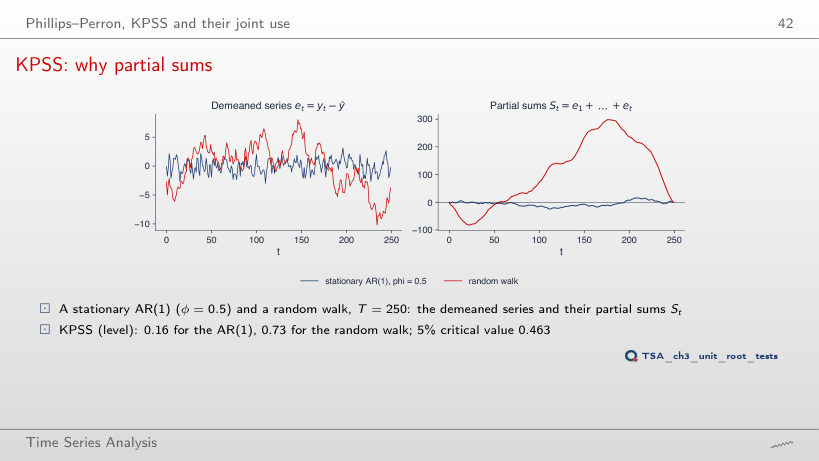
                                    Slide 42: KPSS: why partial sums
                                    Slide 42
                                      Question for the room The ▶ button raises φ of the AR(1) series from 0 to 1. From which value does KPSS reject stationarity at 5%?
                                      Answer

                                      Only from φ = 0.95: KPSS = 0.565 > 0.463 (p = 0.027). At φ = 0.9 the statistic is 0.326 and the test does not reject, although the series is very persistent; at φ = 1 it rises to 1.213. For the random walk of the panel, KPSS = 0.733 (p = 0.011). The partial sums of a persistent series wander far from 0, and η grows.

                                      ADF and KPSS together
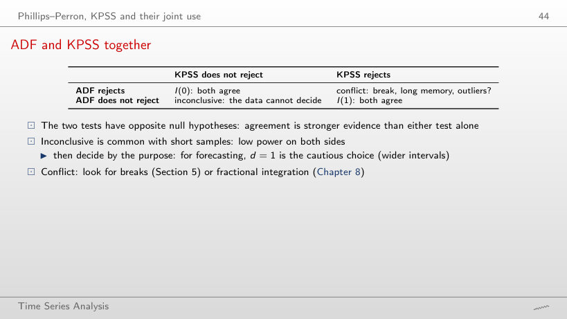
                                      Slide 44: ADF and KPSS together
                                      Slide 44
                                        Question for the room At 1% instead of 5%, in which cell does Romanian GDP land?
                                        Answer

                                        In "inconclusive": ADF still does not reject (p = 0.43), and KPSS = 0.198 is below the 1% critical value, 0.216. At 10%, 12-month inflation moves to I(1) (KPSS 0.404 > 0.347), and the BET and S&P 500 returns and US GDP growth move to "conflict": at the 10% level KPSS rejects more easily.

                                        Unit-root tests on real series
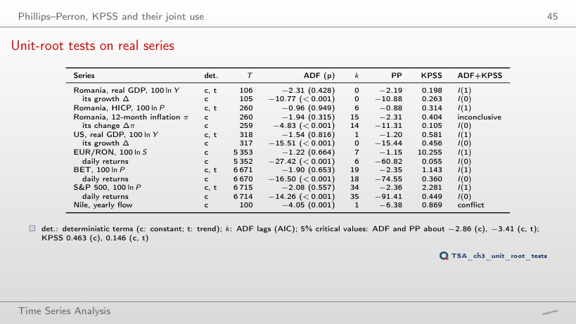
                                        Slide 45: Unit-root tests on real series
                                        Slide 45
                                          Question for the room If every series is tested with constant and trend, what happens to 12-month inflation?
                                          Answer

                                          It becomes I(1): KPSS around a trend is 0.399 > 0.146, while ADF still does not reject (τ = −1.99, p = 0.61). The BET returns move to "conflict" (KPSS 0.250 > 0.146). The verdict depends on the alternative chosen; for series without a trend, the constant is the choice of the lecture.

                                          Structural breaks

                                          A level shift misleads the ADF test
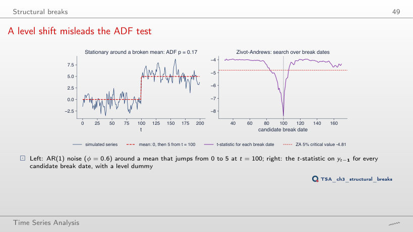
                                          Slide 49: A level shift misleads the ADF test
                                          Slide 49
                                            Question for the room The ▶ button raises the jump of the mean from 0 to 10. From which size of the jump does ADF stop rejecting the unit root at 5%, on this stationary series?
                                            Answer

                                            From a jump of 3.5 (p = 0.056); at 3, p = 0.030. At the jump of the lecture, 5, p = 0.17, and on 2,000 series with the same jump the DF test rejects in 71.5% of the cases (without the jump: 100%); at a jump of 7, only in 0.55%. Zivot–Andrews includes the break and rejects for every jump: at a jump of 5, ZA = −7.47 (one lag chosen by AIC), far below −4.81, with the level changing from t = 100. The curve on the right is computed without lags: its minimum, −8.37, is reached at t = 100; −7.47 is the test statistic, not the minimum of the curve.

                                            Interpreting the simulated break
                                            Slide 50: Interpreting the simulated break
                                            Slide 50
                                              Question for the room The slide gives ZA = −7.47 and says that the minimum is reached at t = 100. Is −7.47 the minimum of the curve in the previous chart?
                                              Answer

                                              No. The curve of the chart, without lags, has its minimum −8.37 at t = 100. The statsmodels Zivot–Andrews statistic chooses the lags by AIC (here 1 lag) and gives −7.47, with the break also at t = 100. Both are far below −4.81, so the conclusion does not change: the series is stationary around a mean with one break.

                                              Zivot–Andrews on two real series
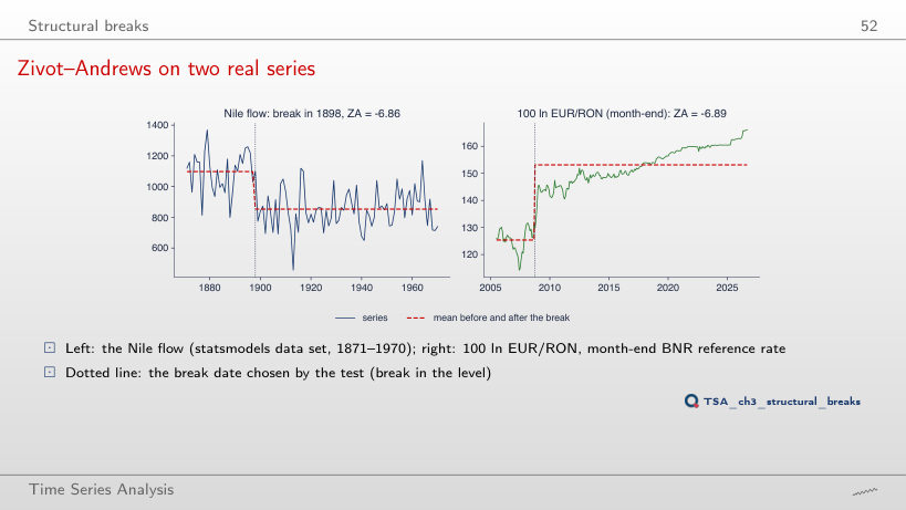
                                              Slide 52: Zivot–Andrews on two real series
                                              Slide 52
                                                Question for the room For EUR/RON, ZA with a break in the level gives −6.89. What does the variant with a break in the trend only give?
                                                Answer

                                                ZA = −4.40, with a 5% critical value of −4.41 (p = 0.051): the unit root is no longer rejected at 5%, and the chosen date moves to July 2009. With a break in the level and the trend: −6.83, below −5.07, in October 2008. For the Nile, all three variants reject (−6.86, −5.68, −6.84); the level breaks are dated 1898, the trend break 1914. The result depends on the assumed form of the break.

                                                Interpreting the two breaks
                                                Slide 53: Interpreting the two breaks
                                                Slide 53
                                                  Question for the room For EUR/RON, does Zivot–Andrews still reject if the break is allowed only in the trend?
                                                  Answer

                                                  Just not: ZA = −4.40 and the 5% critical value is −4.41 (p = 0.051), with the break in July 2009. With the break in the level (−6.89) or in both (−6.83, critical value −5.07) it rejects, with the break in October 2008. For the Nile all three versions reject.

                                                  ARIMA(p,d,q) models

                                                  Romanian GDP: identification
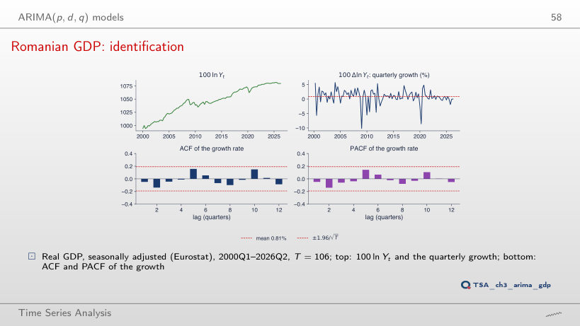
                                                  Slide 58: Romanian GDP: identification
                                                  Slide 58
                                                    Question for the room On the full sample, no autocorrelation of growth leaves the band. Does this still hold if the sample stops in 2008Q4, before the crisis?
                                                    Answer

                                                    Not entirely: with 35 growth rates (2000Q2–2008Q4), the mean is 1.57% per quarter, ρ̂(1) = −0.27, and one ACF value leaves the ±0.33 band; the Ljung–Box Q*(8) = 11.1 (p = 0.20) does not reject white noise, though. On the full sample: mean 0.81%, ρ̂(1) = −0.05, ρ̂(2) = −0.14, Q*(8) = 7.3 (p = 0.51); up to 2019Q4, Q*(8) = 4.2 (p = 0.84).

                                                    Model choice by AICc
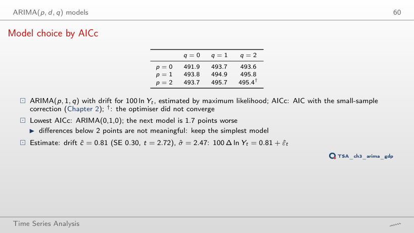
                                                    Slide 60: Model choice by AICc
                                                    Slide 60
                                                      Question for the room ARIMA(0,1,2) has an AICc 1.7 points higher. Is that evidence against it?
                                                      Answer

                                                      No: differences below 2 points are not informative, so we keep the simplest model. For every sample end from 2015Q4 to 2026Q2, the lowest AICc and the lowest BIC belong to ARIMA(0,1,0); the drift estimated on the full sample is 0.81 (SE 0.30, t = 2.72).

                                                      Romanian GDP: residual checks
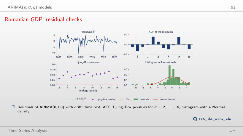
                                                      Slide 61: Romanian GDP: residual checks
                                                      Slide 61
                                                        Question for the room ARIMA(2,1,2) has the smallest Q*(8) of the nine models, 3.28. Is this an argument for it?
                                                        Answer

                                                        No: the optimisation did not converge, and its AICc is 495.4, against 491.9 for ARIMA(0,1,0) with drift. ARIMA(0,1,0) already leaves uncorrelated residuals: Q*(8) = 7.3 (p = 0.51), and Q*(12) has p = 0.54. Extra parameters reduce the residual autocorrelation mechanically. What remains in every model are the fat tails: for ARIMA(0,1,0), kurtosis 7.9, Jarque–Bera 145 and the residual of −11.0 in 2009Q1.

                                                        Interpreting the residual checks
                                                        Slide 62: Interpreting the residual checks
                                                        Slide 62

                                                        Worked example

                                                        \[Q^*(m)=T(T+2)\sum_{h=1}^{m}\frac{\hat\rho_{\hat\varepsilon}(h)^2}{T-h}\approx\chi^2(m-p-q),\qquad \mathrm{JB}=\frac{T}{6}\Big(S^2+\frac{(K-3)^2}{4}\Big)\approx\chi^2(2)\]
                                                          Question for the room For ARIMA(1,1,1), with how many degrees of freedom is Q*(8) compared?
                                                          Answer

                                                          With m − p − q = 8 − 2 = 6: Q*(8) = 5.81 and p = 0.44. For ARIMA(0,1,0), Q*(8) = 7.28 with 8 degrees of freedom and p = 0.51. Without the correction, the p-values of models with ARMA parameters would be too large.

                                                          Forecasting with ARIMA
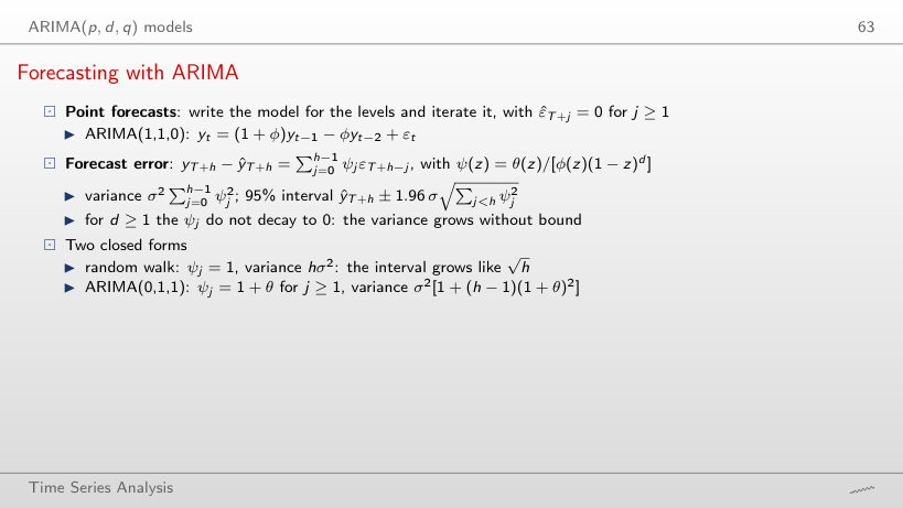
                                                          Slide 63: Forecasting with ARIMA
                                                          Slide 63

                                                          Worked example

                                                          \[\begin{gathered}\text{DS}:\ \Delta y_t=c+\varepsilon_t\ \Rightarrow\ \mathrm{Var}(e_{T+h})=h\sigma^2;\qquad \text{TS}:\ y_t=\alpha+\beta t+u_t,\ u_t=\phi u_{t-1}+\varepsilon_t\\ \Rightarrow\ \mathrm{Var}(e_{T+h})=\sigma^2\frac{1-\phi^{2h}}{1-\phi^2}\ \to\ \frac{\sigma^2}{1-\phi^2},\qquad \text{half-width}=1.96\sqrt{\mathrm{Var}(e_{T+h})}\end{gathered}\]
                                                              Question for the room At h = 40 quarters (10 years), how many times wider is the DS interval than the TS one?
                                                              Answer

                                                              2.53 times: 30.6% against 12.1% of GDP. The TS interval stops at 1.96σ̂/√(1 − φ̂²) = 12.09, while the DS one grows like √h. At h = 12 the half-widths are 16.8% and 11.2%, as on the slide.

                                                              Worked example: ARIMA(1,1,0) forecasts
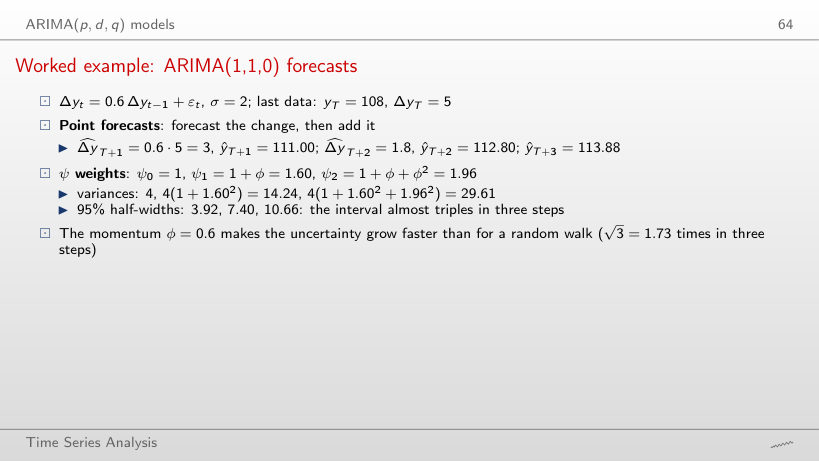
                                                              Slide 64: Worked example: ARIMA(1,1,0) forecasts
                                                              Slide 64

                                                              Worked example

                                                              \[\begin{gathered}\widehat{\Delta y}_{T+h}=\phi\,\widehat{\Delta y}_{T+h-1}=\phi^h\Delta y_T,\qquad \hat y_{T+h}=\hat y_{T+h-1}+\widehat{\Delta y}_{T+h},\\ \psi_j=1+\phi+\dots+\phi^j,\qquad \mathrm{Var}(e_{T+h})=\sigma^2\sum_{j=0}^{h-1}\psi_j^2,\qquad \hat y_{T+h}\pm1.96\sqrt{\mathrm{Var}(e_{T+h})}\end{gathered}\]
                                                                  Question for the room With φ = 0 (a random walk without drift), what do the forecasts and the half-widths become for h = 1, 2, 3?
                                                                  Answer

                                                                  The forecasts are all 108, and the half-widths 3.92, 5.54 and 6.79 = 1.96 · 2 · √h. With φ = 0.6 the forecasts rise to 111.00, 112.80 and 113.88, and the half-widths to 3.92, 7.40 and 10.66: the momentum passes each shock on to the following changes as well.

                                                                  How fast the intervals grow
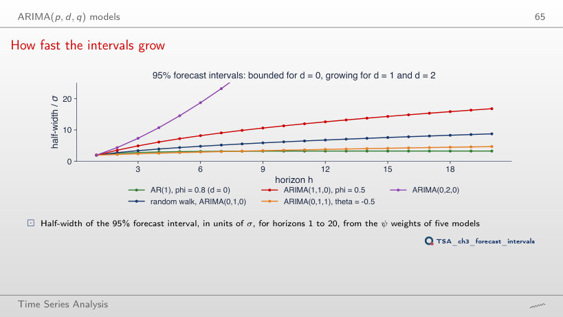
                                                                  Slide 65: How fast the intervals grow
                                                                  Slide 65
                                                                    Question for the room The ▶ button moves θ of the ARIMA(0,1,1) from −0.95 to 0.95. How does the half-width of the interval at h = 20 change?
                                                                    Answer

                                                                    It rises with θ: 2.14σ at θ = −0.9, 4.70σ at θ = −0.5, 8.77σ at θ = 0 (the random walk) and 12.96σ at θ = 0.5. The variance is σ²[1 + (h − 1)(1 + θ)²]: a negative θ offsets part of every shock. For the ARIMA(1,1,0), the half-width at h = 20 is 16.78σ with φ = 0.5 (the chart) and 20.53σ with φ = 0.6 (the worked example, where at h = 3 it is 5.33σ, i.e. 10.66 with σ = 2). The AR(1) with φ = 0.8 levels off at 3.27σ.

                                                                    Interpreting the interval widths
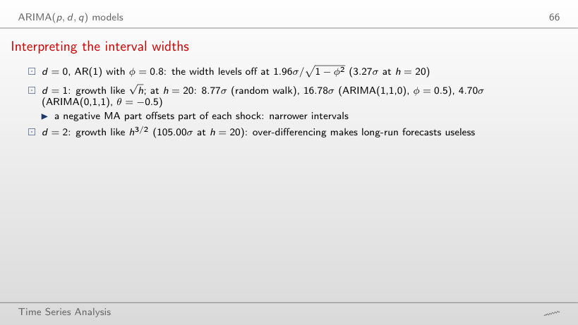
                                                                    Slide 66: Interpreting the interval widths
                                                                    Slide 66

                                                                    Worked example

                                                                    \[\frac{\text{half-width}}{\sigma}=1.96\sqrt{\sum_{j=0}^{h-1}\psi_j^2},\qquad \psi(z)=\frac{\theta(z)}{\phi(z)(1-z)^d}\]
                                                                        Question for the room The interpretation slide gives 16.78σ at h = 20 for ARIMA(1,1,0); the worked example uses φ = 0.6. Which φ produced 16.78σ?
                                                                        Answer

                                                                        φ = 0.5, the value of the chart. With φ = 0.6 the half-width at h = 20 is 20.53σ. At h = 1 both give 1.96σ, and at h = 4: 6.14σ (φ = 0.5) and 6.83σ (φ = 0.6). The random walk has 8.77σ at h = 20.

                                                                        Romanian GDP: two forecasts
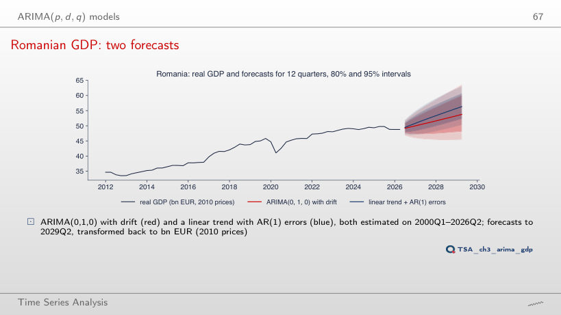
                                                                        Slide 67: Romanian GDP: two forecasts
                                                                        Slide 67
                                                                          Question for the room With the origin in 2019Q4, the two models forecast GDP for 12 quarters. Which one had the smaller error on the observed quarters?
                                                                          Answer

                                                                          The trend-stationary model, but only just: RMSE 7.2 log points, against 7.6 for ARIMA(0,1,0) with drift; both missed the 2020 drop. From 2015Q4 the gap is larger (2.6 against 4.7), and from 2023Q2 the ranking reverses (6.5 against 5.6). From 2026Q2, ARIMA(0,1,0) gives 53.8 bn EUR (2010 prices) after 12 quarters, with a 95% half-width of 16.8 log points; the trend model gives 56.3 bn and 11.2. ADF and KPSS classify the level of GDP as I(1) (p = 0.43; 0.198 > 0.146), but the low power of the tests does not rule out the trend model: the choice of d changes the forecast and its interval.

                                                                          Interpreting the GDP forecasts
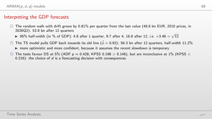
                                                                          Slide 68: Interpreting the GDP forecasts
                                                                          Slide 68
                                                                            Question for the room The slide says that the tests favour DS at 5% but are inconclusive at 1%, while the unit-root table classifies GDP as I(1). How do the two fit?
                                                                            Answer

                                                                            At 5%, ADF does not reject (p = 0.43) and KPSS rejects (0.198 > 0.146): I(1). The evidence is weak, though: at 1% KPSS no longer rejects (0.198 < 0.216), and with T ≈ 100 the power of ADF at φ = 0.9 is 19%. The choice of d matters: after 12 quarters, 53.8 bn EUR with half-width 16.8% (DS) against 56.3 bn EUR with 11.2% (TS).

                                                                            Over-differencing Romanian GDP
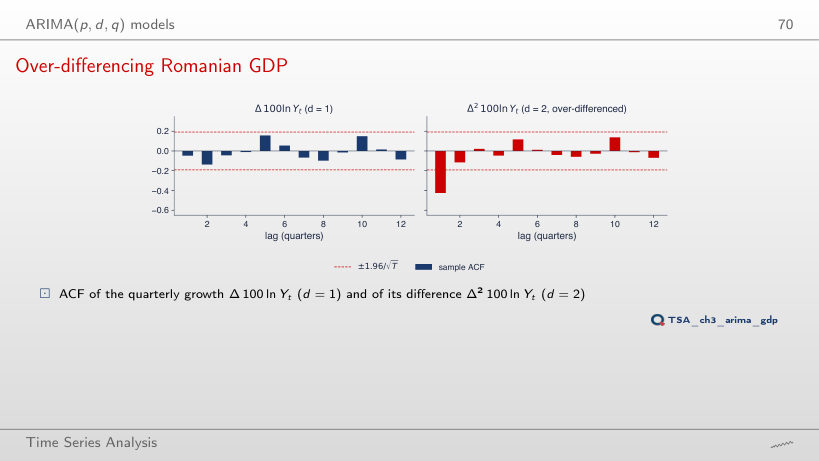
                                                                            Slide 70: Over-differencing Romanian GDP
                                                                            Slide 70
                                                                              Question for the room For US GDP, which symptoms of over-differencing appear with a second difference?
                                                                              Answer

                                                                              All three: ρ̂(1) falls from 0.13 to −0.49, the variance rises from 1.22 to 2.12, and an MA(1) fitted to Δ² gives θ̂ = −0.986 (SE 0.008). For Romania: ρ̂(1) from −0.05 to −0.43, the variance from 6.16 to 12.80, θ̂ = −0.987 (SE 0.080). A third difference makes the symptoms worse: for Romania the variance rises to 35.6 and ρ̂(1) to −0.57.

                                                                              ARIMA in practice

                                                                              Romanian inflation: d = 0 or d = 1?
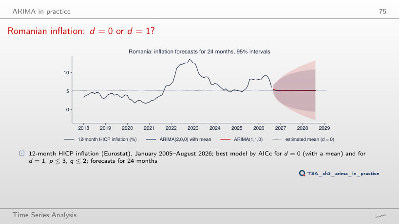
                                                                              Slide 75: Romanian inflation: d = 0 or d = 1?
                                                                              Slide 75
                                                                                Question for the room The lowest AICc for d = 1, 451.2 (ARIMA(1,1,0)), is below the one for d = 0, 455.6 (ARIMA(2,0,0)). Does this show that d = 1 is the better choice?
                                                                                Answer

                                                                                No: AICc does not compare models with different d, because with d = 1 the likelihood is computed for Δπ, another series. We choose d by tests and judgement: KPSS (0.404 < 0.463) keeps d = 0, ADF (p = 0.32) suggests d = 1. The forecasts after 24 months are close, 5.1% and 5.2%, but the 95% intervals differ: [−0.6, 10.9] and [−2.9, 13.3]. ARIMA(3,1,2) has an AICc of 441.1, but its optimisation did not converge.

                                                                                EUR/RON: ARIMA against the random walk
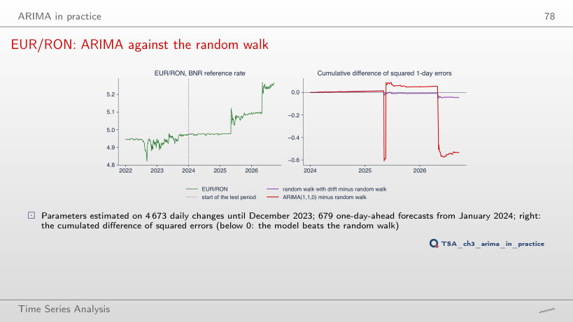
                                                                                Slide 78: EUR/RON: ARIMA against the random walk
                                                                                Slide 78
                                                                                  Question for the room With the test period starting in January 2015, does the ARIMA(1,1,0) still beat the random walk one day ahead?
                                                                                  Answer

                                                                                  No: RMSE 0.1307, against 0.1304 for the random walk, a loss of 0.19%. With the test period from 2019, 2020, 2022 or 2024, the gain is 2.1–2.3%; in the lecture (from 2024), 0.1300 against 0.1330, and over 20 days 0.638 against 0.667 (4.3%). The gain depends on the period chosen and comes from a few days with jumps of the rate; a formal comparison needs the Diebold–Mariano test.

                                                                                  A classic series: US real GDP after 2007
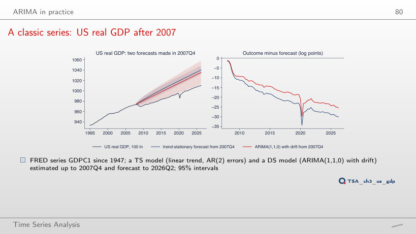
                                                                                  Slide 80: A classic series: US real GDP after 2007
                                                                                  Slide 80
                                                                                    Question for the room With the origin in 2007Q4, the trend-stationary model misses by −30 log points at the end. Is the error specific to 2007? Move the origin to 2000Q4.
                                                                                    Answer

                                                                                    No: from 2000Q4, the gap at the end is −34.7 for the trend model (half-width of the 95% interval: 7.9) and −34.5 for ARIMA(1,1,0) with drift (28.1). From 2007Q4: −30.1 (8.2) and −25.4 (22.9); from 2019Q4: −8.0 (11.1) and −5.0 (13.2). From 2000 and from 2007 neither interval covers the outcome; from 2019 both do. Both models extend the drift from before the origin, and growth after 2008 was slower.

                                                                                    Simulations: shocks from the Normal distribution, drawn with the seeds of the chapter code; the Monte Carlo results are those of the lecture. Romanian GDP: Eurostat, chain-linked volumes (2010 prices), seasonally adjusted, in the version used in the lecture. HICP: Eurostat, up to August 2026. EUR/RON: BNR reference rate; BET and S&P 500: the course market data, up to 18 September 2026. US GDP: FRED GDPC1, up to 2026Q2. Nile: the statsmodels data set, 1871–1970.