

Time Series Analysis

Chapter 6 · VAR Models and Granger Causality

The slide of the lecture is on the left, the same figure or table on the right, computed in the browser from the same data. The ▶ button moves the parameter step by step; the “Worked example” boxes redo the calculation with the numbers of the chapter.

From one series to several · The VAR(p) model · Stationarity and the companion form · Estimation and lag selection · Residual diagnostics · Granger causality · Impulse responses · Forecast error variance decomposition · Forecasting with a VAR · Structural VARs and a landmark case study

From one series to several

Romania: four macro series that move together
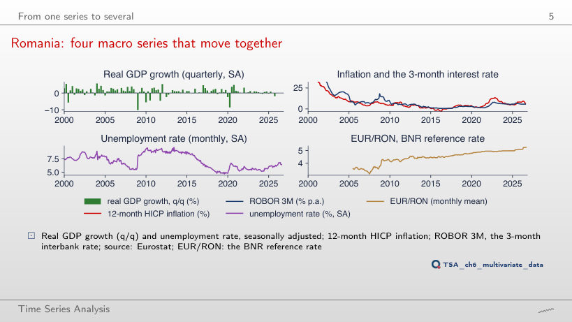
Slide 5: Romania: four macro series that move together
Slide 5
    Question for the room Move the start of the window to 2015. What does the correlation between inflation and ROBOR 3M become?
    Answer

    0.89, against 0.66 over 2005–2026. After 2015 the two series rose and fell together (inflation reached 13.6% in November 2022, ROBOR 3M 8.0% in October 2022), and the 2008 episode, when ROBOR reached 18.2% in the liquidity crisis, has left the window. The correlation between the levels of two persistent series depends strongly on the sample and does not say which of them leads the other.

    Cross-correlations: markets and Romanian macro data
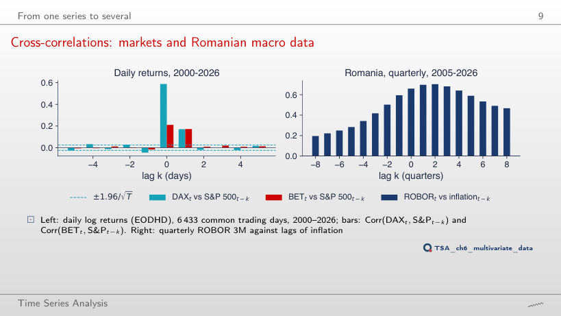
    Slide 9: Cross-correlations: markets and Romanian macro data
    Slide 9
      Question for the room Start the daily returns in 2015. Is the correlation between yesterday’s DAX and today’s S&P 500 (k = −1) inside the band?
      Answer

      No: −0.058, outside the band ±0.037; over the whole sample it is −0.046, also outside the band ±0.024. The lead runs mainly from New York to Europe (0.135 at k = 1 since 2015, 0.171 over the whole sample), but not in one direction only: yesterday’s DAX also has a small negative correlation with today’s S&P 500. For the BET the value at k = −1 (−0.005 since 2015, −0.017 over the whole sample) stays inside the band.

      The VAR(p) model

      Worked example: a VAR(1)
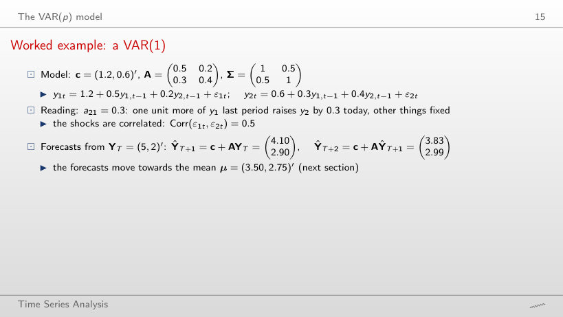
      Slide 15: Worked example: a VAR(1)
      Slide 15

      Worked example

      \[\hat{\mathbf Y}_{T+h}=\mathbf c+\mathbf A\hat{\mathbf Y}_{T+h-1},\quad \boldsymbol\mu=(\mathbf I-\mathbf A)^{-1}\mathbf c,\quad \lambda^2-\mathrm{tr}(\mathbf A)\lambda+\det(\mathbf A)=0,\quad \boldsymbol\Sigma(h)=\sum_{s=0}^{h-1}\mathbf A^{s}\boldsymbol\Sigma\mathbf A^{s\prime}\]
          Question for the room Set a₁₂ = 0.5 and a₂₁ = 0.8. All coefficients of A are below 1. Is the VAR stable?
          Answer

          No. tr(A) = 0.9 and det(A) = 0.5·0.4 − 0.5·0.8 = −0.20, so λ = (0.9 ± √1.61)/2: λ₁ = 1.084 and λ₂ = −0.184. The largest modulus exceeds 1 and the forecasts grow without bound (ŷ₁ = 16.48 at h = 8). Stability depends on the eigenvalues, not on the size of each coefficient: the cross effects a₁₂a₂₁ = 0.40 add to the own persistence. With a₁₁ = 0.5 and a₂₂ = 0.4, the VAR is stable only if a₁₂a₂₁ < 0.30.

          The worked example, simulated
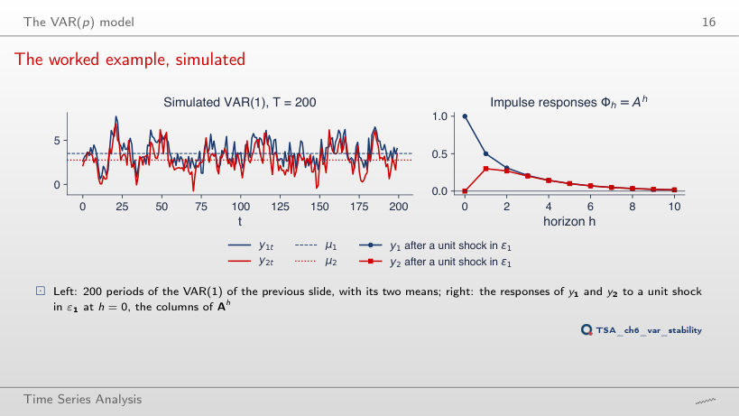
          Slide 16: The worked example, simulated
          Slide 16

          Worked example

          \[\boldsymbol\Phi_h=\mathbf A\boldsymbol\Phi_{h-1}=\mathbf A^h,\qquad \boldsymbol\Phi_h\mathbf e_1=w_1\lambda_1^h\mathbf v_1+w_2\lambda_2^h\mathbf v_2\]
              Question for the room Move a₂₁ to 0.6 (λ₁ = 0.8). What is the response of y₁ after 5 periods, Φ₁₁(5)?
              Answer

              0.187, not 0.8⁵ = 0.328. Φ₁₁(h) = 0.571·0.8ʰ + 0.429·0.1ʰ: the dominant component enters e₁ with weight 0.571, and the ratio Φ₁₁(h)/Φ₁₁(h−1) approaches 0.8 only after a few periods. The same holds in the lecture’s example: Φ₁₁(5) = 0.6·0.7⁵ + 0.4·0.2⁵ = 0.101, so after 5 periods about 0.10 of the initial effect is left; 0.7⁵ ≈ 0.17 is the factor by which the dominant component shrinks, not the response.

              Stationarity and the companion form

              Eigenvalues of three estimated VARs
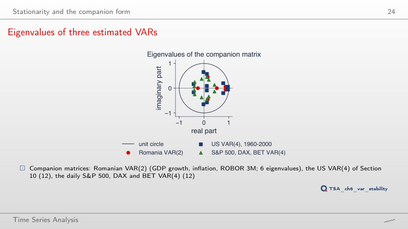
              Slide 24: Eigenvalues of three estimated VARs
              Slide 24
                Question for the room With p = 5, the order chosen by AIC, what is the largest modulus and how many eigenvalues does the companion matrix have?
                Answer

                0.913, out of 15 eigenvalues (the companion matrix is 15 × 15), against 0.869 out of 6 for p = 2; a shock halves after 7.7 quarters, against 5.0. Extra lags add eigenvalues, and some with a large modulus (0.874, 0.836) come in complex pairs, i.e. oscillations that the VAR(2) does not have. With 48 coefficients on about 80 quarters, these oscillations may be estimation noise.

                Estimation and lag selection

                Romanian VAR: which p?
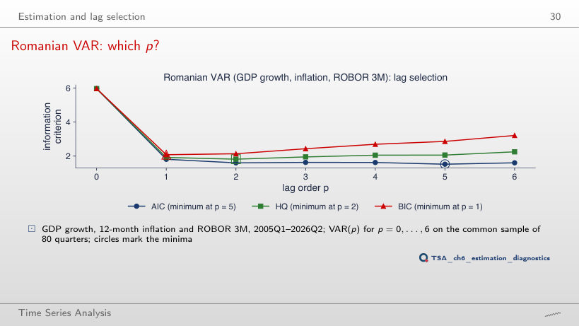
                Slide 30: Romanian VAR: which p?
                Slide 30

                Worked example

                \[\mathrm{IC}(p)=\ln\det\tilde{\boldsymbol\Sigma}(p)+c_T\,\frac{pK^2}{T},\qquad c_T=2\ (\mathrm{AIC}),\ \ 2\ln\ln T\ (\mathrm{HQ}),\ \ \ln T\ (\mathrm{BIC})\]
                    Question for the room End the sample in 2019 (pmax = 6). Which order does HQ choose?
                    Answer

                    p = 5, like AIC; BIC still chooses p = 1. The common sample has only T = 54 quarters, and ln det Σ̃(5) = −0.446 is far below the value for p = 2 (0.970), because a VAR(5) has 48 coefficients for 54 observations and almost reproduces the data. The HQ penalty, 2 ln ln T = 2.767 per unit of pK²/T, does not offset it. In short samples the criteria can choose large orders: check how many degrees of freedom are left.

                    The estimated Romanian VAR(2)
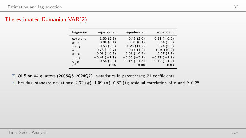
                    Slide 32: The estimated Romanian VAR(2)
                    Slide 32
                      Question for the room End the sample in 2019Q4. Does the coefficient of gt−1 in the ROBOR equation stay significant (|t| ≥ 2)?
                      Answer

                      Yes: 0.21 with t = 3.7, against 0.14 with t = 3.5 over the whole sample; in addition gt−2 becomes significant (0.14, t = 2.3). Without 2020–2026 the R² of the GDP equation rises from 0.16 to 0.30, because the pandemic quarter, with its residual of −9.1, is no longer in the sample. The link between GDP growth and next quarter’s interest rate does not come from the pandemic years.

                      Residual diagnostics

                      Residuals of the Romanian VAR(2)
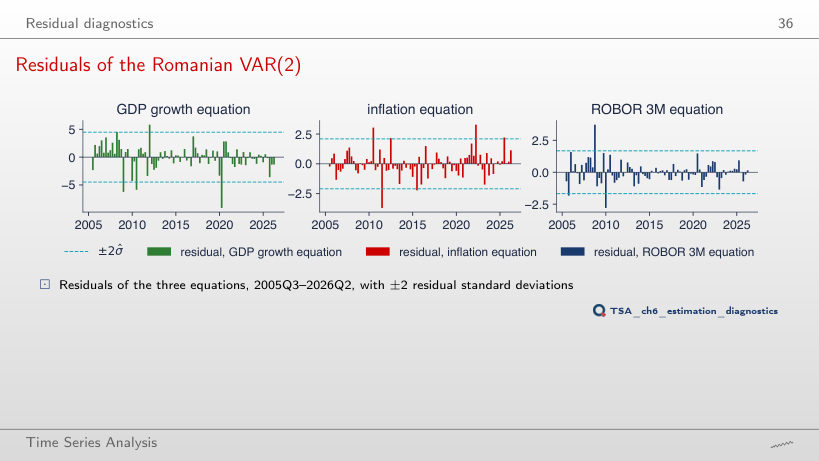
                      Slide 36: Residuals of the Romanian VAR(2)
                      Slide 36

                      Worked example

                      \[Q_h=T^2\sum_{j=1}^{h}\frac{1}{T-j}\,\mathrm{tr}\big(\hat{\mathbf C}_j^{\prime}\hat{\mathbf C}_0^{-1}\hat{\mathbf C}_j\hat{\mathbf C}_0^{-1}\big)\sim\chi^2\big(K^2(h-p)\big)\]
                          Question for the room Add dummies for 2009Q1 and 2020Q2. Does the Jarque–Bera test still reject normality of the residuals?
                          Answer

                          Yes: the statistic falls from 191 to 144 (χ²(6), p < 0.001). The dummies cancel the residuals of the two quarters, but other extreme values remain: ROBOR +3.5 in 2008Q4, inflation −3.7 in 2011Q3, GDP −5.9 in 2010Q3; the kurtosis of ROBOR stays 7.9. The portmanteau test even gets worse (Q₈ = 88.2, p = 0.002): removing two observations does not make the residuals Normal white noise.

                          Granger causality

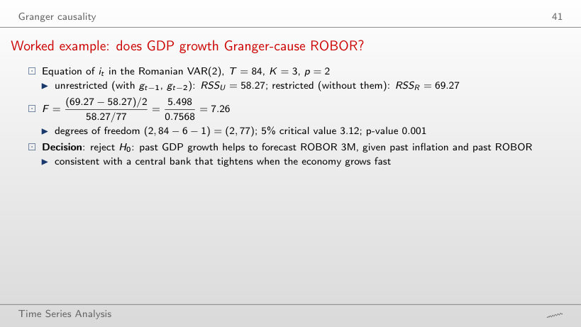
                          Worked example: does GDP growth Granger-cause ROBOR?
                          Slide 41: Worked example: does GDP growth Granger-cause ROBOR?
                          Slide 41

                          Worked example

                          \[F=\frac{(RSS_R-RSS_U)/p}{RSS_U/(T-Kp-1)}\sim F(p,\,T-Kp-1),\qquad W=pF\sim\chi^2(p)\]
                              Question for the room Move to p = 4. What are F and its degrees of freedom for GDP growth → ROBOR 3M?
                              Answer

                              F = 8.50 with (4, 69) degrees of freedom, p < 0.001; the 5% critical value falls to 2.50. Four restrictions are now tested: RSSR − RSSU = 64.08 − 42.93 = 21.15 is divided by 4, and RSSU by T − Kp − 1 = 82 − 12 − 1 = 69. The conclusion does not depend on p: with p = 1, F = 10.63 (p = 0.002).

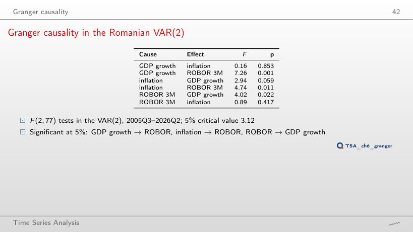
                              Granger causality in the Romanian VAR(2)
                              Slide 42: Granger causality in the Romanian VAR(2)
                              Slide 42
                                Question for the room End the sample in 2019Q4 (three-variable VAR). Does inflation → ROBOR 3M stay significant at 5%?
                                Answer

                                No: F = 2.46, p = 0.096, against 4.74 (p = 0.011) over the whole sample. On the other hand, inflation → GDP growth becomes significant (F = 6.27, p = 0.004). Without 2021–2023, when inflation climbed to 13.6% and ROBOR rose with it, the link from inflation to ROBOR is no longer separated from noise on 58 quarters. Granger results depend on the sample, not only on the set of variables.

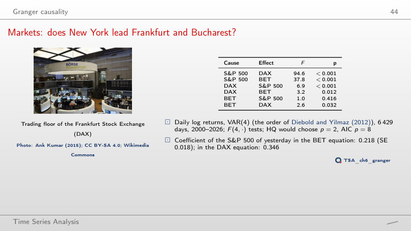
                                Markets: does New York lead Frankfurt and Bucharest?
                                Slide 44: Markets: does New York lead Frankfurt and Bucharest?
                                Slide 44
                                  Question for the room Start the sample in 2010. Does DAX → BET stay significant at 5%?
                                  Answer

                                  No: F = 1.1, p = 0.369 (over 2000–2026: F = 3.2, p = 0.012). S&P 500 → BET stays very strong (F = 22.5), and the coefficient of yesterday’s S&P 500 in the BET equation falls from 0.218 to 0.183. With 4,033 days the test has a lot of power, so p = 0.369 shows that the DAX → BET effect, given the S&P 500, is small after 2010; it does not show that it is exactly zero.

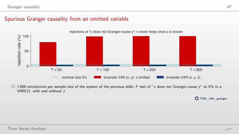
                                  Spurious Granger causality from an omitted variable
                                  Slide 47: Spurious Granger causality from an omitted variable
                                  Slide 47
                                    Question for the room Set the effect of z on y to 0. What rejection rate does the VAR without z have at T = 500?
                                    Answer

                                    5.6%, close to the nominal 5% (between 4.5% and 5.6% for all sample sizes), against 100% with the effect 0.8 and 100% with 0.4. x looks like a cause of y only because xt−1 is a noisy measure of zt−2, which drives yt. The lag order matters too: with p = 1 even the VAR with z rejects in 76%–100% of the cases, because one lag of z does not contain zt−2, and xt−1 stands in for it.

                                    Impulse responses

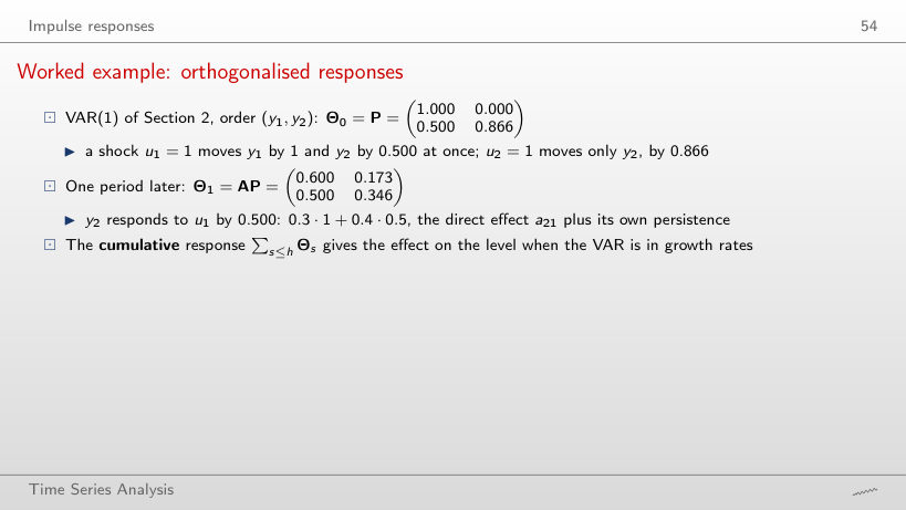
                                    Worked example: orthogonalised responses
                                    Slide 54: Worked example: orthogonalised responses
                                    Slide 54

                                    Worked example

                                    \[\boldsymbol\Sigma=\mathbf P\mathbf P^{\prime},\qquad \boldsymbol\Theta_0=\mathbf P,\qquad \boldsymbol\Theta_h=\boldsymbol\Phi_h\mathbf P=\mathbf A\boldsymbol\Theta_{h-1}\]
                                        Question for the room Put y₂ first in the Cholesky ordering. What is the response of y₂ to the shock u₁ on impact and one period later?
                                        Answer

                                        0 on impact and 0.260 one period later (0.3·0.866 + 0.4·0), against 0.500 and 0.500 in the order (y₁, y₂). With y₂ first, the whole correlation of 0.5 is assigned to the shock u₂, which moves y₁ by 0.500 on impact; u₁ reaches y₂ only through a₂₁, one period later. The same VAR and the same data give different responses: the ordering is an assumption.

                                        Impulse responses of the Romanian VAR(2)
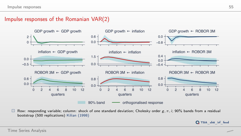
                                        Slide 55: Impulse responses of the Romanian VAR(2)
                                        Slide 55

                                        Worked example

                                        \[\theta_{jk,h}=\sum_{m=1}^{K}\phi_{jm,h}\,p_{mk},\qquad \boldsymbol\Theta_h=\boldsymbol\Phi_h\mathbf P,\quad \boldsymbol\Sigma=\mathbf P\mathbf P^{\prime}\]
                                            Question for the room Put ROBOR first (order i, g, π). What is the response of ROBOR to the inflation shock on impact and after 4 quarters?
                                            Answer

                                            0 on impact, by construction, and 0.64 pp after 4 quarters, against 0.23 and 0.82 pp in the lecture’s ordering; the band excludes zero at 9 of the 13 horizons, against 11. With ROBOR first, the common part of the two shocks (residual correlation 0.25) is assigned to ROBOR. The qualitative conclusion stays: ROBOR rises after an inflation shock and stays higher for years (0.38 pp after 12 quarters).

                                            Does the ordering change the answer?
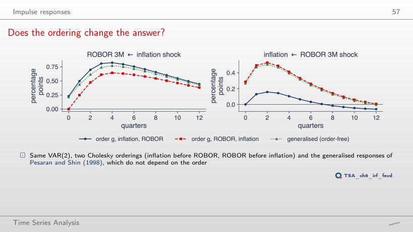
                                            Slide 57: Does the ordering change the answer?
                                            Slide 57

                                            Worked example

                                            \[\boldsymbol\Theta_0=\mathbf P\ \ (\text{Cholesky}),\qquad \boldsymbol\psi_k(0)=\boldsymbol\Sigma\mathbf e_k/\sqrt{\sigma_{kk}}\ \ (\text{generalised})\]
                                                Question for the room Move to p = 1. Does inflation still rise after a ROBOR shock (the “price puzzle”) when inflation comes before ROBOR?
                                                Answer

                                                No: the largest response is 0.00 pp, on impact (zero by the ordering), and the response is negative afterwards; with p = 2 it rose to 0.16 pp. With ROBOR first, the impact is 0.29 pp in the VAR(1) as well, because the ordering assigns the common part of the shocks to ROBOR. The “puzzle” depends here on both the ordering and the number of lags: a result that changes with p and with the ordering is fragile.

                                                Markets: responses to an S&P 500 shock
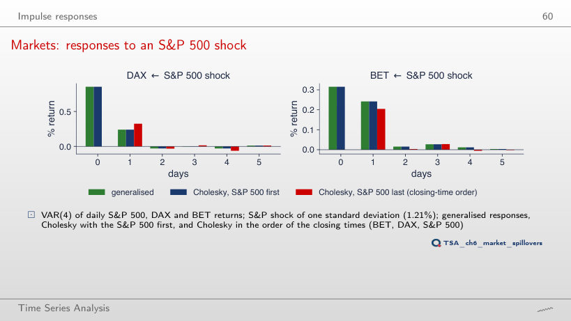
                                                Slide 60: Markets: responses to an S&P 500 shock
                                                Slide 60

                                                Worked example

                                                \[\boldsymbol\psi_{S}(0)=\frac{\boldsymbol\Sigma\mathbf e_{S}}{\sqrt{\sigma_{SS}}},\qquad \psi_{j}(0)=\frac{\sigma_{jS}}{\sqrt{\sigma_{SS}}}=\rho_{jS}\,\sqrt{\sigma_{jj}},\quad S=\text{S\&P 500}\]
                                                    Question for the room Start the sample in 2015. What does the generalised response of the BET the day after an S&P 500 shock become?
                                                    Answer

                                                    0.11%, against 0.24% over 2000–2026; the same-day response stays 0.32%. For the DAX the response falls from 0.85% to 0.68% on the same day and from 0.24% to 0.16% the next day. The next-day part, which comes from the different closing times, is about half as large after 2015.

                                                    Forecast error variance decomposition

                                                    Forecast error variance decomposition
                                                    Slide 63: Forecast error variance decomposition
                                                    Slide 63

                                                    Worked example

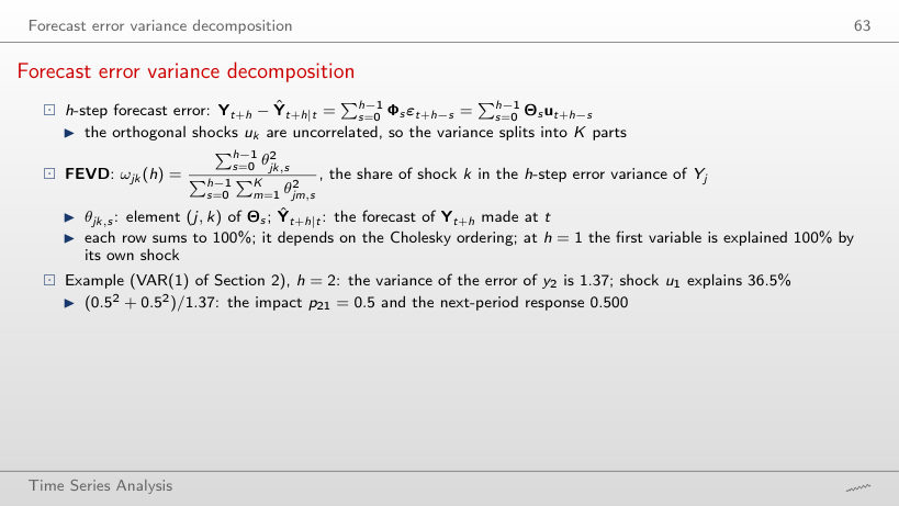
                                                    \[\omega_{jk}(h)=\frac{\sum_{s=0}^{h-1}\theta_{jk,s}^2}{\sum_{s=0}^{h-1}\sum_{m=1}^{K}\theta_{jm,s}^2}\]
                                                        Question for the room Put y₂ first. What share of the 10-step forecast error variance of y₂ is due to u₁?
                                                        Answer

                                                        10.6%, against 45.8% in the order (y₁, y₂); at one step the share is 0%. With y₂ first, u₁ reaches y₂ only through a₂₁ = 0.3, one period later (0.260 at h = 1), and the sum of the squares of these responses is 0.182 out of 1.724. The error variance does not change (1.72 at h = 10 in both orders); only its split between the shocks does.

                                                        FEVD of the Romanian VAR(2)
                                                        Slide 64: FEVD of the Romanian VAR(2)
                                                        Slide 64

                                                        Worked example

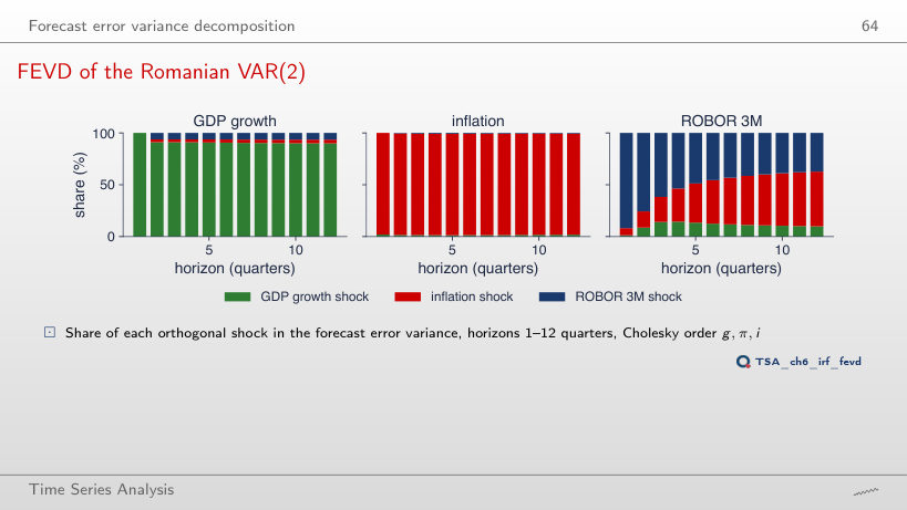
                                                        \[\omega_{i\pi}(h)=\frac{\sum_{s=0}^{h-1}\theta_{i\pi,s}^2}{\sum_{s=0}^{h-1}\big(\theta_{ig,s}^2+\theta_{i\pi,s}^2+\theta_{ii,s}^2\big)}\]
                                                            Question for the room Choose the order i, π, g (ROBOR first). How much of the 12-quarter forecast error variance of ROBOR do inflation shocks explain?
                                                            Answer

                                                            27%, against 53% in the lecture’s ordering; ROBOR’s own shocks explain 63% instead of 37%. At one quarter ROBOR is explained 100% by its own shock, by construction. The conclusion that in the long run the interest rate is driven mainly by inflation therefore rests on the assumption that ROBOR reacts to inflation within the quarter, not the other way round.

                                                            Spillover table: S&P 500, DAX, BET
                                                            Slide 67: Spillover table: S&P 500, DAX, BET
                                                            Slide 67

                                                            Worked example

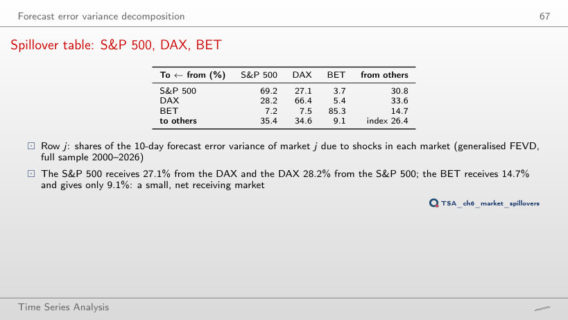
                                                            \[S(H)=\frac{100}{K}\sum_{j\ne k}\tilde\omega_{jk}(H),\qquad \text{to}_k=100\sum_{j\ne k}\tilde\omega_{jk},\quad \text{from}_j=100\sum_{k\ne j}\tilde\omega_{jk},\quad \text{net}_k=\text{to}_k-\text{from}_k\]
                                                                Question for the room Choose the year 2020. What share of the forecast error variance of the BET comes from the other markets?
                                                                Answer

                                                                49.0%, against 14.7% over 2000–2026; the index rises to 51.2% (26.4% over the whole sample), and the BET transmits 45.3% instead of 9.1%. In the pandemic year the markets moved together. A single year has only 237 days for the 39 coefficients of the VAR(4), so the table of one year is noisier; in 2017, a calm year, the index is 24.4% and the BET receives 13.2%.

                                                                The spillover index over time
                                                                Slide 68: The spillover index over time
                                                                Slide 68
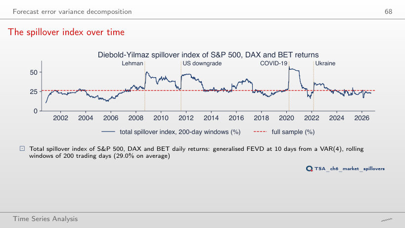
                                                                  Question for the room Widen the window to 500 days. What does the maximum of the index become, and when does it occur?
                                                                  Answer

                                                                  47.3%, on 22 September 2021, against 57.5% on 17 March 2020 with 200-day windows. A longer window mixes the crash of March 2020 with more calm days, so the peak is lower and comes later; the mean stays almost the same (29.1% against 29.0%). The size and date of the peaks depend on the window length: part of the jumps is mechanical.

                                                                  Forecasting with a VAR

                                                                  Romanian VAR(2): forecasts for two years
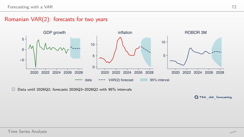
                                                                  Slide 72: Romanian VAR(2): forecasts for two years
                                                                  Slide 72

                                                                  Worked example

                                                                  \[\hat{\mathbf Y}_{T+1|T}=\mathbf c+\mathbf A_1\mathbf Y_T+\mathbf A_2\mathbf Y_{T-1},\qquad \hat Y_{j,T+h|T}\pm1.96\sqrt{\sigma_{jj}(h)},\quad \boldsymbol\Sigma(h)=\sum_{s=0}^{h-1}\boldsymbol\Phi_s\boldsymbol\Sigma\boldsymbol\Phi_s^{\prime}\]
                                                                      Question for the room Move the origin to 2020Q4. Is the inflation realised in 2022Q4 inside the 95% interval of the 8-quarter forecast?
                                                                      Answer

                                                                      No: 13.2% realised, against a forecast of 2.4% and the interval [−2.3; 7.1]. The VAR estimated up to 2020 contains none of the energy-price shocks of 2021–2022, and the interval assumes Normal shocks with the past variance and ignores parameter uncertainty. With the origin 2019Q4, the inflation of 2021Q4 (6.4%) was still inside the interval ([−2.0; 7.7]).

                                                                      VAR against univariate benchmarks
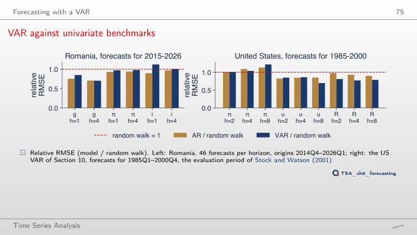
                                                                      Slide 75: VAR against univariate benchmarks
                                                                      Slide 75
                                                                        Question for the room Start the evaluation for Romania in 2021 (h = 1). Is the VAR still significantly less accurate than the AR for GDP growth?
                                                                        Answer

                                                                        Not at 5%: relative RMSE 1.06 for the VAR and 0.76 for the AR, but DM = 1.74, p = 0.082, on only 22 forecasts. The difference still favours the AR, and the VAR is now less accurate than even the random walk; with half the forecasts, the test no longer separates it from noise at 5%.

                                                                        Structural VARs and a landmark case study

                                                                        The three US series
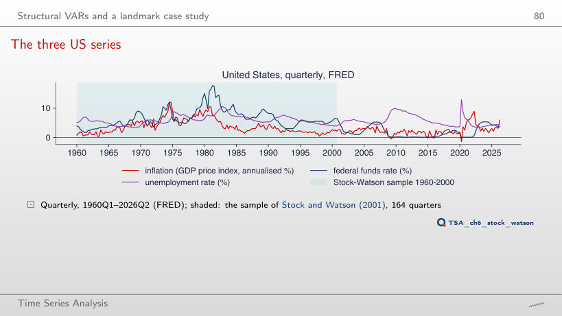
                                                                        Slide 80: The three US series
                                                                        Slide 80
                                                                          Question for the room Extend the window to 2026. What does the mean federal funds rate become?
                                                                          Answer

                                                                          4.78%, against 6.59% in 1960–2000; the correlation of unemployment and the rate falls from 0.29 to 0.05. After 2008 and in 2020 the rate stayed close to zero (minimum 0.06%), and inflation went down to −1.43%. The extended sample contains a regime that the 1960–2000 VAR never saw.

                                                                          Stock–Watson VAR: impulse responses
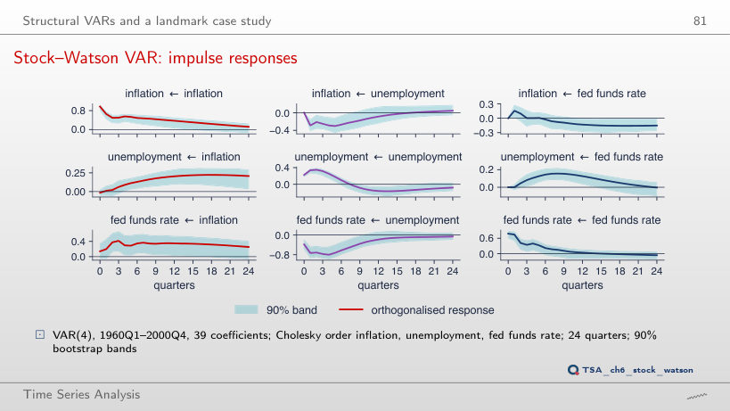
                                                                          Slide 81: Stock–Watson VAR: impulse responses
                                                                          Slide 81
                                                                            Question for the room Extend the sample to 2026Q2. What sign does the response of unemployment to a monetary shock have after 2 quarters?
                                                                            Answer

                                                                            Negative: −0.13 pp, against +0.05 pp in 1960–2000 (where the peak is 0.16 pp after 8 quarters). The monetary shock now explains only 4% of the 12-quarter variance of unemployment, against 19%. The near-zero rates after 2008 and the pandemic change the system, and a VAR with constant parameters on 1960–2026 mixes different regimes: the wrong sign signals that the model is unstable.

                                                                            Quarterly data for Romania, 2005Q1 – 2026Q2: real GDP growth (Eurostat, the series of the lecture), 12-month HICP inflation and ROBOR 3M (quarterly means). Daily log returns in %, 6,433 common days, 6 January 2000 – 18 September 2026: S&P 500, DAX and BET (EODHD). United States: FRED (GDPCTPI, UNRATE, FEDFUNDS), 1960Q1 – 2026Q2. The VARs, tests, impulse responses, FEVDs and the spillover index are re-estimated in the browser by OLS; the initial states are those of the lecture. The bootstrap bands of the Romanian responses use the draws of the chapter’s seed (500 replications); the simulated VAR(1) uses the Normal draws of the same seed. Variants that do not appear in the lecture (another lag order p, another Cholesky ordering, another sample, other windows, other effects in the simulation) are extra runs of the chapter code with the same data and seed; the spillover index with other windows or another horizon is computed every 5 days.