

Time Series Analysis

Chapter 9 · Machine Learning for Time Series

The slide of the lecture is on the left, the same figure or table on the right, computed in the browser from the same data. The ▶ button moves the parameter step by step; the “Worked example” boxes redo the calculation with the numbers of the chapter.

Forecasting as supervised learning · Validation without leakage · Regularised linear models: ridge and lasso · Trees, random forest and gradient boosting · Neural networks · Application: electricity load against Chapter 4 · Prediction intervals · Local and global models: Romanian inflation · Applications in finance: volatility and the sign of returns · Landmark case studies: M4, M5 and Gu, Kelly and Xiu

Forecasting as supervised learning

Worked example: a lag table for the electricity load
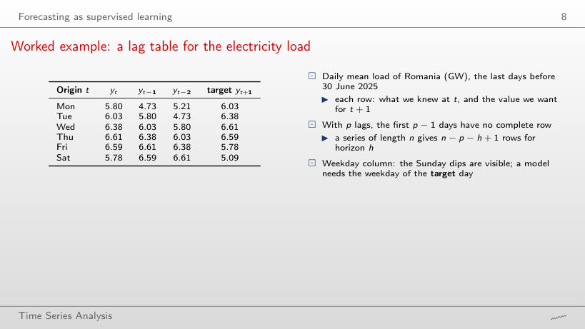
Slide 8: Worked example: a lag table for the electricity load
Slide 8

Worked example

      Question for the room With p = 5 lags and h = 3, how many complete rows do the 9 days give?
      Answer

      9 − 5 − 3 + 1 = 2 rows, with origins 25 and 26 June 2025. On the whole series the table for h = 3 has 1642 − 28 − 3 + 1 = 1612 rows.

      Electricity load: the series and three features
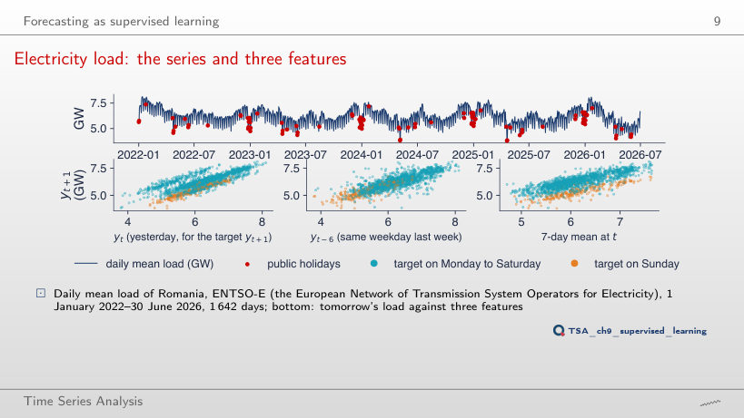
      Slide 9: Electricity load: the series and three features
      Slide 9
        Question for the room Move the horizon to h = 7. What do the correlations of the target with yt and with the 7-day mean become?
        Answer

        0.81 with yt (0.77 at h = 1) and 0.60 with the 7-day mean (0.74 at h = 1). At h = 7 today is the same weekday as the target, so yt takes the role of the weekly lag, while the 7-day mean carries no weekday.

        Recursive, direct and multi-output forecasts
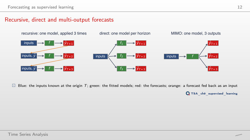
        Slide 12: Recursive, direct and multi-output forecasts
        Slide 12
          Question for the room Choose the origin 6 April 2026, with Easter in the window. Which strategy has the lower MAE over the 14 days?
          Answer

          The direct one: 668 MW against 898 MW for the recursive one. At h = 7 the direct coefficient on yT is 0.81, the implied b⁷ only 0.15: iterating an AR(1) loses the weekly pattern, which the direct model keeps.

          Worked example: recursive and direct two-step forecasts
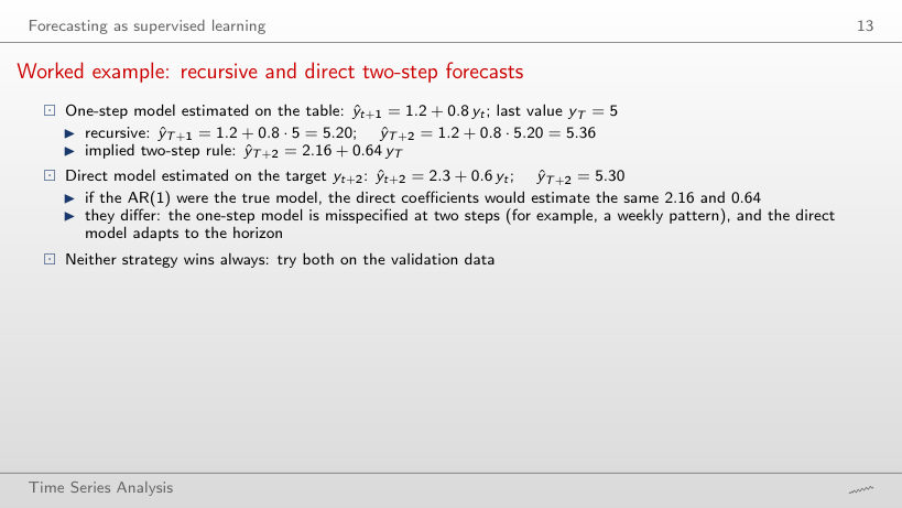
          Slide 13: Worked example: recursive and direct two-step forecasts
          Slide 13

          Worked example

          \[\hat y_{T+1}=a+b\,y_T,\quad \hat y_{T+2}=a+b\,\hat y_{T+1}=a(1+b)+b^2y_T;\qquad \text{direct: }\hat y_{T+2}=2.3+0.6\,y_T\]
              Question for the room Set yT = 7. Which two-step forecast is larger?
              Answer

              The recursive one: 2.16 + 0.64·7 = 6.64, against 2.3 + 0.6·7 = 6.50 for the direct one. The two rules cross at yT = 3.5; above it the recursive rule, with the steeper slope, always gives more.

              Validation without leakage

              Four validation schemes
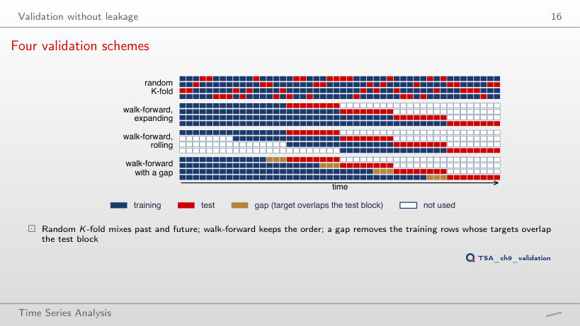
              Slide 16: Four validation schemes
              Slide 16
                Question for the room Move the gap to h = 6. What share of the test rows of walk-forward without a gap has a training row less than 6 steps away?
                Answer

                63% (25% at h = 3); 100% in random K-fold, 0% with a gap. The first h − 1 = 5 of the 8 rows of each test block have targets that overlap the last training rows.

                Leakage in practice: random folds on overlapping targets
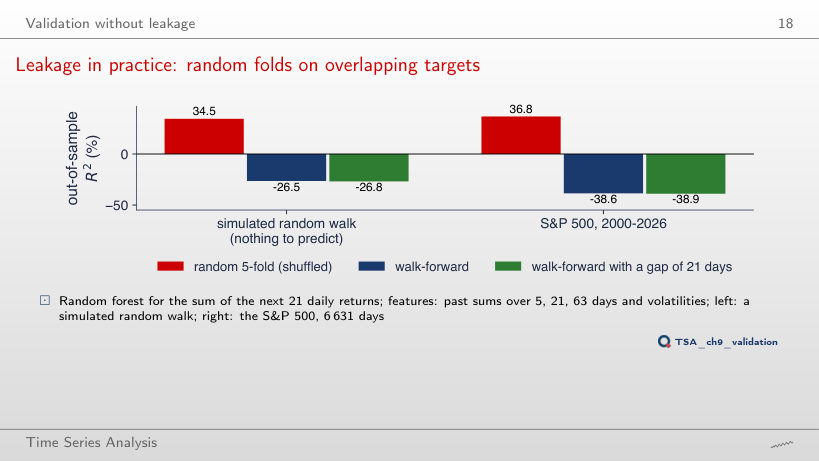
                Slide 18: Leakage in practice: random folds on overlapping targets
                Slide 18
                  Question for the room Choose h = 1: the target is one return, without overlap. What R² does random 5-fold report for the simulated random walk?
                  Answer

                  −4.5%, close to walk-forward (−6.3%) and to walk-forward with a gap (−6.1%). Without overlapping targets a test row has no near-copies in the training folds, and the 34.5% disappears.

                  Interpreting the leakage experiment
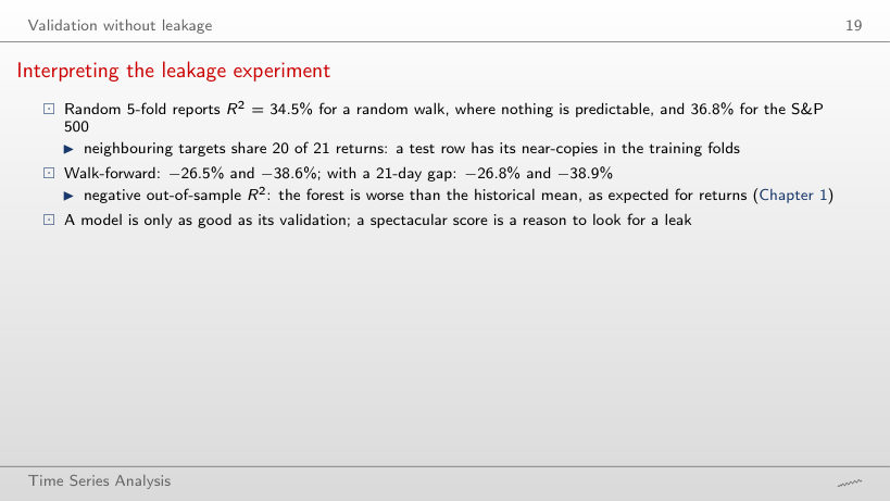
                  Slide 19: Interpreting the leakage experiment
                  Slide 19

                  Worked example

                  \[\rho(Y_t,Y_{t+k})=\max\!\Big(0,1-\frac{k}{h}\Big),\qquad R^2=1-\frac{\sum_{\text{folds}}\sum_t(y_t-\hat y_t)^2}{\sum_{\text{folds}}\sum_t(y_t-\bar y_{\text{train}})^2}\]
                      Question for the room Choose h = 63. What R² do random 5-fold and walk-forward with a gap give for the S&P 500?
                      Answer

                      43.4% and −43.6%. Neighbouring targets share 62 of 63 returns (sample correlation 0.976), so random folds leak even more. Without a gap walk-forward gives −36.2%: the last training rows have targets that overlap the first test rows, a small leak that the gap removes.

                      Bias and variance of regression trees
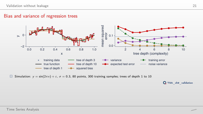
                      Slide 21: Bias and variance of regression trees
                      Slide 21
                        Question for the room Raise the noise to σ = 0.6. At what depth is the expected test error smallest?
                        Answer

                        At depth 2 (0.465; the noise variance is 0.36). With σ = 0.1 the minimum moves to depth 6. More noise raises the variance of deep trees, so the right complexity falls.

                        Regularised linear models: ridge and lasso

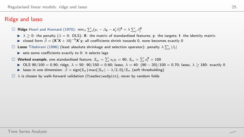
                        Ridge and lasso
                        Slide 25: Ridge and lasso
                        Slide 25

                        Worked example: ridge

                        \[\hat\beta_{\text{ridge}}=\frac{S_{xy}}{S_{xx}+\lambda}=\frac{S_{xx}}{S_{xx}+\lambda}\,\hat\beta_{\text{OLS}}\]

                          Worked example: lasso

                          \[\hat\beta_{\text{lasso}}=\operatorname{sign}(S_{xy})\,\frac{\max(|S_{xy}|-\lambda/2,\,0)}{S_{xx}}\]
                              Question for the room Set Sxy = 30. From what λ is the lasso coefficient exactly 0, and what does ridge give with λ = 50?
                              Answer

                              From λ = 2·30 = 60; ridge gives 30/150 = 0.200, not zero. The lasso threshold grows with |Sxy|: features weakly related to the target leave first.

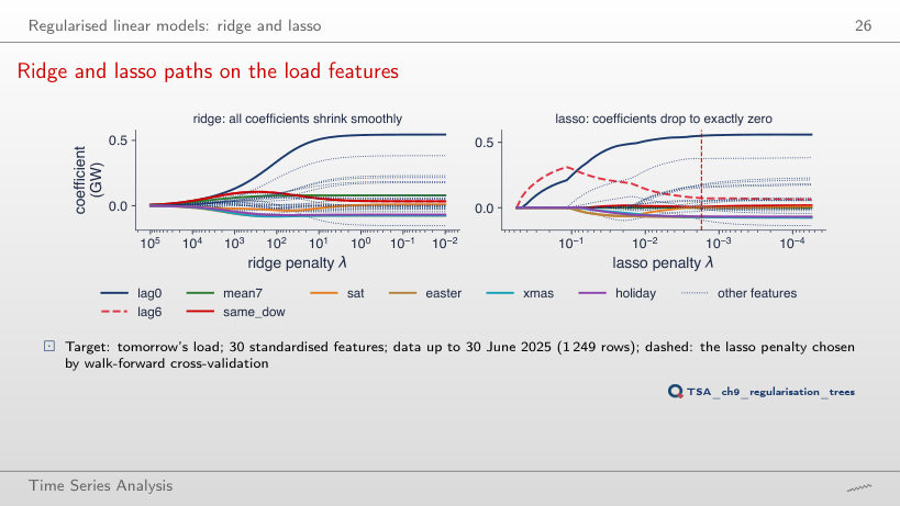
                              Ridge and lasso paths on the load features
                              Slide 26: Ridge and lasso paths on the load features
                              Slide 26
                                Question for the room Cut the sample at 31 December 2023. How many features does the lasso keep at the chosen penalty?
                                Answer

                                23 of 30 (22 on the data up to 30 June 2025), on 702 rows, with λ = 0.00486; the first features to enter are still lag6, lag0 and lag13.

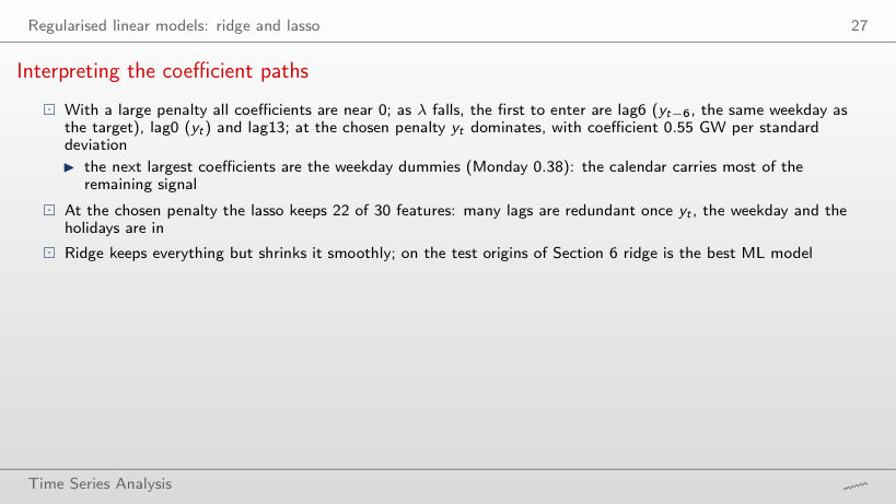
                                Interpreting the coefficient paths
                                Slide 27: Interpreting the coefficient paths
                                Slide 27
                                  Question for the room Move the penalty 6 grid steps towards a larger λ (−6). How many features remain non-zero?
                                  Answer

                                  19 of 30, at λ = 0.00441 (22 at the chosen λ, 0.00173). The order of entry does not depend on the chosen λ: lag6, lag0, lag13.

                                  Trees, random forest and gradient boosting

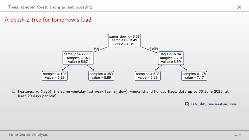
                                  A depth-2 tree for tomorrow's load
                                  Slide 30: A depth-2 tree for tomorrow's load
                                  Slide 30
                                    Question for the room Train the tree on the data up to 29 June 2026. Does the first question change?
                                    Answer

                                    The feature stays same_dow and the threshold falls from 6.08 to 6.04 GW; the leaves become 5.27, 5.86, 6.37 and 7.17 GW, with 1613 days, and R² stays 0.64.

                                    Gradient boosting
                                    Slide 33: Gradient boosting
                                    Slide 33

                                    Worked example

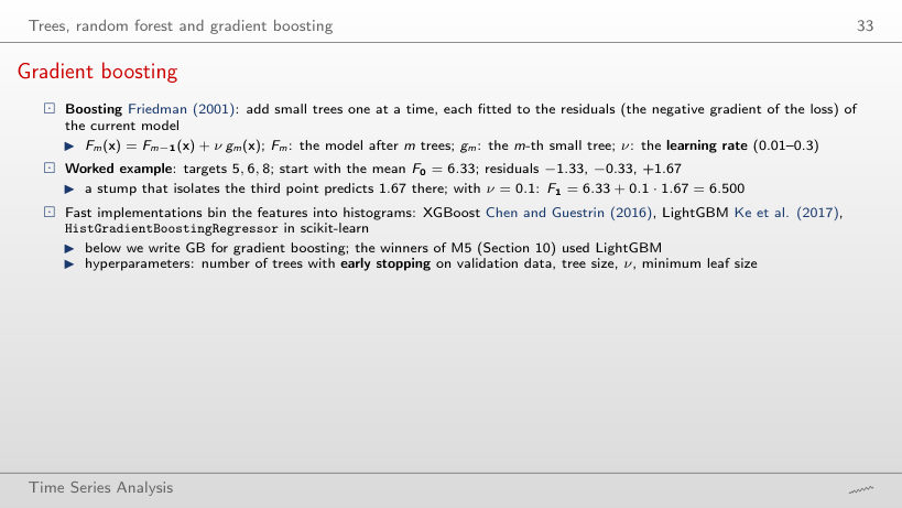
                                    \[F_0=\bar y,\qquad r_i=y_i-F_{m-1}(x_i),\qquad F_m(x)=F_{m-1}(x)+\nu\,g_m(x)\]
                                        Question for the room Set ν = 1. What is F1 at the three points?
                                        Answer

                                        5.50, 5.50 and 8.00: the first tree fully corrects the residual of the isolated point, and the training MSE falls from 1.56 to 0.167 after one tree. A large learning rate fits the training data fast, noise included.

                                        One tree, a forest and boosting on the load
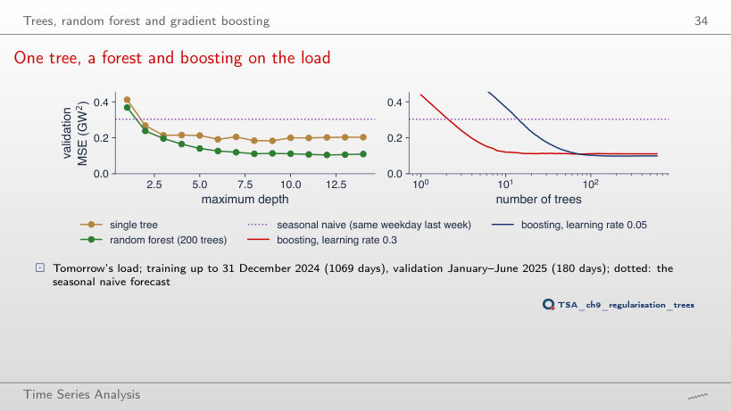
                                        Slide 34: One tree, a forest and boosting on the load
                                        Slide 34
                                          Question for the room Train up to 31 December 2023 (546 validation days). After how many trees does boosting with ν = 0.3 reach its minimum?
                                          Answer

                                          After 24 trees (MSE 0.093), against 72 in the lecture; with ν = 0.05 the minimum comes after 222 trees (0.092). On a shorter training sample fast boosting starts fitting noise earlier.

                                          Trees cannot extrapolate: the Romanian price level
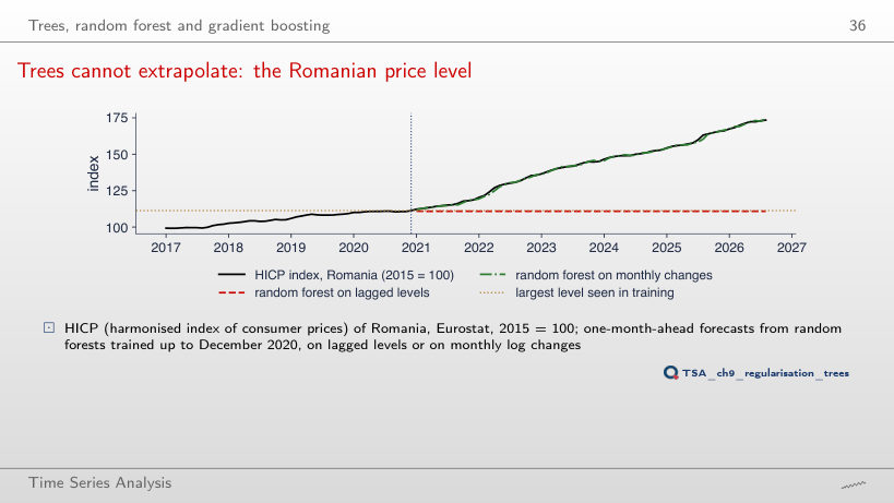
                                          Slide 36: Trees cannot extrapolate: the Romanian price level
                                          Slide 36
                                            Question for the room Train the forests up to December 2022. What is the RMSE on levels?
                                            Answer

                                            22.9 index points (36.9 with training up to 2020): the largest level seen is now 135.6, but the forecast stays capped at 134.1 while the index reaches 173.4. On monthly changes the RMSE is 0.68.

                                            Permutation importance of gradient boosting
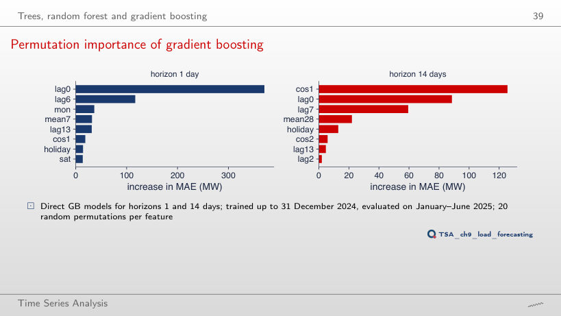
                                            Slide 39: Permutation importance of gradient boosting
                                            Slide 39
                                              Question for the room Move the horizons to 7 and 8 days. Which feature dominates at h = 8?
                                              Answer

                                              cos1 (+98 MW), followed by lag6 (+84 MW). At h = 7 lag0 still dominates (+317 MW), because at 7 days yt is the same weekday as the target.

                                              Neural networks

                                              A small network and its activation functions
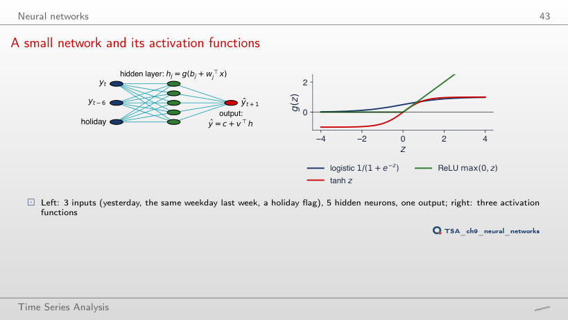
                                              Slide 43: A small network and its activation functions
                                              Slide 43
                                                Question for the room How many parameters does the network with q = 10 hidden neurons have?
                                                Answer

                                                3·10 + 10 + 10 + 1 = 51. With 10 ReLU neurons the piecewise-linear function approximates tanh with maximum error 0.048, against 0.102 with 5.

                                                A recurrent network and the LSTM cell
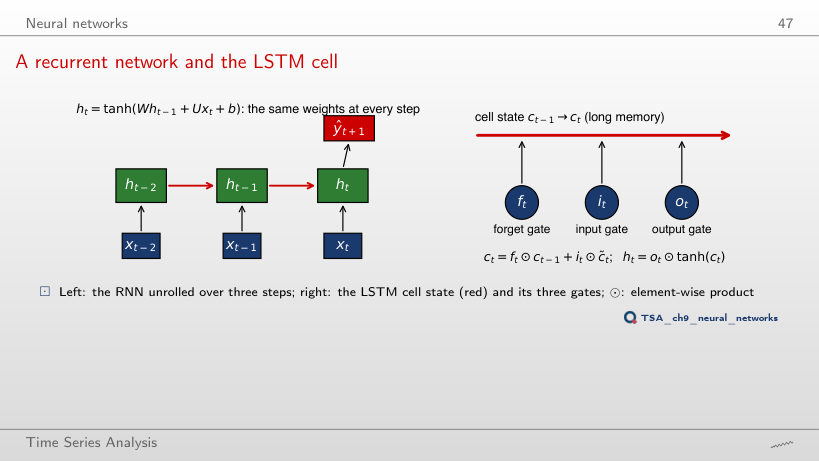
                                                Slide 47: A recurrent network and the LSTM cell
                                                Slide 47
                                                  Question for the room Choose the origin 6 April 2026. What is the MAE of the LSTM, against DHR?
                                                  Answer

                                                  661 MW against 344 MW. The LSTM sees no holiday flag and repeats the weekly pattern over Easter, although its training loss falls from 0.951 to 0.210.

                                                  Application: electricity load against Chapter 4

                                                  The forecasting exercise
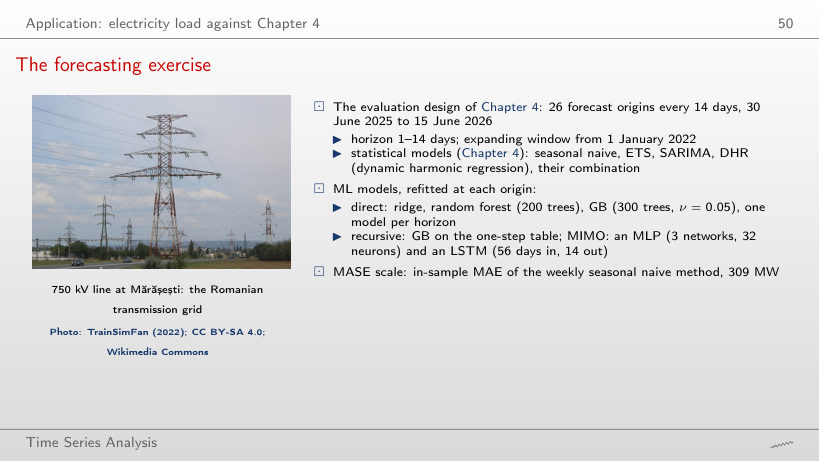
                                                  Slide 50: The forecasting exercise
                                                  Slide 50

                                                  Worked example

                                                  \[\text{MASE}=\frac{\text{MAE}}{\frac{1}{n-m}\sum_{t=m+1}^{n}|y_t-y_{t-m}|}\]
                                                      Question for the room Change the period of the scale to m = 1. What do the scale and the MASE of DHR become?
                                                      Answer

                                                      The scale becomes 371 MW and the MASE 0.744 (309 MW and 0.894 with m = 7). Day-to-day differences are larger than week-to-week ones, because the step into the weekend changes the load; the scale moves the level, not the ranking of the models.

                                                      Results: 26 origins, 14 horizons
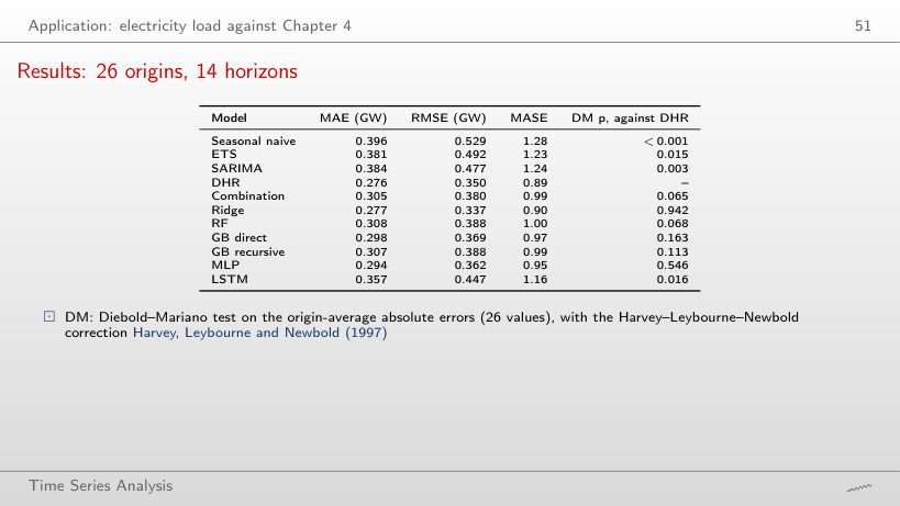
                                                      Slide 51: Results: 26 origins, 14 horizons
                                                      Slide 51
                                                        Question for the room Drop the first 10 origins. Does the difference between ridge and DHR stay not significant?
                                                        Answer

                                                        Yes: on 16 origins ridge has MASE 0.92 and DHR 0.93, and DM p = 0.791. Not significant means that the test does not separate the difference from noise, not that the models are equal.

                                                        MASE and accuracy by horizon
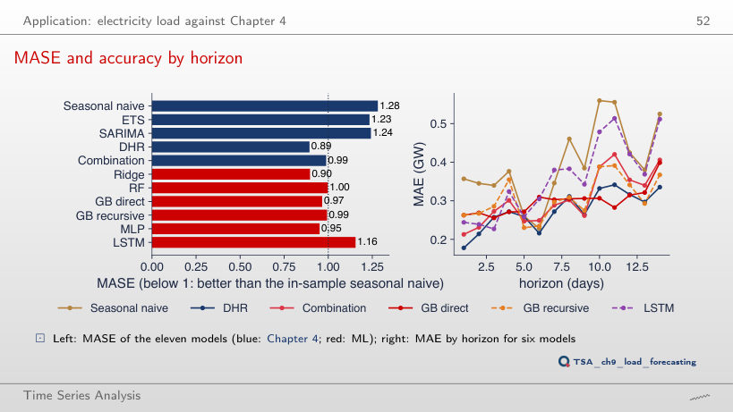
                                                        Slide 52: MASE and accuracy by horizon
                                                        Slide 52
                                                          Question for the room Use only the first 10 origins (up to 3 November 2025). Which model has the lowest MASE?
                                                          Answer

                                                          Still DHR (0.83), followed by ridge (0.86). The LSTM has 0.95 here, but over all 26 origins it rises to 1.16.

                                                          Interpreting the load results
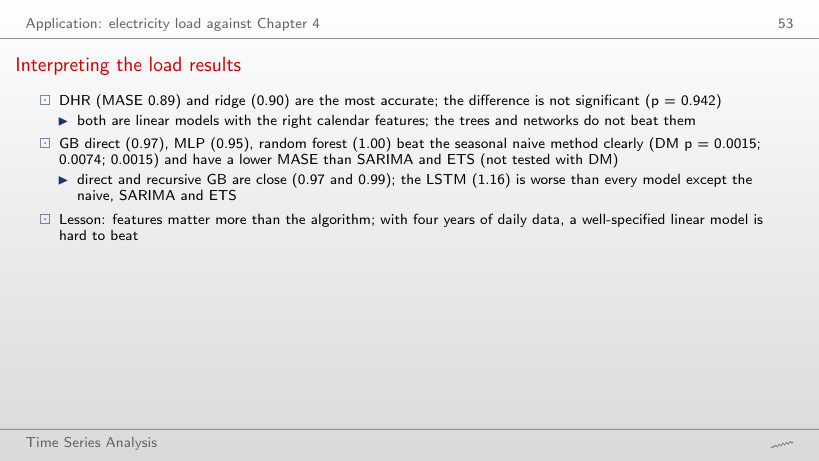
                                                          Slide 53: Interpreting the load results
                                                          Slide 53

                                                          Worked example

                                                          \[d_t=\overline{|e|}_{t}^{\,A}-\overline{|e|}_{t}^{\,B},\quad \hat V=\frac{1}{n}\Big(\hat\gamma_0+2\sum_{k=1}^{h-1}\hat\gamma_k\Big),\quad DM=\frac{\bar d}{\sqrt{\hat V}},\quad DM^{*}=c_h\,DM\sim t_{n-1}\]
                                                              Question for the room Include 2 autocovariances (h = 3) for ridge against DHR. What does p become?
                                                              Answer

                                                              0.953 (DM* = 0.060), against 0.942 without autocovariances: d̄ = 0.9 MW is small relative to its standard error, however the variance is estimated.

                                                              Forecasts around Orthodox Easter 2026
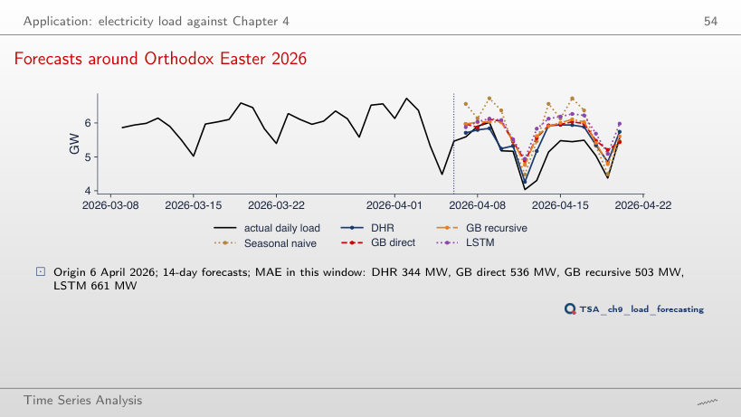
                                                              Slide 54: Forecasts around Orthodox Easter 2026
                                                              Slide 54
                                                                Question for the room Choose the origin 20 April 2026, after Easter. Which model has the lowest MAE?
                                                                Answer

                                                                The MLP, with 255 MW; GB recursive has 260, GB direct 276, the seasonal naive 283, DHR 286 and the LSTM 398 MW. Without Easter in the window the differences between the models are small.

                                                                Prediction intervals

                                                                Quantile regression and the pinball loss
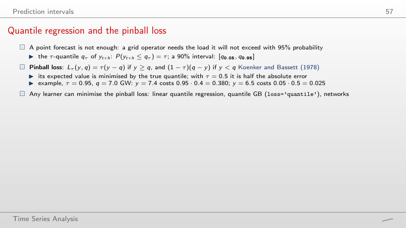
                                                                Slide 57: Quantile regression and the pinball loss
                                                                Slide 57

                                                                Worked example

                                                                \[L_\tau(y,q)=\begin{cases}\tau\,(y-q), & y\ge q\\(1-\tau)\,(q-y), & y
                                                                    Question for the room Set τ = 0.5. What do y = 7.4 and y = 6.5 cost for q = 7.0?
                                                                    Answer

                                                                    0.200 and 0.250: with τ = 0.5 the loss is half the absolute error (0.4/2 and 0.5/2), and the minimum of the mean loss moves to the median of the 364 values.

                                                                    Split conformal prediction
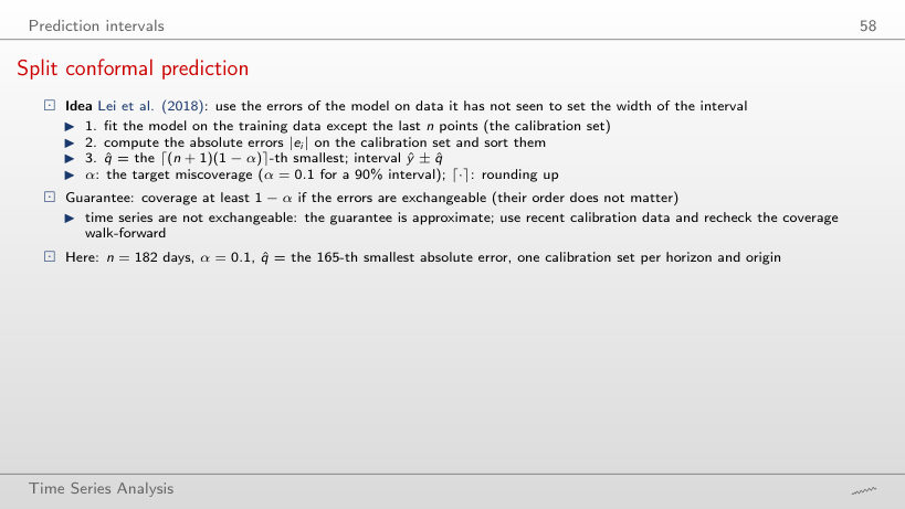
                                                                    Slide 58: Split conformal prediction
                                                                    Slide 58

                                                                    Worked example

                                                                    \[k=\lceil (n+1)(1-\alpha)\rceil,\qquad \hat q=|e|_{(k)},\qquad \hat y\pm\hat q\]
                                                                        Question for the room Lower the level to 50%. What is k and what coverage does the interval reach?
                                                                        Answer

                                                                        k = ⌈183·0.5⌉ = 92 and q̂ = 175 MW for h = 1; the coverage over the 364 forecasts is 49.5%, with mean width 509 MW.

                                                                        90% intervals for the load
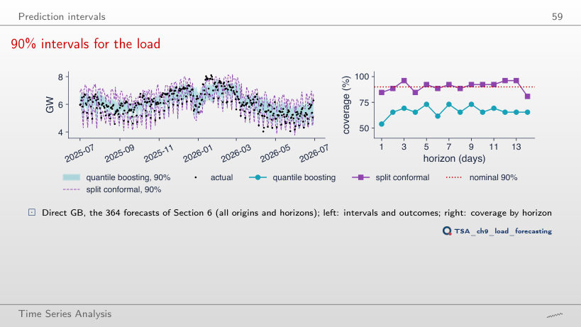
                                                                        Slide 59: 90% intervals for the load
                                                                        Slide 59
                                                                          Question for the room Lower the conformal level to 80%. What coverage does it reach?
                                                                          Answer

                                                                          77.5%, with mean width 1000 MW: 13.7% of the outcomes fall below the interval and 8.8% above. Quantile GB stays at 66.5% for a nominal 90%.

                                                                          Local and global models: Romanian inflation

                                                                          Romanian inflation: forecasts and relative RMSE
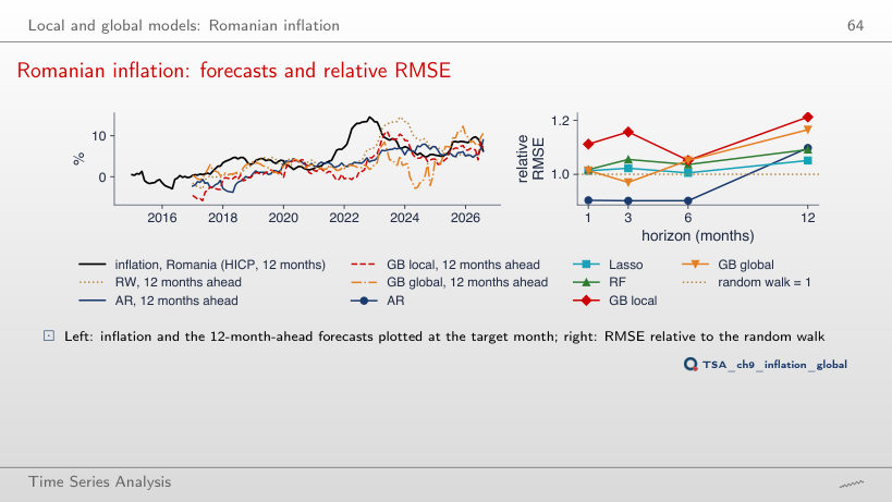
                                                                          Slide 64: Romanian inflation: forecasts and relative RMSE
                                                                          Slide 64
                                                                            Question for the room Start the test origins in 2022. What is the relative RMSE of GB local at 12 months?
                                                                            Answer

                                                                            0.64 (1.21 over all origins), while GB global has 1.19. On the few origins of the disinflation after the 2022 peak the 12-month ranking reverses: a comparison on a few dozen errors is fragile.

                                                                            Inflation results
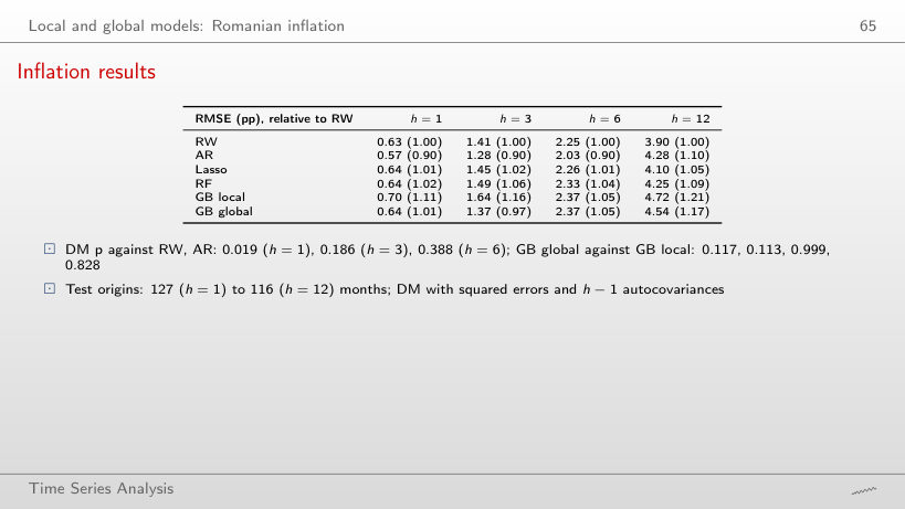
                                                                            Slide 65: Inflation results
                                                                            Slide 65
                                                                              Question for the room Choose the origins of 2021–2023. What is the relative RMSE of the AR at h = 6?
                                                                              Answer

                                                                              0.83 (0.88, 0.86, 0.83 and 0.98 at h = 1, 3, 6, 12): in the high-inflation years the AR stays below the random walk up to 6 months, while GB global has 1.10 at h = 6.

                                                                              Applications in finance: volatility and the sign of returns

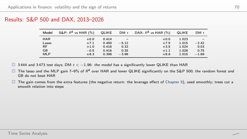
                                                                              Results: S&P 500 and DAX, 2013–2026
                                                                              Slide 70: Results: S&P 500 and DAX, 2013–2026
                                                                              Slide 70
                                                                                Question for the room Start the test period in 2020. Is the lasso still significantly more accurate than HAR on the S&P 500?
                                                                                Answer

                                                                                Yes: R² against HAR +7.4% and DM t = −3.42 on 1682 days; the MLP has +7.9% and t = −2.28.

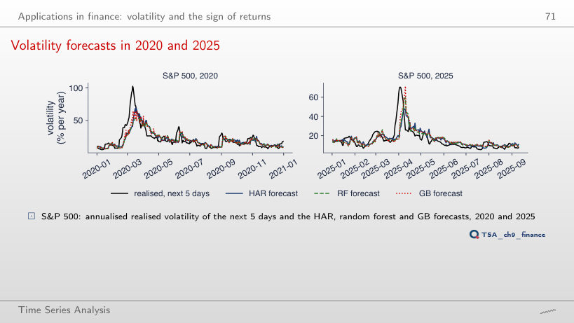
                                                                                Volatility forecasts in 2020 and 2025
                                                                                Slide 71: Volatility forecasts in 2020 and 2025
                                                                                Slide 71
                                                                                  Question for the room Show the lasso and the MLP for the S&P 500 in 2022 (left year). Does either beat HAR by QLIKE in that year?
                                                                                  Answer

                                                                                  Yes, both: QLIKE 1.536 (lasso) and 1.541 (MLP), against 1.553 for HAR. In 2025 HAR has 0.990, below both (0.997 and 1.002): one year does not decide the ranking.

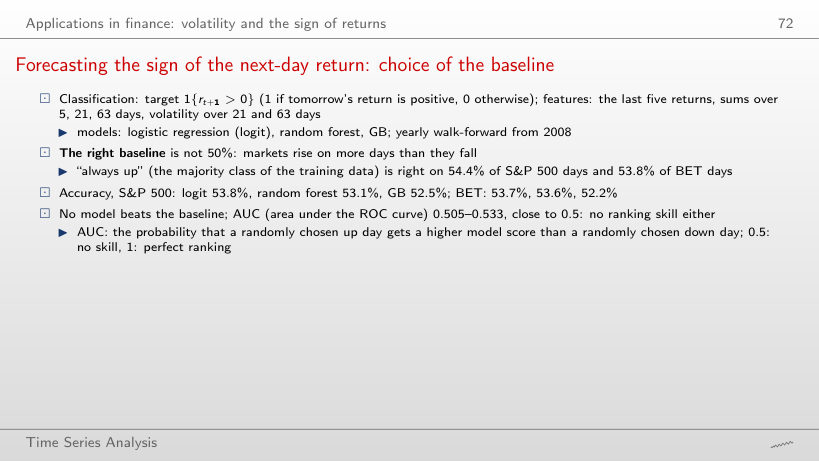
                                                                                  Forecasting the sign of the next-day return: choice of the baseline
                                                                                  Slide 72: Forecasting the sign of the next-day return: choice of the baseline
                                                                                  Slide 72
                                                                                    Question for the room Start the test period in 2016. What is the largest AUC?
                                                                                    Answer

                                                                                    0.541, the smallest 0.507; the up days are 54.6% (S&P 500) and 55.7% (BET). AUC stays close to 0.5.

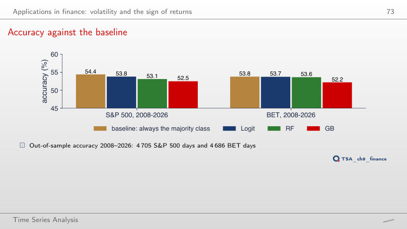
                                                                                    Accuracy against the baseline
                                                                                    Slide 73: Accuracy against the baseline
                                                                                    Slide 73
                                                                                      Question for the room Raise the threshold to 0.55. What accuracy does GB reach on the S&P 500?
                                                                                      Answer

                                                                                      49.3%, below the 54.4% baseline: with the higher threshold the model forecasts “up” on only 40.4% of the days, while the market rises on 54.4% of them.

                                                                                      Landmark case studies: M4, M5 and Gu, Kelly and Xiu

                                                                                      M4: the accuracy of all methods
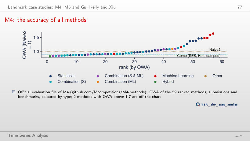
                                                                                      Slide 77: M4: the accuracy of all methods
                                                                                      Slide 77
                                                                                        Question for the room Set the weight of sMAPE to 1 (OWA from sMAPE only). Where does Comb rank?
                                                                                        Answer

                                                                                        23rd (OWA 0.926), against 19th; the winner is still method 118, a hybrid, with 0.839, and the best pure ML method falls to rank 27.

                                                                                        Gu, Kelly and Xiu (2020): out-of-sample R² and Sharpe ratios
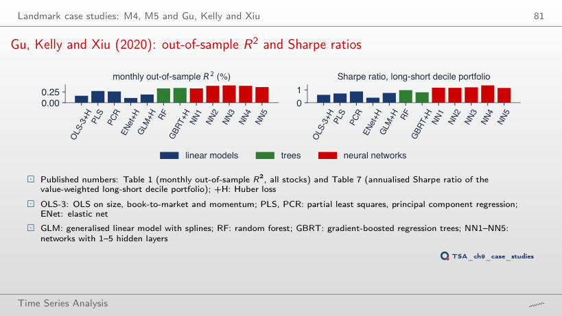
                                                                                        Slide 81: Gu, Kelly and Xiu (2020): out-of-sample R² and Sharpe ratios
                                                                                        Slide 81
                                                                                          Question for the room How many times larger is the Sharpe ratio of NN4 than that of OLS-3+H?
                                                                                          Answer

                                                                                          1.35/0.61 = 2.21 times, with a monthly R² of only 0.39%: a small predictability, used on thousands of stocks and months, supports a valuable portfolio.

                                                                                          Daily mean electricity load of Romania (ENTSO-E, the extract of Chapter 4, 1 January 2022 – 30 June 2026). Daily S&P 500, DAX and BET prices (data/market, up to 18 September 2026). The Romanian HICP index (Eurostat prc_hicp_minr), read with the chapter’s loader on 4 November 2026 and cut at August 2026, the last month of the slides; it reproduces the numbers of the lecture exactly. The official M4 evaluation file (ch9_m4_owa.csv) and the published numbers of Gu, Kelly and Xiu (2020). The walk-forward forecasts of the models (ch9_load_ml.csv, ch9_inflation.csv, ch4_load_cv.csv) and the estimates that need the models to be retrained (random forest, gradient boosting, MLP, LSTM, lasso) are those of the chapter code, with the same seed; the browser recomputes the lag tables, the correlations, the regression trees, MASE, the Diebold–Mariano tests, the coverage of the intervals, RMSE, QLIKE, accuracy and AUC. Variants that do not appear in the lecture (another horizon, another noise level, another sample end, another interval level, another threshold) are extra runs of the chapter code with the same data and seed; the AR(1) models of the strategies block and the approximation of tanh by ReLU neurons are extra computations made in the browser.