Bucharest University of Economic Studies IDA Institute Digital Assets Blockchain Research Center AI4EFin Artificial Intelligence for Energy Finance Romanian Academy, Institute for Economic Forecasting MSCA Digital Finance
The chapter's question has two parts: which cycles a series contains, and how much of its variance each cycle explains. The first part concerns the location of the cycles, that is, their frequency or period; the second concerns their importance. A cycle can be present and still negligible if it explains a small part of the variation of the series. The chapter's three examples cover very different time scales: the 11-year sunspot cycle, the business cycle of a few years, and the daily and weekly rhythm of electricity demand.
The route starts from a single cycle and from the discrete Fourier transform, which rewrites any series as a sum of cycles. Next comes the spectral density, the theoretical version of this decomposition for stationary processes, computed for white noise and for ARMA models. The periodogram is its direct estimator; its weaknesses, above all the fact that it does not become more precise with more data, motivate smoothing and confidence bands. The last sections apply the tools to real data and extend them to long memory, to filters, to pairs of series and, briefly, to wavelets.
In brief
Question: which cycles does a series contain, and how much of its variance does each cycle explain?
examples: the 11-year sunspot cycle, the business cycle, the daily and weekly rhythm of electricity demand
Route of the chapter
cycles, frequencies and the discrete Fourier transform
the spectral density of white noise and of ARMA models
the periodogram, its weaknesses, and how to smooth it
cycles in data; long memory; filters; two series; wavelets as a pointer
Self-study chapter: worked examples, interpretation slides and a recap after each section; self-assessment with answers at the end
The first group of outcomes concerns the language of frequency. A frequency \(\nu\), measured in cycles per observation, corresponds to a period of \(1/\nu\) observations and to an angular frequency of \(2\pi\nu\) radians per observation; a sample of length \(T\) has the Fourier frequencies \(j/T\). On this basis one computes the spectral density of simple models, AR(1), MA(1) and AR(2), and reads its shape as a description of dependence: flat, decreasing, increasing or with a peak.
The second group is statistical. The periodogram of a short series can be computed by hand, and the distribution of its ordinates explains why the raw estimator stays noisy however long the sample. Tapering the ends of the series, smoothing with the Daniell, Bartlett or Welch methods, and confidence bands based on the chi-square distribution turn the periodogram into a usable estimator. The third group is empirical: identifying cycles in sunspots, GDP and electricity load, and reading the coherence and phase between two series.
In brief
Convert between frequency, period and angular frequency, and find the Fourier frequencies of a sample
Compute the spectral density of white noise, AR(1), MA(1) and AR(2) models and read its shape
Compute a periodogram by hand for a short series and explain why the raw periodogram is not consistent
Smooth the periodogram (Daniell, Bartlett, Welch), taper the data and build chi-square confidence bands
Identify cycles in sunspots, GDP and electricity load; read coherence and phase between two series
The main reference is Shumway and Stoffer (2017), chapter 4, which treats spectral analysis and filtering at a level suited to this course. For theory, Brockwell and Davis (1991) give the proofs in chapters 4 and 10 of the book, and Hamilton (1994) presents spectral analysis from the econometric point of view in chapter 6. Huang and Petukhina (2022) show the applications in Python.
One difference in notation must be kept in mind. Shumway and Stoffer (2017) measure the frequency \(\nu\) in cycles per observation, the convention used here as well, whereas in Chapter 8 long memory was written with the angular frequency \(\lambda = 2\pi\nu\), in radians per observation. Formulas move from one convention to the other through the substitution \(\lambda = 2\pi\nu\), and the interval \([0, \pi]\) of angular frequency corresponds to the interval \([0, 1/2]\) of \(\nu\).
The chapter's code writes the periodogram, Daniell smoothing and the Morlet wavelet explicitly in numpy, so that every step of the computation is visible; the Welch estimate and the coherence use the functions of scipy.signal. The course notebook reproduces the chapter's computations and charts.
The previous chapters described time series through autocorrelations: how strongly today's value is related to yesterday's, to last month's or to last year's. Many series, however, have a structure that is more naturally described by cycles. The number of sunspots rises and falls about every 11 years, output goes through expansions and recessions, and electricity demand repeats the same pattern every day and every week. Spectral analysis asks the question directly: which cycles does a series contain, and what share of its variance does each cycle explain?
The answer is the spectral density, a function that splits the variance of the series across frequencies. It contains the same information as the autocovariance function but shows it differently: a cycle that appears in the autocorrelations as a damped wave, hard to read, becomes in the spectrum a peak at a precise frequency. The chapter defines the spectrum, computes it for autoregressive moving average (ARMA) models, estimates it from data with the periodogram and its smoothed versions, and applies it to the sunspots, to the gross domestic product (GDP) of the United States and of Romania, to Romania's hourly electricity load and to the returns of the S&P 500 index.
The empirical results are clear in some cases and cautious in others. The sunspot cycle appears as a peak at 11.0 years, and Fisher's test rejects white noise with a p-value below 0.001. The daily cycle and its harmonics explain 34% of the variance of electricity load. The US GDP cycle extracted with the Hodrick–Prescott (HP) filter has 80% of its variance in the business-cycle band, with a peak at about 6.1 years, while Romania's 99 observations are too few for a clear answer.
The yearly mean sunspot number, 1700–2008, 309 observations (Wolf / SILSO series, Sunspot Index and Long-term Solar Observations), and its raw periodogram, with the main peak at a period of 11.0 years.
What you will be able to do
Move between frequency, period and angular frequency, and find the Fourier frequencies of a sample.
Compute the spectral density of white noise and of AR(1), MA(1) and AR(2) models, and interpret its shape.
Compute the periodogram of a short series by hand and explain why the raw periodogram is not a consistent estimator.
Estimate the spectrum by tapering and smoothing (Daniell, Bartlett, Welch) and build chi-square confidence bands.
Interpret the cycles in sunspots, GDP and electricity load, long memory, the gain of a filter, and the coherence and phase between two series.
Chapter plan
Cycles and frequenciesAmplitude, frequency and phase; Fourier frequencies, the discrete Fourier transform, Parseval's theorem and aliasing.
The spectral densityThe spectrum as a transform of the autocovariances; white noise, AR(1), MA(1), ARMA and the pseudo-cycles of an AR(2).
The periodogramThe basic estimator, the sunspots, the chi-square distribution of the ordinates and Fisher's test.
Estimating the spectrumLeakage and tapering, Daniell smoothing, lag windows, Welch's method and confidence bands.
SummaryKey ideas, formulas and self-assessment questions.
Cycles and frequencies
The section introduces the basic language of spectral analysis: a pure cycle and its parameters, the Fourier frequencies of a sample, the discrete Fourier transform, which rewrites the data as a sum of cycles, and the limit imposed by observing at discrete intervals, aliasing.
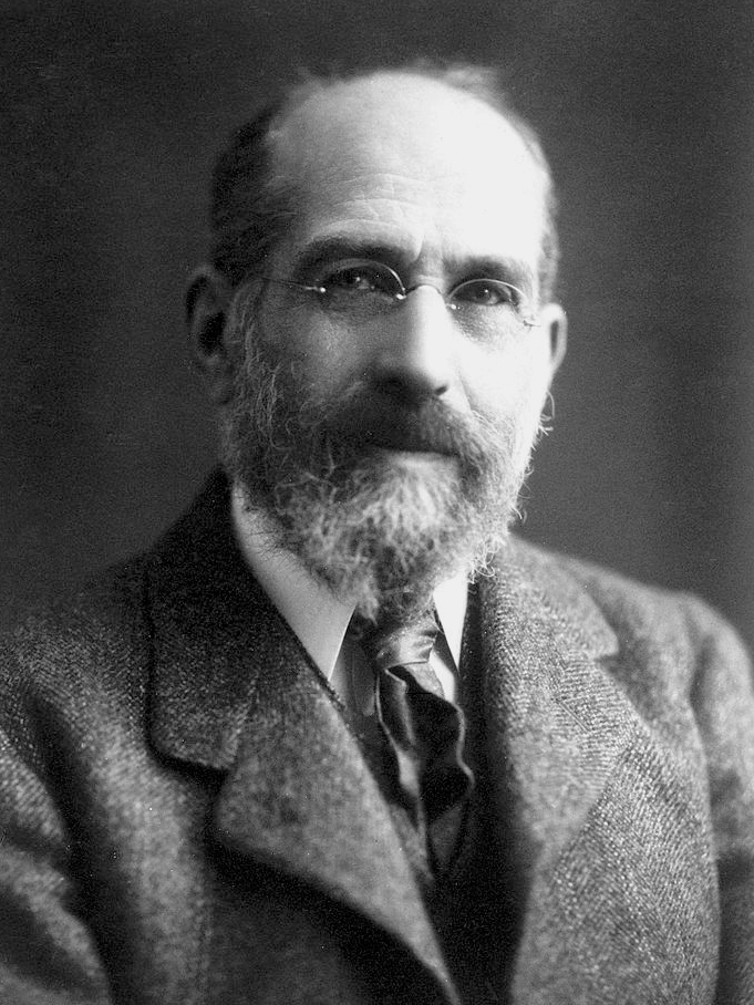
Joseph Fourier studied, at the beginning of the nineteenth century, the propagation of heat in a solid body. To solve this problem he wrote the temperature as a sum of sines and cosines, each with its own frequency and amplitude. The idea became one of the most widely used tools of applied mathematics: a complicated function is decomposed into pure cycles, and each cycle is studied separately.
Applied to a time series, the idea becomes a statistical question: what part of the variance of the series lies at each frequency? Chapters 1–8 described a stationary series in the time domain, through the autocorrelation function (ACF). The frequency domain describes the same series through the spectrum.
The two descriptions are mathematically equivalent, as the second section will show, but they are not equally easy to read. An 11-year cycle appears in the ACF as a damped wave stretching over dozens of lags, mixed with the other components of the series; in the spectrum the same cycle is a single peak, whose position gives the period and whose area gives the share of the variance.
The simplest object of spectral analysis is the pure cycle \(x_t = A\cos(2\pi\nu t + \varphi)\). The amplitude \(A\) is the height of the wave, the phase \(\varphi\) fixes where the wave is at \(t = 0\), and the frequency \(\nu\) says what fraction of a cycle is covered from one observation to the next. The period \(1/\nu\) is the number of observations in one complete cycle. The angular frequency \(\omega = 2\pi\nu\) measures the same thing in radians per observation.
Frequency has no meaning without the time unit of the data. For monthly data, a yearly cycle has \(\nu = 1/12\) cycles per month. For hourly data, the daily cycle has \(\nu = 1/24\), and for quarterly data a 6-year cycle also has \(\nu = 1/24\): the same frequency per observation can describe completely different phenomena. Every spectral result must therefore be translated at the end into periods expressed in concrete time units.
The form \(a\cos(2\pi\nu t) + b\sin(2\pi\nu t)\), with \(a = A\cos\varphi\) and \(b = -A\sin\varphi\), follows from the formula for the cosine of a sum. It is useful because, for a given frequency, it is linear in \(a\) and \(b\): the amplitude and phase of a cycle of known frequency are estimated by an ordinary least squares (OLS) regression on a cosine and a sine, and \(A = \sqrt{a^2 + b^2}\). The highest frequency that can be observed in discrete data is \(\nu = 1/2\), one cycle every two observations, called the Nyquist frequency.
In brief
A pure cycle: \(x_t = A\cos(2\pi\nu t + \varphi)\), \(t = 1, 2, \ldots\)
\(A\): amplitude (height of the wave); \(\varphi\): phase (where the wave starts)
\(\nu\): frequency, in cycles per observation; the period\(1/\nu\) is the number of observations per cycle
angular frequency \(\omega = 2\pi\nu\), in radians per observation
Example: monthly data with an annual cycle: \(\nu = 1/12\) cycles per month, period 12 months
hourly data with a daily cycle: \(\nu = 1/24\); quarterly data with a 6-year cycle: \(\nu = 1/24\) as well
Question for the room Set φ = 1.5 radians, with A = 2. What are a and b?
Answer
a = 2 cos 1.5 = 0.14 and b = −2 sin 1.5 = −1.99: with a phase close to π/2 the cycle is almost a pure sine with a negative sign. Whatever the phase, a² + b² = 4 = A².
Question for the room ▶ moves x₃. With x = (4, 2, 4, 2), where does the variance sit?
Answer
All at ν = 1/2: the deviations (1, −1, 1, −1) alternate, so |d(1/2)|² = (−4)²/4 = 4 and |d(1/4)|² = |d(3/4)|² = 0; Parseval: 4 = 1 + 1 + 1 + 1. The series has period 2.
Question for the room Set the amplitude of the period-4 cycle to 2, as large as the annual cycle. How high is the spike at ν = 1/4 now?
Answer
119.2, four times higher than with amplitude 1 (29.6) and close to the theory A²T/4 = 4·120/4 = 120: the spike grows with the square of the amplitude. The spike at 1/12 stays at 139.7, above its theoretical 120, because the noise also contributes at that frequency; without noise the two spikes are exactly 120 and 30.
The simulated series has 120 observations and combines two cycles: one with period 12 and amplitude 2, and one with period 4, amplitude 1 and phase 1. On top of them comes Normal white noise with variance 0.49. If the observations were monthly, the first cycle would be yearly and the second would last four months.
The left panel shows the series in the time domain. The 12-period cycle can be vaguely recognised as an alternation of high and low values, but the 4-period cycle and the noise are superimposed on it. The right panel shows the periodogram of the same series, that is, at each Fourier frequency, a quantity proportional to the squared amplitude of the best-fitting cycle; the exact definition comes in the third section. The horizontal axis is frequency, from 0 to the Nyquist frequency 1/2.
In brief
Simulated series, \(T = 120\): \(x_t = 2\cos(2\pi t/12) + \cos(2\pi t/4 + 1) + \varepsilon_t\), \(\varepsilon_t \sim N(0, 0.49)\) (Normal white noise with variance 0.49); right: its periodogram (defined in Section 3)
In the frequency domain the two cycles are completely separated: they appear as two isolated peaks, at \(\nu = 1/12\) and at \(\nu = 1/4\), and the rest of the periodogram is low and almost flat. The observed heights of the peaks are 139.7 and 29.6. For a cycle of amplitude \(A\) located exactly at a Fourier frequency, the theoretical height is \(A^2T/4\), that is \(4 \cdot 120/4 = 120\) for the first cycle and \(1 \cdot 120/4 = 30\) for the second. The differences from theory come from the noise, which adds or subtracts a little at every frequency.
The ratio of the peaks shows that the periodogram measures power, not amplitude. The first cycle has twice the amplitude, and its peak is four times higher. Together, the two peaks hold 85% of the total power of the series; white noise spreads the rest evenly over all frequencies, so that no single frequency receives a large share. This is, in miniature, the idea of the whole chapter: a cycle concentrates variance at one frequency, noise spreads it over all of them.
In brief
In the time domain the two cycles are hard to separate by eye
in the frequency domain they are two isolated spikes, at \(\nu = 1/12\) and \(\nu = 1/4\)
Height of the spikes: 139.7 and 29.6; theory for a cycle of amplitude \(A\) at a Fourier frequency: \(A^2T/4\), i.e. 120 and 30
the spike grows with the squared amplitude: the larger cycle dominates
The two spikes hold 85% of the total power; the noise spreads the rest evenly over all frequencies
Fourier frequencies and the discrete Fourier transform (1/2)
A sample of \(T\) observations cannot distinguish every frequency. The natural frequencies of the sample are the Fourier frequencies \(\nu_j = j/T\), for \(j = 0, 1, \ldots, \lfloor T/2 \rfloor\): the cycles that fit exactly \(j\) times into the sample. For \(T = 120\) monthly observations, \(j = 10\) gives \(\nu = 1/12\), the yearly cycle, which fits ten times; \(j = 1\) gives a single cycle over the whole sample, the slowest cycle that can be observed completely.
The discrete Fourier transform (DFT) measures, at each Fourier frequency, how strongly the series moves together with a cycle of that frequency:
\[d(\nu_j) = T^{-1/2}\sum_{t=1}^{T} x_t\, e^{-2\pi i \nu_j t}.\]
(12.1)
Euler's formula, \(e^{-i\theta} = \cos\theta - i\sin\theta\), shows what the complex exponential does: the real part of \(d(\nu_j)\) is, up to the factor \(T^{-1/2}\), the inner product of the series with a cosine, and the imaginary part, with its sign changed, the inner product with a sine of the same frequency. A large inner product means that the series and the wave rise and fall together.
Complex numbers are here only a compact notation. Both correlations, with the cosine and with the sine, are needed because the cycle in the data can have any phase: a cosine alone would miss a cycle shifted by a quarter of a period. The squared modulus \(|d(\nu_j)|^2 = (\mathrm{Re}\,d)^2 + (\mathrm{Im}\,d)^2\) adds the two contributions and no longer depends on the phase.
In brief
For a sample \(x_1, \ldots, x_T\), the Fourier frequencies are \(\nu_j = j/T\), \(j = 0, 1, \ldots, \lfloor T/2 \rfloor\)
cycles that fit an integer number of times (\(j\) times) in the sample; \(\lfloor T/2 \rfloor\): the integer part of \(T/2\)
The discrete Fourier transform (DFT) measures how strongly the series moves with a cycle of frequency \(\nu_j\)
\(d(\nu_j) = T^{-1/2}\sum_{t=1}^{T} x_t\, e^{-2\pi i \nu_j t}\)
\(i\): the imaginary unit, \(i^2 = -1\); \(e^{-i\theta} = \cos\theta - i\sin\theta\) (Euler's formula)
so the DFT correlates the series with a cosine (real part) and a sine (imaginary part) of frequency \(\nu_j\)
Fourier frequencies and the discrete Fourier transform (2/2)
The \(T\) values \(d(\nu_j)\), for \(j = 0, \ldots, T-1\), contain exactly the same information as the \(T\) observations: the inverse transform recovers the series without any loss. The DFT is therefore a change of coordinates, not an approximation. The series is written as a sum of cycles at the Fourier frequencies, and \(d(\nu_j)\) gives the coefficient of each cycle.
Parseval's theorem says that this change of coordinates also preserves the sum of squares:
On the left is the sum of squared deviations from the sample mean \(\bar x\), that is \(T\) times the sample variance; on the right, the sum of squared moduli of the DFT at all non-zero frequencies. Frequency zero is missing because \(d(0)\) is proportional to the mean, which has been subtracted. The interpretation is central to the whole chapter: the variance of the series splits exactly across frequencies, and each \(|d(\nu_j)|^2\) is the contribution of the cycle of frequency \(\nu_j\).
Computing all \(T\) values directly takes a number of operations of order \(T^2\), since each value is a sum of \(T\) terms. The fast Fourier transform (FFT) of Cooley and Tukey (1965) reduces the cost to order \(T\log T\) by splitting the sum recursively into smaller sums. For the long series of this chapter, for example tens of thousands of hours of electricity load, the difference turns a slow computation into an instantaneous one.
In brief
The \(T\) values \(d(\nu_j)\) contain exactly the same information as the \(T\) data points
the data can be recovered from them by the inverse transform
Parseval
the sum of squared deviations equals the sum of the squared moduli of the DFT
The example uses four observations, \(x = (4, 2, 0, 2)\), with mean 2 and deviations \(y = (2, 0, -2, 0)\). With \(T = 4\), the non-zero Fourier frequencies up to Nyquist are \(\nu_1 = 1/4\), a cycle of period 4 that fits once into the sample, and \(\nu_2 = 1/2\), a cycle of period 2. The deviations go up, down and back in a single wave, so all the variation should lie at period 4.
At \(\nu = 1/4\), the exponential \(e^{-i\pi t/2}\) takes the values \(-i\),\(-1\),\(i\) and \(1\) for \(t = 1, 2, 3, 4\). Only \(t = 1\) and \(t = 3\) have non-zero deviations, so the sum is \(2(-i) + (-2)(i) = -4i\), and dividing by \(\sqrt 4 = 2\) gives \(d(1/4) = -2i\), with \(|d(1/4)|^2 = 4\). At \(\nu = 1/2\), the exponential is \((-1)^t\), and the sum \(-2 + 2 = 0\): the series has no component of period 2. The value at \(\nu = 3/4\) is the conjugate of the one at \(1/4\) and has the same squared modulus, 4.
The check with (12.2):\(4 + 0 + 4 = 8\), equal to the sum of squared deviations, \(2^2 + 0^2 + (-2)^2 + 0^2 = 8\). Divided by \(T = 4\), this gives the sample variance 2, located entirely at period 4. The line of code on the slide does the same computation with the FFT and returns the vector \((0, 4, 0, 4)\) for the frequencies \(0\),\(1/4\),\(1/2\) and \(3/4\).
Question for the room Set the period of the true cycle to 2.5 months, with quarterly observations (Δ = 3). What period does the cycle appear to have?
Answer
15 months: 3/2.5 = 1.2 cycles per quarter, which folds to |1.2 − 1| = 0.2, i.e. 5 quarters. A cycle faster than the observations appears as a slower, false cycle.
Question for the room ▶ changes the sampling interval. At Δ = 4 months (one observation per cycle), what do the observations show?
Answer
A constant: the cycle has 4/4 = 1 cycle per observation, which folds to |1 − 1| = 0, so every observation falls at the same point of the cycle and the 4-month cycle disappears from the data (an alias of infinite period). At Δ = 5 months the same cycle appears as a 20-month cycle.
The chart shows a cycle with a period of 4 months, so with frequency \(\nu = 1/4\) cycles per month, observed only once every three months, as in a quarterly statistic. The continuous curve is the true cycle; the dots are the values recorded each quarter. Between two consecutive dots, the true cycle covers three quarters of a period.
The quarterly dots seem to follow a much slower wave than the true one, and the chart also draws this wave, with a period of 12 months, which passes through the same dots. For someone who sees only the quarterly data, the two waves cannot be told apart.
In brief
A cycle of 4 months (\(\nu = 1/4\) per month) observed only once a quarter (every 3 months)
The explanation is arithmetic. Measured in quarters, the 4-month cycle has frequency \(3 \times 1/4 = 3/4\) cycles per quarter, above the Nyquist frequency 1/2 of quarterly data. A frequency above Nyquist does not disappear; it folds back into the interval \([0, 1/2]\):\(|3/4 - 1| = 1/4\) cycles per quarter, that is a period of 4 quarters or 12 months. The reason is that \(\cos(2\pi \cdot \tfrac34 t)\) and \(\cos(2\pi \cdot \tfrac14 t)\) take the same values for every integer \(t\), because their frequencies differ by one whole cycle per observation.
This is aliasing: a cycle faster than two observations appears in the data as a slower, false cycle. The danger is practical. A quarterly or yearly series built by picking a single value from each period can contain slow cycles that do not exist in reality but come from fast rhythms in the underlying data.
Prevention has two parts. The sampling frequency must be at least twice the frequency of the cycle of interest, that is, each cycle must contain at least two observations. And when aggregating to a lower frequency, for example from months to quarters, take the average of the values in the period rather than picking one of them: averaging dampens the fast cycles before they can fold onto the slow ones.
In brief
Per quarter, the true frequency is \(3 \times 1/4 = 3/4\) cycles, above the Nyquist frequency \(1/2\)
it is folded back to \(|3/4 - 1| = 1/4\) cycles per quarter: a period of 4 quarters, i.e. 12 months
The quarterly points lie exactly on a 12-month wave: the data cannot tell the two cycles apart
this is aliasing: cycles faster than two observations appear as slower, false cycles
Practical rule: sample at least twice per cycle of interest; average (rather than pick) values when you aggregate to a lower frequency
A pure cycle has an amplitude, a frequency in cycles per observation, a period equal to the inverse of the frequency, and a phase. The discrete Fourier transform (12.1) rewrites a sample as a sum of cycles at the Fourier frequencies \(j/T\) without loss of information, and Parseval's theorem (12.2) splits the sum of squared deviations across these frequencies. Discrete data show only frequencies up to 1/2; faster cycles appear as aliases at lower frequencies.
In brief
A cycle has an amplitude, a frequency \(\nu\) (cycles per observation), a period \(1/\nu\) and a phase
The DFT at the Fourier frequencies \(j/T\) rewrites the data as a sum of cycles; Parseval splits the variance by frequency
Only frequencies up to \(1/2\) are visible; faster cycles are aliased
Section summary
The section worked with a given sample: the DFT splits the observed variance across frequencies. Inference needs the corresponding theoretical object, a function that says how the variance of a stationary process is distributed across frequencies. This is the spectral density, directly linked to the autocovariances used in the previous chapters.
The spectral density
The section defines the spectral density as the Fourier transform of the autocovariance function, computes it for white noise, for AR(1), for MA(1) and for ARMA models in general, and shows how an AR(2) with complex roots produces a peak, that is, a pseudo-cycle.
The second form follows from the symmetry \(\gamma(-h) = \gamma(h)\): the sine terms cancel in pairs. The condition \(\sum_h|\gamma(h)| < \infty\) requires the autocovariances to die out fast enough, that is, the series has short memory; then the sum converges and \(f\) is a continuous function.
The formula reads as a weighted sum of the autocovariances, with weights \(\cos(2\pi\nu h)\). At \(\nu = 0\) all weights are 1, and \(f(0)\) is the sum of all autocovariances: large for a persistent series with positive autocovariances. At an arbitrary frequency \(\nu\) the weights oscillate with period \(1/\nu\), so \(f(\nu)\) is large if the series has positive autocovariances at lags that are multiples of \(1/\nu\) and negative ones at half periods: exactly the signature of a cycle of period \(1/\nu\).
The inverse relation, \(\gamma(h) = \int_{-1/2}^{1/2} f(\nu)e^{2\pi i\nu h}\,d\nu\), shows that the autocovariances can be recovered from the spectrum; the pair \(\gamma \leftrightarrow f\) is the Wiener–Khinchin theorem. For \(h = 0\) it gives \(\Var(x_t) = \int_{-1/2}^{1/2} f(\nu)\,d\nu\): the area under the spectrum is the variance. Since \(f\) is non-negative and symmetric, it is enough to plot it on \([0, 1/2]\), and \(f(\nu)\,d\nu\) is interpreted as the part of the variance due to cycles with frequencies between \(\nu\) and \(\nu + d\nu\). This is the theoretical version of Parseval's theorem.
In brief
For a stationary series with autocovariances \(\gamma(h)\), \(\sum_h|\gamma(h)| < \infty\), the spectral density is
\(\gamma(h) = \mathrm{Cov}(x_t, x_{t+h})\): the autocovariance at lag \(h\); \(\sum_h|\gamma(h)| < \infty\): the autocovariances die out fast enough (short memory)
in words: \(f(\nu)\) is a weighted sum of the autocovariances, with weights \(\cos(2\pi\nu h)\) that oscillate at frequency \(\nu\)
The inverse relation: \(\gamma(h) = \int_{-1/2}^{1/2} f(\nu)e^{2\pi i\nu h}\,d\nu\)
the pair \(\gamma \leftrightarrow f\) is the Wiener–Khinchin theorem: the autocovariances and the spectrum carry the same information
for \(h = 0\): \(\mathrm{Var}(x_t) = \gamma(0) = \int_{-1/2}^{1/2} f(\nu)\,d\nu\): the area under \(f\) is the variance
Properties: \(f(\nu) \ge 0\), \(f(-\nu) = f(\nu)\); it is enough to draw \(f\) on \([0, 1/2]\)
\(f(\nu)\,d\nu\) is the share of the variance due to cycles with frequencies in \([\nu, \nu + d\nu]\)
White noise has all autocovariances equal to zero except \(\gamma(0) = \sigma^2\), so the sum in (12.3) has a single term and \(f(\nu) = \sigma^2\) at every frequency. A flat spectrum means that all frequencies contribute equally to the variance, just as white light contains all colours; hence the name of the process.
For an AR(1), \(x_t = \phi x_{t-1} + w_t\) with \(|\phi| < 1\), the autocovariances are \(\gamma(h) = \sigma^2\phi^{|h|}/(1 - \phi^2)\), and the sum in (12.3) is a geometric series:
The denominator is smallest where \(\phi\cos(2\pi\nu)\) is largest. For \(\phi > 0\) this happens at \(\nu = 0\): the spectrum decreases from the low frequencies to the high ones, and the series is smooth and persistent. For \(\phi < 0\) the denominator is smallest at \(\nu = 1/2\): the power lies at the high frequencies, and the series often changes sign from one observation to the next, in a zigzag.
For an MA(1), \(x_t = w_t + \theta w_{t-1}\), the only non-zero autocovariances are \(\gamma(0) = \sigma^2(1 + \theta^2)\) and \(\gamma(\pm 1) = \sigma^2\theta\). The sum in (12.3) has three terms and gives directly \(f(\nu) = \sigma^2[1 + 2\theta\cos(2\pi\nu) + \theta^2]\). The sign of \(\theta\) plays the same role as the sign of \(\phi\):\(\theta > 0\) moves power towards the low frequencies, \(\theta < 0\) towards the high ones. The spectrum of an MA(1) contains a single cosine, so it is monotone on \([0, 1/2]\) and cannot have an interior peak.
In brief
White noise\(w_t\), variance \(\sigma^2\)
\(\gamma(h) = 0\) for \(h \ne 0\), so \(f(\nu) = \sigma^2\) for every \(\nu\)
a flat spectrum: all frequencies contribute equally, like white light
The ARMA\((p,q)\) model is written compactly as \(\phi(L)x_t = \theta(L)w_t\), where \(L\) is the lag operator, \(Lx_t = x_{t-1}\), and \(\phi(z) = 1 - \phi_1 z - \cdots - \phi_p z^p\) and \(\theta(z) = 1 + \theta_1 z + \cdots + \theta_q z^q\) are the AR and MA polynomials. The spectral density is obtained by evaluating the two polynomials on the unit circle, at \(z = e^{-2\pi i\nu}\):
The result has a simple explanation, which returns in the section on filters: an ARMA model is white noise passed through a linear filter, and a filter multiplies the input spectrum by the squared modulus of its frequency response. The MA part, in the numerator, adds power where \(|\theta(e^{-2\pi i\nu})|\) is large. The AR part, in the denominator, adds power where \(|\phi(e^{-2\pi i\nu})|\) is small, that is, at frequencies close to the roots of the AR polynomial; a root close to the unit circle produces a high peak. The formulas for AR(1) and MA(1) on the previous slide are special cases.
Since \(|a + bi|^2 = a^2 + b^2\), both squared moduli are polynomials in \(\cos(2\pi\nu)\), so the ARMA spectrum is a ratio of two trigonometric polynomials: a smooth function that can be computed exactly at any frequency (Brockwell and Davis, 1991). This smoothness of the spectra of the usual models justifies, in the fourth section, smoothing the periodogram.
In brief
ARMA\((p,q)\)
\(\phi(L)x_t = \theta(L)w_t\)
\(L\): the lag operator, \(Lx_t = x_{t-1}\)
\(\phi(z) = 1 - \phi_1 z - \cdots - \phi_p z^p\) and \(\theta(z) = 1 + \theta_1 z + \cdots + \theta_q z^q\): the AR and MA polynomials
Spectral density: the two polynomials evaluated at \(z = e^{-2\pi i\nu}\)
For an AR(1) with \(\phi = 0.6\) and \(\sigma^2 = 1\), formula (12.4) is evaluated at the two ends of the frequency interval. At \(\nu = 0\),\(\cos 0 = 1\) and the denominator is \((1 - 0.6)^2 = 0.16\), so \(f(0) = 6.25\). At \(\nu = 1/2\),\(\cos\pi = -1\) and the denominator is \((1 + 0.6)^2 = 2.56\), so \(f(1/2) = 0.39\). The ratio of the two values is 16: per unit of frequency, the very slow cycles carry 16 times more variance than the fastest ones.
For an MA(1) with \(\theta = 0.5\),\(f(0) = (1 + 0.5)^2 = 2.25\) and \(f(1/2) = (1 - 0.5)^2 = 0.25\), a ratio of 9. Both spectra decrease, but the AR(1) spectrum more steeply: an AR(1) has non-zero autocovariances at all lags, while an MA(1) has only one, at lag 1.
Checking the area confirms the link between spectrum and variance. For the AR(1), \(\gamma(0) = \sigma^2/(1 - \phi^2) = 1/0.64 = 1.5625\), and numerical integration of formula (12.4) over \([-1/2, 1/2]\) gives the same value. Although \(f(0) = 6.25\) is far above the variance, the large values occupy a narrow interval of low frequencies, so the total area stays at 1.5625.
The behaviour depends on the roots of the AR polynomial. When they are real, the spectrum resembles that of an AR(1). When they are complex, that is \(\phi_1^2 + 4\phi_2 < 0\), the ACF is a damped sine wave and the spectrum has a peak inside the interval \((0, 1/2)\).
The location of the peak is found by minimising the denominator. Writing \(c = \cos(2\pi\nu)\), the denominator expands to
a second-degree polynomial in \(c\). For \(\phi_2 < 0\) the coefficient of \(c^2\) is positive, and the minimum lies at \(c^* = \phi_1(\phi_2 - 1)/(4\phi_2)\). The peak exists at the frequency \(\nu^* = \arccos(c^*)/(2\pi)\) only if \(c^*\) lies in \([-1, 1]\).
An AR(2) with complex roots does not produce a regular cycle but a pseudo-cycle: the series oscillates with a typical period, but the length and amplitude of each oscillation vary, because the shocks \(w_t\) keep pushing the wave. Yule (1927) introduced exactly this model for Wolfer's sunspot numbers: instead of a fixed sine wave plus errors, an oscillation continuously disturbed by shocks. It was the first autoregressive model. The business cycles of the fifth section have the same nature: recurrent, but never of the same length.
For \(\phi_1 = 1.5\),\(\phi_2 = -0.75\) and \(\sigma^2 = 1\), the condition \(1.5^2 + 4(-0.75) = -0.75 < 0\) shows that the roots are complex. The formula for the peak location gives \(\cos(2\pi\nu^*) = 1.5 \cdot (-1.75)/(-3) = 0.875\), a value in \([-1, 1]\), so \(\nu^* = \arccos(0.875)/(2\pi) = 0.0804\) cycles per observation and the period is \(1/\nu^* = 12.4\) observations. For yearly data this would be an oscillation of about 12 years, close to the sunspot cycle.
The height of the peak is \(f(\nu^*) = 64\), four times the value at frequency zero, \(f(0) = 1/(1 - 1.5 + 0.75)^2 = 1/0.0625 = 16\). The spectrum rises from 16 to 64 between \(\nu = 0\) and \(\nu = 0.0804\) and then falls quickly towards the high frequencies. A peak this clear means that the series has a typical period of about 12 observations, even though no individual oscillation has exactly this length.
The same model serves in the fourth section as a test case for spectral estimators. The advantage of a simulated model is that its true spectrum is known, so the error of each estimator can be measured directly.
Question for the room Set φ = −0.6. What are f(0) and f(1/2)?
Answer
f(0) = 1/1.6² = 0.39 and f(1/2) = 1/0.4² = 6.25: the mirror image of φ = 0.6. A negative φ makes the series alternate, so the power moves to the highest frequencies; the variance stays 1.5625.
Question for the room ▶ moves φ₂ towards −0.95, with φ₁ = 1.5. Does the peak move to a longer or a shorter period?
Answer
To a shorter one: 9.1 observations at φ₂ = −0.95 (12.4 at −0.75 and 20.2 at −0.65), and the peak becomes much higher (981 against 64). A more negative φ₂ brings the complex roots closer to the unit circle (their modulus is √−φ₂) and speeds up the oscillation of the ACF.
Question for the room Move the upper limit to ν = 0.1. What share of the variance of the AR(1) with φ = 0.6 lies at frequencies below 0.1 (periods longer than 10 observations)?
Answer
58%, against 20% for white noise, which spreads its variance evenly: the band [0, 0.1] is a fifth of [0, 0.5]. For the AR(2) the share is 81%, for the AR(1) with φ = −0.6 only 5%.
The gallery plots the theoretical spectra of six processes, all with \(\sigma^2 = 1\), on the interval \(0 \le \nu \le 1/2\): white noise, AR(1) with \(\phi = 0.6\) and with \(\phi = -0.6\), MA(1) with \(\theta = 0.5\), AR(2) with \(\phi = (1.5, -0.75)\) and ARMA(1,1) with \(\phi = 0.6\) and \(\theta = 0.4\). Each panel has its own vertical scale, so one compares the shapes of the curves, not their heights.
The shaded area under each curve is half the variance of the process, because the spectrum is symmetric and only the positive half of the frequency interval is plotted. The two AR(1) processes have the same variance, 1.5625, and mirrored spectra: one has its power at the low frequencies, the other at the high ones.
In brief
Theoretical spectra with \(\sigma^2 = 1\) on \(0 \le \nu \le 1/2\); the shaded area equals half the variance
Where the power lies tells the type of dependence. A flat spectrum means no linear dependence at all. A decreasing spectrum, as for AR(1) with \(\phi > 0\), MA(1) with \(\theta > 0\) and ARMA(1,1), means positive persistence: high values tend to be followed by high values. An increasing spectrum, as for AR(1) with \(\phi < 0\), means alternating signs. A hump inside the band, as for AR(2), means a pseudo-cycle, with the period given by the position of the hump.
The AR(2) concentrates its total variance of 8.62 in a narrow band around \(\nu = 0.0804\); outside this band the spectrum is small. The ARMA(1,1) adds to the AR(1) a positive MA term, which also puts power at the low frequencies: \(f(0) = 12.25\), almost double the value 6.25 of the AR(1) with the same \(\phi\), and the decline towards the high frequencies is steeper.
The gallery suggests a way of working that complements identification through the ACF. Estimate the spectrum from the data first, look at its shape, and then choose a model whose spectral density has a similar shape. An interior peak requires at least an AR(2); a monotone slope can be described by an AR(1) or a low-order ARMA.
In brief
Where the power sits tells the type of dependence
flat: no dependence (white noise); decreasing: positive persistence (AR(1) with \(\phi > 0\), MA(1) with \(\theta > 0\), ARMA(1,1))
increasing: alternation of signs (AR(1) with \(\phi < 0\)); a hump inside the band: a pseudo-cycle (AR(2))
The AR(2) concentrates its variance 8.62 in a narrow band around \(\nu = 0.0804\)
the ARMA(1,1) adds the MA term to the AR(1): \(f(0) = 12.25\), a steeper fall
Reading direction: estimate the spectrum from data, look at its shape, then choose a model whose spectrum looks the same
The spectral density (12.3) is the Fourier transform of the autocovariances; the area under it is the variance, and it contains the same information as the ACF. White noise has a flat spectrum, an AR(1) with \(\phi > 0\) puts its power at the low frequencies, and an AR(2) with complex roots produces an interior peak, the signature of a pseudo-cycle. Every ARMA model has the spectrum (12.5), a ratio of trigonometric polynomials.
In brief
\(f(\nu) = \sum_h\gamma(h)e^{-2\pi i\nu h}\); the area under \(f\) is the variance; \(f\) and the ACF are equivalent
White noise is flat; AR(1) with \(\phi > 0\) puts power at low frequencies; AR(2) with complex roots gives a peak
ARMA spectra: \(\sigma^2|\theta(e^{-2\pi i\nu})|^2/|\phi(e^{-2\pi i\nu})|^2\)
Section summary
The spectral density is a theoretical object: computing it requires the autocovariances or the parameters of the model. The next section turns to data and builds its natural estimator, the periodogram, in which the theoretical autocovariances are replaced by the sample ones.
The periodogram
The section defines the periodogram, applies it to the yearly sunspot series, describes the distribution of its ordinates and shows why the raw estimator does not become more precise with more data. Fisher's test answers the question of whether the highest peak can be due to chance.
Schuster (1898) introduced the periodogram to search for "hidden periodicities" in meteorological data, in a study devoted to a supposed 26-day period. His contribution was not only the computation of the amplitude at each period but also the statistical question that comes with it: how large can a peak become by pure chance when the data contain no cycle at all? The same question is at the centre of this section.
The classic example of spectral analysis is the sunspot series. Sunspots have been counted daily since the eighteenth century, and Rudolf Wolf built the standard index of solar activity in 1848. The series already appeared in Chapter 0. The question of the section is how to estimate \(f(\nu)\) from a single sample such as this one, and how reliable the estimate is.
The second form shows that the periodogram is the spectrum formula (12.3) with the theoretical autocovariances replaced by the sample autocovariances \(\hat\gamma(h)\), for all available lags. It is therefore the most direct estimator of \(f\).
The regression interpretation links the periodogram to the pure cycle at the start of the chapter. If \(x_t\) is regressed by OLS on \(\cos(2\pi\nu_j t)\) and \(\sin(2\pi\nu_j t)\), with coefficients \(a_j\) and \(b_j\), then \(I(\nu_j) = \frac{T}{4}(a_j^2 + b_j^2)\). Since \(a_j^2 + b_j^2\) is the squared amplitude of the estimated cycle, the periodogram is the squared amplitude of the best cycle at frequency \(\nu_j\), multiplied by \(T/4\). This is where the theoretical height \(A^2T/4\) of the peaks in the two-cycle example comes from.
Written with the periodogram, Parseval's theorem (12.2) becomes \(\hat\gamma(0) = \frac{1}{T}\sum_{j=1}^{T-1} I(\nu_j)\): the mean of the ordinates is the sample variance. The share of a frequency band in the variance is the sum of the ordinates in the band divided by the sum of all ordinates; this is how the percentages in this chapter are computed. In Python the periodogram is a single line, with the FFT applied to the centred series; one keeps the ordinates for \(j = 1, \ldots, \lfloor T/2\rfloor\), because those above the Nyquist frequency repeat those below it.
In brief
Periodogram
\(I(\nu_j) = |d(\nu_j)|^2\) at the Fourier frequencies \(\nu_j = j/T\) (after removing the mean)
equivalently \(I(\nu_j) = \sum_{|h| < T}\hat\gamma(h)e^{-2\pi i\nu_j h}\): the spectral formula with the sample autocovariances \(\hat\gamma(h)\)
Regression view: regress \(x_t\) on \(\cos(2\pi\nu_j t)\) and \(\sin(2\pi\nu_j t)\) by OLS, with coefficients \(a_j, b_j\)
\(I(\nu_j) = \frac{T}{4}(a_j^2 + b_j^2)\): the squared amplitude of the best-fitting cycle at \(\nu_j\), scaled by \(T/4\)
Parseval (Section 1) in periodogram form: \(\hat\gamma(0) = \frac{1}{T}\sum_{j=1}^{T-1} I(\nu_j)\)
the share of a band of frequencies is the sum of its ordinates divided by the total
Question for the room Widen the band to 9–20 years. What share of the variance does it hold?
Answer
63%, against 60% for 9–13 years: the periods between 13 and 20 years add only 3 percentage points. Almost all the power of the solar cycle lies between 9 and 13 years; with the band 5–20 years the share reaches 73%, because the harmonic of about 5.5 years comes in as well.
Question for the room ▶ shortens the sample. With 1700–1808 (109 years), at what period is the highest ordinate?
Answer
At 10.9 years (j = 10), close to the 11.0 years of the full sample: the cycle shows in a century of data, but the Fourier grid is coarser (periods 109/j: 12.1, 10.9, 9.9 years). Fisher’s test gives g = 0.222 and a p-value of 0.00009.
The series on the left is the yearly mean sunspot number from 1700 to 2008, 309 observations, from the Wolf series available in the statsmodels package. The mean of the series is 49.8, and the maximum, 190.2, was reached in 1957. The cycles are visible to the naked eye, but their height varies a lot from one cycle to the next.
The right panel is the raw periodogram of the centred series, with frequency in cycles per year on the horizontal axis. One peak dominates the chart, near frequency 0.09; elsewhere the ordinates are much smaller, but they jump irregularly from one frequency to the next.
In brief
Yearly mean sunspot number, 1700–2008, 309 observations (Wolf / SILSO series, statsmodels); right: the raw periodogram
The largest ordinate is at \(j = 28\), that is, at frequency \(\nu = 28/309 = 0.0906\) cycles per year and at a period of 11.0 years: the solar cycle. The next two largest ordinates are at periods of 10.0 and 10.7 years. If the cycle were a sine wave with a fixed period, the power would be concentrated at a single frequency; its spread over neighbouring frequencies shows that the length of the cycle varies.
Periods between 9 and 13 years together explain 60% of the variance of the series. The small ordinates near \(\nu = 0\) reflect slow changes in the height of the cycles over the decades, for example the weak cycles around 1800.
The raw periodogram is very jagged: neighbouring ordinates, at almost identical frequencies, differ by several times. The true spectrum of a stationary process is smooth, so the jaggedness cannot be a feature of the process. It is the noise of the estimator, and the next slides explain where it comes from and why it does not go away.
In brief
The highest ordinate is at \(j = 28\): \(\nu = 28/309 = 0.0906\) cycles per year, a period of 11.0 years
the next largest ordinates are at 10.0 and 10.7 years: the cycle is not exactly regular
Periods between 9 and 13 years carry 60% of the variance
the small ordinates near \(\nu = 0\) reflect slow changes in the height of the cycles (for example the weak cycles around 1800)
The raw periodogram is very spiky: neighbouring ordinates jump up and down; the next slides explain why
The chi-square distribution with 2 degrees of freedom has mean 2 and variance 4. Hence \(E[I(\nu_j)] \approx f(\nu_j)\), so the periodogram is asymptotically unbiased, and \(\Var[I(\nu_j)] \approx f(\nu_j)^2\). The two degrees of freedom come from the two components of the DFT, the real and the imaginary part, approximately Normal and independent. Moreover, ordinates at different Fourier frequencies are approximately independent.
The important consequence is that the variance does not fall as \(T\) grows: the standard deviation of each ordinate stays roughly equal to the value it estimates. The periodogram is therefore not a consistent estimator of \(f\). A longer sample gives more ordinates, on a finer frequency grid, not more precise ordinates. Intuitively, each ordinate is built from only two numbers, the real and the imaginary part of the DFT, however large \(T\) is.
The distribution \(\chi^2_2/2\) is exponential with mean 1 and has a long right tail. Its 95% quantile is 3.00: about one ordinate in 20 exceeds three times the true value of the spectrum by chance. A periodogram with hundreds of ordinates therefore shows many isolated peaks with no real cycle behind them.
Question for the room Set c = 1 (the true value f itself). What share of the white-noise ordinates exceeds f?
Answer
37.6% for T = 2048, close to e−1 = 36.8%, not 50%: the exponential distribution has mean 1 but median ln 2 = 0.69, so most ordinates lie below f and a few large values pull the mean up. For c = 3 the share is 5.1% (theory 5.0%).
Question for the room ▶ raises the Daniell m. At m = 10 (L = 21), what is the standard deviation of the smoothed ordinates for T = 2048?
Answer
0.21, close to 1/√21 = 0.22: averaging L nearly independent ordinates divides the standard deviation by √L; for T = 128 it is 0.20. A longer sample alone did not achieve this: the raw periodograms have standard deviations 1.03 and 1.00.
The simulation checks these properties directly. Gaussian white noise with \(\sigma^2 = 1\) has a true spectrum that is constant and equal to 1, so any deviation of the periodogram from level 1 is estimation error. The two panels compare a sample of 128 observations with one of 2048.
With 2048 observations, the chart contains 1024 ordinates instead of 64, and the frequency grid is 16 times finer. The vertical scatter of the points, however, does not shrink: the ordinates occupy the same band in both panels, and the longer sample even produces higher isolated peaks.
In brief
Gaussian white noise with \(\sigma^2 = 1\), so the true spectrum is flat at 1; samples of \(T = 128\) and \(T = 2048\)
For \(T = 128\) the mean of the ordinates is 1.03 and their standard deviation 1.03. For \(T = 2048\) the mean is 1.01 and the standard deviation 1.00. Both results agree with (12.7): a mean close to the true spectrum 1 confirms the absence of bias, and a standard deviation almost equal to the mean confirms \(\Var[I] \approx f^2\). Sixteen times more data leave the scatter unchanged.
The largest ordinate for \(T = 2048\) is 10.5, more than ten times the true value. Among 1024 nearly independent ordinates with an exponential distribution, values this large inevitably appear, and the maximum grows with the number of ordinates. A high peak taken in isolation therefore does not prove that a cycle exists. It needs a formal test, such as Fisher's test on the next slides, or a smoothed estimate with a confidence band, as in the fourth section.
The good part of the result is that the mean is right. The periodogram is unbiased but noisy, and neighbouring ordinates are nearly independent. The average of a few neighbouring ordinates therefore has about the same expected value and a much smaller variance; this is the idea of smoothing.
In brief
\(T = 128\): mean of the ordinates 1.03, standard deviation 1.03
\(T = 2048\): mean 1.01, standard deviation 1.00: sixteen times more data, the same scatter
The largest ordinate for \(T = 2048\) is 10.5: with 1024 ordinates, isolated tall spikes appear by chance
a tall spike is not yet a cycle: it needs a test (next slide) or a smoothed estimate (Section 4)
The mean is right (about 1): the periodogram is unbiased but noisy; averaging neighbouring ordinates will reduce the noise
The test of Fisher (1929) formalises Schuster's question. The null hypothesis is that the series is Gaussian white noise, so the spectrum is flat; the alternative is white noise plus a cycle at an unknown Fourier frequency. The unknown frequency is what makes the test difficult: one does not test a frequency fixed in advance but the highest peak of all, chosen after looking at the data.
The test statistic is the share of the largest ordinate in the sum of the ordinates:
where \(m\) is the number of ordinates in the open interval \((0, 1/2)\). The value of \(g\) lies between \(1/m\), when all ordinates are equal, and 1, when all the variance is at a single frequency. Dividing by the sum of the ordinates removes the unknown parameter \(\sigma^2\), so the distribution of \(g\) under the null hypothesis does not depend on it.
Under the null hypothesis, each ordinate accounts on average for \(1/m\) of the total. A \(g\) much larger than \(1/m\) means that a single frequency takes a large share of the variance, which signals a cycle. The rejection threshold depends on \(m\), because the maximum of \(m\) ordinates grows with \(m\); the exact distribution is given on the next slide.
In brief
Hypotheses
\(H_0\): Gaussian white noise; \(H_1\): white noise plus one cycle at an unknown Fourier frequency
Statistic of Fisher (1929): the share of the largest ordinate in the sum of all ordinates
an alternating sum whose terms stop when \(kx \ge 1\). The first term, \(m(1 - x)^{m-1}\), is an upper bound on the p-value and a very good approximation when the p-value is small. A p-value below 0.05 leads to rejecting white noise in favour of a cycle.
For the sunspots, \(m = 154\), and the largest ordinate, the one at the 11-year period, accounts for \(g = 0.268\) of their sum, against the reference value \(1/m = 0.0065\): one frequency out of 154 takes more than a quarter of the power. The p-value is below 0.001, so the 11-year peak is far too high to be the result of chance under the white-noise hypothesis.
The limitation of the test is the null hypothesis itself. White noise has a flat spectrum, but many real series have a "red", decreasing background spectrum of AR(1) type, with more power at the low frequencies. On such a background the low-frequency ordinates are naturally large, and Fisher's test can declare significant a peak that is part of the background. The appropriate comparison is with a smooth background spectrum, as in the confidence bands of the fourth section.
In brief
Exact p-value: the probability, under \(H_0\), of a \(g\) above the observed value \(x\)
The periodogram (12.6) is the squared modulus of the DFT, proportional to the squared amplitude of the best cycle at each Fourier frequency; its ordinates add up to \(T\) times the sample variance. The distribution (12.7) shows that it is unbiased but not consistent, and that neighbouring ordinates are nearly independent. For the sunspots the peak is at 11.0 years, and Fisher's \(g\) test rejects white noise.
In brief
\(I(\nu_j) = |d(\nu_j)|^2\): proportional to the squared amplitude of the cycle at each Fourier frequency; it sums to the variance
\(2I/f \approx \chi^2_2\): unbiased but not consistent; neighbouring ordinates are nearly independent
Sunspots: a peak at 11.0 years; Fisher's \(g\) rejects white noise
Section summary
The periodogram finds the peaks but surrounds them with noise that does not go away with more data. The next section deals with its two defects: the leakage of power from a peak to all frequencies, reduced by tapering, and the large variance, reduced by smoothing, with confidence bands based on the same chi-square distribution.
Estimating the spectrum
The section turns the periodogram into a usable estimator. Tapers reduce spectral leakage, Daniell smoothing, lag windows and Welch's method reduce the variance, and the chi-square distribution of the smoothed estimate gives confidence bands. The tools are tested on an AR(2) with a known spectrum and then applied to the sunspots.
The DFT treats the sample as if it repeated periodically: observation \(T\) is followed again by observation 1. A cycle whose frequency is a Fourier frequency fits a whole number of times and continues smoothly across this boundary. A cycle at another frequency stops in the middle of an oscillation, and the repetition creates a jump between \(x_T\) and \(x_1\). A jump has power at all frequencies, so the power of the cycle leaks to the neighbouring frequencies and, more weakly, to all the others; the phenomenon is called spectral leakage. Leakage from a strong peak can hide a weak cycle elsewhere in the spectrum.
The remedy is tapering: before the DFT, the data are multiplied by a window \(h_t\) that falls smoothly towards 0 at both ends. The Hann window, a cosine bell, is
close to 0 at \(t = 1\) and \(t = T\) and equal to 1 in the middle of the sample. The tapered series starts and ends close to zero, so the jump disappears. The window is rescaled so that the total power stays the same.
The price of tapering is resolution. The ends of the series receive small weights, which effectively shortens the sample, and the main peak of a cycle becomes slightly wider. The trade is usually worthwhile: leakage falls a lot, while the widening of the peak is small. In practice one always applies a light taper, after removing the mean and, if there is one, the trend, which would otherwise cause massive leakage from frequency zero.
In brief
A cycle whose frequency is not a Fourier frequency does not fit a whole number of times in the sample
cutting the series at \(t = 1\) and \(t = T\) creates a jump; its power leaks into all other frequencies
leakage from a strong peak can hide a weak cycle elsewhere
Tapering
multiply the data by a window \(h_t\) that goes smoothly to 0 at both ends before the DFT
Hann (cosine bell) window: \(h_t = \frac12[1 - \cos(2\pi(t - 0.5)/T)]\), rescaled to keep the total power
\(h_t\) is close to 0 at \(t = 1\) and \(t = T\) and equals 1 in the middle of the sample
the price: a slightly wider main peak (less resolution) for much smaller leakage
Default in practice: always taper a little; always remove the mean (and a trend, if there is one) first
Question for the room Move the strong cycle to j = 26 (ν = 26/256, a Fourier frequency). How many times above the background does the weak cycle stand in the raw periodogram?
Answer
755 times, against 7.7 at j = 25.5: a cycle that fits a whole number of times in the sample does not leak, and the background falls to the level of the tiny noise. With the Hann taper the ratio is 4,176, almost the same for any j.
The experiment has \(T = 256\) observations: a strong cycle, \(\cos(2\pi \cdot 0.0996\,t)\), located between two Fourier frequencies, a cycle 50 times smaller in amplitude, \(0.02\cos(2\pi \cdot 0.3\,t)\), and a very small noise. The frequency 0.0996 corresponds to \(j = 25.5\), halfway between the Fourier frequencies 25/256 and 26/256, the worst case for leakage.
The chart overlays the two periodograms on a logarithmic scale. The raw periodogram has a peak at 0.0996 and then falls slowly, staying high at all frequencies. The Hann-tapered periodogram has a slightly wider peak but falls quickly, by several orders of magnitude, down to the level of the noise; on this low background the weak cycle at 0.3 appears as a distinct peak.
In brief
\(T = 256\): \(\cos(2\pi\cdot 0.0996\,t)\) (between two Fourier frequencies) plus \(0.02\cos(2\pi\cdot 0.3\,t)\) and tiny noise; log scale
In the raw periodogram the strong cycle leaks its power everywhere. At \(\nu = 0.3\), far from it, the weak cycle stands only 7.7 times above the background created by leakage. With real noise, larger than in the simulation, this weak peak would be invisible.
With the Hann window the background falls by several orders of magnitude, and the weak cycle stands 4,230 times above it. The main peak is slightly wider than in the raw periodogram: tapering has given up a little resolution in exchange for much less leakage. For a small-amplitude cycle next to a dominant one, for example a weak harmonic, this difference decides whether the cycle is detected.
The logarithmic scale is essential to see the phenomenon. On a linear scale both curves look like a single peak at 0.0996, and the background, leaked or not, merges with zero. For this reason estimated spectra are usually plotted on a logarithmic scale.
In brief
Raw periodogram: the strong cycle leaks power everywhere; at \(\nu = 0.3\) the weak cycle stands only 7.7 times above the leaked background
with real noise added, this weak peak would be invisible
Hann taper: the background falls by several orders of magnitude and the weak cycle stands 4 230 times above it
the main peak is a little wider: tapering trades resolution for less leakage
Log scale is essential: on a linear scale both curves look like a single spike
Smoothing the periodogram (1/2): the Daniell estimator
Smoothing rests on two facts established earlier: the true spectrum is a smooth function, and the periodogram ordinates at neighbouring Fourier frequencies are nearly independent. The average of \(L = 2m + 1\) neighbouring ordinates therefore estimates approximately the same value \(f(\nu_j)\), with a much smaller variance. The Daniell estimator is this simple average:
Here \(m\) is the number of neighbours on each side, and the variance of the estimator is approximately \(f^2/L\),\(L\) times smaller than the variance of a single ordinate.
The bandwidth \(B = L/T\) is the width of the frequency interval over which the average is taken. It measures the resolution of the estimator: two peaks closer than \(B\) merge into one. Averaging also introduces bias: a narrow peak is flattened and widened, because it is averaged with the smaller ordinates around it.
Choosing \(L\) is a bias–variance trade-off. A larger \(L\) reduces the variance but increases the bias at the peaks. Consistency requires both errors to vanish: \(L \to \infty\), so that the variance falls, and \(L/T \to 0\), so that the bandwidth narrows. One choice that satisfies both conditions is \(L \approx \sqrt T\).
In brief
Idea: \(f\) is smooth and the ordinates are nearly independent, so average \(L = 2m + 1\) neighbouring ordinates
The same smoothing has an equivalent description in the time domain. The periodogram (12.6) uses all sample autocovariances, including those at large lags, which are estimated from few pairs of observations and are therefore very noisy. A lag window gives these autocovariances small or zero weights. The Bartlett window (Bartlett, 1950; Blackman and Tukey, 1958) is
in which the autocovariances beyond the truncation lag \(M\) are dropped and the others receive weights that decline linearly. A small \(M\) keeps few autocovariances and means strong smoothing, that is, a large bandwidth.
The method of Welch (1967) smooths by averaging in time. The series is split into \(K\) segments, usually overlapping, each segment is tapered with a window, the periodogram of each, \(I_k(\nu)\), is computed, and the estimate is their average, \(\hat f_W(\nu) = \frac1K\sum_{k=1}^{K} I_k(\nu)\). The average of \(K\) nearly independent periodograms reduces the variance by a factor of about \(K\).
The segment length sets the resolution: a segment of length \(n\) has the Fourier frequencies \(j/n\), so it cannot separate cycles closer than \(1/n\) and cannot measure cycles longer than the segment. The method is implemented in scipy.signal.welch and suits long series, such as the hourly electricity load of the fifth section.
In brief
Equivalent view: smoothing in frequency \(=\) down-weighting distant autocovariances (lag windows)
an average of the periodograms of \(K\) segments: \(\hat f_W(\nu) = \frac1K\sum_{k=1}^{K} I_k(\nu)\), \(I_k\): the tapered periodogram of segment \(k\)
split the series into \(K\) overlapping segments, taper each, average their periodograms
scipy.signal.welch; the segment length sets the resolution
Question for the room Set m = 0. At what period is the peak?
Answer
At 11.0 years (j = 28), the highest raw ordinate; with m = 2 the smoothed peak moves to 10.3 years (j = 30), because the mean of the five ordinates around j = 30 is the largest. With m = 4 the peak returns to 11.0 years: the position of the smoothed peak varies by one or two Fourier frequencies.
Question for the room ▶ steps through m = 0, 2, …, 30. At which m is the mean squared error of log f̂ smallest?
Answer
At m = 12 (0.089), very close to m = 10 (0.092); at m = 30 the error climbs to 0.22. Up to m = 12 the variance falls, then the bias dominates: the height of the peak drops from 64 to 44.7 at m = 12 and to 31.5 at m = 30.
Question for the room ▶ widens the second Daniell window. At m = 20 (L = 41), where is its peak and how high is it?
Answer
At ν = 0.0625 (period 16.0), height 36.1, against the true peak at ν = 0.080 with height 64: the window is 41/512 = 0.08 wide, as wide as the peak frequency, so it flattens and shifts the peak. The mean squared error of log f̂ rises again, to 0.11 (0.09 at m = 10 and at m = 15).
Comparing estimators requires a known true spectrum. The simulation uses the AR(2) with \(\phi = (1.5, -0.75)\) from the worked example of the second section, with the theoretical peak at \(\nu = 0.0804\) and height 64, on a sample of \(T = 512\) observations. The dashed line in both panels is the true spectrum.
The left panel shows the raw periodogram: the ordinates scatter widely around the true spectrum, as for white noise, but now around a curve with a peak, and the highest of them is several times the true peak. The right panel overlays three smoothed estimates: Daniell with \(m = 2\)(\(L = 5\)), Daniell with \(m = 10\)(\(L = 21\)) and Welch with segments of 128 observations. All three follow the shape of the true spectrum much better than the periodogram, but they differ in how noisy they are and in how well they keep the height of the peak.
In brief
Simulated AR(2), \(\phi = (1.5, -0.75)\), \(T = 512\); true spectrum (dashed) with the raw periodogram (left) and three smoothed estimates (right)
The true peak is at \(\nu = 0.080\), but the largest raw periodogram ordinate is at \(\nu = 0.102\): a single noisy ordinate can move the apparent peak. Light smoothing does not correct this error: Daniell with \(m = 2\) and Welch, with \(K = 7\) segments of 128, still place the peak at 0.102. Daniell with \(m = 10\) places it at 0.086, the closest to the true value.
The mean squared error of the logarithm of the estimate is 1.86 for the raw periodogram, 0.25 for Daniell with \(m = 2\), 0.24 for Welch and 0.09 for Daniell with \(m = 10\): smoothing reduces the error by a factor of up to about 20. The price of heavy smoothing shows at the peak, however: its height falls from 64, the true value, to 44 in the Daniell estimate with \(m = 10\), because the narrow peak is averaged with the smaller values around it. This is the bias in the bias–variance trade-off.
There is no bandwidth that suits every series. The practical rule is to compute the estimate for several values of \(m\) and keep the narrowest at which the estimate is no longer dominated by noise. Peaks that remain at all bandwidths are probably real; those that appear only with the weakest smoothing are probably noise.
In brief
True peak at \(\nu = 0.080\); the highest raw ordinate is at \(\nu = 0.102\): a single noisy ordinate misplaces the peak
peak of Daniell \(m = 2\): \(\nu = 0.102\); of Daniell \(m = 10\): \(\nu = 0.086\); of Welch (\(K = 7\) segments of 128): \(\nu = 0.102\)
Mean squared error of \(\log\hat f\): raw 1.86; Daniell \(m = 2\): 0.25; \(m = 10\): 0.09; Welch: 0.24
the price of heavy smoothing: the peak height drops from 64 to 44 (bias)
Choose the bandwidth by looking at several values: keep the narrowest one whose estimate is no longer dominated by noise
The distribution (12.7) of a single ordinate extends directly to the Daniell estimator. The sum of \(L\) nearly independent \(\chi^2_2\) variables has the \(\chi^2_{2L}\) distribution, so \(2L\,\hat f(\nu)/f(\nu) \approx \chi^2_{2L}\), with \(df = 2L\) degrees of freedom. Inverting this relation gives the 95% confidence interval for \(f(\nu)\):
where \(\chi^2_{df}(p)\) is the quantile of level \(p\) of the chi-square distribution with \(df\) degrees of freedom. The large quantile appears in the lower limit and the small one in the upper limit, because \(f\) is in the denominator of the statistic.
The interval is a fixed multiple of the estimate: both limits are \(\hat f(\nu)\) times a constant that depends only on \(df\). On a logarithmic scale the band therefore has the same width at all frequencies. A peak is significant if the band at the peak lies entirely above the band of the surrounding background.
For the Welch estimator with \(K\) non-overlapping segments, the same argument gives \(df \approx 2K\). Overlapping segments make the periodograms dependent, and tapering reduces the information at the ends of each segment; both change the effective number of degrees of freedom slightly.
In brief
Daniell estimate with \(L\) terms: \(\dfrac{2L\,\hat f(\nu)}{f(\nu)} \approx \chi^2_{2L}\) (degrees of freedom \(df = 2L\))
With \(m = 2\) neighbours on each side, \(L = 5\) and \(df = 10\). From the \(\chi^2_{10}\) table, the 2.5% and 97.5% quantiles are 3.25 and 20.48. The lower limit of interval (12.10) is therefore \(10/20.48 = 0.49\) times \(\hat f\), and the upper limit \(10/3.25 = 3.08\) times \(\hat f\). The interval is not symmetric around the estimate: it stretches by a factor of three upwards and only by a factor of two downwards, a consequence of the skewness of the chi-square distribution.
For the sunspots, the Daniell estimate with \(m = 2\) peaks at a period of 10.3 years, where \(\hat f = 26{,}095\). The 95% interval for the true spectrum at this frequency is \([12{,}740;\ 80{,}367]\), that is, the estimate multiplied by 0.49 and by 3.08.
Even after averaging, the estimate carries an uncertainty of a factor of 2–3. Five ordinates are few; stronger smoothing would narrow the band but flatten the peak. For a qualitative question such as "is there a peak?", this precision is enough; for the exact height of the peak, it is not.
In brief
\(L = 5\) (\(m = 2\)), so \(df = 10\); from the \(\chi^2_{10}\) table: \(\chi^2_{10}(0.025) = 3.25\) and \(\chi^2_{10}(0.975) = 20.48\)
lower bound: \(10/20.48 = 0.49\) times \(\hat f\); upper bound: \(10/3.25 = 3.08\) times \(\hat f\)
Sunspots: at the smoothed peak (period 10.3 years) \(\hat f = 26\,095\)
Question for the room Set L = 21. What is the upper multiplier of the 95% band?
Answer
1.62 (and the lower one 0.68), against 3.08 and 0.49 for L = 5: the band narrows roughly like 1/√L. It stays asymmetric, wider upwards, because the chi-square distribution has its tail to the right.
Question for the room Set m = 0 (the raw periodogram, df = 2). How many times f̂ is the upper bound of the 95% band at the peak?
Answer
39.5 times (2/χ²₂(0.025) = 2/0.0506), and the lower bound is 0.27 × f̂: a single ordinate says very little about the height of the spectrum. With m = 2 the multipliers are 0.49 and 3.08, with m = 8 they are 0.65 and 1.72.
The chart shows the Daniell estimate with \(m = 2\) of the sunspot spectrum, with \(L = 5\),\(df = 10\) and bandwidth \(B = 5/309 = 0.016\) cycles per year, together with the 95% band from (12.10). The vertical axis is logarithmic, so the band has the same width over the whole chart.
Compared with the raw periodogram of the third section, the curve is much smoother: the ordinate-to-ordinate jaggedness has gone and the structure of the spectrum becomes visible. The main peak remains clear; at higher frequencies one sees a second, smaller hump and a background that falls towards the high frequencies.
In brief
Daniell smoother with \(m = 2\) (\(L = 5\), \(df = 10\), bandwidth \(B = 5/309 = 0.016\) cycles per year) and its 95% band; log scale
The confidence band at the peak, at the 10.3-year period, lies entirely above the band of the background at higher frequencies. The cycle of about 11 years is therefore a robust feature of the series, not a chance peak of the periodogram. The position of the smoothed peak, 10.3 years, differs slightly from that of the largest raw ordinate, 11.0 years, because the average also includes the neighbouring ordinates at 10.0 and 10.7 years.
The second hump, near \(\nu \approx 0.18\), that is at about 5.5 years, is the first harmonic of the main cycle, at twice its frequency. The sunspot cycle is not a sine wave: activity rises quickly to the maximum and falls slowly to the minimum. Following Fourier's idea, a non-sinusoidal periodic function decomposes into the fundamental cycle plus cycles at multiples of its frequency, and the asymmetry of the solar cycle appears in the spectrum as power at the harmonics.
Power also rises towards \(\nu = 0\). This reflects slow variations in the height of the cycles over decades and centuries, for example the period of weak cycles around 1800. The section on wavelets shows directly how the intensity of the cycle changes over time.
In brief
The band at the peak (period 10.3 years) lies entirely above the band of the background at higher frequencies
the 11-year cycle is a robust feature, not a chance spike
A second, smaller hump near \(\nu \approx 0.18\) (about 5.5 years) is the first harmonic
the sunspot cycle is not a sine wave: it rises fast and decays slowly, and a non-sinusoidal cycle has power at multiples of its frequency
Power also rises towards \(\nu = 0\): the height of the cycles changes over decades and centuries
Tapering with a window reduces spectral leakage, and estimated spectra are read on a logarithmic scale. Smoothing over \(L\) ordinates, with the Daniell (12.9), Bartlett or Welch methods, reduces the variance to about \(f^2/L\), at the cost of flattening narrow peaks. The 95% band (12.10), with \(df = 2L\), is a fixed multiple of the estimate and allows a peak to be judged against the surrounding background.
In brief
Taper to reduce leakage; plot spectra on a log scale
Smooth over \(L\) ordinates (Daniell, Bartlett, Welch): variance \(\approx f^2/L\), but narrow peaks are flattened
95% band: \([df\,\hat f/\chi^2_{df}(0.975),\ df\,\hat f/\chi^2_{df}(0.025)]\) with \(df = 2L\)
Section summary
With tapering, smoothing and confidence bands, the spectrum can be estimated from data with a known uncertainty. On the sunspots these tools confirm a cycle of about 11 years and its first harmonic. The next section applies them to economic and energy series, where cycles are less regular and the transformation of the data matters a great deal.
Cycles in economic and energy data
The section starts from the typical spectral shape of economic variables and from the definition of the business-cycle band, then compares the spectra of GDP growth and of HP cycles for the United States and Romania, and analyses the rhythm of Romania's hourly electricity load.
Granger (1966) observed that the spectrum of most economic levels, from GDP to prices, falls steeply from frequency zero towards higher frequencies, a pattern called the typical spectral shape. Trends and unit or near-unit roots put almost all the variance at the lowest frequencies, and leakage from these frequencies hides any cycle of a few years. Before spectral analysis, the series is therefore made stationary, through growth rates, that is differences of the logarithm, or by extracting a detrended cycle.
The business-cycle band covers, following the definition used by Baxter and King (1999), fluctuations lasting between 1.5 and 8 years, that is between 6 and 32 quarters. In frequency, the band is \(1/32 \le \nu \le 1/6\) cycles per quarter. Shorter fluctuations are treated as noise and longer ones as trend.
The data are US real GDP, from the FRED database (Federal Reserve Economic Data), series GDPC1, with 291 quarterly growth rates, and Romanian real GDP, from Eurostat, seasonally adjusted, with 99 growth rates. Both samples end in the fourth quarter of 2019, because the collapse and recovery of 2020 would concentrate a disproportionate part of the variance in a few quarters and dominate any periodogram. The cycle is also extracted with the HP filter with \(\lambda = 1600\)(Hodrick and Prescott, 1997), presented in Chapter 10.
In brief
Granger (1966): the spectrum of most economic levels (GDP, prices) falls steeply from \(\nu = 0\): the typical spectral shape
trends and near unit roots put almost all the variance at the lowest frequencies and hide the cycles
so we first make the series stationary: growth rates (differences) or a detrended cycle
Question for the room Set λ = 100. Does the standard deviation of the US HP cycle rise or fall from 1.58?
Answer
It falls, to 1.03: a smaller λ lets the trend follow the data more closely, so the cycle keeps only the faster fluctuations; with λ = 25,600 it rises to 2.23. The growth rates do not depend on λ (standard deviation 0.93).
The chart shows, for each country, two transformations of the same series. The first is quarterly growth, \(100\,\Delta\ln \mathrm{GDP}_t\), approximately the percentage growth rate from one quarter to the next. The second is the HP cycle, \(100\ln\mathrm{GDP}_t\) minus the HP trend, that is, the percentage deviation of GDP from its smooth trend. The samples are 1947–2019 for the United States and 1995–2019 for Romania.
The difference in shape between the two transformations is immediately visible. Quarterly growth oscillates quickly around its mean, with many changes of direction from one quarter to the next. The HP cycle is smoother and stays above or below zero for periods of several years, with deep troughs in recessions.
In brief
Quarterly growth \(100\,\Delta\ln \mathrm{GDP}_t\) and the HP cycle (\(100\ln\mathrm{GDP}_t\) minus its HP trend), United States 1947–2019 and Romania 1995–2019
For the United States, mean growth is 0.78% per quarter, with a standard deviation of 0.93 percentage points, and the standard deviation of the HP cycle is 1.58% of trend. The HP cycle shows recessions as deep troughs, for example in 1958, 1975, 1982 and 2009.
For Romania, mean growth is 0.73% per quarter, close to the US figure, but the standard deviation is 2.85 percentage points, three times larger: the Romanian economy was much more volatile in this sample. The HP cycle is dominated by a single large boom-and-bust cycle, between 2004 and 2010. A 25-year sample containing a single large cycle cannot establish a typical period.
The two transformations will have different spectra. The growth rate is noisy and has short memory, so its power spreads over many frequencies. The HP cycle is smooth and persistent, so its power concentrates at the low frequencies, those of the business cycle.
In brief
United States: mean growth 0.78% per quarter, standard deviation 0.93; HP cycle standard deviation 1.58% of trend
the cycle shows the recessions as deep troughs (1958, 1975, 1982, 2009)
Romania: mean growth 0.73%, standard deviation 2.85: three times more volatile
one large boom–bust (2004–2010) dominates a sample of only 25 years
The growth rate is noisy and short-lived; the HP cycle is smooth and persistent: their spectra will differ
Question for the room Set the longest period of the band to 48 quarters. What share of the variance of the US HP cycle falls in the band?
Answer
90%, against 80% for 6–32 quarters: the US HP cycle still has much power between 8 and 12 years. For Romanian growth the share hardly changes (15.6% in both cases), because its variance sits at high frequencies.
Question for the room Set m = 0 (the raw periodograms). At what period is the highest ordinate of the US HP cycle?
Answer
At 26.5 quarters (6.6 years), against 24.3 with m = 2: a raw ordinate is noisy, and the smoothed peak can move by one Fourier frequency (T = 292: 292/11 = 26.5, 292/12 = 24.3). The peak of US growth stays at 8.8 quarters.
The chart shows Daniell estimates with \(m = 2\) of the four spectra: growth in the left panel, the HP cycle in the right one. Each spectrum is divided by the variance of its series, so the curves are comparable in shape: the differences show only how the variance is distributed across frequencies, not how large it is. The shaded band corresponds to periods between 6 and 32 quarters, the business-cycle band.
For each series, reading the chart has two parts: what share of the area under the curve lies in the shaded band, and where the peak of the curve is. The share measures the importance of the business cycle in the variance of the series, and the position of the peak indicates its typical period.
In brief
Daniell smoother, \(m = 2\); each spectrum divided by the variance of its series; shaded: periods of 6 to 32 quarters
For US GDP growth, 49% of the variance lies in the business-cycle band, and the smoothed peak is at about 8.8 quarters. For Romanian GDP growth the share is only 16%: most of the variance lies at the high frequencies, where quarter-to-quarter noise and data revisions sit.
The US HP cycle has 80% of its variance in the band, with the peak at 24.3 quarters, about 6.1 years. The Romanian HP cycle has 49% of its variance in the band and 17% at periods longer than 8 years: the single large cycle of the sample pushes power towards the lowest frequencies.
Two caveats limit the interpretation. First, the HP filter itself removes the low frequencies and can shape the peak, as the section on filters shows, so part of the concentration of power in the band may come from the filter rather than from the data. Second, Romania's 99 observations give, for the same smoothing, a larger bandwidth and a very wide confidence band, so the differences between the two countries' spectra must be read with caution.
In brief
US growth: 49% of the variance in the business-cycle band; the smoothed peak is at about 8.8 quarters
Romanian growth: only 16%; most of its variance is at high frequencies (quarter-to-quarter noise and revisions)
US HP cycle: 80% of the variance in the band, peak at 24.3 quarters (about 6.1 years)
Romanian HP cycle: 49% in the band and 17% at periods longer than 8 years: one long cycle in a short sample
Caution: the HP filter itself removes low frequencies and can shape the peak (Section 7); 99 Romanian observations give a very wide confidence band
Question for the room Set the half-width to 1. How much does the share of the daily cycle and its harmonics fall?
Answer
Very little: from 33.7% to 33.4%. The daily cycle is almost perfectly periodic, so its power sits in a few very narrow ordinates at 24/k hours; the weekly cycle falls more, from 15.7% to 14.9%: its power is spread over more neighbouring ordinates.
Question for the room Choose 2026 (January–June, 4,344 hours). At what period is the highest Welch ordinate with 8-week segments?
Answer
At 12 hours, ahead of 24 hours (as in 2025); over 2022–2026 the 24-hour ordinate is the highest. The daily profile with two peaks, in the morning and in the evening, puts much power into the 12-hour harmonic, and the order of the two can change from one year to the next.
The series is Romania's hourly electricity load, published by the European Network of Transmission System Operators for Electricity (ENTSO-E), in megawatts (MW), with hours in Coordinated Universal Time (UTC). The sample covers 2022–2026, 39,408 hours, with a mean load of 6,176 MW; the same series was modelled in Chapter 4.
The left panel shows two weeks of March 2025: a regular daily pattern, with two peaks a day, and weekend days with lower load. The right panel is the spectrum estimated by Welch's method with 8-week segments, on a logarithmic scale, with the period in hours on the horizontal axis. The long segments resolve the daily and weekly cycles clearly, and the large number of segments makes the estimate smooth.
In brief
Hourly electricity load of Romania (ENTSO-E, MW, UTC hours), 2022–2026, 39 408 hours, mean 6 176 MW (Chapter 4); Welch spectrum with 8-week segments
The spectrum has sharp peaks at 24, 12 and 8 hours. The first is the daily cycle; the other two are its harmonics, at twice and three times the daily frequency. The harmonics appear because the daily load profile is not a sine wave: it has a minimum at night and two peaks, in the morning and in the evening, and a periodic shape of this kind decomposes into the 24-hour cycle plus 12-hour and 8-hour cycles. The daily cycle and its harmonics together explain 34% of the variance of the load.
The second group of peaks lies at 167.7 hours, practically one week, and at 84.0 hours, the weekly harmonic. They reflect the difference between working days and weekends. The weekly components explain 16% of the variance, and periods longer than a month, which include the difference between winter and summer, explain 33%.
The spectrum directly justifies the modelling choices of Chapter 4, where the load was modelled with daily and weekly Fourier terms. An estimated spectrum shows which periods must be included and how many harmonics each has: here, the 24-hour cycle with at least two harmonics and the 168-hour cycle with its harmonic. The Fourier terms of the model are exactly the sines and cosines at these frequencies.
In brief
Sharp peaks at 24, 12 and 8 hours: the daily cycle and its harmonics (morning and evening peaks are not a sine wave)
the daily cycle and its harmonics hold 34% of the variance
A peak at 167.7 hours (one week) and its harmonic at 84.0 hours: working days against weekends
weekly components: 16%; periods longer than a month (winter against summer): 33%
This is why Chapter 4 modelled the load with daily and weekly Fourier terms: the spectrum shows which periods to include
Economic levels have the typical spectral shape, dominated by the low frequencies, so the trend is removed first, through growth rates or by extracting a cycle. The US HP cycle has a business-cycle peak at about 6.1 years, while the Romanian sample is too short for a clear answer. Electricity load has daily and weekly cycles with harmonics, and its spectrum shows which Fourier terms a forecasting model should include.
In brief
Remove trends first (growth rates, detrended cycles): levels have the typical spectral shape
US GDP: a business-cycle peak of about 6.1 years in the HP cycle; Romania: too short a sample for a sharp answer
Electricity load: daily and weekly cycles with harmonics; the spectrum chooses the Fourier terms of a forecasting model
Section summary
The cycles in this section all lie at interior frequencies: a day, a week, a few years. Some series, however, have a structure in which power grows without bound towards frequency zero. The next section shows that the long memory of Chapter 8 has exactly this spectral signature.
Long memory: the pole at zero
The section restates long memory in the frequency domain: a spectrum that goes to infinity at zero, with a log–log slope that gives the parameter \(d\). The Geweke–Porter-Hudak (GPH) estimator measures this slope with a regression, applied to S&P 500 returns and their absolute values.
In Chapter 8, a series with long memory was defined by autocorrelations that decay as a power of the lag, \(\rho(h) \sim Ch^{2d-1}\), where \(C > 0\) is a constant and \(\sim\) means proportionality for large \(h\). For \(0 < d < 1/2\), the exponent \(2d - 1\) lies between \(-1\) and 0, and the autocorrelations decay so slowly that their sum is infinite. From (12.3),\(f(0)\) is the sum of the autocovariances, so \(f(0) = \infty\): the short-memory condition in the definition of the spectrum no longer holds.
For the autoregressive fractionally integrated moving average (ARFIMA) process \((0,d,0)\), the spectral density has an explicit form:
where the approximation uses \(\sin x \approx x\) for small \(x\). The spectrum goes to infinity as \(\nu \to 0\): it has a pole at zero. Taking logarithms, \(\log f(\nu) \approx \log\sigma^2 - 2d\log(2\pi\nu)\), a straight line in \(\log\nu\) with slope \(-2d\). On a log–log plot, long memory appears as a straight descending line at the low frequencies.
The contrast with short memory is clear. An ARMA model has a finite \(f(0)\), equal to the sum of its autocovariances, so the log–log plot of its spectrum becomes horizontal at the low frequencies. The difference between short and long memory is the difference between a spectrum that flattens out and one that keeps rising towards \(\nu = 0\).
In brief
Chapter 8: a long-memory series has autocorrelations that decay like a power of the lag
\(\rho(h) \sim Ch^{2d-1}\): \(\rho(h)\) is the autocorrelation at lag \(h\), \(C > 0\) a constant, \(\sim\) means “proportional for large \(h\)”
\(d\): the memory parameter; \(0 < d < 1/2\) gives stationary long memory; then \(\sum_h\gamma(h) = \infty\) and \(f(0) = \infty\)
ARFIMA\((0,d,0)\): the spectrum explodes at zero
\(f(\nu) = \sigma^2\,|2\sin(\pi\nu)|^{-2d} \approx \sigma^2(2\pi\nu)^{-2d}\) near \(\nu = 0\): a pole at zero
taking logs: \(\log f(\nu) \approx \log\sigma^2 - 2d\log(2\pi\nu)\), a straight line in \(\log\nu\) with slope \(-2d\)
Short memory (ARMA) has a finite \(f(0)\): the log–log plot flattens at low frequencies
Long memory in the frequency domain (2/2): the GPH estimator
The estimator of Geweke and Porter-Hudak (1983) turns the log–log slope into a regression. For the lowest \(m\) Fourier frequencies, \(\log I(\nu_j)\) is regressed on \(-\log(4\sin^2(\pi\nu_j))\), and the estimated slope is \(\hat d\). The regressor is the logarithm of the factor \(|2\sin(\pi\nu)|^{-2}\) in the ARFIMA spectrum, so the slope is \(d\) itself. The distribution (12.7) explains the standard error: the logarithm of an exponential variable has variance \(\pi^2/6\), and the standard error of the slope is \(\pi/\sqrt{24m}\), which falls as more frequencies are used.
Only the lowest \(m = \lfloor T^{0.65}\rfloor\) frequencies are used, because the pole approximation holds only near zero. Choosing \(m\) is another bias–variance trade-off: a larger \(m\) reduces the standard error but includes frequencies at which short-memory components, for example an AR term, alter the spectrum and bias the slope.
The interpretation of \(\hat d\) follows Chapter 8. A value close to 0 indicates short memory; \(0 < \hat d < 0.5\) indicates stationary long memory; \(\hat d \ge 0.5\) indicates non-stationarity.
Question for the room Set the exponent to 0.45 (m = 52 frequencies, periods above 129 days). What is d̂ for the absolute returns?
Answer
0.38, against 0.56 with m = 307, with standard error 0.089; with exponent 0.80 (m = 1,152) it is 0.41. The estimate depends on the bandwidth: few frequencies give a large standard error, many frequencies bring in short-memory effects. For the returns d̂ stays between −0.04 and 0.14.
The chart compares the daily log returns of the S&P 500 index from 2000 to 2026, \(T = 6{,}714\) days, with their absolute values. Both axes are logarithmic. To make the chart readable, the periodogram is averaged within 40 frequency bins of equal width on the log scale; otherwise the thousands of ordinates at high frequencies would swamp the few ordinates at low frequencies.
The dashed lines are the GPH fits on the lowest \(m = 307\) frequencies, that is, on periods of 21.9 days and longer. The slope of each line is \(-2\hat d\). The curve of the returns is practically horizontal, while that of the absolute returns rises from right to left, towards the lowest frequencies.
In brief
Daily S&P 500 log returns, 2000–2026, \(T = 6\,714\) (EODHD); periodogram averaged in 40 log-frequency bins; GPH lines on the lowest \(m = 307\) frequencies (periods of 21.9 days and longer)
For the returns \(r_t\), the spectrum is flat at the low frequencies and the GPH estimator gives \(\hat d = 0.02\), with standard error 0.037: the estimate is not separated from zero, so the test finds no long memory in returns. A flat spectrum is what market efficiency predicts for returns, as discussed in Chapter 1: if past returns do not help forecast future ones, no frequency concentrates more variance than another.
For the absolute returns \(|r_t|\), a measure of volatility, power rises steadily towards \(\nu = 0\), and the GPH slope gives \(\hat d = 0.56\). This is the long memory of volatility from Chapter 8: turbulent and calm periods persist for a long time. A value close to 0.5 or above should not automatically be read as non-stationarity, because it also reflects breaks in the sample, such as the crises of 2008 and 2020, which add power at the lowest frequencies.
The same picture explains why the long-memory estimators of Chapter 8, GPH and local Whittle, work in the frequency domain. The parameter \(d\) describes the behaviour of the spectrum at frequency zero, and the spectrum isolates it more directly than the autocorrelations, which mix long and short memory at every lag.
In brief
Returns \(r_t\): flat at low frequencies, GPH \(\hat d = 0.02\) (standard error 0.037): no long memory in the returns
a flat spectrum is what market efficiency predicts for returns (Chapter 1)
Absolute returns \(|r_t|\): power rises steadily towards \(\nu = 0\), slope \(-2\hat d\) with \(\hat d = 0.56\)
the long memory of volatility (Chapter 8); \(\hat d\) near or above 0.5 also reflects breaks such as 2008 and 2020
The same spectral picture explains why GPH and local Whittle (Chapter 8) are frequency-domain estimators
Section summary
Long memory is recognised in the spectrum by a pole at zero and a log–log slope equal to \(-2d\). S&P 500 returns do not have this signature, but their volatility does. The next section looks at the spectrum from another angle: what a linear transformation, such as differencing or the HP filter, does to it.
Linear filters
The section shows that every linear filter multiplies the spectrum of the series by a function of frequency, the squared gain, and computes this function for the first difference, for the seasonal difference and for the HP filter.
A linear filter transforms an input series \(x_t\) into an output series \(y_t = \sum_j a_j x_{t-j}\), a weighted sum of current and past values, with weights \(a_j\). The first difference, the moving average, the seasonal difference and the HP filter are linear filters, as are ARMA models, which filter white noise.
The effect of the filter on each frequency is described by its frequency response, \(A(\nu) = \sum_j a_j e^{-2\pi i\nu j}\). The basic result of the section is
\[f_y(\nu) = |A(\nu)|^2 f_x(\nu),\]
(12.11)
where \(f_x\) and \(f_y\) are the spectra of the input and the output. The justification is direct: a pure cycle of frequency \(\nu\) passed through the filter remains a cycle of the same frequency, with its amplitude multiplied by \(|A(\nu)|\) and its phase shifted, so its power is multiplied by \(|A(\nu)|^2\).
The function \(|A(\nu)|^2\) is the squared gain of the filter. Above 1, the filter amplifies cycles of frequency \(\nu\); below 1 it dampens them; at 0 it removes them completely. The ARMA formula (12.5) is a special case: white noise has \(f_x = \sigma^2\), and the ARMA filter has the response \(\theta(e^{-2\pi i\nu})/\phi(e^{-2\pi i\nu})\).
In brief
A linear filter turns an input series \(x_t\) into an output \(y_t\) by a weighted sum of current and past values
\(y_t = \sum_j a_j x_{t-j}\); \(a_j\): the filter weights; \(j\): the lag
Its frequency response is \(A(\nu) = \sum_j a_j e^{-2\pi i\nu j}\)
key result: \(f_y(\nu) = |A(\nu)|^2 f_x(\nu)\); \(f_x\), \(f_y\): the spectra of input and output
\(|A(\nu)|^2\) is the squared gain: above 1 the filter amplifies cycles of frequency \(\nu\), below 1 it damps them, 0 removes them
For the first difference, \(y_t = x_t - x_{t-1}\), the weights are \(a_0 = 1\) and \(a_1 = -1\), and the squared gain is \(|1 - e^{-2\pi i\nu}|^2 = 4\sin^2(\pi\nu)\). It is 0 at \(\nu = 0\), so differencing removes the trend and any constant level, and 4 at \(\nu = 1/2\), so it multiplies by four the power of the fastest oscillations. For quarterly data, the power of a 40-quarter cycle is multiplied by 0.025, practically removed, while the power of a 4-quarter cycle is doubled.
The seasonal difference \((1 - L^4)x_t = x_t - x_{t-4}\), for quarterly data, has by the same computation the squared gain \(4\sin^2(4\pi\nu)\). It is zero at \(\nu = 0\),\(1/4\) and \(1/2\): the filter removes the trend and the seasonal cycles with periods of 4 and 2 quarters, but amplifies the frequencies in between.
The cycle component of the HP filter is a symmetric filter, so its frequency response is real:
where \(\lambda\) is the smoothing parameter, 1600 for quarterly data. The slide gives this gain, \(G(\nu) = A(\nu)\), and its square \(G(\nu)^2\), the squared gain in the sense of (12.11). It is close to 0 at the low frequencies and close to 1 at the high ones, so the filter is high-pass: it lets fast cycles through and removes slow ones. A larger \(\lambda\) moves the cut-off towards slower cycles.
Question for the room Choose λ = 6400. At what period does the HP cycle filter keep half of the power?
Answer
At 45.0 quarters (11.3 years), against 31.8 quarters for λ = 1600: a 4 times larger λ moves the cut-off to slower cycles, by a factor of about 41/4 = 1.41. At 32 quarters G² rises from 0.49 to 0.82.
Question for the room Choose λ = 100. What is the squared gain of the HP cycle filter at 32 quarters?
Answer
0.017, against 0.49 for λ = 1600: with λ = 100 the trend follows almost every 8-year cycle and the HP cycle keeps only the short periods (half power at 15.8 quarters). At 8 quarters the squared gain is still 0.94.
Question for the room ▶ moves the marked period. At 4 quarters, what is the squared gain of the seasonal difference 1 − L⁴?
Answer
0: 4 sin²(4π/4) = 4 sin²(π) = 0. The seasonal difference removes the yearly cycle of quarterly data (and its 2-quarter harmonic), while the first difference amplifies it by 2. At 8 quarters the seasonal difference has its largest gain, 4.
The left panel compares the first difference and the seasonal difference with \(s = 4\), for quarterly data. The curve of the first difference starts at 0 at frequency zero and rises monotonically to 4 at the Nyquist frequency. The curve of the seasonal difference oscillates: it reaches zero at 0, 1/4 and 1/2 and maxima equal to 4 between these points. The shaded band, 6–32 quarters, is the business-cycle band.
The right panel shows the HP filter with \(\lambda = 1600\), separately for the cycle component and for the trend component. Their gains add up to 1 at every frequency, because cycle and trend add up to the series; the chart shows the squared gains, the squares of these two gains. The cycle curve rises from 0 at low frequencies, passes one half at about 32 quarters, the slow edge of the business-cycle band, and approaches 1 for faster cycles; the trend curve does the opposite. The chart shows directly which frequencies end up in the HP cycle and which are attributed to the trend.
In brief
Left: first difference and seasonal difference (\(s = 4\)); right: HP cycle and trend filters, \(\lambda = 1600\) (quarterly data); shaded: 6–32 quarters
Differencing is not a neutral transformation. Its squared gain is small in the slow part of the business-cycle band, for example 0.025 for a 40-quarter cycle, and rises to 4 at the highest frequencies. Growth rates therefore weaken slow cycles and amplify quarter-to-quarter noise, which explains why they look much noisier than levels. Filtering can even create false cycles: white noise passed through a filter has the spectrum \(|A(\nu)|^2\sigma^2\), which can have a peak where the data have no cycle at all, the Slutsky effect of Chapter 0.
For the cycle component of the HP filter, the squared gain is 0.996 at 8 quarters, 0.49 at 32 quarters and 0.24 at 40 quarters, so half of the power passes at about 32 quarters. Cycles shorter than 8 quarters pass practically unchanged, while the gain of a 10-year cycle is 0.49: its amplitude is roughly halved and its power cut to about a quarter. The filter thus keeps most of the power of cycles faster than about 8 years, including high-frequency noise, so it is not a band-pass filter that isolates the business-cycle band; Baxter and King (1999) proposed an approximate band-pass filter precisely to remove the high frequencies as well.
Hamilton (2018) showed a more serious consequence. Applied to a random walk, which has no cycle at all, the HP filter produces a cycle with a spectral peak. The spectrum of the random walk falls from frequency zero, the gain of the filter rises, and their product in (12.11) has a maximum at an intermediate frequency, which comes from the filter, not from the data. The peak of the US HP cycle in the previous section must also be read in this light.
In brief
Differencing is not neutral: it weakens business cycles and amplifies the highest frequencies
this is why growth rates look noisier than levels; filtering white noise can even create spurious cycles (the Slutsky effect, Chapter 0)
HP cycle filter: squared gain 0.996 at 8 quarters, 0.49 at 32 quarters, 0.24 at 40 quarters; half power at about 32 quarters
it keeps most of the power of cycles faster than about 8 years, including noise: not a band-pass filter (Baxter and King (1999))
Applied to a random walk, the HP filter produces a cycle with a peak that comes from the filter, not from the data (Hamilton (2018))
Section summary
A linear filter acts on each frequency separately, through its squared gain. Differencing and the HP filter are therefore not mere data-cleaning operations: they choose which cycles remain in the series, and a cycle found after filtering may come from the filter. The next section applies the same frequency-by-frequency logic to the relation between two series.
Two series: coherence and phase
The section extends spectral analysis to two series. The cross-spectrum splits the covariance between them across frequencies, coherence measures how closely they are linked at each frequency, and the phase shows which series leads the other. The application uses US industrial production and unemployment.
For two stationary series with cross-covariances \(\gamma_{xy}(h) = \Cov(x_{t+h}, y_t)\), the cross-spectrum is defined like the spectrum of a single series: \(f_{xy}(\nu) = \sum_h\gamma_{xy}(h)e^{-2\pi i\nu h}\). Unlike \(f_x\), it is in general a complex number, because cross-covariances are not symmetric: \(\gamma_{xy}(h)\) differs from \(\gamma_{xy}(-h)\) when one series leads the other. Its modulus measures the strength of the covariance at frequency \(\nu\), and its argument the time shift.
It is a squared correlation computed frequency by frequency: it shows how well the cycles of frequency \(\nu\) of \(x\) and \(y\) move together, whatever the shift between them. A coherence of 1 means that the cycles at that frequency of one series are obtained exactly from those of the other through a linear filter; a coherence of 0 means that they have no linear relation at all.
The phase \(\varphi(\nu) = \arg f_{xy}(\nu)\) is the angle of the complex number \(f_{xy}(\nu)\), in radians, and measures the phase shift between the two cycles. If one series is the other delayed by \(k\) periods, the phase is linear in frequency, \(\varphi(\nu) = \pm 2\pi\nu k\), with the sign given by the definition convention, so the lag is recovered as \(|\varphi|/(2\pi\nu)\). Estimation smooths the cross-periodogram in the same way as the periodogram. Smoothing is compulsory here: computed from a single ordinate, the coherence is always 1, because a single pair of complex numbers can only show a perfect relation.
In brief
For two stationary series with cross-covariances \(\gamma_{xy}(h) = \mathrm{Cov}(x_{t+h}, y_t)\):
cross-spectrum\(f_{xy}(\nu) = \sum_h\gamma_{xy}(h)e^{-2\pi i\nu h}\), a complex number at each frequency
\(f_x\), \(f_y\): the spectra of \(x\) and \(y\) separately
Question for the room Choose segments of 48 months (K = 17). What happens to the 5% significance threshold?
Answer
It falls from 0.35 to 0.17 (1 − 0.051/16): more segments make the smoothed coherence more precise, so a smaller value is already significant. The mean coherence in the 18–96-month band rises to 0.90, and the phase at the 48-month cycle gives a lag of 2.1 months. With 144-month segments (K = 5) the threshold is 0.53.
The data are monthly, for the United States, from 1948 to 2019, \(T = 863\) months, from FRED: the industrial production index (INDPRO) and the unemployment rate (UNRATE). The series \(x_t = 100\,\Delta\ln \mathrm{IP}_t\) is the monthly growth of industrial production, in percent, and \(y_t = -\Delta u_t\) is the fall in the unemployment rate; the minus sign makes both series rise in expansions. Coherence and phase are estimated by Welch's method with \(K = 8\) segments of 96 months.
The left panel shows the squared coherence across frequencies, with the business-cycle band shaded and the 5% significance threshold as a horizontal line. The right panel shows the phase, in radians. In the business-cycle band, the coherence is close to 1 and the phase is small and stable; at the high frequencies, the coherence falls mostly below the threshold and the phase jumps irregularly.
In brief
US monthly data, 1948–2019 (FRED INDPRO, UNRATE), \(T = 863\): \(x_t = 100\,\Delta\ln \mathrm{IP}_t\) and \(y_t = -\Delta u_t\) (the fall in the unemployment rate); Welch with \(K = 8\) segments of 96 months
In the business-cycle band, between 18 and 96 months, the squared coherence averages 0.87, with a maximum of 0.95, far above the 5% threshold of 0.35. The threshold comes from the distribution of the estimated coherence when the series are unrelated: for a Welch estimate with \(K\) segments it is \(1 - 0.05^{1/(K-1)}\), that is 0.35 for \(K = 8\). At frequencies faster than 6 months the average coherence is only 0.17: the monthly noise of the two series is not related.
The ordinary correlation between the two series, 0.49, aggregates these relations over all frequencies. It mixes the strong relation between the slow cycles with the weak relation between the fast fluctuations, and so understates how closely production and unemployment are linked at the business-cycle horizon. Coherence separates the two relations.
At the 48-month cycle the phase is \(-0.23\) radians; with \(\nu = 1/48\), the formula \(|\varphi|/(2\pi\nu)\) gives a lag of about 1.7 months. The fall in unemployment follows the recovery of production with a short delay, a dynamic form of Okun's law. The phase is read only where the coherence is significant: at frequencies with low coherence, the cycles of the two series are unrelated and the angle between them is noise, which explains the irregular jumps on the right of the phase chart.
In brief
In the business-cycle band (18–96 months) the squared coherence averages 0.87 (maximum 0.95), far above the 5% threshold 0.35
the 5% threshold for a Welch estimate with \(K\) segments: \(1 - 0.05^{1/(K-1)}\)
at frequencies faster than 6 months it averages only 0.17: the monthly noise of the two series is unrelated
the ordinary correlation, 0.49, mixes the strong link of the cycles with the weak link of the noise
Phase at the 48-month cycle: \(-0.23\) radians, a lag of about 1.7 months
the fall in unemployment follows the recovery of production with a short delay (Okun's law, with a lag)
Where the coherence is low, the phase is meaningless: read the phase only in bands with significant coherence
Section summary
Coherence and phase split the relation between two series across frequencies: how closely their cycles are linked and which of them leads the other. For US industrial production and unemployment, the relation is strong in the business-cycle band and weak at the high frequencies, information that a single correlation cannot give.
A pointer: wavelets
The spectrum assumes that the cycles of a series are the same over the whole sample. The section presents, as a pointer towards further reading and projects, a method that drops this assumption: the continuous wavelet transform and the scalogram, applied to the sunspots.
The spectral density is defined for stationary series, whose cycles have the same power at every date. The sunspots, however, have weak cycles around 1800 and strong cycles in the twentieth century, and the periodogram averages these periods into a single peak. A first solution is the short-time Fourier transform (STFT), which computes spectra in moving windows of fixed length. The fixed length imposes a trade-off, however: a short window localises well in time but cannot measure long cycles; a long one measures them but loses the localisation.
A wavelet is a short packet of waves, an oscillation that starts and ends within a limited interval. The continuous wavelet transform (CWT) stretches the same wavelet to every period of interest and slides it along the series. For fast cycles the wavelet is short, for slow ones it is long. The window thus adapts to the scale, and the resolution is good at all scales.
The result, the scalogram, shows the power at each period and at each date (Torrence and Compo, 1998). The method is beyond the scope of this course, but it is a natural project topic; in Python it is available in the pywt package, and the chapter's Morlet code writes it out explicitly.
In brief
The spectrum assumes stationarity: the same cycles at every date
the short-time Fourier transform (STFT) computes spectra in moving windows of fixed length
A wavelet is a short wave packet; the continuous wavelet transform (CWT) stretches it to each period and slides it along the series
Here \(u\) is time measured in units of the scale, \(e^{i\omega_0 u}\) is the oscillation, and \(e^{-u^2/2}\) is the bell that confines it. The parameter \(\omega_0\) sets the number of oscillations inside the bell; Torrence and Compo (1998) use the value 6.
where \(\psi^*\) is the complex conjugate of \(\psi\). It is a correlation of the series with the wavelet stretched to scale \(s\) and centred at \(\tau\), just as the DFT was a correlation with a cycle covering the whole sample. The factor \(1/\sqrt{s}\) makes wavelets of different scales comparable, and for \(\omega_0 = 6\) the scale \(s\) corresponds to a period of about \(1.03\,s\).
The scalogram is the wavelet power \(|W(s, \tau)|^2\). It plays the role of the periodogram, but separately for each date \(\tau\): the periodogram answers the question "which cycles does the series have?", the scalogram the question "which cycles does the series have around date \(\tau\)?".
In brief
The Morlet wavelet: a complex wave damped by a Gaussian bell
\(\psi(u) = \pi^{-1/4}\, e^{i\omega_0 u}\, e^{-u^2/2}\), with \(\omega_0 = 6\) (Torrence and Compo (1998))
\(u\): time measured in units of the scale; \(\omega_0\): the number of oscillations inside the bell
The transform at scale \(s\) and date \(\tau\)
\(W(s, \tau) = \sum_t x_t\, \frac{1}{\sqrt{s}}\, \psi^*\!\left(\frac{t - \tau}{s}\right)\): a correlation of the series with the wavelet stretched to scale \(s\) and centred at \(\tau\)
\(\psi^*\): the complex conjugate of \(\psi\); for \(\omega_0 = 6\) the period of the cycle is about \(1.03\,s\)
The scalogram: the wavelet power \(|W(s, \tau)|^2\)
the analogue of the periodogram, but for each date \(\tau\) separately
Question for the room Choose ω₀ = 10 (more oscillations inside the wavelet). How does the mean 8–14-year power in 1795–1830 change?
Answer
It rises from 2.0 to 2.5, while the mean over the whole sample goes from 5.7 to 5.9: a longer wavelet averages over more years, so the weak minimum around 1800 is blurred with its neighbours. The year of the maximum stays around 1956.
The chart shows the Morlet wavelet power of the standardised yearly sunspot numbers from 1700 to 2008. The horizontal axis is time, the vertical axis is the period, from 2 to 64 years, on a logarithmic scale, and the colour shows the power relative to the variance of the series: light colours indicate high power.
The image is read vertically, as a sequence of local spectra, one for each year. A continuous band around the 10–11-year period crosses the whole chart, but its intensity changes: weak at the beginning of the nineteenth century, very strong in the second half of the twentieth.
In brief
Morlet wavelet power of the standardised yearly sunspot numbers, 1700–2008, periods 2 to 64 years; bright colours mean high power
The 11-year band is present throughout the sample, but its intensity varies a lot. The average power in the 8–14-year band is 2.0 in 1795–1830, the Dalton minimum, with weak solar cycles, against 5.7 over the whole sample. The maximum power is around 1956, close to the largest value of the series, reached in 1957.
The periodogram of the third section averaged these changes into a single peak at 11.0 years, and the power at the very low frequencies only indirectly signalled that the height of the cycles varies. The scalogram shows directly when the cycle was strong and when it was weak. The two tools complement each other: the spectrum gives a global description, with well-established confidence bands, and the scalogram a local one.
The edges of the chart are less reliable. Near the beginning and the end of the sample, the wavelet stretched to a large scale extends beyond the data, and the transform is computed on only part of it. The affected region, wider at long periods, is called the cone of influence, and the power inside it is interpreted with caution.
In brief
The 11-year band is present throughout, but its strength changes
average power in the 8–14-year band: 2.0 in 1795–1830 (the weak Dalton minimum) against 5.7 over the whole sample; the maximum is around 1956
The periodogram averaged these changes into one peak; the scalogram shows when the cycle was strong or weak
Edges of the chart are less reliable (the wavelet runs out of data): this region is called the cone of influence
Long memory appears as a pole at \(\nu = 0\), with slope \(-2d\) on a log–log plot, estimated by GPH. A linear filter multiplies the spectrum by its squared gain (12.11), and differencing and the HP filter reshape cycles in this way. Coherence (12.12) is a correlation across frequencies, and the phase shows the lead or lag of one series relative to the other. Wavelets show how cycles change over time.
In brief
Long memory is a pole at \(\nu = 0\): slope \(-2d\) on a log–log plot (GPH)
A filter multiplies the spectrum by its squared gain: differencing and the HP filter reshape cycles
Coherence is a correlation by frequency; the phase gives the lead or the lag
Wavelets show how cycles change over time
Section summary
The last four sections extended the same idea in four directions: towards frequency zero, towards transformations of series, towards pairs of series and towards cycles that change over time. In all of them the basic tool remains the decomposition of variance across frequencies, and the central statistical question, what is real and what is noise, remains the one of the sections on the periodogram and on estimating the spectrum.
Possible contribution of AI
The section describes what an artificial intelligence (AI) assistant can do in spectral analysis and what must be checked every time.
An AI assistant can quickly write a first version of the code for the chapter's tools: a periodogram, a Daniell smoother, a Welch estimate or a chart of coherence and phase. It can also give a second explanation, phrased differently, of the notions that are harder to grasp on first reading, such as spectral leakage, aliasing or the bias–variance trade-off of the bandwidth.
The greatest benefit comes in exploration: the spectra of many series at once, for example the electricity load of several countries or the GDP of all European Union member states, and a first description of the peaks. The prompt on the slide is an example of a precise request: it specifies the data, the removal of the mean, the Hann taper, the length of the Welch segments, the log–log scale and the periods to be marked. The more of these choices the request fixes, the easier the result is to check.
In brief
Code
a first draft of a periodogram, a Daniell smoother, a Welch estimate or a coherence plot
Explanation
a second explanation of leakage, aliasing or the bias–variance trade-off of the bandwidth
Exploration
spectra of many series at once (load of several countries, GDP of all EU members) and a first reading of the peaks
Example prompt
Write Python code that reads hourly electricity load, removes the mean, computes the periodogram with a Hann taper and a Welch estimate with 8-week segments, plots both on a log-log scale against the period in hours, and marks 24, 12 and 168 hours.
The most frequent errors concern units. Frequency can be in cycles per observation or in radians per observation, and scipy.signal.welch returns a one-sided density, equal to twice \(f\). The period \(1/\nu\) is expressed in observations and must be converted explicitly into years, quarters or hours. A simple test of any code is Parseval's theorem: the ordinates must add up to \(T\) times the variance, and a cosine with a known frequency must produce a peak exactly at that frequency.
The other checks concern interpretation. A peak is a cycle only if it passes a test or stands out of a confidence band: a raw periodogram always has high peaks, as white noise showed. Trends, breaks and filters create power at the low frequencies and false peaks, so the data and their transformation are checked before the spectrum. Every reference suggested by an assistant must exist, and its digital object identifier (DOI) must be checked.
In brief
The units: frequency in cycles per observation or radians; scipy.signal.welch returns a one-sided density (twice our \(f\))
The period: \(1/\nu\) in observations; convert to years, quarters or hours yourself
Parseval: the ordinates must add up to \(T\) times the variance; test the code on a cosine with a known frequency
A peak is a cycle only with a test or a confidence band; a raw periodogram always has tall spikes
Trends, breaks and filters create low-frequency power and false peaks: check the data and the transformation first
Every cited reference: it must exist; check the DOI
Section summary
An assistant shortens the writing of code but does not replace the checks specific to spectral analysis: units and scaling, the test on a known cycle, and the distinction between a real peak and a chance one.
Summary
The summary gathers the chapter's main ideas, the formulas to remember and the self-assessment questions.
The spectral density splits the variance of a stationary series across frequencies and contains the same information as the autocovariance function. Its shape is read directly: a flat spectrum indicates white noise, a decreasing one persistence, one with peaks cycles or pseudo-cycles, and a pole at zero long memory.
The raw periodogram is unbiased but not consistent, so it is used together with tapering, smoothing and confidence bands. On real data these tools find the 11-year sunspot cycle, a cycle of about 6.1 years in the US HP cycle of GDP and the 24-hour and one-week rhythms of electricity load. Filters reshape spectra, and coherence and phase link the cycles of two series.
In brief
The spectrum splits the variance of a stationary series by frequency; it carries the same information as the ACF
Read its shape: flat (white noise), falling (persistence), peaked (cycles), a pole at zero (long memory)
The raw periodogram is unbiased but inconsistent: taper, smooth and add confidence bands
Real cycles: 11 years in sunspots, about 6.1 years in the US HP cycle of GDP, 24 hours and 1 week in electricity load
Filters reshape spectra; coherence and phase relate the cycles of two series
The table gathers the chapter's formulas in the order in which they were introduced: the spectral density (12.3) and its relation to the variance; the AR(1) (12.4), MA(1) and ARMA (12.5) spectra; the periodogram (12.6), with the distribution (12.7) of its ordinates; the Daniell estimator (12.9), with bandwidth \(B = L/T\); the 95% band (12.10), with \(df = 2L\); the filtering relation (12.11), with the squared gain of the first difference \(4\sin^2(\pi\nu)\); the coherence (12.12), the phase and the lag \(|\varphi|/(2\pi\nu)\).
The formulas form a chain. The spectrum defines the target, the periodogram estimates it, smoothing and the chi-square band make the estimate usable, and filtering and coherence extend the same framework to transformations of series and to pairs of series.
The first question practises moving from frequency to period. A peak at \(\nu = 0.0192\) in weekly data corresponds to a period of \(1/0.0192 \approx 52\) weeks, that is a yearly cycle. The second applies (12.4) with \(\phi = -0.5\): at \(\nu = 0\) the denominator is \((1 + 0.5)^2\), so \(f(0) = 0.44\), and at \(\nu = 1/2\) the denominator is \((1 - 0.5)^2\), so \(f(1/2) = 4\). The power lies at the high frequencies, as a negative coefficient requires.
The third question concerns the inconsistency of the periodogram. A longer sample does not make it more precise, because each ordinate still has a variance of about \(f^2\), by (12.7); extra data only add new ordinates on a finer grid. Precision comes from averaging, that is, from smoothing.
In brief
Question: weekly data show a peak at \(\nu = 0.0192\). What is the period?
Answer: \(1/0.0192 \approx 52\) weeks: an annual cycle
Question: what are \(f(0)\) and \(f(1/2)\) of an AR(1) with \(\phi = -0.5\), \(\sigma^2 = 1\)?
Answer: \(f(0) = 1/1.5^2 = 0.44\) and \(f(1/2) = 1/0.5^2 = 4\): power at high frequencies
Question: why does a longer sample not make the raw periodogram more precise?
Answer: each ordinate still has variance about \(f^2\); more data only adds ordinates; precision needs averaging
The first question applies aliasing. A monthly series observed once every two months has a Nyquist frequency of 1/2 cycle per observation; a 3-month cycle has \(\nu = 2/3\) cycles per two months, above this limit, and folds to \(|2/3 - 1| = 1/3\): a false cycle of 3 observations, that is 6 months. The second applies the gain of the first difference: the power of a 40-quarter cycle is multiplied by \(4\sin^2(\pi/40) = 0.025\), so the cycle almost disappears.
The third links the log–log slope to long memory: the slope is \(-2d\), so a slope of \(-0.6\) gives \(d = 0.3\), stationary long memory, as in Chapter 8. The fourth reads coherence: a value of 0.9 at 5-year cycles and of 0.1 at monthly cycles means that the business cycles of the two series move together, while their short-run noise is unrelated. Chapter 13 moves on to speculative bubbles and log-periodic power law (LPPL) models.
In brief
Question: a monthly series observed only every second month has a 3-month cycle. Where does it appear?
Answer: \(\nu = 2/3\) cycles per two months is above \(1/2\); it folds to \(1/3\): a false cycle of 3 observations, i.e. 6 months
Question: what does the first difference do to a cycle of 40 quarters?
Answer: it multiplies its power by \(4\sin^2(\pi/40) = 0.025\): the cycle almost disappears
Question: the log–log periodogram of a series has slope \(-0.6\) near zero. What is \(d\)?
Answer: slope \(= -2d\), so \(d = 0.3\): stationary long memory (Chapter 8)
Question: the squared coherence of two series is 0.9 at 5-year cycles and 0.1 at monthly cycles. What does it mean?
Answer: their business cycles move together; their short-run noise does not
Next: Chapter 13, speculative bubbles and LPPL models
Section summary
The chapter showed that the information about a stationary series can be read in the time domain, through the autocovariances, or in the frequency domain, through the spectrum, and that the second makes cycles visible. Estimating the spectrum requires the same statistical discipline as any estimation: a noisy raw estimator, smoothing with a bias–variance trade-off, and confidence bands that separate real peaks from chance ones.
Bartlett, M. S. (1950). Periodogram analysis and continuous spectra. Biometrika, 37(1–2), 1–16. doi:10.1093/biomet/37.1-2.1
Baxter, M., & King, R. G. (1999). Measuring business cycles: Approximate band-pass filters for economic time series. Review of Economics and Statistics, 81(4), 575–593. doi:10.1162/003465399558454
Blackman, R. B., & Tukey, J. W. (1958). The measurement of power spectra from the point of view of communications engineering, Part I. Bell System Technical Journal, 37(1), 185–282. doi:10.1002/j.1538-7305.1958.tb03874.x
Brockwell, P. J., & Davis, R. A. (1991). Time Series: Theory and Methods (2nd ed.). Springer. doi:10.1007/978-1-4419-0320-4
Cooley, J. W., & Tukey, J. W. (1965). An algorithm for the machine calculation of complex Fourier series. Mathematics of Computation, 19(90), 297–301. doi:10.1090/S0025-5718-1965-0178586-1
Fisher, R. A. (1929). Tests of significance in harmonic analysis. Proceedings of the Royal Society of London, Series A, 125(796), 54–59. doi:10.1098/rspa.1929.0151
Geweke, J., & Porter-Hudak, S. (1983). The estimation and application of long memory time series models. Journal of Time Series Analysis, 4(4), 221–238. doi:10.1111/j.1467-9892.1983.tb00371.x
Granger, C. W. J. (1966). The typical spectral shape of an economic variable. Econometrica, 34(1), 150–161. doi:10.2307/1909859
Hamilton, J. D. (2018). Why you should never use the Hodrick–Prescott filter. Review of Economics and Statistics, 100(5), 831–843. doi:10.1162/rest_a_00706
Hodrick, R. J., & Prescott, E. C. (1997). Postwar U.S. business cycles: An empirical investigation. Journal of Money, Credit and Banking, 29(1), 1–16. doi:10.2307/2953682
Huang, C., & Petukhina, A. (2022). Applied Time Series Analysis and Forecasting with Python. Springer. doi:10.1007/978-3-031-13584-2
Schuster, A. (1898). On the investigation of hidden periodicities with application to a supposed 26 day period of meteorological phenomena. Terrestrial Magnetism, 3(1), 13–41. doi:10.1029/TM003i001p00013
Shumway, R. H., & Stoffer, D. S. (2017). Time Series Analysis and Its Applications: With R Examples (4th ed.). Springer. doi:10.1007/978-3-319-52452-8
Welch, P. D. (1967). The use of fast Fourier transform for the estimation of power spectra: A method based on time averaging over short, modified periodograms. IEEE Transactions on Audio and Electroacoustics, 15(2), 70–73. doi:10.1109/TAU.1967.1161901
Yule, G. U. (1927). On a method of investigating periodicities in disturbed series, with special reference to Wolfer's sunspot numbers. Philosophical Transactions of the Royal Society of London, Series A, 226, 267–298. doi:10.1098/rsta.1927.0007
Simulations of the chapter (seed 2026): the Normal draws of the two-cycles example (T = 120), of the white-noise periodograms (T = 128 and T = 2048), of the leakage example (T = 256) and the simulated AR(2) of the smoothing example (T = 512). The yearly sunspots 1700–2008 (statsmodels), the hourly electricity load of Romania 1 January 2022 – 30 June 2026 (the ENTSO-E extract of Chapter 4, put on a regular hourly grid by the chapter’s loader) and the daily S&P 500 returns 2000–2026 (EODHD) are not revised and reproduce the numbers of the lecture exactly. US real GDP (FRED GDPC1) and US industrial production and unemployment (FRED INDPRO, UNRATE), read on 4 November 2026 and cut at 2019 as in the lecture, reproduce the numbers of the lecture exactly. Romanian real GDP (Eurostat namq_10_gdp) has been revised since the slides were made: the page uses the vintage of the slides, read from the vector chart charts/tsa_ch12_gdp_series.pdf, in which every one of the 99 quarterly growth rates (1995 Q2 – 2019 Q4) is a vertex of the line; they reproduce the numbers of the lecture to the sixth significant digit; the values with the Eurostat data of 4 November 2026 are given next to them. Variants that do not appear in the lecture (other amplitudes, samples, bandwidths, values of λ, segments, ω₀) are extra runs of the chapter’s code on the same data; the charts of “Interpreting aliasing”, “Interpreting the sunspot periodogram”, “Statistical properties of the periodogram”, “Interpreting the smoothed estimates”, “Interpreting the GDP spectra”, “Interpreting the load spectrum” and “Interpreting the filter gains” are extra charts for slides that give only numbers.
Baxter, M., & King, R. G. (1999). Measuring business cycles: Approximate band-pass filters for economic time series. Review of Economics and Statistics, 81(4), 575–593. https://doi.org/10.1162/003465399558454
Blackman, R. B., & Tukey, J. W. (1958). The measurement of power spectra from the point of view of communications engineering, Part I. Bell System Technical Journal, 37(1), 185–282. https://doi.org/10.1002/j.1538-7305.1958.tb03874.x
Cooley, J. W., & Tukey, J. W. (1965). An algorithm for the machine calculation of complex Fourier series. Mathematics of Computation, 19(90), 297–301. https://doi.org/10.1090/S0025-5718-1965-0178586-1
Fisher, R. A. (1929). Tests of significance in harmonic analysis. Proceedings of the Royal Society of London, Series A, 125(796), 54–59. https://doi.org/10.1098/rspa.1929.0151
Geweke, J., & Porter-Hudak, S. (1983). The estimation and application of long memory time series models. Journal of Time Series Analysis, 4(4), 221–238. https://doi.org/10.1111/j.1467-9892.1983.tb00371.x
Granger, C. W. J. (1966). The typical spectral shape of an economic variable. Econometrica, 34(1), 150–161. https://doi.org/10.2307/1909859
Hamilton, J. D. (2018). Why you should never use the Hodrick–Prescott filter. Review of Economics and Statistics, 100(5), 831–843. https://doi.org/10.1162/rest_a_00706
Hodrick, R. J., & Prescott, E. C. (1997). Postwar U.S. business cycles: An empirical investigation. Journal of Money, Credit and Banking, 29(1), 1–16. https://doi.org/10.2307/2953682
Schuster, A. (1898). On the investigation of hidden periodicities with application to a supposed 26 day period of meteorological phenomena. Terrestrial Magnetism, 3(1), 13–41. https://doi.org/10.1029/TM003i001p00013
Welch, P. D. (1967). The use of fast Fourier transform for the estimation of power spectra: A method based on time averaging over short, modified periodograms. IEEE Transactions on Audio and Electroacoustics, 15(2), 70–73. https://doi.org/10.1109/TAU.1967.1161901
Yule, G. U. (1927). On a method of investigating periodicities in disturbed series, with special reference to Wolfer's sunspot numbers. Philosophical Transactions of the Royal Society of London, Series A, 226, 267–298. https://doi.org/10.1098/rsta.1927.0007


 Applied Time Series Analysis with Python
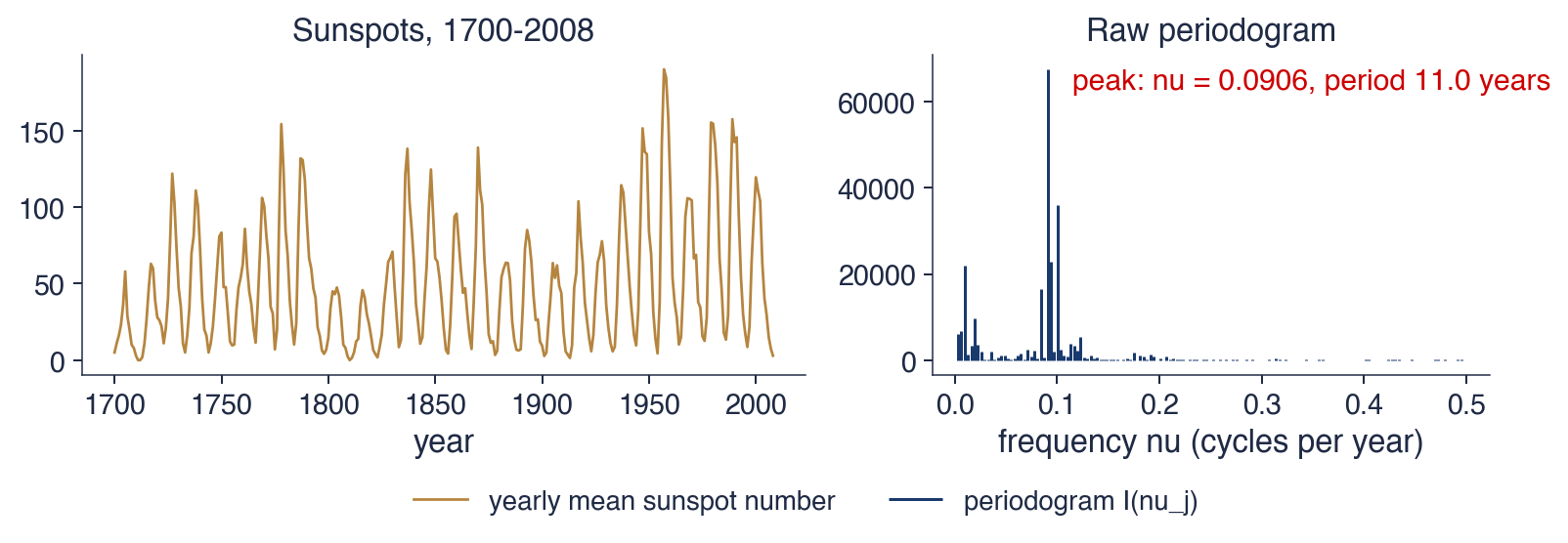
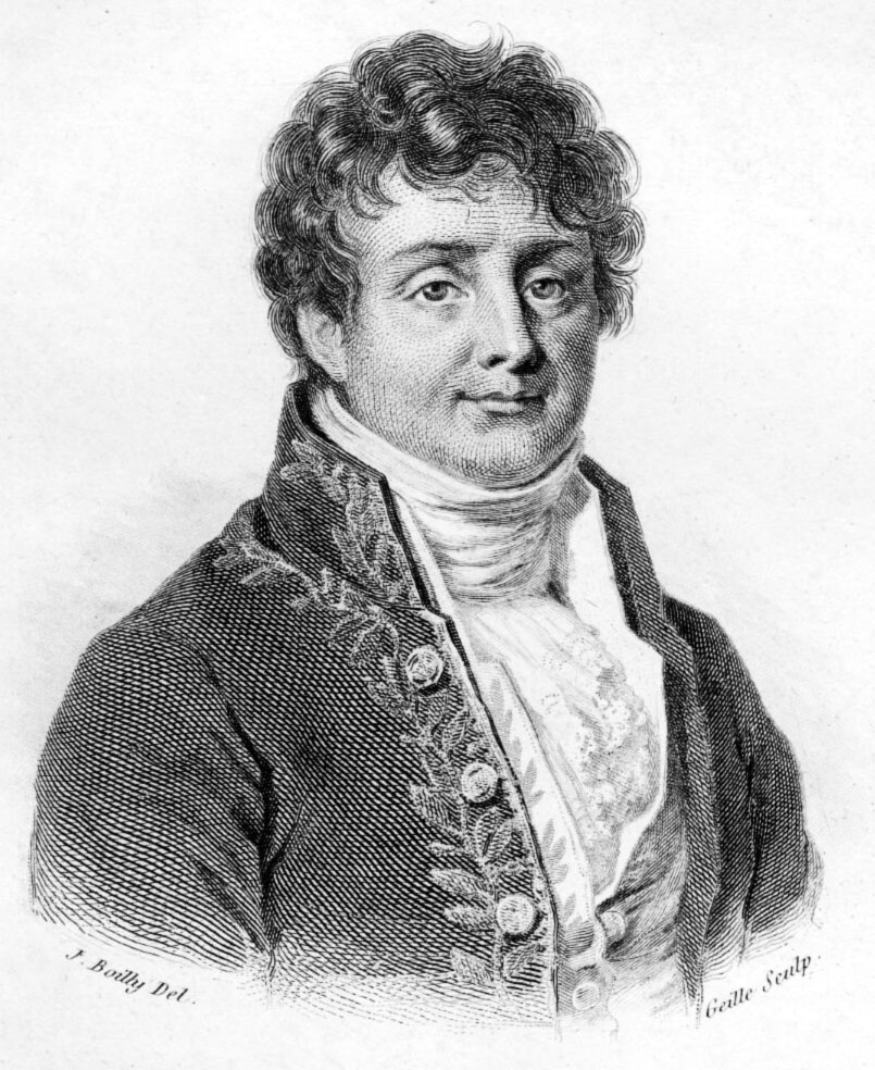
 TSA_ch12_fourier