Bucharest University of Economic Studies IDA Institute Digital Assets Blockchain Research Center AI4EFin Artificial Intelligence for Energy Finance Romanian Academy, Institute for Economic Forecasting MSCA Digital Finance
The question of the chapter starts from two prices that both move like random walks. Each of them, taken alone, cannot be forecast over long horizons. A combination of them, for example their difference or a ratio, may nonetheless be stable over time. If so, the series share a stochastic trend and a long-run equilibrium, and a regression in levels estimates a real relation, not a spurious one.
The route has three parts. The first defines cointegration and tests it with the Engle–Granger method, using the critical values that fit it, then builds the error correction model. The second moves to systems: the VECM, the Granger representation theorem, the Johansen tests, the interpretation of the coefficients and forecasting. The third applies the tools: purchasing power parity, interest rates, three Central European currencies and pairs trading on the Bucharest Stock Exchange. The chapter builds on Chapter 3, for unit roots and spurious regression, and on Chapter 6, for VAR models.
In brief
Question: two prices both wander like random walks; can a combination of them be stable, and how do we model it?
if yes, the series share a common stochastic trend and a long-run equilibrium: regressions in levels are meaningful, not spurious
Route of the chapter
the idea of cointegration; the Engle–Granger two-step method with the right critical values; error correction models
the VECM and the Granger representation theorem; the Johansen tests; estimating and reading \(\beta\) and \(\alpha\); forecasting
applications: purchasing power parity, interest rates, three Central European currencies, pairs trading on the Bucharest Stock Exchange
We build on Chapter 3 (unit roots, spurious regression) and Chapter 6 (VAR models)
The first outcomes concern the concept and its single-equation test. The reader should be able to define cointegration and explain it as a common stochastic trend, to apply the Engle–Granger and Phillips–Ouliaris tests, and to compare the statistics with the critical values of cointegration tests, not with the Dickey–Fuller ones. The reader should then be able to estimate an error correction model and translate the speed of adjustment into a half-life.
The next outcomes concern systems: writing a VAR as a VECM, stating the Granger representation theorem and choosing the cointegrating rank with the Johansen tests, followed by the interpretation of the cointegrating vectors and the adjustment coefficients. The last outcomes concern use: when a VECM forecasts better than a VAR in differences, and how to evaluate an application, from parity conditions to pairs trading, out of sample and after costs.
In brief
Define cointegration and explain it as a common stochastic trend
Run the Engle–Granger and Phillips–Ouliaris tests and compare them with the right (not the Dickey–Fuller) critical values
Estimate an error correction model and interpret the speed of adjustment and the half-life
Write a VAR as a VECM, state the Granger representation theorem and choose the cointegration rank with the Johansen tests
Interpret cointegrating vectors and adjustment coefficients, and decide when a VECM forecasts better than a VAR in differences
Judge an application (parity conditions, pairs trading) out of sample and net of costs
The course textbook is Huang and Petukhina (2022), whose Chapter 9 covers non-stationarity and cointegration. The theory is treated at length in Hamilton (1994), Chapters 19–20, and in Lütkepohl (2005), Chapters 6–8. The maximum-likelihood approach developed by Søren Johansen and Katarina Juselius is set out in Johansen (1995) and, with an emphasis on applications, in Juselius (2006).
The reference papers are Engle and Granger (1987), which defined cointegration, Johansen (1988) and Johansen (1991), which gave the tests for systems, and Granger's Nobel lecture, Granger (2004). The computations are done in Python: coint, coint_johansen, VECM and VAR from statsmodels, and phillips_ouliaris from arch. The chapter's Quantlets reproduce every chart and table, and the lecture notebook runs in Google Colab.
The relationship between co-integration and error correction models, first suggested in Granger (1981), is here extended and used to develop estimation procedures, tests, and empirical examples. If each element of a vector of time series x first achieves stationarity after differencing, but a linear combination a'x is already stationary, the time series x are said to be co-integrated with co-integrating vector a.
Chapter 3 established two facts that seem to close the discussion of series with a stochastic trend. Many economic and financial series are integrated of order 1, \(I(1)\): they become stationary only after one difference. And the regression of one \(I(1)\) series on another, unrelated \(I(1)\) series often produces a spurious result, with large \(t\)-statistics and a large \(R^2\). The cautious conclusion would be to always work in differences. This chapter shows why that conclusion is too hasty.
There is an important case in which two or more \(I(1)\) series are tied together in the long run: some linear combination of them is stationary. The series can drift apart for a while, but the distance between them keeps returning towards an equilibrium level. This case is called cointegration. Granger (1981) formulated the idea, and Engle and Granger (1987) gave the definition, the two-step estimation method and the link to error correction models. Differencing the data would erase exactly this information about the long run.
The chapter builds three tools: the residual-based Engle–Granger test, the single-equation error correction model, and the vector error correction model (VECM), with the Johansen tests for the number of equilibrium relations. It applies them to US Treasury yields, to US consumption and income, to purchasing power parity for the leu, to ROBOR and Euribor, to three Central European currencies and to a pairs-trading strategy on the Bucharest Stock Exchange. The results are mixed, and learning to read a negative result is one of the lessons of the chapter.
Four pairs of trending series: US Treasury yields at 3 months and 10 years (monthly, since 1960), US real GDP and consumption (quarterly, 1959–2009), adjusted share prices of Banca Transilvania and BRD (daily, since 2014) and the EUR/RON and EUR/HUF exchange rates (end of month, since July 2005).
What you will be able to do
Define cointegration and explain it as a stochastic trend shared by several series.
Test for cointegration with the Engle–Granger and Phillips–Ouliaris tests, using the right critical values.
Estimate an error correction model and interpret the speed of adjustment and the half-life.
Derive the VECM form of a VAR and choose the cointegrating rank with the Johansen tests.
Interpret the cointegrating vectors, the adjustment coefficients and the impulse responses of a VECM.
Evaluate the forecasts of a VECM and a pairs-trading strategy out of sample and after costs.
Chapter plan
The idea of cointegrationSpurious regression, the drunk and her dog, the definition and common stochastic trends.
SummaryKey ideas, formulas and self-assessment questions.
The idea of cointegration
The section starts from the problem of spurious regression and shows the case in which a regression between \(I(1)\) series makes sense. The intuition comes from a well-known story, a drunk walking her dog, checked afterwards by simulation. Then come the formal definition of cointegration, its representation through common stochastic trends, the examples from economic theory and the first tests on four pairs of real series.
Granger and Newbold (1974) showed, by simulation, that regressing one random walk on another, independent random walk mostly gives a large \(t\)-statistic, a large \(R^2\) and a Durbin–Watson statistic close to 0. The result is a spurious regression, discussed in Chapter 3. The cause is the regression error: whatever the slope \(b\), the combination \(y_t - a - bx_t\) still contains the stochastic trend of \(y_t\) and that of \(x_t\), so it is itself \(I(1)\). Nothing ties the two series together, and the usual tests, which assume stationary errors, are no longer valid.
The exception is the case in which, for one particular value of \(b\), the combination \(u_t = y_t - a - bx_t\) is stationary. The stochastic trends of the two series then cancel exactly in this combination, and the series are called cointegrated (Granger, 1981; Engle and Granger, 1987). The regression in levels is no longer spurious: it estimates a real long-run relation. The two series can drift apart for a while, but \(u_t\), being stationary, returns towards its mean and brings them back towards each other. In this sense, \(u_t = 0\) describes an equilibrium.
The rest of the chapter answers three questions about this case: how to recognise it in the data, how to test formally whether a combination is stationary, and how to build a model that uses the information in the equilibrium.
In brief
Chapter 3: regressing one \(I(1)\) series on another, unrelated\(I(1)\) series gives large \(t\), high \(R^2\) and a Durbin–Watson statistic near 0 Granger and Newbold (1974)
the error \(y_t - a - b x_t\) is itself \(I(1)\) for every \(b\): nothing ties the two series together
The exception: for one value of \(b\), the combination \(u_t = y_t - a - b x_t\) is stationary
Murray (1994) gave an illustration that has become a classic. A drunk leaves the pub and wanders aimlessly: her position \(x_t\) is a random walk, each step being unpredictable. Her dog wanders too, so its position \(y_t\) is also a random walk. If the two were independent passers-by, the distance between them would be the difference of two random walks, hence again a random walk, and its standard deviation would grow without bound, in proportion to \(\sqrt{t}\).
The drunk and the dog are not independent, however. When they drift apart, the dog hears her call and runs back, and she hears the dog and turns towards it. Each closes part of the distance at every step: \(\Delta x_t = c\,(y_{t-1} - x_{t-1}) + u_t\) and \(\Delta y_t = d\,(x_{t-1} - y_{t-1}) + w_t\), where \(c, d > 0\) are the fractions of the distance closed at each step and \(u_t\) and \(w_t\) are independent shocks. The terms in \(c\) and \(d\) are error correction terms.
The result combines two properties that seem contradictory. Each path remains unpredictable, because the shocks accumulate, but the distance \(y_t - x_t\) stays bounded, because it is corrected at every step. This is, in a single picture, the idea of the chapter: cointegration and error correction are two sides of the same phenomenon.
Murray (1994): a drunk leaves the pub and wanders: her path \(x_t\) is a random walk
her dog also wanders: \(y_t\) is a random walk too
the distance between two independent walkers grows without limit, like \(\sqrt{t}\)
But the dog hears her call and runs back; she hears the dog and turns towards it
each corrects part of the gap: \(\Delta x_t = c\,(y_{t-1} - x_{t-1}) + u_t\), \(\Delta y_t = d\,(x_{t-1} - y_{t-1}) + w_t\); \(c, d > 0\): the shares of the gap closed per step; \(u_t\), \(w_t\): independent shocks
both paths remain unpredictable, but the distance \(y_t - x_t\) stays bounded: cointegration with error correction
Question for the room Set c = d = 0: neither the drunk nor the dog corrects the distance any more. What p-value does ADF give for the distance y − x?
Answer
0.261: the unit root is no longer rejected. Without correction, y − x is the difference of two independent random walks, hence a random walk itself; the standard deviation of the distance rises from 1.86 to 7.07. With c = 0.15 and d = 0.25, ρ = 0.6 and p < 0.001: error correction, not the common starting point, keeps the distance bounded.
The simulation runs the two equations for \(T = 400\) steps, with Gaussian shocks and \(c = 0.15\) and \(d = 0.25\): at each step the drunk closes 15% of the distance and the dog 25%. For comparison, a stray dog \(z_t\) also appears, an independent random walk with the same shock variance.
The left panel shows the three paths. The drunk (\(x_t\)) and her dog (\(y_t\)) wander together: their common path rises and falls without any predictable tendency, but the two lines stay almost on top of each other. The stray dog heads off in another direction and ends, after 400 steps, about 50 units below the other two. The right panel shows the distances: \(y_t - x_t\) oscillates tightly around zero, while \(z_t - x_t\) drifts far away, down to about \(-50\).
In brief
\(T = 400\), Gaussian shocks; \(c = 0.15\), \(d = 0.25\); a stray dog \(z_t\) is an independent random walk with the same shocks' variance
Unit root tests confirm what the chart shows. The augmented Dickey–Fuller (ADF) test applied to the drunk's path gives a p-value of 0.21, so the unit root is not rejected, as expected for a random walk. The distance to her own dog, however, is an AR(1) process: subtracting the two equations, \(y_t - x_t = (1 - c - d)(y_{t-1} - x_{t-1}) + (w_t - u_t)\), with coefficient \(\rho = 1 - 0.15 - 0.25 = 0.6\). The ADF test on this distance gives a p-value below 0.001, and its standard deviation is 1.9. The distance to the stray dog has an ADF p-value of 0.81 and a standard deviation of 14.1, so it behaves like a random walk.
The coefficient \(\rho = 0.6\) also tells how fast a distance closes. After \(h\) steps without new shocks a fraction \(0.6^h\) of it remains, so half of it has gone after \(h = \ln 0.5/\ln 0.6 = 1.4\) steps. This quantity is the half-life, which returns in Section 3 for the estimated models.
The practical consequence matters. Neither the drunk's path nor the dog's can be forecast over long horizons, but knowing where the drunk is tells us where to look for the dog. Cointegration does not make the series predictable; it makes the relation between them predictable.
In brief
Each path is \(I(1)\): ADF on \(x_t\) gives p = 0.21
the distance \(y_t - x_t\) is an AR(1) with \(\rho = 1 - c - d = 0.6\): ADF p \(<\) 0.001, standard deviation 1.9
the distance to the stray dog wanders: ADF p = 0.81, standard deviation 14.1
Half of a gap disappears in \(\ln 0.5/\ln 0.6 = 1.4\) steps: the half-life (Section 3)
knowing where the drunk is tells us where to look for the dog, even though neither path can be forecast
The definition of Engle and Granger (1987) applies to a vector of \(n\) series, \(\mathbf y_t = (y_{1t}, \dots, y_{nt})^\top\). Its components are cointegrated of order (1,1), written \(\mathbf y_t \sim CI(1,1)\), if two conditions hold. First, each component is \(I(1)\), that is, it becomes stationary after one difference, as in Chapter 3. Second, there is a vector \(\beta \neq 0\) for which the linear combination \(\beta^\top\mathbf y_t\) is \(I(0)\), that is, stationary. The first 1 in the notation gives the order of integration of the series, the second by how much this order falls in the combination.
The vector \(\beta\) is called the cointegrating vector, and \(u_t = \beta^\top\mathbf y_t - \mu\), where \(\mu\) is the mean of the combination, is called the equilibrium error. The vector is not unique: if \(\beta^\top\mathbf y_t\) is stationary, so is \(2\beta^\top\mathbf y_t\). One coefficient is therefore normalised to 1; with two variables one usually writes \(\beta = (1, -b)^\top\), which corresponds to the relation \(y_t = a + bx_t + u_t\).
With \(n\) variables there can be several linearly independent cointegrating vectors, but at most \(n - 1\); their number \(r\) is called the cointegrating rank. Cointegration is a property of the levels: if all series are differenced before modelling, the combination \(\beta^\top\mathbf y_t\) disappears from the data and, with it, the information about the equilibrium.
In brief
DefinitionEngle and Granger (1987): the components of \(\mathbf y_t = (y_{1t}, \dots, y_{nt})^\top\) are cointegrated of order (1,1), \(\mathbf y_t \sim CI(1,1)\), if
every component is \(I(1)\) (Chapter 3: stationary after one difference), and
some linear combination \(\beta^\top \mathbf y_t\), with \(\beta \neq 0\), is \(I(0)\): stationary
\(\beta\) is the cointegrating vector; \(u_t = \beta^\top \mathbf y_t - \mu\) is the equilibrium error (\(\mu\): its mean; \(\top\): transpose)
\(\beta\) is unique only up to scale: \(2\beta\) works as well; we normalise one coefficient to 1, e.g. \(\beta = (1, -b)^\top\)
with \(n\) variables there can be up to \(r = n - 1\) independent cointegrating vectors; \(r\) is the cointegration rank
Cointegration is a property of the levels: differencing the data destroys the information in \(\beta^\top \mathbf y_t\)
A simple example shows the mechanism. Let \(x_t = x_{t-1} + \varepsilon_t\) be a random walk and \(y_t = bx_t + u_t\), with \(u_t\) stationary. Both series contain the same stochastic trend, the sum of past shocks \(\sum_{s \le t}\varepsilon_s\):\(x_t\) contains it with weight 1, \(y_t\) with weight \(b\). The combination \(y_t - bx_t = u_t\) removes it completely and stays stationary. Cointegration therefore means that the series are driven by shared trends, not each by its own.
Stock and Watson (1988) turned this observation into a general common trends representation: \(n\) variables with \(r\) cointegrating vectors are driven by \(n - r\) common stochastic trends. The two extremes are instructive. With \(r = 0\) there are \(n\) separate trends and no cointegration. With \(r = n - 1\) there is a single trend, shared by all the series. The Treasury yields at 1, 5 and 10 years, with \(r = 2\), have a single common trend, the general level of interest rates, as Section 5 shows.
The worked example uses three series: \(x_t\) a random walk, \(y_t = 2x_t + u_t\) and \(z_t = -x_t + v_t\), with \(u_t\) and \(v_t\) stationary. All three are driven by the same trend, so \(n = 3\),\(n - r = 1\) and \(r = 2\). In the order \((x_t, y_t, z_t)\), two cointegrating vectors are \(\beta_1 = (-2, 1, 0)^\top\), because \(y_t - 2x_t = u_t\), and \(\beta_2 = (0, 1, 2)^\top\), because \(y_t + 2z_t = 2x_t + u_t - 2x_t + 2v_t = u_t + 2v_t\). Any linear combination of the two vectors is again a cointegrating vector; the rank says how many independent directions exist.
In brief
Write \(x_t = x_{t-1} + \varepsilon_t\) (a random walk) and \(y_t = b\,x_t + u_t\), with \(u_t\) stationary
both series contain the same stochastic trend \(\sum_{s \le t} \varepsilon_s\); \(y_t - b x_t = u_t\) removes it
Common trends representation Stock and Watson (1988): \(n\) variables with \(r\) cointegrating vectors are driven by \(n - r\) common stochastic trends
\(r = 0\): \(n\) separate trends, no cointegration; \(r = n - 1\): one trend shared by all
example: three yields (1, 5 and 10 years) with \(r = 2\) share one trend, the level of interest rates (Section 5)
Worked example: \(x_t\) a random walk, \(y_t = 2x_t + u_t\), \(z_t = -x_t + v_t\) (\(u_t\), \(v_t\) stationary)
\(n = 3\), one common trend, so \(r = 2\): in the order \((x_t, y_t, z_t)\), e.g. \(\beta_1 = (-2, 1, 0)^\top\) and \(\beta_2 = (0, 1, 2)^\top\) (since \(y_t - 2x_t = u_t\) and \(y_t + 2z_t = u_t + 2v_t\))
Many economic theories state that some combination of non-stationary variables must be stable. Purchasing power parity (PPP) writes the log exchange rate as \(s_t = p_t - p_t^* + q_t\), where \(s_t\) is the log exchange rate (lei per euro), \(p_t\) and \(p_t^*\) are the logs of the domestic and foreign price levels, and \(q_t\) is the real exchange rate. The theory requires \(q_t\) to be stationary, which means cointegration of \(s_t\),\(p_t\) and \(p_t^*\);Section 8 tests this requirement for the leu.
The term structure of interest rates gives the second example. Under the expectations hypothesis, a long-term yield is the average of expected short-term yields plus a premium; the difference (the spread) between the long and the short yield is then stationary (Campbell and Shiller, 1987). The third example is the "great ratios": if consumption follows permanent income, the ratio of consumption to income, \(c_t - y_t\) in logs, is stable.
The last examples come from financial markets. Arbitrage keeps small the difference between the spot price and the futures price of the same asset, or between an index and a fund that tracks it. The shares of similar firms are exposed to the same sector shocks and may share a trend; this is the basis of the pairs-trading strategy in Section 9. In every case, theory proposes a relation and the data must confirm it.
In brief
Purchasing power parity: \(s_t = p_t - p^*_t + q_t\), with the real exchange rate \(q_t\) stationary (Section 8)
\(s_t\): log exchange rate (lei per euro); \(p_t\), \(p^*_t\): log price levels at home and abroad
Term structure of interest rates: by the expectations hypothesis, the spread between a long and a short yield is stationary Campbell and Shiller (1987)
Consumption and income: the “great ratio” \(c_t - y_t\) (logs) is stable if consumption follows permanent income
Spot and futures prices, an index and a fund that tracks it: arbitrage keeps the gap small
Shares of similar firms: the same sector shocks; the basis of pairs trading (Section 9)
Question for the room Set a = 1 (c = −1). What is the second cointegrating vector?
Answer
β₂ = (0, 1, 1)ᵀ: yt + zt = ut + vt, with no trend. The vector depends on the coefficients: in general β₂ = (0, 1, −a/c)ᵀ, hence (0, 1, 2)ᵀ for a = 2 and c = −1. The rank stays 2, because three series still share one common trend.
Question for the room Drop the first 50% of each sample. Does Engle–Granger still reject “no cointegration” at 5% for US consumption and GDP?
Answer
No: τ = −1.95, p = 0.553 on the last 102 quarters, against τ = −3.54, p = 0.029 on 203. With half the data and deviations that last years, the test has little power; a large p means that the relation is not separated from noise in this sample, not that it does not exist. For the banks the test stays below 5% (p = 0.044).
The chart shows four pairs of series used throughout the chapter. The first panel contains the US Treasury yields at 3 months and 10 years, in percent per year, monthly since 1960, from the FRED database (Federal Reserve Economic Data). The second contains US real GDP and consumption, quarterly from 1959 to 2009, as 100 × the natural log, set to 0 in the first quarter of 1959; on this scale a difference of 1 unit means approximately 1%.
The third panel shows the adjusted share prices of Banca Transilvania (TLV) and BRD since 2014, and the fourth the EUR/RON and EUR/HUF reference rates published by the National Bank of Romania (BNR), at the end of the month, since July 2005, both as 100 × log, set to 0 at the start. In every panel the two series seem to move together. The chart alone cannot say, however, whether this impression reflects a common trend or just two separate trends that happened to point the same way in the sample.
In brief
US Treasury yields (FRED, monthly, since 1960); US real GDP and consumption (statsmodels macrodata, 1959–2009)
Banca Transilvania and BRD (adjusted daily prices); EUR/RON and EUR/HUF (BNR reference rates, month-end)
Each of the eight series is \(I(1)\) according to the tests of Chapter 3. The question is whether the two series of each pair move together in the long run, and the answer comes from the Engle–Granger test of Section 2. Its statistic, \(\tau\), is compared with a 5% critical value of about \(-3.34\); a more negative value rejects the null hypothesis of no cointegration.
For the 10-year yield on the 3-month yield, \(\tau = -3.35\) with p-value 0.048, a borderline result. For consumption and income, \(\tau = -3.54\) with p-value 0.029, and for the two banks \(\tau = -4.33\) with p-value 0.002: these are cointegrated in the sample since 2014. For EUR/RON and EUR/HUF, \(\tau = -2.47\) with p-value 0.294: the test does not reject the null of no cointegration, so the data give no evidence of a common trend of the two exchange rates.
The last pair is the most instructive. The two exchange rates have risen by similar amounts since 2005, and the regression in levels has \(R^2 = 0.79\). A common direction in the sample is not a common stochastic trend, however: the paths of the two series have parted several times, for example after 2020, and no force brings them back together.
In brief
Each series is \(I(1)\) (Chapter 3); the question is whether the two series of a pair move together in the long run
Engle–Granger test (Section 2), 5% critical value about \(-3.34\)
Yields: \(\tau = -3.35\), p = 0.048: borderline; consumption and income: \(\tau = -3.54\), p = 0.029
The two banks: \(\tau = -4.33\), p = 0.002: cointegrated in this sample
EUR/RON and EUR/HUF: \(\tau = -2.47\), p = 0.294: no evidence of cointegration
although they rose by similar amounts and \(R^2 = 0.79\) in levels: a common direction is not a common trend
First question: two \(I(1)\) series have a correlation of 0.95 in levels; are they cointegrated? The correlation does not answer the question. Unrelated random walks often have large correlations in levels; this is the very phenomenon of spurious regression in Chapter 3. Only a test applied to the equilibrium error, that is, the question whether a combination of the series is stationary, can decide.
Second question: two cointegrated series have a correlation of 0.2 between their daily changes; is this a contradiction? No. Cointegration concerns the long run: the series do not drift apart indefinitely. In the short run their changes can be almost uncorrelated, and the correction of the distance can work slowly, over many days. The correlation of the changes and the cointegration of the levels are different properties.
In brief
Question: two \(I(1)\) series have a correlation of 0.95 in levels. Are they cointegrated?
Answer: we cannot tell: unrelated random walks often have high correlations (Chapter 3); only a test on the equilibrium error decides
Question: two cointegrated series have a correlation of 0.2 between their daily changes. Is this a contradiction?
Answer: no: cointegration is about the long run; in the short run the changes can be almost unrelated
\(I(1)\) series are cointegrated if a linear combination \(\beta^\top\mathbf y_t\) is stationary; the combination describes a long-run equilibrium, and deviations from it are corrected. An equivalent statement is that the series share stochastic trends: \(n\) variables with \(r\) cointegrating vectors are driven by \(n - r\) trends. Economic theory suggests cointegration in many places, from parity conditions to spreads and "great ratios", but the data must confirm it through a test.
In brief
\(I(1)\) series are cointegrated if a combination \(\beta^\top \mathbf y_t\) is stationary: a long-run equilibrium
Equivalently, they share common stochastic trends: \(n\) variables, \(r\) vectors, \(n - r\) trends
Theory suggests cointegration (parity conditions, spreads, great ratios), but the data must confirm it
Section summary
Cointegration is the exception to the rule of spurious regression: series that, taken alone, are unpredictable random walks can be tied by a stationary combination. The simulation of the drunk and her dog shows that a distance corrected at every step stays bounded although both paths wander. On real data, the Engle–Granger test finds cointegration for consumption and income and for two Romanian banks, a borderline result for two US yields and no evidence for EUR/RON and EUR/HUF. The next section explains the test and its critical values.
The Engle–Granger two-step method
The method of Engle and Granger (1987) is the simplest way to test two series for cointegration: a regression in levels, followed by a unit root test on the residuals. The simplicity hides a trap: the critical values are no longer the Dickey–Fuller ones. The section explains why, obtains them by simulation, presents the alternative Phillips–Ouliaris test, applies both tests to real data and closes with the limits of the method.
Step 1 estimates the long-run relation by ordinary least squares (OLS) in levels, \(y_t = a + bx_t + u_t\), and keeps the residuals \(\hat u_t = y_t - \hat a - \hat bx_t\). If the series are cointegrated, the estimator \(\hat b\) has an unusual property: it is super-consistent, meaning that its error shrinks like \(1/T\), faster than the usual rate \(1/\sqrt{T}\). The intuition is that any wrong value of \(b\) leaves a stochastic trend in the residuals, whose variance then grows with the sample; OLS, which minimises this variance, finds the right value very quickly.
Step 2 applies an ADF test, as in Chapter 3, to the step-1 residuals, without a constant, because OLS residuals already have mean zero:
Here \(\delta_j\) are the coefficients of the \(k\) lagged differences, which absorb the autocorrelation of \(\hat u_t\), and \(e_t\) is white noise. The null hypothesis \(\gamma = 0\) states that the residuals have a unit root, so there is no cointegration; the alternative \(\gamma < 0\) states that the residuals revert towards zero. The test statistic is \(\tau = \hat\gamma/\mathrm{SE}(\hat\gamma)\), where SE is the standard error, and the null is rejected when \(\tau\) is below the critical value.
The test has a precondition: each series must be \(I(1)\). An \(I(0)\) series and an \(I(1)\) series cannot be cointegrated, because any combination with a non-zero coefficient on the \(I(1)\) series remains \(I(1)\). That is why every cointegration analysis starts with unit root tests on each series.
In brief
Step 1: estimate the long-run relation by OLS (ordinary least squares) in levels: \(y_t = a + b\,x_t + u_t\)
keep the residuals \(\hat u_t = y_t - \hat a - \hat b x_t\)
if the series are cointegrated, \(\hat b\) is super-consistent: its error shrinks like \(1/T\), faster than the usual \(1/\sqrt{T}\)
Step 2: an ADF test (Chapter 3) on the residuals, without a constant: \(\Delta\hat u_t = \gamma\,\hat u_{t-1} + \sum_{j=1}^{k}\delta_j\Delta\hat u_{t-j} + e_t\)
\(H_0\): \(\gamma = 0\), the residuals have a unit root: no cointegration; \(H_1\): \(\gamma < 0\): cointegration
\(\delta_j\): coefficients of the \(k\) lagged differences, which absorb the autocorrelation of \(\hat u_t\); \(e_t\): white noise
statistic \(\tau = \hat\gamma/\mathrm{SE}(\hat\gamma)\), SE: standard error; reject \(H_0\) when \(\tau\) is below the critical value
Pretest: each series must be \(I(1)\); cointegration between an \(I(0)\) and an \(I(1)\) series is impossible
The step-1 residuals are not an observed series but the result of an optimisation. OLS chooses \(\hat b\) so that the variance of the residuals is as small as possible, that is, so that \(\hat u_t\) looks as "calm" as possible. Even when the series are not cointegrated, \(\hat u_t\) therefore looks more stationary than the true error \(u_t\). Under the null, the statistic \(\tau\) is pushed towards negative values, and its distribution lies to the left of the Dickey–Fuller distribution.
The right critical values depend on the number of variables \(n\) in the regression and on the deterministic terms in step 1 (a constant, or a constant and a trend). Engle and Granger (1987) obtained them by simulation; MacKinnon (1994) and MacKinnon (2010) then gave accurate approximations, for any sample size, which the coint function of statsmodels uses.
There is one case in which the Dickey–Fuller table is the right one: when the cointegrating vector is known from theory. If theory says that the spread between two rates is stationary, that is \(\beta = (1, -1)^\top\), the spread is computed directly, without any estimation, and the ordinary ADF test, with its own table, is applied to this observed series.
In brief
OLS chooses \(\hat b\) to make the residual variance as small as possible
so \(\hat u_t\) looks more stationary than the true \(u_t\), even when there is no cointegration
under \(H_0\) the statistic \(\tau\) is shifted to the left of the Dickey–Fuller distribution
The critical values depend on the number of variables \(n\) and on the deterministic terms of step 1
Question for the room Switch to T = 50. What is the 5% critical value for n = 2, with a constant?
Answer
−3.46, against −3.34 asymptotically and −3.37 at T = 200. In small samples the distribution of the statistic is shifted further to the left, so the critical values are more negative; the Dickey–Fuller table (−2.92 at T = 50) would be even further from the right one.
Question for the room Switch to T = 50. With the 5% Dickey–Fuller critical value, what share of the samples with 2 variables would reject a true null?
Answer
14.2%, about as at T = 200 (14.5%), and 30.0% with 3 variables. The distortion comes from OLS choosing b̂ to make the residuals as small as possible, not from the sample length; at T = 50 the right critical value for 2 variables is −3.46 (simulated quantile −3.41), against −2.92 in the Dickey–Fuller table.
The simulation builds the distribution of the statistic \(\tau\) under the null. It generates 10,000 samples of \(T = 200\) observations, each made of independent Gaussian random walks, hence without cointegration. For each sample, step 1 is run with a constant and step 2 without lags, and \(\tau\) is recorded. The smoothed histograms of the 10,000 values give the distributions in the chart.
The chart shows four curves. The dashed line is the standard Normal distribution, the usual distribution of a \(t\)-statistic. The blue curve is the Dickey–Fuller distribution for one series with a constant, already far to the left of zero. The red and green curves are the Engle–Granger distributions for 2 and 3 variables, shifted even further left. The dotted vertical lines mark the 5% quantiles of the three non-standard distributions: the more variables, the more negative the critical value.
In brief
10 000 samples of \(T = 200\) independent Gaussian random walks; step 1 with a constant, step 2 without lags
The 5% quantiles from the simulation are \(-2.86\) for a single series (the Dickey–Fuller case), \(-3.33\) for 2 variables and \(-3.75\) for 3 variables. The MacKinnon values for \(T = 200\) are \(-2.88\),\(-3.37\) and \(-3.78\), so the simulation reproduces them up to simulation error.
The difference between the tables has large consequences. If the residual statistic were compared with the Dickey–Fuller value \(-2.88\), a true null would be rejected in 14.5% of the samples with 2 variables and in 30.3% of those with 3 variables, instead of 5%. In other words, cointegration between independent random walks would be "found" three to six times more often than the level of the test promises.
The reason why the critical values grow in absolute value with the number of variables is the one from the previous frame: each additional variable gives OLS one more coefficient with which to reduce the variance of the residuals, so the residuals look even more stationary.
The table gives the asymptotic critical values, for \(T \to \infty\), from MacKinnon (2010), at the 1%, 5% and 10% levels, for 1–4 variables and for two specifications of step 1. The first row, with a single variable, is the ordinary Dickey–Fuller test and serves as a benchmark: the 5% value with a constant is \(-2.86\). For 2 variables it becomes \(-3.34\), for 3 variables \(-3.74\), and for 4 variables \(-4.10\).
The row is chosen by the total number of variables in the regression, including \(y_t\); a regression of \(y_t\) on \(x_t\) uses the row \(n = 2\). In finite samples the critical values are slightly more negative than the asymptotic ones, for example \(-3.37\) instead of \(-3.34\) for 2 variables and \(T = 200\); software computes the value appropriate for \(T\).
The right-hand columns are used when step 1 also includes a deterministic trend. This specification fits when the series have drifts (average growth) that the cointegrating relation does not cancel; the critical values are then even more negative, for example \(-3.78\) at 5% for 2 variables.
In brief
Variables \(n\)
constant
constant and trend
1%
5%
10%
1%
5%
10%
1 (Dickey–Fuller)
\(-3.43\)
\(-2.86\)
\(-2.57\)
\(-3.96\)
\(-3.41\)
\(-3.13\)
2
\(-3.90\)
\(-3.34\)
\(-3.04\)
\(-4.33\)
\(-3.78\)
\(-3.50\)
3
\(-4.29\)
\(-3.74\)
\(-3.45\)
\(-4.66\)
\(-4.12\)
\(-3.84\)
4
\(-4.64\)
\(-4.10\)
\(-3.81\)
\(-4.97\)
\(-4.43\)
\(-4.15\)
Asymptotic values (\(T \to \infty\)) of MacKinnon (2010); for finite \(T\) the values are slightly more negative
Read the row of the total number of variables in the regression, \(y_t\) included
Constant and trend in step 1: when the series have drifts that the relation does not cancel
Phillips and Ouliaris (1990) proposed a test with the same step 1 and the same null hypothesis, no cointegration. The difference is in step 2: the Dickey–Fuller regression on the residuals is estimated without lagged differences, and the autocorrelation of the residuals is handled by correcting the \(t\)-statistic with the long-run variance of the residuals, as in the Phillips–Perron test of Chapter 3. The test has two versions: \(Z_t\), the corrected \(t\)-ratio, and \(Z_\alpha\), the corrected statistic \(T\hat\gamma\). The asymptotic critical values of \(Z_t\) are the same as for the Engle–Granger test.
Using both tests has a practical reason. The Engle–Granger test depends on the number of lags \(k\), usually chosen by the Akaike information criterion (AIC), while the Phillips–Ouliaris test depends on the bandwidth used for the long-run variance. The two choices handle the same autocorrelation in different ways. When the tests agree, the verdict is robust; when they disagree, the residual plot and the sample must be examined.
In Python, the Engle–Granger test is coint(y, x) from statsmodels, and the Phillips–Ouliaris test is phillips_ouliaris(y, x, test_type="Zt") from arch.
step 2: a Dickey–Fuller regression without lagged differences; the \(t\)-statistic is corrected with the long-run variance of the residuals (as in the Phillips–Perron test of Chapter 3)
two versions: \(Z_t\) (corrected \(t\)-ratio) and \(Z_\alpha\) (corrected \(T\hat\gamma\)); the critical values of \(Z_t\) are those of Engle–Granger
Reasons for two tests
Engle–Granger depends on the number of lags \(k\) chosen by AIC; Phillips–Ouliaris depends on the bandwidth of the long-run variance
when they agree, the verdict is robust; when they disagree, look at the residual plot and at the sample
In Python: coint(y, x) from statsmodels; phillips_ouliaris(y, x, test_type="Zt") from arch
The data are US real consumption and real GDP, quarterly, from the first quarter of 1959 to the third quarter of 2009, that is, 203 quarters. Both are transformed into \(c_t\) and \(y_t\), 100 × the natural log, so that one unit means approximately 1%. The preliminary ADF tests with trend give p-values of 0.31 for \(c_t\) and 0.39 for \(y_t\), so both series are treated as \(I(1)\).
Step 1 gives \(\hat c_t = -107.6 + 1.075\,y_t\), with \(R^2 = 0.9992\) and a Durbin–Watson (DW) statistic of the residuals of 0.24. The DW statistic is about 2 when the residuals are not autocorrelated and approaches 0 when they are highly persistent. The slope close to 1 suggests a stable share of consumption in income. Neither an \(R^2\) near 1 nor a small DW proves anything, however: the same combination appears in a spurious regression.
Step 2 gives \(\tau = -3.54\), with 0 lags chosen by AIC. The 5% critical value for \(n = 2\) and \(T = 203\) is \(-3.37\). Since \(-3.54 < -3.37\), the hypothesis "no cointegration" is rejected at 5%, with p-value 0.029; the Phillips–Ouliaris test gives \(Z_t = -3.52\), with p-value 0.031. Comparing with the Dickey–Fuller value, \(-2.88\), would have led to the same decision here, but for the wrong reason: with a statistic between \(-3.37\) and \(-2.88\), it would have led to a wrong conclusion.
In brief
Data: \(c_t\), \(y_t\) = 100 \(\times\) log of real consumption and real GDP, quarterly, 1959Q1–2009Q3 (203 quarters)
pretest: ADF with trend, p = 0.31 for \(c_t\) and 0.39 for \(y_t\): both \(I(1)\)
Question for the room End the sample in 1985. Is “no cointegration” rejected at 5%?
Answer
No: τ = −3.00 against the Engle–Granger critical value −3.39 (p = 0.111), on 108 quarters. With the Dickey–Fuller value (−2.89) it would be rejected, wrongly. R² stays above 0.99 and the slope is 1.072, but neither a high R² nor a slope close to 1 proves cointegration.
Worked example
\[\Delta\hat u_t=\gamma\,\hat u_{t-1}+\textstyle\sum_{j=1}^{k}\delta_j\Delta\hat u_{t-j}+e_t,\qquad \tau=\dfrac{\hat\gamma}{\mathrm{SE}(\hat\gamma)}\ \text{against the Engle–Granger critical value}\]
Question for the room Drop the first 30% of each sample. Is there still no evidence of cointegration for TLV on BRD since 2010?
Answer
There is now: τ = −3.98, p = 0.008 (Phillips–Ouliaris p = 0.001), against p = 0.622 on the whole sample since 2010. Without 2010–2014 the relation between the two banks appears; the same pair gives opposite verdicts depending on the start date, which is why choosing the sample after seeing the data is data snooping.
Question for the room Drop the first 50% of each sample. Does the lag-8 autocorrelation of the consumption residuals fall?
Answer
No: it rises from 0.31 to 0.46, and for the yields ρ̂(12) rises from 0.58 to 0.62. In the second half of the samples the deviations from the long-run relation last longer; the persistence of the residuals depends on the period, which is why the test, not the shape of the ACF, decides.
The chart shows the step-1 residuals \(\hat u_t\) for two regressions: consumption on income (left, quarterly) and the 10-year yield on the 3-month yield (centre, monthly). Both oscillate around zero, but in long waves: the consumption residuals stay below zero for most of the 1960s and above zero after 2000, and the yield residuals have cycles of several years, with the largest deviations around 1980.
The right panel compares the sample autocorrelation functions (ACF) of the two residual series with the ACF of a simulated random walk (dashed line). The ACF of the consumption residuals falls quickly and crosses below zero after about 14 lags. The ACF of the yield residuals falls much more slowly. The ACF of the random walk stays close to 1 and falls only to about 0.7 after 24 lags.
In brief
Left and centre: \(\hat u_t\) of consumption on income and of the 10-year on the 3-month Treasury yield; right: their sample ACF and that of a simulated random walk
For consumption, the residual autocorrelation is 0.86 at lag 1 but only 0.31 at lag 8. Deviations from equilibrium, of the order of 1–3%, persist from one quarter to the next but shrink considerably within about two years. For the yields, the autocorrelation is 0.97 at lag 1 and still 0.58 at lag 12: deviations last for years, and the test is borderline (\(\tau = -3.35\), p-value 0.048).
High persistence is the usual situation for equilibrium errors, not an exception. An AR(1) process with \(\rho\) close to 1 is hard to tell apart from a random walk in a finite sample; the power of unit root tests against such alternatives is low, as in Chapter 3. A borderline result for very persistent series must therefore be read with caution in both directions.
The comparison with the random walk also shows the limit of visual inspection. The ACF of a random walk decays much more slowly than that of the residuals, but the difference between slow and very slow decay cannot be settled by eye. The test turns this difference into a decision with a known significance level.
In brief
Consumption: \(\hat\rho(1) = 0.86\) but \(\hat\rho(8) = 0.31\): deviations of 1–3% that shrink markedly within about two years
Yields: \(\hat\rho(1) = 0.97\), \(\hat\rho(12) = 0.58\): very persistent deviations; a borderline test (\(\tau = -3.35\), p = 0.048)
high persistence is the usual situation: the power of the test against \(\rho\) close to 1 is low (Chapter 3)
A random walk decays much more slowly: the ACF alone cannot settle the question; the test can
The table applies both tests to seven regressions. For each, the columns give the data frequency, the number of observations \(T\), the estimated slope \(\hat b\), the Engle–Granger statistic \(\tau\) with the number of lags \(k\) chosen by AIC, its p-value, the Phillips–Ouliaris statistic \(Z_t\) and its p-value. The p-values come from the approximations of MacKinnon (2010) for 2 variables.
The first rows repeat the examples already discussed: US consumption on income (\(\tau = -3.54\), p-value 0.029) and the 10-year yield on the 3-month yield (\(\tau = -3.35\) with 20 lags, p-value 0.048, while \(Z_t = -4.04\), p-value 0.006). Then comes the bank pair in three versions: TLV on BRD since 2014 (p-value 0.002), the reverse regression BRD on TLV since 2014 (p-value 0.004) and TLV on BRD since 2010 (p-value 0.622). The EUR/RON and EUR/HUF exchange rates have a p-value of 0.294.
The last row uses Romanian household consumption and GDP, from Eurostat, in chain-linked volumes, seasonally adjusted, quarterly since 1995, 126 observations. The slope is 1.46, and the two tests give opposite verdicts: p-value 0.363 for Engle–Granger, with 8 lags, and below 0.001 for Phillips–Ouliaris.
In brief
Regression
Freq.
\(T\)
\(\hat b\)
\(\tau\) (k)
p
\(Z_t\)
p
US consumption on income
quarterly
203
1.07
\(-3.54\) (0)
0.029
\(-3.52\)
0.031
US: 10-year on 3-month yield
monthly
801
0.86
\(-3.35\) (20)
0.048
\(-4.04\)
0.006
TLV on BRD (since 2014)
daily
3 176
1.36
\(-4.33\) (3)
0.002
\(-4.14\)
0.005
BRD on TLV (since 2014)
daily
3 176
0.71
\(-4.16\) (3)
0.004
\(-4.02\)
0.007
TLV on BRD (since 2010)
daily
4 187
1.68
\(-1.82\) (3)
0.622
\(-1.83\)
0.619
EUR/RON on EUR/HUF
monthly
255
0.71
\(-2.47\) (0)
0.294
\(-2.43\)
0.309
Romania: consumption on GDP
quarterly
126
1.46
\(-2.32\) (8)
0.363
\(-6.80\)
\(<\) 0.001
\(\tau\): Engle–Granger statistic (\(k\) lags by AIC); p-values of MacKinnon (2010) for 2 variables; \(Z_t\): Phillips–Ouliaris
Banks: adjusted prices from data/market; Romania: household consumption and GDP, Eurostat, chain-linked volumes, seasonally adjusted, since 1995
The first lesson concerns normalisation. The regression of TLV on BRD gives \(\tau = -4.33\), and the regression of BRD on TLV gives \(\tau = -4.16\); the slopes, 1.36 and 0.71, are not exact inverses of each other, since \(1/1.36 = 0.74\). OLS minimises errors in the direction of the left-hand variable, so the result depends on that choice. Here the verdict is the same in both directions, but this is not guaranteed in general.
The second lesson concerns the sample. Since 2010, the same banks have a p-value of 0.622, and the test does not detect cointegration; since 2014, the p-value is 0.002. Choosing the start date after examining the data and seeing which one gives the desired result is a form of data snooping, that is, searching the data until a result appears; a p-value obtained this way no longer has its nominal meaning.
The third lesson concerns disagreement between the tests. For Romania, Engle–Granger with 8 lags does not reject no cointegration, while Phillips–Ouliaris rejects it at any usual level. The slope of 1.46 is far from 1: the share of consumption in GDP rose strongly over the period, and such a relation can be hard to tell apart from an unstable one. Seminar 7 (B2) discusses this case.
In brief
Normalisation: TLV on BRD and BRD on TLV give different \(\tau\) (\(-4.33\) and \(-4.16\)) and slopes that are not exact inverses
Engle–Granger depends on which variable is on the left; here the verdict is the same
The sample: since 2010 the test finds no cointegration for the same banks (p = 0.622); since 2014 it does (p = 0.002)
choosing the start date after looking at the data is a form of data snooping
The two tests disagree for Romania: Engle–Granger p = 0.363 with 8 lags, Phillips–Ouliaris p \(<\) 0.001
the slope 1.46 is far from 1: the consumption share rose strongly; Seminar 7 (B2) discusses this case
The method has four limits. First, it can find at most one cointegrating vector. With two variables this is not a problem, but with \(n \ge 3\) variables there may be several vectors, and a single regression estimates only one combination of them (Sections 4–5). Second, the results depend on the variable placed on the left, as the bank pair showed.
The third limit concerns inference on \(\hat b\). The estimator is super-consistent but biased in small samples, and the \(t\)-statistics reported by OLS in step 1 are not valid, because the errors are autocorrelated and correlated with the changes in \(x_t\). One remedy is the dynamic OLS (DOLS) estimator of Stock and Watson (1993), which adds leads and lags of \(\Delta x_t\) to the regression and gives valid standard errors.
The fourth limit comes from the two-step structure: estimation errors in step 1 carry over into step 2, and the power of the test is low when adjustment to equilibrium is slow. The Johansen method of Section 5 avoids these problems by estimating everything at once, by maximum likelihood, in a system.
In brief
At most one cointegrating vector: with \(n \ge 3\) variables there may be several (Sections 4–5)
Normalisation: the results depend on the variable put on the left
Inference on \(\hat b\): super-consistent, but biased in small samples, and its OLS \(t\)-statistics are not valid
remedy: dynamic OLS (DOLS) Stock and Watson (1993), adding leads and lags of \(\Delta x_t\), gives valid standard errors
Two-step errors: mistakes in step 1 carry over to step 2; the power is low against slow adjustment
the Johansen method (Section 5) estimates everything at once, by maximum likelihood
The question of the paper was how to model \(I(1)\) series tied in the long run without falling into the trap of spurious regression and without removing, by differencing, the information about the long run. Engle and Granger (1987), written at the University of California, San Diego, became one of the most cited papers in econometrics.
The contribution has three parts. The first is the definition of cointegration and the representation theorem of Section 4, which shows that cointegrated series always have an error correction representation and conversely. The second is the two-step estimator and the residual-based tests, with critical values obtained by simulation, that is, the method of this section. The third is the applications to US series: consumption and income, prices and wages, short-term and long-term interest rates.
Robert Engle received the 2003 Nobel Prize in economics jointly with Clive Granger; Engle's share was for the ARCH models of Chapter 5, and Granger's for cointegration.
The method has two steps: OLS in levels, with a super-consistent estimator \(\hat b\), and an ADF test on the residuals (7.1), with the null hypothesis of no cointegration. The critical values are the Engle–Granger values computed by MacKinnon, more negative than the Dickey–Fuller ones and dependent on the number of variables. A verdict is checked with the Phillips–Ouliaris test, with the reverse normalisation and on another sample.
In brief
Step 1: OLS in levels (super-consistent \(\hat b\)); step 2: ADF on the residuals, \(H_0\): no cointegration
Critical values of Engle–Granger (MacKinnon), more negative than Dickey–Fuller and dependent on \(n\)
Check with Phillips–Ouliaris, with the reverse normalisation and with another sample
Section summary
The Engle–Granger test is simple, but it needs the right table: because OLS makes the residuals look stationary, the Dickey–Fuller critical values would find cointegration between independent series three to six times more often than they promise. On real data, US consumption and income and the TLV–BRD pair since 2014 are cointegrated according to both tests; the same pair since 2010, the EUR/RON and EUR/HUF rates and, according to Engle–Granger, Romanian consumption and GDP give no evidence of cointegration. Dependence on normalisation, on the sample and on the lag choice are the limits that motivate methods for systems.
Error correction models
If two series are cointegrated, yesterday's equilibrium error contains information about today's changes. The error correction model (ECM) puts this information into a regression in differences. The section defines the model, translates the adjustment coefficient into a half-life, estimates ECMs for US consumption and for the 10-year yield and presents the DHSY consumption function, the first famous application of this form.
Let \(u_{t-1} = y_{t-1} - a - bx_{t-1}\) be the equilibrium error of the previous period. The error correction model explains the change in \(y_t\) by the current and past changes of the variables and by this error:
Here \(c\) is the intercept, \(\phi_j\) and \(\delta_j\) are the short-run coefficients of the lagged differences, and \(\varepsilon_t\) is white noise. If the series are cointegrated, all the terms of the equation are stationary: the differences because the series are \(I(1)\), and \(u_{t-1}\) by the definition of cointegration. That is why OLS and the usual \(t\)-tests are valid, and \(\hat u_{t-1}\) from step 1 of the Engle–Granger method can be used in place of \(u_{t-1}\), thanks to the super-consistency of \(\hat b\).
The coefficients have distinct interpretations. The slope \(b\) of the equilibrium relation is the long-run effect of \(x\) on \(y\);\(\delta_0\) is the short-run effect, within the same period. The coefficient \(\gamma\) is the speed of adjustment. If \(y_{t-1}\) was above equilibrium, \(u_{t-1} > 0\), and \(\gamma < 0\), then \(\gamma u_{t-1}\) is negative and \(y_t\) tends to fall: a fraction \(|\gamma|\) of the distance is closed in each period. Error correction requires \(-2 < \gamma < 0\); for \(\gamma\) between \(-1\) and 0 the adjustment is monotone.
In brief
With \(u_{t-1} = y_{t-1} - a - b x_{t-1}\) (last period's equilibrium error), the error correction model (ECM) is
Every term is stationary: OLS and the usual \(t\)-tests are valid (with \(\hat u_{t-1}\) from step 1)
\(b\): the long-run effect of \(x\) on \(y\); \(\delta_0\): the short-run (same-period) effect
\(\gamma\): the speed of adjustment; error correction requires \(-2 < \gamma < 0\)
\(c\): constant; \(\phi_j\), \(\delta_j\): short-run coefficients of the lagged differences; \(\varepsilon_t\): white noise
Reading: if \(y_{t-1}\) was above equilibrium (\(u_{t-1} > 0\)) and \(\gamma < 0\), then \(y_t\) tends to fall: a share \(|\gamma|\) of the gap is closed each period
The speed \(\gamma\) is hard to read directly; a time is easier to communicate. In a two-variable system in which only \(y\) adjusts, without new shocks, the equilibrium error evolves as \(u_t = (1 + \gamma)\,u_{t-1}\), so after \(h\) periods \(u_h = (1 + \gamma)^h u_0\) remains. The half-life is the number of periods after which half of a deviation has gone:
The worked example uses \(\gamma = -0.2\):\(h_{1/2} = \ln 0.5/\ln 0.8 = 3.1\) periods. On monthly data, half of a deviation disappears in about three months; on quarterly data, in about three quarters, that is, nine months. The same value of \(\gamma\) therefore means very different real speeds.
That is why half-lives are compared only in the same time unit. A \(\gamma\) estimated on monthly data and one estimated on quarterly data are not directly comparable; they must first be turned into half-lives and expressed in the same unit.
In brief
Without new shocks, the equilibrium error evolves as \(u_t = (1 + \gamma)\,u_{t-1}\), so \(u_h = (1 + \gamma)^h u_0\)
(in a bivariate system where only \(y\) adjusts)
Half-life: the number of periods after which half of a deviation is gone
Question for the room Set γ = −0.5. What is the half-life?
Answer
One period: ln 0.5/ln 0.5 = 1. Half of the deviation disappears at each step, so after one period exactly half is left. The rule 1/|γ| = 2 would assume a linear, not a geometric, adjustment.
Question for the room Set the deviation ût−1 = −2 (consumption below equilibrium), with income +1%. What does the predicted growth of consumption become?
Answer
1.05%: 0.418 + 0.537 × 1 + (−0.047) × (−2) = 0.418 + 0.537 + 0.095. When consumption is below equilibrium, the correction term pushes it up, by the same amount by which it held it back in the lecture’s example (0.86%).
Question for the room Set α₂ = −0.1 (with α₁ = −0.1). Does the gap y₁ − y₂ still return to zero?
Answer
No: 1 + βᵀα = 1 + α₁ − α₂ = 1 − 0.1 + 0.1 = 1, so zt = zt−1 + u₁t − u₂t is a random walk. Both variables fall when y₁ > y₂, at the same speed, so the gap does not close: what matters is βᵀα, not the sign of each α.
Question for the room End the samples in 1990. What does the half-life of the consumption ECM become?
Answer
27 quarters: γ̂ = −0.025, with t = −0.66, against 14.3 quarters and t = −1.75 up to 2009. On 1959–1990 the error correction term is not separated from noise, and a γ̂ small in modulus gives a long and imprecise half-life. For the 10-year yield, up to 1990: γ̂ = −0.048 (t = −4.58), 13.9 months.
The left panel shows the function \((1 + \gamma)^h\), the fraction of a unit deviation left after \(h\) periods, for three speeds. With \(\gamma = -0.05\) the curve falls slowly, and half of the deviation has gone after 13.5 periods. With \(\gamma = -0.2\), after 3.1 periods. With \(\gamma = -0.5\), after a single period. The dotted horizontal line marks the level 0.5; the point where each curve crosses it is the half-life.
The right panel shows the same decay for the two ECMs estimated in the next frame: US consumption, in quarters, with \(\hat\gamma = -0.047\), and the 10-year yield, in months, with \(\hat\gamma = -0.033\). On the horizontal axis the same numbers mean quarters for the first curve and months for the second; the two curves look alike but describe different real speeds.
In brief
Left: \((1 + \gamma)^h\) for three speeds; right: the decay implied by the estimated ECMs of US consumption (quarters) and of the 10-year yield (months)
For US consumption, the estimated speed of adjustment is \(\hat\gamma = -0.047\), with \(t = -1.75\), which gives a half-life of 14.3 quarters, more than three and a half years. The short-run effect of income is \(\hat\delta_0 = 0.54\): roughly half of an increase in income reaches consumption in the same quarter. The rest comes slowly, through error correction, and the adjustment term is only marginally significant, at the 10% level.
For the 10-year yield, regressed on the 3-month yield, \(\hat\gamma = -0.033\), with \(t = -4.94\), and the half-life is 20.8 months; the short-run effect is \(\hat\delta_0 = 0.38\). The 3-month rate also reacts to the same equilibrium error, with \(\hat\gamma = 0.024\) and \(t = 2.08\). The opposite sign makes sense: when the 10-year yield is too high relative to the 3-month yield, the former falls and the latter rises, so the two rates move towards each other.
The last observation shows the limit of a single-equation ECM. If both variables adjust, the equation for \(\Delta y_t\) describes only part of the correction, and the other part stays outside the model. The model that describes the adjustment of all variables at once is the VECM of Section 4.
The ECM estimated for US consumption has, as its main terms, \(\Delta c_t = 0.418 + 0.54\,\Delta y_t - 0.047\,\hat u_{t-1} + \dots\), where \(\hat u_{t-1} = c_{t-1} - 1.075\,y_{t-1} - \hat a\) is the equilibrium error of the previous quarter. Since the variables are 100 × log, \(\hat u_{t-1} = 2\) means consumption about 2% above its equilibrium level.
The scenario assumes exactly this situation and a 1% rise in income in the current quarter, with the lagged differences equal to 0. The short-run effect of income is \(0.537 \times 1 = 0.537\) (the coefficient \(0.54\) before rounding). Error correction contributes \(-0.047 \times 2 = -0.095\). Together with the intercept, the forecast growth of consumption is \(0.418 + 0.537 - 0.095 \approx 0.86\%\).
Without the correction term, the model would forecast higher growth and would ignore the fact that consumption is already too high relative to income. Error correction is the information that a model in differences alone does not have.
The question arose in the United Kingdom of the 1970s: consumption functions estimated in levels or in differences forecast consumers' expenditure poorly. Davidson et al. (1978), the paper by Davidson, Hendry, Srba and Yeo, known by its initials as DHSY, analysed quarterly British data on consumers' expenditure and income.
The method started from a large dynamic model and reduced it step by step, through a general-to-specific search. The final model is written in differences but also contains the lagged log ratio of expenditure to income, that is, an error correction term. This term pulls consumption back towards a stable share of income and explains why the models in differences alone went wrong.
The legacy of the paper is that the ECM form appeared before the theory that justifies it. Granger (1981) and Engle and Granger (1987) then showed why it works: expenditure and income are cointegrated, and the representation theorem guarantees an error correction form. The \(t\)-statistic of \(\gamma\) in an ECM can even serve as a cointegration test, with its own critical values (Banerjee, Dolado and Mestre, 1998).
In brief
Question: why did the consumption functions of the 1970s, estimated in levels or in differences, forecast UK consumers' expenditure so badly?
Davidson et al. (1978) (Davidson, Hendry, Srba and Yeo, “DHSY”): quarterly UK data on expenditure and income
Method: a model in differences plus the lagged log ratio of expenditure to income, the error correction term
a general-to-specific search, starting from a large dynamic model
An ECM regresses \(\Delta y_t\) on \(\Delta x_t\), on lagged differences and on the equilibrium error \(\hat u_{t-1}\); all terms are stationary, so the usual inference is valid. The coefficient \(\gamma < 0\) is the speed of adjustment, and the half-life (7.3) is expressed in the units of the data. A single equation contains the short-run effect (\(\delta_0\)) and the long-run relation (\(b\)); when several variables adjust, a system is needed.
In brief
ECM: \(\Delta y_t\) on \(\Delta x_t\), lagged differences and \(\hat u_{t-1}\); all terms stationary
\(\gamma < 0\): speed of adjustment; half-life \(\ln 0.5/\ln(1 + \gamma)\), in the units of the data
Short run (\(\delta_0\)) and long run (\(b\)) in one equation; if several variables adjust, we need a system
Section summary
The error correction model turns cointegration into a forecasting equation: today's change responds to yesterday's deviation from equilibrium. For US consumption, half of an increase in income passes into consumption in the same quarter, and a deviation from equilibrium halves in about 14 quarters; for the 10-year yield, in about 21 months, and the 3-month rate adjusts too. This mutual adjustment requires a model of the system, the subject of the next section.
The VECM and the Granger representation theorem
The section moves from one equation to a system. It starts from the VAR model of Chapter 6 and rewrites it as a vector error correction model (VECM). The rank of the long-run matrix \(\Pi\) says whether and how many cointegrating relations exist, and the Granger representation theorem links cointegration to error correction. Then come a two-variable example, the five cases of deterministic terms and the notion of weak exogeneity.
A VAR(\(p\)) in levels, as in Chapter 6, is \(\mathbf y_t = \mathbf c + A_1\mathbf y_{t-1} + \dots + A_p\mathbf y_{t-p} + \mathbf u_t\). Subtracting \(\mathbf y_{t-1}\) from both sides and regrouping the lags, the same model is written in vector error correction form:
The matrix \(\Pi\) is the long-run matrix: it multiplies the lagged levels. The matrices \(\Gamma_i\) are the short-run matrices, which multiply the lagged differences, and \(I\) is the identity matrix.
The derivation for \(p = 2\) shows how the regrouping works. Start from \(\mathbf y_t - \mathbf y_{t-1} = (A_1 - I)\mathbf y_{t-1} + A_2\mathbf y_{t-2} + \mathbf u_t\), add and subtract \(A_2\mathbf y_{t-1}\), and obtain \(\Delta\mathbf y_t = (A_1 + A_2 - I)\mathbf y_{t-1} - A_2\Delta\mathbf y_{t-1} + \mathbf u_t\), so \(\Pi = A_1 + A_2 - I\) and \(\Gamma_1 = -A_2\).
The VECM form is a rewriting, not a new model: it has the same parameters and the same likelihood as the VAR in levels. Its advantage is that it separates the short-run dynamics, in \(\Gamma_i\), from the long-run structure, which is concentrated entirely in the matrix \(\Pi\).
In brief
Chapter 6: a VAR(\(p\)) in levels, \(\mathbf y_t = \mathbf c + A_1\mathbf y_{t-1} + \dots + A_p\mathbf y_{t-p} + \mathbf u_t\)
subtract \(\mathbf y_{t-1}\) and regroup the lags: the same model in vector error correction form (VECM)
In (7.4) the left-hand side \(\Delta\mathbf y_t\) is stationary, because the series are \(I(1)\). The right-hand side must then be stationary too, hence also \(\Pi\mathbf y_{t-1}\), although \(\mathbf y_{t-1}\) is not. This condition restricts the matrix \(\Pi\), and the restriction is expressed through its rank \(r = \mathrm{rank}(\Pi)\), with three cases.
If \(r = 0\), then \(\Pi = 0\), there is no cointegration, and the right model is a VAR in differences. If \(r = n\), the matrix \(\Pi\) has full rank and is invertible; then \(\mathbf y_{t-1} = \Pi^{-1}(\Pi\mathbf y_{t-1})\) is itself stationary, and the right model is a VAR in levels, as in Chapter 6. The interesting case is \(0 < r < n\): the series are cointegrated with \(r\) vectors, and the matrix factors as \(\Pi = \alpha\beta^\top\), with \(\alpha\) and \(\beta\) of dimension \(n \times r\).
In this factorisation, \(\beta^\top\mathbf y_{t-1}\) are the \(r\) equilibrium errors, and \(\alpha\) contains the adjustment coefficients (loadings): the element \(\alpha_{ij}\) says how strongly variable \(i\) reacts to equilibrium error \(j\). Only the product is unique: for any invertible \(r \times r\) matrix \(Q\),\((\alpha Q)(\beta Q^{-\top})^\top = \alpha QQ^{-1}\beta^\top = \alpha\beta^\top\). That is why \(\beta\) is normalised, as in the single-equation case. Testing for cointegration thus becomes testing the rank of \(\Pi\), the subject of Section 5.
In brief
\(\Delta\mathbf y_t\) is stationary; so \(\Pi\mathbf y_{t-1}\) must be stationary too. Three cases, by \(r = \mathrm{rank}(\Pi)\):
\(r = 0\): \(\Pi = 0\); no cointegration; the right model is a VAR in differences
\(r = n\): \(\Pi\) has full rank; \(\mathbf y_t\) is already stationary; a VAR in levels (Chapter 6)
\(0 < r < n\): cointegration with \(r\) vectors; \(\Pi = \alpha\beta^\top\) with \(\alpha\), \(\beta\) of size \(n \times r\)
\(\beta^\top\mathbf y_{t-1}\): the \(r\) equilibrium errors; \(\alpha\): the adjustment coefficients (loadings), how strongly each variable reacts to each error
only the product is unique: \(\alpha\beta^\top = (\alpha Q)(\beta Q^{-\top})^\top\) for any invertible \(Q\); we normalise \(\beta\)
Testing for cointegration = testing the rank of \(\Pi\) (Section 5)
The Granger representation theorem, proved in Engle and Granger (1987), states that if \(\mathbf y_t\) is \(I(1)\) and cointegrated with rank \(r\), then it has a VECM representation with \(\Pi = \alpha\beta^\top\), and conversely. Cointegration and error correction are therefore equivalent: if an equilibrium exists, the deviation from it must influence the changes of at least one variable; otherwise nothing would pull them back towards equilibrium.
The theorem has three practical consequences. First, a VAR in differences omits the term \(\alpha\beta^\top\mathbf y_{t-1}\), so it is misspecified when the series are cointegrated. Second, if \(\alpha \neq 0\), at least one variable adjusts to the equilibrium error, which depends on the other variables, so there is Granger causality, in the sense of Chapter 6, in at least one direction. Third, the levels are driven by \(n - r\) common stochastic trends, and the effects of shocks on the levels do not die out.
A VAR in levels is not misspecified either: its estimators are consistent, since the VECM is only a rewriting of it. It ignores, however, the restriction \(\mathrm{rank}(\Pi) = r\), so it estimates more parameters than necessary, and some of its tests have non-standard distributions.
In brief
TheoremEngle and Granger (1987): if \(\mathbf y_t\) is \(I(1)\) and cointegrated with rank \(r\), then it has a VECM representation with \(\Pi = \alpha\beta^\top\), and conversely
cointegration \(\Leftrightarrow\) error correction: the equilibrium error must feed back into the changes
Consequences
a VAR in differences omits \(\alpha\beta^\top\mathbf y_{t-1}\): it is misspecified when the series are cointegrated
\(\alpha \neq 0\): at least one variable adjusts, so there is Granger causality (Chapter 6) in at least one direction
the levels are driven by \(n - r\) common stochastic trends; the effects of shocks on the levels do not die out
A VAR in levels is not wrong either: it is consistent, but it ignores the restriction \(\mathrm{rank}(\Pi) = r\) and its tests are non-standard
The 2003 Nobel Prize in economics was shared between Clive Granger, for cointegration, and Robert Engle, for the ARCH models of Chapter 5. Both contributions concern economic time series, and both changed empirical practice: one for series with common trends, the other for series with time-varying volatility.
Granger studied and began his career at the University of Nottingham, where a building now bears his name. His Nobel lecture, Granger (2004), titled "Time series analysis, cointegration, and applications", tells how the idea of cointegration arose and how it was received.
The example uses the system \(\Delta y_{1t} = -0.10\,(y_{1,t-1} - y_{2,t-1}) + u_{1t}\) and \(\Delta y_{2t} = 0.10\,(y_{1,t-1} - y_{2,t-1}) + u_{2t}\). The equilibrium error is the distance \(y_1 - y_2\), so \(\beta = (1, -1)^\top\), and the adjustment coefficients are \(\alpha = (-0.10;\ 0.10)^\top\). The long-run matrix is
with \(\det\Pi = 0.01 - 0.01 = 0\); its columns are proportional, so the rank is 1, as in the case \(0 < r < n\).
The signs of \(\alpha\) say who moves. If \(y_1\) is above \(y_2\), then \(y_1\) falls, because \(\alpha_1 < 0\), and \(y_2\) rises, because \(\alpha_2 > 0\): both variables close the distance, like the drunk and her dog. Subtracting the two equations, the distance \(z_t = y_{1t} - y_{2t}\) follows \(z_t = (1 + \beta^\top\alpha)\,z_{t-1} + (u_{1t} - u_{2t})\), with \(\beta^\top\alpha = -0.10 - 0.10 = -0.2\), so \(z_t = 0.8\,z_{t-1} + (u_{1t} - u_{2t})\). This is a stationary AR(1), with half-life \(\ln 0.5/\ln 0.8 = 3.1\) periods; the stationarity condition is \(-2 < \beta^\top\alpha < 0\).
Adding the two equations, the correction terms cancel, so the average \((y_{1t} + y_{2t})/2\) changes only by \((u_{1t} + u_{2t})/2\): it is a random walk. This is the common trend, and \(n - r = 2 - 1 = 1\) confirms that there is only one.
A VECM can contain a constant and a linear trend, and their place matters: inside the cointegrating relations, \(\beta^\top\mathbf y_{t-1}\), or outside them, unrestricted. The table gives the five standard cases, the implication of each for the data and the corresponding code of the VECM class in statsmodels.
Case 1, with no constant and no trend, means series without drift and relations through the origin; it is rarely realistic. Case 2 puts a constant only inside the cointegrating relations: the series have no drift, but the equilibrium errors have a non-zero mean, the right situation for yields and spreads. Case 3, with an unrestricted constant, allows linear trends in the levels but not in the relations, the typical situation for GDP and prices. Case 4 adds a linear trend inside the cointegrating relations, hence trends both in the levels and in the relations. Case 5, with an unrestricted constant and trend, implies quadratic trends in the levels and is rarely plausible.
The critical values of the Johansen tests change from one case to another (Johansen, 1995), so the case must be chosen before testing, from the plot of the series and from theory. The coint_johansen function of statsmodels offers case 1 (det_order=-1), case 3 (det_order=0), the case used for the tests in this chapter, and case 5 (det_order=1, a constant and a linear trend).
In brief
Case
In the VECM
Implication for the data
statsmodels
1
no constant, no trend
no drift; relations through the origin
n
2
constant only inside \(\beta^\top\mathbf y_{t-1}\)
no drift; equilibrium errors with a non-zero mean (yields, spreads)
ci
3
unrestricted constant
linear trends in the levels, none in the relations (GDP, prices)
co
4
constant, and a trend inside \(\beta^\top\mathbf y_{t-1}\)
trends in the levels and in the relations
coli
5
unrestricted constant and trend
quadratic trends in the levels; rarely plausible
colo
The critical values of the Johansen tests change with the case Johansen (1995); choose the case from the plot and from theory, before testing
coint_johansen of statsmodels implements case 1 (det_order=-1) and case 3 (det_order=0), the case used in this chapter
If a row of \(\alpha\) is zero, \(\alpha_i = 0\), variable \(y_i\) does not react to any equilibrium error. We say that \(y_i\) is weakly exogenous for \(\beta\): the other variables do all the adjusting. Such a variable drives the common trend, and the others follow it. An example is Euribor for Romanian interest rates, analysed in Seminar 7 (B4): it is plausible that Romanian rates adjust to euro-area rates, not the other way round.
Weak exogeneity can be tested. With a single cointegrating vector, a \(t\)-test on \(\alpha_i\) suffices; in general a likelihood ratio (LR) test of the restriction \(\alpha_i = 0\) is used (Johansen, 1991). Once the rank \(r\) has been fixed, the statistic is asymptotically \(\chi^2\) with \(r\) degrees of freedom, one for each element of the row \(\alpha_i\).
The notion also has a practical use. If \(x_t\) is weakly exogenous, a single-equation ECM for \(y_t\), as in Section 3, loses no information about \(\beta\): all the error correction takes place in the equation of \(y_t\), and the equation of \(x_t\) adds nothing about the equilibrium.
In brief
If a row of \(\alpha\) is zero, \(\alpha_i = 0\), the variable \(y_i\) does not react to the equilibrium errors
\(y_i\) is weakly exogenous for \(\beta\): the other variables do all the adjusting
\(y_i\) pushes the common trend; e.g. Euribor for Romanian interest rates (Seminar 7, B4)
Test: a \(t\)-test on \(\alpha_i\) (one cointegrating vector) or a likelihood-ratio (LR) test of \(\alpha_i = 0\)Johansen (1991)
the statistic is asymptotically \(\chi^2\) with \(r\) degrees of freedom, once \(r\) is fixed
Use: if \(x_t\) is weakly exogenous, a single-equation ECM for \(y_t\) (Section 3) loses no information about \(\beta\)
A VECM, \(\Delta\mathbf y_t = \alpha\beta^\top\mathbf y_{t-1} + \sum\Gamma_i\Delta\mathbf y_{t-i} + \mathbf u_t\), is a rewritten VAR, and the rank \(r\) of the matrix \(\Pi\) gives the number of cointegrating relations. The Granger representation theorem says that cointegration and error correction are equivalent, so a VAR in differences omits the long-run term. The matrix \(\beta\) contains the equilibria, \(\alpha\) shows who adjusts, the deterministic terms have five cases, and a zero row of \(\alpha\) means weak exogeneity.
In brief
\(\Delta\mathbf y_t = \alpha\beta^\top\mathbf y_{t-1} + \sum\Gamma_i\Delta\mathbf y_{t-i} + \mathbf u_t\): a VAR rewritten; \(\mathrm{rank}(\Pi) = r\)
Granger representation: cointegration \(\Leftrightarrow\) error correction; a VAR in differences omits the long run
\(\beta\): equilibria; \(\alpha\): who adjusts; deterministic terms: five cases; \(\alpha_i = 0\): weak exogeneity
Section summary
The VECM form separates the short-run dynamics of a VAR from its long-run structure: all the information about the equilibria lies in \(\Pi = \alpha\beta^\top\), and its rank counts the cointegrating relations. The Granger representation theorem explains why a VAR in differences is misspecified for cointegrated series and why shocks have permanent effects on the levels. What remains is to estimate the rank from the data; this is the role of the Johansen tests.
The Johansen tests
Johansen (1988) and Johansen (1991) gave the method for estimating a VECM by maximum likelihood and, with it, tests for the cointegrating rank. Unlike the Engle–Granger method, the approach works directly with the system, can find several cointegrating vectors and does not depend on the choice of the left-hand variable. The section explains the idea of reduced-rank regression, defines the two test statistics, computes them on an example and applies them to three real systems.
The method of Johansen (1988) and Johansen (1991) estimates a VECM by maximum likelihood, assuming Gaussian errors. The idea is a reduced-rank regression. First the short-run dynamics are removed: \(\Delta\mathbf y_t\) and \(\mathbf y_{t-1}\) are each regressed on the lagged differences, and the residuals are denoted \(R_{0t}\) and \(R_{1t}\). What remains is the relation between current changes and lagged levels, cleaned of short-run effects.
Then one looks for the linear combinations of \(R_{1t}\) that are most strongly correlated with \(R_{0t}\); these are the canonical correlations. Their squares are the estimated eigenvalues \(1 > \hat\lambda_1 \ge \dots \ge \hat\lambda_n \ge 0\). A large eigenvalue corresponds to a combination of the levels that predicts the changes well, that is, to a stationary combination acting as an equilibrium error. An eigenvalue close to 0 corresponds to a combination with no predictive power that remains \(I(1)\).
The eigenvectors associated with the \(r\) largest eigenvalues give the estimator \(\hat\beta\); then \(\hat\alpha\) follows by OLS, regressing \(R_{0t}\) on \(\hat\beta^\top R_{1t}\). The method was developed at the University of Copenhagen by Søren Johansen and Katarina Juselius.
The trace test has the null hypothesis "the rank is at most \(r\)" against the alternative "the rank is \(n\)". It sums the information in the smallest \(n - r\) eigenvalues: if all of them are close to 0, each \(-\ln(1 - \hat\lambda_i)\) is close to 0, the statistic is small and the null is not rejected. The maximum-eigenvalue test has the null hypothesis "the rank is \(r\)" against the alternative "the rank is \(r + 1\)" and uses only the next eigenvalue, \(\hat\lambda_{r+1}\).
The procedure is sequential. First \(r = 0\) is tested; if it is rejected, \(r \le 1\) is tested, and so on. The estimated rank is the first \(r\) whose null hypothesis is not rejected. The null distributions of the statistics are non-standard, functionals of Brownian motions, and the critical values depend on \(n - r\) and on the case of deterministic terms; they are tabulated by Osterwald-Lenum (1992) and MacKinnon, Haug and Michelis (1999). The two tests usually agree; when they do not, most applied work prefers the trace test.
The example uses the US Treasury yields at 1, 5 and 10 years, monthly: 801 months, of which the first 3 are used up by the two lagged differences, so the effective sample is \(T = 801 - 2 - 1 = 798\); the estimated eigenvalues are \(\hat\lambda = (0.0405;\ 0.0229;\ 0.0039)\). The first step is the transformation \(-\ln(1 - \hat\lambda_i)\), which gives 0.0414, 0.0231 and 0.0039; for small eigenvalues the transformation barely changes the number.
For \(r = 0\), the trace statistic is \(798 \times (0.0414 + 0.0231 + 0.0039) = 54.6\), above the 5% critical value of 29.80, so the hypothesis "rank 0" is rejected. The maximum-eigenvalue statistic is \(798 \times 0.0414 = 33.0\), above 21.13, so this test rejects too. For \(r \le 1\), the trace statistic is \(798 \times (0.0231 + 0.0039) = 21.6\), above 15.49, so it is rejected. For \(r \le 2\), the trace statistic is \(798 \times 0.0039 = 3.1\), below 3.84, so the hypothesis is not rejected. The estimated rank is 2: two cointegrating vectors and a single common trend.
The example shows why even small eigenvalues matter: they are multiplied by \(T\). A squared canonical correlation of 0.0229 looks negligible, but over 798 observations it gives a statistic of about 18.5, enough to reject. The values in the next table agree with these; its column \(T\) gives the full 801 months, before the observations lost to the lags.
In brief
US yields at 1, 5 and 10 years, 801 months; effective sample \(T = 801 - 2 - 1 = 798\): \(\hat\lambda = (0.0405, 0.0229, 0.0039)\)
The table applies the tests to three systems of three variables each, all in case 3, with an unrestricted constant. For each system the columns give the number of observations \(T\), the number of lagged differences \(k\), chosen by the Bayesian information criterion (BIC) for the VAR in levels, the trace statistics for \(r = 0, 1, 2\), the maximum-eigenvalue statistics for \(r = 0, 1\) and the chosen rank. The last row gives the 5% critical values.
The first system contains the US yields at 1, 5 and 10 years, from FRED, between 1960 and 2026. The second contains US GDP, consumption and investment, as 100 × log, between 1959 and 2009. The third contains the EUR/RON, EUR/HUF and EUR/PLN exchange rates, from the BNR reference rates at the end of the month, between 2005 and 2026. The ranks are chosen by the trace test; the maximum-eigenvalue test gives the same ranks here.
For the yields, the trace statistics are 54.6, 21.6 and 3.1, hence rank 2. For the macroeconomic aggregates, the first trace statistic, 28.9, is below 29.80, so the rank is 0. For the currencies, the first trace statistic, 24.2, is below 29.80, so the rank is also 0.
In brief
System
\(T\)
\(k\)
\(\lambda_{\mathrm{trace}}(0)\)
\(\lambda_{\mathrm{trace}}(1)\)
\(\lambda_{\mathrm{trace}}(2)\)
\(\lambda_{\max}(0)\)
\(\lambda_{\max}(1)\)
rank
US yields 1y, 5y, 10y
801
2
54.6
21.6
3.1
33.0
18.5
2
US output, consumption, investment
203
1
28.9
11.4
2.6
17.4
8.9
0
EUR/RON, EUR/HUF, EUR/PLN
255
1
24.2
7.9
2.7
16.3
5.2
0
5% critical value
29.80
15.49
3.84
21.13
14.26
Case 3 (unrestricted constant); \(k\): lagged differences chosen by BIC on the VAR in levels; ranks by the trace test (the maximum-eigenvalue test gives the same ranks here)
Yields: FRED, 1960–2026; output, consumption and investment: 100 ln, US 1959–2009; currencies: BNR, month-end, 2005–2026
For the yields, rank 2 means a single common trend, \(n - r = 3 - 2 = 1\). This trend is the level of interest rates, which moves all maturities together, and the two cointegrating relations are, approximately, the two spreads, which are stationary. The result agrees with the expectations hypothesis of the term structure (Campbell and Shiller, 1987) in its weak form, which requires only that the spreads be stationary.
For GDP, consumption and investment, the trace statistic for \(r = 0\) is 28.9 against the critical value of 29.80: the rank is 0 at 5%, but the result is very close to rejection. Balanced-growth theory predicts rank 2, because the shares of consumption and investment in GDP should be stable. Moreover, the Engle–Granger test found consumption and income cointegrated, with p-value 0.029. The non-rejection in the Johansen test reflects low power over 203 quarters, not proof that the relations are absent.
For the three currencies, the trace statistic of 24.2 is clearly below the critical value. The test finds no cointegrating relation, and the data are compatible with three separate stochastic trends; Section 8 returns to this case.
In brief
Yields: rank 2, so one common trend: the level of rates moves all maturities; the two spreads are stationary
Output, consumption and investment: trace 28.9 against 29.80: rank 0 at 5%, a near miss
balanced growth predicts rank 2 (stable shares of consumption and investment); with Engle–Granger, consumption and income were cointegrated (p = 0.029): low power, not proof of absence
Currencies: trace 24.2: rank 0; three separate stochastic trends (Section 8)
The table repeats the trace test for the US yields at 1, 5 and 10 years with three specifications of the deterministic terms. Without deterministic terms (det_order=-1, case 1), the statistics are 45.9, 13.3 and 0.4, with 5% critical values of 24.28, 12.32 and 4.13: rank 2. With a constant (det_order=0, case 3), the statistics are 54.6, 21.6 and 3.1, against 29.80, 15.49 and 3.84: rank 2 again. With a constant and a linear trend (det_order=1, case 5), the statistics are 60.0, 23.7 and 4.8, against 35.01, 18.40 and 3.84: rank 3.
Rank 3 in a system of three variables means that the matrix \(\Pi\) has full rank, so each yield would be stationary around a deterministic trend. For interest rates over 66 years, which rose until 1981 and then fell for four decades, this conclusion is not plausible. The lesson is that the deterministic terms are chosen from theory and from the plot, before testing, not by the result that suits us.
There are other practical issues too. The number of lags \(k\) affects the statistics. In small samples the tests reject too often; Reinsel and Ahn (1992) propose multiplying the statistic by the correction factor \((T - nk)/T\). Structural breaks, such as changes of monetary regime, can hide or mimic cointegration.
In brief
Deterministic terms
\(\lambda_{\mathrm{trace}}(0)\)
5%
\(\lambda_{\mathrm{trace}}(1)\)
5%
\(\lambda_{\mathrm{trace}}(2)\)
5%
none, case 1 (det_order=-1)
45.9
24.28
13.3
12.32
0.4
4.13
constant, case 3 (det_order=0)
54.6
29.80
21.6
15.49
3.1
3.84
constant and trend, case 5 (det_order=1)
60.0
35.01
23.7
18.40
4.8
3.84
US yields at 1, 5 and 10 years: ranks 2, 2 and 3
With a linear trend, the test says that every yield is stationary around a trend: not plausible for interest rates over 66 years
choose the deterministic terms from theory and from the plot, not from the result you like
Other practical issues: the lag length \(k\); size distortions in small samples (correction factor \((T - nk)/T\), Reinsel and Ahn (1992)); structural breaks
The question of the paper was whether there is a stable money demand in Denmark and Finland. Johansen and Juselius (1990) analysed quarterly data on real money, real income, interest rates and, for one of the systems, inflation. A stable money demand means exactly a cointegrating relation among these variables.
The method had two stages. The first estimated a VECM by maximum likelihood and chose the rank with the trace and maximum-eigenvalue tests. The second tested economic restrictions on \(\beta\) and \(\alpha\) as likelihood ratio tests: for example a unit income elasticity of money demand, \(\beta = (1, -1, \cdot)\), or the weak exogeneity of income and interest rates.
The legacy of the paper is the "cointegrated VAR" methodology, set out at length by Juselius (2006): first test the rank, then test the economic hypotheses, formulated as restrictions on \(\beta\) and \(\alpha\). The paper is one of the most cited in applied econometrics.
In brief
Question: is there a stable demand for money in Denmark and Finland?
The Johansen tests use the eigenvalues of a reduced-rank regression; the trace and maximum-eigenvalue statistics (7.5) are applied sequentially, starting from \(r = 0\). The critical values depend on \(n - r\) and on the case of deterministic terms. For the US yields the rank is 2, for the macroeconomic aggregates the result is borderline, and for the three currencies the rank is 0.
In brief
Eigenvalues of a reduced-rank regression; trace and maximum-eigenvalue statistics; sequential testing from \(r = 0\)
Critical values depend on \(n - r\) and on the deterministic case
The Johansen tests estimate the cointegrating rank directly in the system and do not depend on normalisation. For the US yields at 1, 5 and 10 years they find two cointegrating relations and a single common trend; for GDP, consumption and investment the trace statistic stays just below the critical value, a case of low power; for three Central European currencies they find no relation. The same yield system gets rank 3 if an implausible linear trend is added, so the choice of deterministic terms is part of the model specification.
Estimating and interpreting \(\beta\) and \(\alpha\)
Once the rank is chosen, the estimated VECM yields two matrices with an economic interpretation: \(\hat\beta\), the equilibrium relations, and \(\hat\alpha\), the speed with which each variable reacts to deviations from them. The section estimates them for the term structure of US yields, interprets them and closes with the impulse response functions, which show the permanent effects of shocks in a cointegrated system.
Question for the room End the sample in 2010. What rank does the trace test give?
Answer
Rank 1: λtrace(0) = 45.5 > 29.80, but λtrace(1) = 14.5 < 15.49, with T = 609. Over 1960–2026 the rank is 2. With fewer observations the second, very persistent relation is no longer separated from a unit root; the rank chosen by the test depends on its power too, not only on the structure of the data.
Question for the room With k = 4 lagged differences in every system, what rank does the trace test give for US output, consumption and investment?
Answer
Rank 1: λtrace(0) = 37.5 > 29.80 and λtrace(1) = 15.3 < 15.49, against rank 0 with k = 1 (28.9, a near miss). The number of lags changes the verdict; for the three currencies the rank stays 0 (28.1).
Question for the room Start the sample in 1990. What rank does case 5 (constant and trend) give?
Answer
Rank 1: λtrace = 41.4, then 11.1 < 18.40, against rank 3 over 1960–2026. On the whole sample the linear trend absorbs the fall of the yields after 1981, and the test ends up calling every yield stationary around a trend; on the sample since 1990 all three cases give rank 1.
Question for the room End the sample in December 2000. Does the 1-year yield still look weakly exogenous?
Answer
No: t = 2.10 and −3.10 for the two equilibrium errors, against −0.82 and 0.31 over 1960–2026. Before 2001 the short yield also reacted to the deviations from equilibrium; the weak exogeneity of the short end appears on the sample that includes the periods of near-zero policy rates.
Question for the room End the sample in December 2000. What does the slope of the 10-year yield in the first equilibrium relation become?
Answer
−0.954, against −1.046 over 1960–2026; in the second relation −0.988 against −1.045. Both stay close to −1, so the equilibria are still almost the spreads i⁽¹⁾ − i⁽¹⁰⁾ and i⁽⁵⁾ − i⁽¹⁰⁾. With a super-consistent β̂, a difference of 0.09 on 40 years of data reflects a change of sample, not only estimation noise.
The model uses the US Treasury yields at 1, 5 and 10 years, the FRED series GS1, GS5 and GS10, monthly, from January 1960 to September 2026. The specification has rank 2, chosen by the Johansen tests, 2 lagged differences and a constant restricted to the cointegrating relations, that is, case 2. Case 2 suits interest rates: they have no long-run drift, but the spreads have non-zero means, the term premia.
The left panel shows the three yields: a rise to a peak around 1981, above 15%, a long decline to values close to zero after 2008 and in 2020, then a rise after 2022. The three lines move together, with the 1-year yield usually the lowest. The right panel shows the two estimated equilibrium errors, \(\hat\beta^\top\mathbf y_t\): they oscillate around zero without a trend, with larger deviations for the combination that includes the 1-year yield.
In brief
US Treasury yields at 1, 5 and 10 years (FRED GS1, GS5, GS10), January 1960–September 2026; VECM with rank 2, 2 lagged differences, constant restricted to the relations (case 2)
With the normalisation on the 1-year and 5-year yields, the two estimated relations are \(\hat\beta_1^\top\mathbf y_t = i^{(1)}_t - 1.045\,i^{(10)}_t + 1.22\) and \(\hat\beta_2^\top\mathbf y_t = i^{(5)}_t - 1.044\,i^{(10)}_t + 0.59\), where \(i^{(m)}_t\) is the \(m\)-year yield in percent per year. Both slopes are close to 1, so the equilibria are almost the spreads \(i^{(1)} - i^{(10)}\) and \(i^{(5)} - i^{(10)}\). The constants, 1.22 and 0.59 percentage points, reflect the average term premia: long-term yields are on average higher than short-term ones.
The equilibrium errors are stationary: the ADF test gives a p-value below 0.001 for the first and 0.008 for the second. They are large in the 1980s, when monetary policy pushed short-term rates up sharply, and in periods of near-zero rates, when the short end of the curve stayed pinned at zero while long-term yields kept moving.
A formal test of the restriction \(\beta = (1, -1)\) for each spread is a likelihood ratio test (Johansen, 1991). Even without it, values so close to 1 are informative: because \(\hat\beta\) is super-consistent, its estimation error is small over a sample of more than 800 months.
In brief
Normalisation on the 1-year and 5-year yields: \(\hat\beta_1^\top\mathbf y_t = i^{(1)}_t - 1.045\,i^{(10)}_t + 1.22\), \(\hat\beta_2^\top\mathbf y_t = i^{(5)}_t - 1.044\,i^{(10)}_t + 0.59\)
both slopes close to 1: the equilibria are almost the spreads \(i^{(1)} - i^{(10)}\) and \(i^{(5)} - i^{(10)}\), with mean term premia
The equilibrium errors are stationary: ADF p \(<\) 0.001 and 0.008; they are large in the 1980s and around zero-rate periods
A formal test of \(\beta = (1, -1)\) for each spread is a likelihood-ratio test Johansen (1991); with super-consistent \(\hat\beta\), values this close to 1 are informative
The table gives the estimated adjustment coefficients, with their \(t\)-statistics, for the three equations of the VECM. The column \(\hat\alpha_{\cdot 1}\) shows the reaction of each yield to the first equilibrium error (the 1-year – 10-year spread), and the column \(\hat\alpha_{\cdot 2}\) the reaction to the second (the 5-year – 10-year spread).
The 1-year yield does not react significantly to either error: the coefficients are \(-0.021\) and \(0.024\), with \(|t| < 1\). It behaves as a weakly exogenous variable, which makes economic sense, because the short end of the curve follows monetary policy. The adjusting is done by the 5-year and 10-year yields. The 5-year yield has coefficients 0.045 (\(t = 2.21\)) and \(-0.122\)(\(t = -2.00\)), and the 10-year yield has 0.040 (\(t = 2.22\)) and \(-0.077\)(\(t = -1.43\)); the reaction of the 10-year yield to the second error is thus less precisely determined than the others.
The overall speed of correction is read from the dynamics of the equilibrium errors, \(\mathbf z_t = \hat\beta^\top\mathbf y_t\), which follow \(\mathbf z_t = (I + \hat\beta^\top\hat\alpha)\,\mathbf z_{t-1} + \dots\). The eigenvalues of the matrix \(I + \hat\beta^\top\hat\alpha\) are 0.969 and 0.926, which give half-lives of \(\ln 0.5/\ln 0.969 \approx 22.1\) and \(\ln 0.5/\ln 0.926 \approx 9.0\) months. Error correction is slow, which is typical of interest rates.
In brief
Equation
\(\hat\alpha_{\cdot 1}\)
\(t\)
\(\hat\alpha_{\cdot 2}\)
\(t\)
\(\Delta i^{(1)}_t\) (1 year)
\(-0.021\)
\(-0.82\)
\(0.024\)
\(0.31\)
\(\Delta i^{(5)}_t\) (5 years)
\(0.045\)
\(2.21\)
\(-0.122\)
\(-2.00\)
\(\Delta i^{(10)}_t\) (10 years)
\(0.040\)
\(2.22\)
\(-0.077\)
\(-1.43\)
The 1-year yield does not react to either error (\(|t| < 1\)): it behaves as weakly exogenous
the short end follows monetary policy; the 5- and 10-year yields do the adjusting (\(|t|\) from 1.43 to 2.22)
The equilibrium errors \(\mathbf z_t = \hat\beta^\top\mathbf y_t\) follow \(\mathbf z_t = (I + \hat\beta^\top\hat\alpha)\,\mathbf z_{t-1} + \dots\); eigenvalues 0.969 and 0.926
half-lives of about 22.1 and 9.0 months: slow error correction, typical of interest rates
Question for the room End the sample in December 2005. Do the responses to a shock to the 1-year yield return to zero after 60 months?
Answer
No: +0.30, +0.30 and +0.29 percentage points for 1, 5 and 10 years (on impact 0.41, 0.27, 0.21). With one common trend, the shock moves the level of all yields permanently, and the responses become almost equal because the spreads return to their means; the same shape appears over 1960–2026 (0.37, 0.36, 0.33).
The chart shows the impulse response functions of the three yields to a one-standard-deviation shock to the 1-year yield, over a horizon of 60 months, in percentage points. The shocks are orthogonalised by the Cholesky decomposition, with the ordering 1 year, 5 years, 10 years, as in Chapter 6: a shock to the 1-year yield can affect the other yields in the same month, but not the other way round.
The three curves rise in the first month, the 1-year yield the most, and then level off. After the first year, the 1-year yield declines slowly while the 5-year and 10-year yields rise slowly, so the curves draw closer to each other. None of them returns towards zero within the 60 months.
In brief
Orthogonalised responses (Cholesky, ordering 1y, 5y, 10y; Chapter 6) to a one-standard-deviation shock to the 1-year yield
On impact, the yields rise by 0.36, 0.24 and 0.19 percentage points for the 1-, 5- and 10-year maturities. After 60 months, the responses are 0.37, 0.36 and 0.33 percentage points: the effects do not die out and become almost equal. The shock has permanently shifted all yields by about the same amount.
This is the signature of a single common trend, \(n - r = 1\). The shock permanently moves the common trend, the level of interest rates, while the spreads, being stationary, return to their means; that is why the long-run responses of the three yields become equal. The initial differences between the responses are temporary deviations from equilibrium, corrected by the terms \(\alpha\beta^\top\mathbf y_{t-1}\).
The contrast with a stationary VAR, from Chapter 6, matters. In a stationary VAR every impulse response returns to zero, because shocks die out. In a VECM the long-run responses of the levels are in general different from zero, while the responses of the equilibrium errors return to zero.
In brief
On impact: +0.36, +0.24 and +0.19 percentage points for 1, 5 and 10 years
after 60 months: +0.37, +0.36 and +0.33: the effects do not die out and become almost equal
A permanent shift of the common trend (the level), with stationary spreads: the signature of \(n - r = 1\) common trend
In a stationary VAR (Chapter 6) every response returns to zero; in a VECM the long-run responses are generally different from zero
The vectors \(\hat\beta\) are normalised and interpreted as equilibria, for example spreads or ratios, and economic restrictions on them are tested. The coefficients \(\hat\alpha\) show who adjusts and how fast; a zero row means weak exogeneity. Shocks have permanent effects on the cointegrated levels, but not on the equilibrium errors.
In brief
\(\hat\beta\): normalise, read as equilibria (spreads, ratios), test economic restrictions
\(\hat\alpha\): who adjusts and how fast; a zero row means weak exogeneity
Shocks have permanent effects on cointegrated levels, but not on the equilibrium errors
Section summary
For the term structure of US yields, the rank-2 VECM gives two equilibrium relations close to the spreads against the 10-year yield, with positive term premia. The 1-year yield does not adjust significantly and drives the system; the 5-year and 10-year yields do the correcting, with half-lives of about 9 and 22 months for the two equilibrium errors. A shock to the 1-year yield shifts the whole curve permanently, while the spreads revert.
Forecasting: VECM or VAR in differences?
The representation theorem says that a VAR in differences is misspecified for cointegrated series. The practical question is whether the correctly specified VECM also forecasts better. The section presents the theoretical arguments, then an out-of-sample forecasting experiment on US yields, for the levels and for a spread.
VECM forecasts preserve the equilibria. As the horizon \(h\) grows, the forecast of the equilibrium error, \(\hat\beta^\top\hat{\mathbf y}_{T+h}\), returns to its mean, because the correction term pushes the forecasts towards equilibrium. A VAR in differences does not use the information in the levels: its forecasts of the spreads stay, over long horizons, close to the current value, however far from the mean it is.
Engle and Yoo (1987) showed, in simulated systems, that imposing cointegration improves long-horizon forecasts. Christoffersen and Diebold (1998) specified where these gains arise: in the cointegrating combinations. For the individual levels, the long-horizon forecast error is dominated by the common trend, which no model can predict, so a VECM and a VAR in differences have similar errors.
There is also an argument the other way. A VECM has more parameters to estimate: \(\alpha\),\(\beta\) and the constants. Their estimation error can make a VECM forecast worse in practice, especially at short horizons. The answer can only come from an out-of-sample check, with the models re-estimated at every forecast origin.
In brief
VECM forecasts keep the equilibria: as the horizon grows, \(\hat\beta^\top\hat{\mathbf y}_{T+h}\) returns to its mean
a VAR in differences forgets the levels: its forecasts of the spreads stay where they are
Engle and Yoo (1987): imposing cointegration improves long-horizon forecasts in simulated systems
The data are the US Treasury yields at 1, 5 and 10 years, monthly, since 1960. The experiment uses 135 forecast origins, one every three months, from January 1990 to July 2023. At each origin the models are re-estimated using only the data available up to then, and forecasts are made for horizons from 1 to 36 months.
Three models are compared. The first is a VECM with rank 2 and a restricted constant, the specification of Section 6. The second is a VAR in differences without a constant, with the same number of lags. The third is the random walk, which forecasts that each yield stays at its last observed value (the "no-change" forecast).
The accuracy measure is the root mean squared error (RMSE) of each model divided by the RMSE of the random walk. A ratio below 1 means a model more accurate than the random walk, a ratio above 1 a less accurate one. The comparison is made for each of the three yields and for the spread between the 10-year and the 1-year yield.
In brief
Data: US yields at 1, 5 and 10 years, monthly, since 1960
135 forecast origins, every three months from January 1990 to July 2023; models re-estimated on the data up to each origin
VECM with rank 2 and a restricted constant; VAR in differences without constant, with the same lags; random walk (no change)
Horizons of 1 to 36 months; RMSE (root mean squared error) of each model divided by that of the random walk
ratio below 1: better than the random walk; also for the 10-year minus 1-year spread
Question for the room Start the evaluation in 2005. Does the VECM still gain for the 10-year minus 1-year spread at the 36-month horizon?
Answer
Yes: relative RMSE 0.83 (75 origins), against 0.74 from 1990, and the VAR in differences stays at 1.00. For the level of the 1-year yield the VECM does not beat the random walk (1.05 at 36 months). Cointegration helps to forecast the relation, not the common trend.
The chart has four panels: the first three for the yields at 1, 5 and 10 years, the last for the spread 10 years minus 1 year. The horizontal axis is the forecast horizon in months, and the vertical axis the ratio of the model's RMSE to the random walk's RMSE. The dashed line at 1 is the random walk; the red line is the VECM and the blue line the VAR in differences.
In the first three panels the blue line stays close to 1 at all horizons. The red line usually lies above it: it rises to about 1.19 for the 1-year yield in the first months and drops below 1 only after about two years; for the 5-year and 10-year yields it stays above 1 at almost all horizons. In the spread panel the picture reverses after the first year: the red line falls steadily, to about 0.74 at 36 months, while the blue line stays at 1.
In brief
RMSE relative to the random walk by horizon; first three panels: the yields; last panel: the 10-year minus 1-year spread
For the levels of the yields, no model is clearly more accurate than the random walk. The VECM is even worse at short horizons: at 6 months the RMSE ratio is 1.14 for the 1-year yield and 1.06 for the 5-year yield. The VAR in differences stays close to 1 at every horizon; for the 1-year yield at 12 months its ratio is 1.00.
For the spread, the VECM is more accurate at long horizons: the ratio is 0.85 at 24 months and 0.74 at 36 months, that is, an error 15% and 26% smaller than that of the random walk, while the VAR in differences stays at 1.00. This is exactly the pattern described by Christoffersen and Diebold (1998): cointegration helps to forecast the equilibrium errors, not the common trend.
The practical lesson is clear. A VECM is used when the interest lies in the relation between series: a spread, a ratio, a pair of prices. For the levels taken alone, the random walk is hard to beat, and a richer model can lose through estimation error.
In brief
Levels: neither model beats the random walk clearly; the VECM is worse at short horizons (1 year at 6 months: 1.14; 5 years: 1.06)
the VAR in differences stays close to 1 at every horizon (1 year at 12 months: 1.00)
Spread: the VECM gains at long horizons: 0.85 at 24 months and 0.74 at 36 months; the VAR in differences: 1.00
A VECM brings the forecasts of the equilibrium errors back to their means; a VAR in differences does not. Out of sample, on US yields, the VECM gains for the spread at long horizons and does not gain for the levels. The comparison is always made against the random walk, with re-estimation at every origin and without using future data.
In brief
The VECM pulls the forecasts of the equilibrium errors back to their means; the VAR in differences does not
Out of sample: gains for the spread at long horizons, none for the levels
Always compare with the random walk, with re-estimation and without look-ahead
Section summary
Cointegration makes the relations between series predictable, not the series themselves. Over 135 origins between 1990 and 2023, the VECM of US yields reduces the forecast error of the 10-year – 1-year spread by 26% at 36 months relative to the random walk, but does not forecast the levels of the yields better, and at short horizons it is even worse. This result confirms the theoretical argument of Christoffersen and Diebold (1998).
Economic examples: parity and interest rates
The section applies the tools of the chapter to three questions about the Romanian economy and the region: whether the leu exchange rate obeys purchasing power parity, whether ROBOR and Euribor are tied in the long run, and whether three Central European currencies share a trend. All three are cases in which theory suggests a cointegrating relation, and the data give a weak or negative answer.
Relative purchasing power parity states that the change in the exchange rate offsets the inflation difference between two countries. With \(s_t = 100\ln(\mathrm{EUR/RON})\) and with \(p_t\) and \(p_t^*\) equal to \(100\ln\) of the harmonised index of consumer prices (HICP) of Romania and of the euro area, the real exchange rate is \(q_t = s_t - p_t + p_t^*\). A rise in \(q_t\) means a real depreciation of the leu, a fall a real appreciation. PPP holds in the long run if \(q_t\) is stationary, that is, if \((s_t, p_t, p_t^*)\) are cointegrated with the vector \(\beta = (1, -1, 1)\).
There are two reasons why PPP may fail. The first is the Balassa–Samuelson effect (Balassa, 1964): in a converging economy, productivity grows quickly in the tradable-goods sector, wages rise across the economy, and the prices of non-tradable services go up. The result is a trend real appreciation, hence a non-stationary \(q_t\).
The second reason is speed. Even where PPP holds, deviations from it die out slowly; the survey by Taylor and Taylor (2004) reports half-lives of several years. In a short sample, a relation with such slow correction is hard to tell apart from no relation.
Question for the room Start the sample in 2010. Does ADF reject a unit root in the real exchange rate qt?
Answer
No: p = 0.924 (with trend 0.957), further from rejection than over 2005–2026 (0.24). Since 2010 the leu depreciated by 23.7 log points while relative prices rose by 33.1: the real exchange rate kept falling. A shorter sample cannot show adjustments with half-lives of several years.
The data are monthly, from July 2005 to August 2026: the EUR/RON exchange rate as the monthly average of the BNR reference rate, and the HICP of Romania and of the euro area, from Eurostat, with base 2015 = 100. All series are expressed as 100 × log, set to 0 in July 2005.
The left panel compares the exchange rate \(s_t\) (green) with relative prices \(p_t - p_t^*\) (red). Until around 2020 the two lines move close together, with temporary deviations, the largest in 2007, when the leu appreciated strongly, and the rebound during the 2008–2009 crisis. After 2021, relative prices rise much faster than the exchange rate. The right panel shows the real exchange rate \(q_t\): it oscillates between about \(-18\) and \(+3\) until 2021, then falls steadily, to about \(-14\) at the end of the sample.
In brief
Monthly, July 2005–August 2026: EUR/RON (monthly mean of the BNR reference rate), HICP of Romania and of the euro area (Eurostat, 2015 = 100)
Since 2005 the leu has lost 38.7 log points against the euro; a log point is 100 × the difference of the logs, approximately a 1% change for small changes. Over the same period, Romanian prices rose 52.4 log points more than euro-area prices. The difference, \(38.7 - 52.4 = -13.7\) log points, is the change in the real exchange rate: a real appreciation of the leu, concentrated after 2021.
All three tests give the same answer. The ADF test on the real exchange rate \(q_t\) has a p-value of 0.24, so the unit root is not rejected. The Engle–Granger test for \(s_t\) on \(p_t - p_t^*\) gives a slope of 0.89 and a p-value of 0.34. The Johansen test on \((s_t, p_t, p_t^*)\) chooses rank 0.
The data offer no evidence of PPP over the 21 years analysed. The result agrees with the Balassa–Samuelson convergence of an economy approaching the euro-area price level. It does not prove, however, that PPP is absent: 21 years may be too few to detect a relation whose deviations have half-lives of several years.
In brief
Since 2005 the leu lost 38.7 log points against the euro, while Romanian prices rose 52.4 log points more than euro-area prices
the real exchange rate changed by \(-13.7\) log points: a real appreciation of the leu, concentrated after 2021
ADF on \(q_t\): p = 0.24; Engle–Granger of \(s_t\) on \(p_t - p^*_t\): slope 0.89, p = 0.34; Johansen on \((s_t, p_t, p^*_t)\): rank 0
No evidence of PPP over 21 years, consistent with Balassa–Samuelson convergence; 21 years may also be too short for half-lives of several years
Question for the room Start the second sample in 2015. Is Engle–Granger still significant at 5%?
Answer
No: τ = −3.24, p = 0.063, and Phillips–Ouliaris gives p = 0.338, against 0.047 and 0.029 since 2010. Moreover, γ̂ of the ROBOR ECM turns positive (0.011): after 2015 ROBOR no longer returns towards the relation with Euribor. With its own monetary policy, the link between the two rates depends strongly on the chosen period.
The data are the three-month money-market interest rates, from Eurostat, monthly from August 1995 to August 2026: ROBOR 3M (Romanian Interbank Offer Rate) for Romania and Euribor 3M for the euro area. The left panel uses a log scale, because ROBOR exceeded 100% per year in the late 1990s; Euribor values below 0.05%, including the negative ones between 2015 and 2022, are shown at 0.05.
The right panel shows the period since 2010, in percent per year, together with the ROBOR minus Euribor spread (dashed green line). ROBOR falls from about 8% in 2010 to below 1% in 2016, climbs to almost 8% in 2022 and then stays around 6%. Euribor sits near or below zero between 2015 and 2022, then rises to about 4% in 2023–2024. The spread mostly follows ROBOR, which already suggests a weak link.
In brief
Three-month money market rates (Eurostat), August 1995–August 2026: ROBOR 3M for Romania and Euribor 3M for the euro area
Over the full sample the tests disagree: Engle–Granger has a p-value of 0.52, Phillips–Ouliaris 0.010. The disinflation of the 1990s, when ROBOR fell from over 100% to a few percent, dominates the sample and makes the result depend on how each test handles the autocorrelation.
Since 2010, both tests reject no cointegration at 5%: p-value 0.047 for Engle–Granger and 0.029 for Phillips–Ouliaris. The slope of the relation is 1.19, and the average spread is 3.11 percentage points. An ECM for ROBOR, however, gives a speed of adjustment \(\hat\gamma = -0.020\), with \(t = -1.18\), hence not significant, and a half-life of about 34 months: weak and slow adjustment.
The result has an economic explanation. The National Bank of Romania pursues its own inflation target, and ROBOR reflects primarily its policy, not that of the European Central Bank. The link with Euribor exists but is weak; Seminar 7 (B4) extends the analysis with Romania's 10-year yield.
In brief
Full sample: Engle–Granger p = 0.52, Phillips–Ouliaris p = 0.010: the disinflation of the 1990s dominates and the tests disagree
Since 2010: p = 0.047 (Engle–Granger) and 0.029 (Phillips–Ouliaris), slope 1.19, mean spread 3.11 percentage points
ECM for ROBOR: \(\hat\gamma = -0.020\) (\(t = -1.18\)), half-life about 34 months: weak and slow adjustment
Romanian monetary policy follows its own inflation target; the link to Euribor is loose (Seminar 7, B4, adds the Romanian 10-year yield)
Question for the room Start the sample in 2015. What does the trace statistic for r = 0 become?
Answer
11.1, against the critical value 29.80: the rank stays 0, as since 2005 (24.2) and since 2012 (12.7). On a shorter sample the test has even less power, and ADF does not reject a unit root for any rate (p = 0.958; 0.626; 0.335). No period shows a common trend of the three currencies.
The chart shows the EUR/RON, EUR/HUF and EUR/PLN exchange rates, computed as cross rates from the BNR reference rates, at the end of the month, as 100 × log, set to 0 in July 2005. A rise means a depreciation of the national currency against the euro.
The leu (green) depreciates in jumps until 2012 and very slowly after that. The forint (orange) follows a path close to the leu's until 2019, then depreciates further, with a peak in 2022, and comes back. The zloty (purple) appreciates until 2008, depreciates sharply in the crisis and then oscillates without a clear tendency, ending close to its 2005 level. The three currencies share the same anchor, the euro, and reacted to the same crises, but their long-run paths differ.
In brief
EUR/RON, EUR/HUF and EUR/PLN, cross rates from the BNR reference rates, month-end, 100 ln
Since July 2005, EUR/RON has risen by 40.1 log points, EUR/HUF by 39.5 and EUR/PLN by only 6.7. Each exchange rate is treated as \(I(1)\): the ADF tests give p-values of 0.55, 0.75 and 0.08; for the zloty the unit root is not rejected at 5% but would be rejected at 10%, so the \(I(1)\) conclusion is more fragile.
The Johansen trace statistic for \(r = 0\) is 24.2, below the critical value of 29.80, so the chosen rank is 0. Even in the sample since 2012 the test finds no evidence of cointegration: the trace statistic is 12.7. A common anchor and similar shocks do not create a common stochastic trend: each central bank and each inflation path adds its own trend.
Without a detected cointegrating relation, the appropriate model for these exchange rates is a VAR in differences, as in Chapter 6. Seminar 7 (B3) returns to the analysis.
In brief
Since July 2005: EUR/RON +40.1, EUR/HUF +39.5, EUR/PLN +6.7 log points; ADF does not reject a unit root at 5% for any rate (p = 0.55; 0.75; 0.08, EUR/PLN borderline at 10%)
Johansen: trace 24.2 for \(r = 0\) (critical value 29.80): no evidence of cointegration, also since 2012 (trace 12.7)
a common anchor (the euro) and similar shocks do not create a common trend: each central bank and each inflation path adds its own
The right model for these rates is a VAR in differences (Chapter 6); Seminar 7 (B3) repeats the analysis
For the leu, between 2005 and 2026, the tests find no evidence of PPP: the real exchange rate has appreciated, as happens in a converging economy. ROBOR and Euribor have a weak and slow link since 2010, and the chosen sample decides the verdict. In every case, theory proposes the vector \(\beta\), and the tests, the sample and the deterministic terms decide whether the data agree with it.
In brief
No evidence of PPP for the leu over 2005–2026 (a unit root in \(q_t\) is not rejected): real appreciation of a converging economy
ROBOR and Euribor: a loose, slow link since 2010; the sample decides the verdict
Theory proposes \(\beta\); the tests, the sample and the deterministic terms decide whether the data agree
Section summary
The three examples show what a negative or weak result looks like. Purchasing power parity is not supported by the leu data for 2005–2026, in line with the Balassa–Samuelson effect, although the sample may be too short for a correction lasting several years. ROBOR and Euribor are cointegrated only since 2010, with insignificant and slow adjustment. The three Central European currencies have no detectable common trend. An economic theory is a hypothesis to test, not a guaranteed result.
An application: pairs trading
Pairs trading is the most direct financial application of cointegration: if the spread of two shares reverts to its mean, its large deviations are trading opportunities. The section describes the idea, builds a rule that uses no future information, applies it to the Banca Transilvania – BRD pair and to two groups of shares, in Bucharest and in the US, and closes with the pitfalls of the method.
Two shares exposed to the same shocks, for example two banks or two oil companies, may be cointegrated: their spread, the difference of the log prices adjusted by a coefficient, reverts to its mean. When the spread is unusually large, the strategy sells the relatively expensive share and buys the relatively cheap one; the position is closed when the spread has reverted.
It is a relative-value trade: because the position is long one share and short the other, the direction of the market largely cancels out, and the profit comes from error correction. Gatev, Goetzmann and Rouwenhorst (2006) studied the distance method, a variant without a cointegration test, on US shares and found profits over 1962–2002. Do and Faff (2010) showed that profits declined in the following years.
Pairs trading is a good test for any time-series idea, because it requires three things that an in-sample analysis can hide: the rule must work out of sample, after costs and on pairs chosen without looking ahead.
In brief
Two shares exposed to the same shocks (two banks, two oil companies) may be cointegrated: their spread mean-reverts
when the spread is unusually wide, sell the expensive share and buy the cheap one; close when the spread is back
A relative-value trade: the market direction cancels out; the profit comes from the error correction
The rule has two windows that follow each other. In the formation window, the previous 252 trading days, about one year, each pair of shares is tested with Engle–Granger, and the pairs with a p-value below 0.05 are kept. For a kept pair, with prices \(P_{A,t}\) and \(P_{B,t}\), the hedge ratio \(\hat b\) is estimated by OLS of \(\ln P_A\) on \(\ln P_B\). The spread is \(s_t = \ln P_{A,t} - \hat a - \hat b\ln P_{B,t}\), and its mean \(\bar s\) and standard deviation \(\hat\sigma_s\) are also computed in the formation window.
In the trading window, the next 126 days, about six months, the formation parameters stay fixed, and the rule tracks the standardised score \(z_t = (s_t - \bar s)/\hat\sigma_s\). If \(z_t > 2\), A is relatively expensive: the strategy short-sells A and buys \(\hat b\) units of B. If \(z_t < -2\), it does the reverse. The position is closed when \(z_t\) returns to 0 or at the end of the window. The daily return per unit of gross exposure is \(\pm(r_A - \hat b\,r_B)/(1 + |\hat b|)\), where \(r_A\) and \(r_B\) are the daily log returns of the two shares, and each selected pair receives the same capital.
Trading costs are 0.20% of the gross exposure traded in Bucharest and 0.05% in the US, at every opening and every closing of a position. The key point is that every decision uses only data available at the time; a rule that estimated \(\hat b\) or \(\hat\sigma_s\) on the whole sample would have an advantage impossible in practice, called look-ahead bias.
In brief
Formation (the previous 252 trading days): test every pair with Engle–Granger; keep the pairs with p \(<\) 0.05
\(P_{A,t}\), \(P_{B,t}\): the prices of shares A and B; \(r_A\), \(r_B\): their daily log returns
hedge ratio \(\hat b\) by OLS of \(\ln P_A\) on \(\ln P_B\); mean \(\bar s\) and standard deviation \(\hat\sigma_s\) of the spread \(s_t = \ln P_{A,t} - \hat a - \hat b\ln P_{B,t}\)
Trading (the next 126 days), with the formation parameters fixed: \(z_t = (s_t - \bar s)/\hat\sigma_s\)
\(z_t > 2\): short A, long \(\hat b\) of B; \(z_t < -2\): the opposite; close at \(z_t = 0\) or at the end of the window
daily return per unit of gross exposure: \(\pm(r_A - \hat b\,r_B)/(1 + |\hat b|)\); equal capital per selected pair
Costs: 0.20% (Bucharest) and 0.05% (US) of the gross exposure traded, at each opening and closing
Question for the room Start the sample in 2010. What does the half-life of the spread TLV − b̂ BRD become?
Answer
About 444 trading days, with ρ̂ = 0.998 and b̂ = 1.68, against 69 days since 2014. Over 2010–2026 the Engle–Granger test does not reject “no cointegration” (p = 0.622): the spread behaves almost like a random walk, and an open position could wait for years. The favourable result since 2014 depends on the chosen start date.
The left panel shows the daily adjusted share prices of Banca Transilvania (TLV) and BRD since 2014, as 100 × log, set to 0 at the start. Both rise over the long run, TLV faster, and large falls, for example at the start of 2020, occur at the same time in both.
The right panel shows the spread \(\mathrm{TLV} - 1.36\,\mathrm{BRD}\), from the full-sample regression, standardised, together with the entry bands \(\pm 2\). The spread starts below \(-3\) in 2014, rises above \(+2\) in 2016 and falls again towards \(-2\) in 2026; between these episodes it oscillates inside the bands, in cycles that last months or years.
In brief
Adjusted daily prices since 2014; right: the spread of the full-sample regression, standardised, with the entry bands
Over the full sample the hedge ratio is \(\hat b = 1.36\), and the spread behaves like an AR(1) with \(\hat\rho = 0.990\). The half-life is \(\ln 0.5/\ln 0.990 \approx 69\) trading days, more than three months. Only 5.0% of the days lie outside the \(\pm 2\) band, so trading opportunities are few, and each lasts for months.
Applying the rule to this chart, with parameters estimated on the full sample, gives a return of 3.32% per year after costs, with a Sharpe ratio of 0.44. The Sharpe ratio is the average annual return divided by the annual standard deviation of returns. The result is an illusion, however: \(\hat b\),\(\bar s\) and \(\hat\sigma_s\) use future data, and the pair was chosen precisely because it looks cointegrated since 2014.
The correct rule, with rolling windows, exposes the problem. The pair does not pass the formation test in any of the 24 windows: with a half-life of about 69 days, one year of data contains too few complete cycles for the test to detect the correction. A relation visible over 12 years can be undetectable over one year.
In brief
Full sample: \(\hat b = 1.36\); the spread is an AR(1) with \(\hat\rho = 0.990\): half-life about 69 trading days
only 5.0% of the days lie outside \(\pm 2\): few trading opportunities, each lasting months
Trading this picture with full-sample parameters gives 3.32% per year (Sharpe ratio 0.44), after costs
Sharpe ratio: the mean annual return divided by the annual standard deviation of the returns
an illusion: \(\hat b\), \(\bar s\) and \(\hat\sigma_s\) use the future, and the pair was chosen because it looks cointegrated since 2014
With the rolling rule, the pair passes the formation test in none of its 24 windows: one year of data is too short to detect such slow error correction
Question for the room Double the costs (2×: 0.40% in Bucharest). What net annual return does the strategy earn in Bucharest?
Answer
−0.35% per year (Sharpe −0.05), against 0.41% with the lecture’s costs; gross it stays 1.17%. The break-even cost is 0.31%, so any higher cost makes the strategy unprofitable. For the US banks, with a cost of 0.10%, the net return falls only from 2.57% to 2.37%.
The chart shows the cumulative growth, in log percent, of the rule without look-ahead on two groups of shares, gross of costs (blue) and net of costs (red). The left panel uses 8 liquid shares on the Bucharest Stock Exchange (TLV, BRD, SNP, TGN, TEL, EL, SNG, SNN), hence 28 pairs, with data since 2015 and a cost of 0.20%. The right panel uses 6 US banks (JPM, BAC, C, WFC, GS, MS), hence 15 pairs, with data since 2005 and a cost of 0.05%.
The flat stretches are periods without open positions: either no pair passed the formation test or no spread left the band. In Bucharest the curve oscillates between about \(-20\%\) and \(+10\%\) and ends close to zero after costs. In the US the curve has a fall of more than 50% in the autumn of 2008, recovers and ends around \(+20\%\).
In brief
Left: 8 liquid BVB shares (TLV, BRD, SNP, TGN, TEL, EL, SNG, SNN), since 2015; right: 6 US banks (JPM, BAC, C, WFC, GS, MS), since 2005
In Bucharest the backtest has 22 trading windows; pairs were found in 14 of them, and the rule made 73 trades. Of these, 62% were profitable, but the average return per trade is \(-0.26\%\). The annual return is 1.17% gross of costs, with a Sharpe ratio of 0.15, and 0.41% net of costs, with a Sharpe ratio of 0.05. The cost at which the net profit becomes zero is 0.31%, very close to the assumed cost of 0.20%.
For the US banks, the annual return is 2.77% gross of costs, with a Sharpe ratio of 0.16, and 2.57% net of costs, with a Sharpe ratio of 0.14, from 80 trades. The result includes a large loss in the autumn of 2008: the cointegrating relation between banks can vanish exactly when it matters most, in a crisis that hits banks very differently.
Both results show the typical profile of a mean-reversion strategy: many small gains, when the spread reverts, and a few large losses, when it does not. That is why the share of profitable trades says little without the size of the losses.
In brief
Bucharest: 22 windows, pairs found in 14, 73 trades, 62% of trades profitable, but the mean return per trade is \(-0.26\)%
gross 1.17% per year (Sharpe 0.15); net 0.41% (Sharpe 0.05); break-even cost 0.31%
US banks: gross 2.77% (Sharpe 0.16), net 2.57% (Sharpe 0.14), 80 trades
with a deep loss in the autumn of 2008: cointegration can break exactly when it matters
Many small wins and a few large losses: the typical profile of a mean-reversion strategy
The first pitfall is multiple testing. With 8 shares there are 28 pairs; if none of them is cointegrated, a test at the 5% level still lets through, on average, \(28 \times 0.05 = 1.4\) pairs in each window, purely by chance. Some of the selected pairs are therefore false from the start.
The second pitfall is look-ahead: choosing the pairs, the start dates or the thresholds after seeing the whole sample, as in the TLV–BRD example. The third is breaks: mergers, recapitalisations, regulatory changes and crises change the vector \(\beta\), and the spread may no longer return to its old mean.
The fourth pitfall is market frictions: short selling is limited on the Bucharest Stock Exchange, borrowing shares costs a fee, and bid-ask spreads are wide for small companies. The fifth is slow error correction: a half-life of several months means capital tied up for months and, sometimes, a long wait in a losing position.
In brief
Multiple testing: with 28 pairs and a 5% test, about 1.4 pairs pass by chance in each window
Look-ahead: choosing pairs, start dates or thresholds after seeing the whole sample
Breaks: mergers, recapitalisations, regulation and crises change \(\beta\); the spread may never come back
Market frictions: short selling is limited on the BVB, borrowing shares costs a fee, bid-ask spreads are wide for small caps
Slow error correction: half-lives of months mean capital tied up for months, and a long wait in a losing position
Pairs trading bets on error correction in the spread of two cointegrated shares. In sample, with parameters estimated on all the data, the strategy looks attractive; out of sample and after costs, the profits on the Bucharest Stock Exchange are close to zero. A proper evaluation reports the selection method, the costs, the number of trades and the worst episode, not just the Sharpe ratio.
In brief
Pairs trading bets on error correction in the spread of two cointegrated shares
In sample it looks attractive; out of sample, after costs, the profits on the BVB are close to zero
Report the selection, the costs, the number of trades and the worst episode, not only the Sharpe ratio
Section summary
The TLV–BRD pair shows the difference between a relation visible in hindsight and an exploitable one: with full-sample parameters the rule earns 3.32% per year, but with one-year windows the pair never passes the formation test. On 8 Bucharest shares the correct rule earns 0.41% per year after costs; on 6 US banks, 2.57%, with a large loss in 2008. Cointegration is a statistical property, and turning it into profit requires selection without look-ahead, realistic costs and stable relations.
Possible contribution of AI
An AI assistant can shorten the routine part of a cointegration analysis: writing code, explaining results and exploring many series. The section lists these uses, gives an example prompt and states the checks that remain the analyst's job, because the typical errors of this chapter are silent: the code runs and the verdicts look plausible.
Three uses are realistic. The first is code: a first draft of a script that applies unit root, Engle–Granger, Phillips–Ouliaris and Johansen tests to many series and tabulates the verdicts. The second is explanation: a second account of the Granger representation theorem or of the columns of a VECM results table. The third is exploration at scale: candidate pairs on the Bucharest Stock Exchange or parity conditions for several Central European countries.
The example prompt states every choice that matters: the data (the monthly yields GS1, GS5 and GS10 from FRED), the test (the Johansen trace test with a constant and BIC lags), the model (a VECM with the chosen rank, in statsmodels) and the required output (\(\beta\) normalised on the first variables, \(\alpha\) with \(t\)-statistics and the half-lives of the equilibrium errors). A precise prompt makes the result checkable against the figures in Section 6.
In brief
Code: a first draft of a script that runs unit-root tests, Engle–Granger, Phillips–Ouliaris and Johansen on many series and tabulates the verdicts
Explanation: a second explanation of the Granger representation theorem, or of a VECM output table
Exploration: candidate pairs on the BVB, or parity conditions for several Central European countries
Example prompt
Write Python code that loads monthly US Treasury yields GS1, GS5 and GS10 from FRED, runs the Johansen trace test with a constant and BIC lags, fits a VECM with the chosen rank using statsmodels, and prints beta normalised on the first variables, alpha with t-statistics and the half-lives of the equilibrium errors.
The first check concerns the critical values: for residuals, the Engle–Granger values computed by MacKinnon, not the Dickey–Fuller ones, and for the Johansen tests, the values for the chosen case of deterministic terms. The second concerns the direction of the null hypothesis: "no cointegration" in the Engle–Granger test and "rank at most \(r\)" in the trace test. The third: each series must be \(I(1)\) before testing, and a high correlation between levels is not reported as cointegration.
The adjustment coefficients must have the sign that corrects the error, and half-lives must be expressed in the time unit of the data. Backtests may not use future information when choosing pairs, must include costs and must report the number of pairs tested. Finally, every reference cited by an assistant must exist: its DOI must lead to the paper with the stated title.
In brief
The critical values: Engle–Granger (MacKinnon) for residuals, not Dickey–Fuller; Johansen for the right deterministic case
The direction of the null: “no cointegration” in Engle–Granger; “rank \(\le r\)” in the trace test
That every series is \(I(1)\) before testing, and that a high correlation of levels is not reported as cointegration
The sign of the adjustment coefficients and the half-lives, in the right time unit
Backtests: no look-ahead in pair selection, costs included, the number of pairs tested reported
Every cited reference: it must exist; check the DOI
Section summary
An assistant can draft code, explanations and large-scale explorations, but its output is accepted only after checking the critical values, the direction of the null hypotheses, the order of integration of the series, the signs and units of the adjustment, the absence of look-ahead and the references.
Summary
The summary gathers the main ideas of the chapter, the formulas to remember and three self-assessment questions.
Cointegrated \(I(1)\) series share stochastic trends, and a combination \(\beta^\top\mathbf y_t\) of them is stationary. The Engle–Granger method estimates the relation by OLS in levels and applies an ADF test to the residuals, with the MacKinnon critical values, not the Dickey–Fuller ones; the Phillips–Ouliaris test serves as a check. The error correction model explains the changes by the lagged equilibrium error, and the coefficient \(\gamma\) gives the speed of adjustment and the half-life.
For systems, the VECM writes the long-run matrix as \(\Pi = \alpha\beta^\top\), and the Granger representation theorem says that cointegration and error correction are equivalent; the Johansen tests choose the rank \(r\). Cointegration helps to forecast the relations between series, such as spreads, not the levels, and applications, from parity to pairs trading, are evaluated out of sample and after costs.
In brief
Cointegrated \(I(1)\) series share common stochastic trends; a combination \(\beta^\top\mathbf y_t\) is stationary
Engle–Granger: OLS in levels, then ADF on the residuals with MacKinnon critical values; check with Phillips–Ouliaris
ECM: changes respond to the lagged equilibrium error; \(\gamma\) gives the speed and the half-life
The table gathers the formulas of the chapter in the order in which they appeared: the definition of cointegration; the two steps of the Engle–Granger method (7.1); the error correction model (7.2) and the half-life (7.3); the VECM form of a VAR (7.4), with the matrices \(\Pi\) and \(\Gamma_i\); the Johansen statistics (7.5); the dynamics of the equilibrium errors, \(\mathbf z_t = (I + \beta^\top\alpha)\mathbf z_{t-1} + \dots\), from which the half-lives of a VECM are computed.
The first question applies the Engle–Granger critical values. With two variables and \(T = 300\), the statistic \(\tau = -3.1\) is above the 5% critical value of \(-3.36\), so the hypothesis "no cointegration" is not rejected. With the Dickey–Fuller value, \(-2.87\), it would have been wrongly rejected.
The second question applies (7.3): with \(\hat\gamma = -0.1\) on monthly data, the half-life is \(\ln 0.5/\ln 0.9 \approx 6.6\) months. The third applies the common trends representation: four \(I(1)\) variables with cointegrating rank 3 are driven by \(n - r = 4 - 3 = 1\) common trend.
The next chapter, Chapter 8, covers long memory: series between \(I(0)\) and \(I(1)\), fractional differencing and ARFIMA models.
In brief
Question: Engle–Granger with two variables gives \(\tau = -3.1\) for \(T = 300\). Do you reject “no cointegration” at 5%?
Answer: no: \(-3.1 > -3.36\); with the Dickey–Fuller value (\(-2.87\)) you would wrongly reject
Question: an ECM gives \(\hat\gamma = -0.1\) on monthly data. What is the half-life?
Answer: \(\ln 0.5/\ln 0.9 \approx 6.6\) months
Question: four \(I(1)\) variables have cointegration rank 3. How many common trends drive them?
Answer: \(n - r = 1\)
Next: Chapter 8, long memory: series between \(I(0)\) and \(I(1)\), fractional differencing and ARFIMA
Section summary
The chapter has shown that \(I(1)\) series should not be differenced automatically: when they are cointegrated, their levels contain an equilibrium that is tested with Engle–Granger or Johansen and modelled with an ECM or a VECM. On real data, US yields have two equilibrium relations and a single common trend, and the VECM forecasts the spread better at long horizons. PPP for the leu, the three Central European currencies and pairs trading in Bucharest show, just as importantly, how to read a weak or negative result.
Balassa, B. (1964). The purchasing-power parity doctrine: A reappraisal. Journal of Political Economy, 72(6), 584–596. doi:10.1086/258965
Banerjee, A., Dolado, J. J., & Mestre, R. (1998). Error-correction mechanism tests for cointegration in a single-equation framework. Journal of Time Series Analysis, 19(3), 267–283. doi:10.1111/1467-9892.00091
Campbell, J. Y., & Shiller, R. J. (1987). Cointegration and tests of present value models. Journal of Political Economy, 95(5), 1062–1088. doi:10.1086/261502
Christoffersen, P. F., & Diebold, F. X. (1998). Cointegration and long-horizon forecasting. Journal of Business & Economic Statistics, 16(4), 450–456. doi:10.1080/07350015.1998.10524784
Davidson, J. E. H., Hendry, D. F., Srba, F., & Yeo, S. (1978). Econometric modelling of the aggregate time-series relationship between consumers' expenditure and income in the United Kingdom. The Economic Journal, 88(352), 661–692. doi:10.2307/2231972
Do, B., & Faff, R. (2010). Does simple pairs trading still work? Financial Analysts Journal, 66(4), 83–95. doi:10.2469/faj.v66.n4.1
Engle, R. F., & Granger, C. W. J. (1987). Co-integration and error correction: Representation, estimation, and testing. Econometrica, 55(2), 251–276. doi:10.2307/1913236
Engle, R. F., & Yoo, B. S. (1987). Forecasting and testing in co-integrated systems. Journal of Econometrics, 35(1), 143–159. doi:10.1016/0304-4076(87)90085-6
Gatev, E., Goetzmann, W. N., & Rouwenhorst, K. G. (2006). Pairs trading: Performance of a relative-value arbitrage rule. Review of Financial Studies, 19(3), 797–827. doi:10.1093/rfs/hhj020
Granger, C. W. J. (1981). Some properties of time series data and their use in econometric model specification. Journal of Econometrics, 16(1), 121–130. doi:10.1016/0304-4076(81)90079-8
Granger, C. W. J. (2004). Time series analysis, cointegration, and applications. American Economic Review, 94(3), 421–425. doi:10.1257/0002828041464669
Granger, C. W. J., & Newbold, P. (1974). Spurious regressions in econometrics. Journal of Econometrics, 2(2), 111–120. doi:10.1016/0304-4076(74)90034-7
Hamilton, J. D. (1994). Time Series Analysis. Princeton University Press. doi:10.2307/j.ctv14jx6sm
Huang, C., & Petukhina, A. (2022). Applied Time Series Analysis and Forecasting with Python. Springer. doi:10.1007/978-3-031-13584-2
Johansen, S. (1988). Statistical analysis of cointegration vectors. Journal of Economic Dynamics and Control, 12(2–3), 231–254. doi:10.1016/0165-1889(88)90041-3
Johansen, S. (1991). Estimation and hypothesis testing of cointegration vectors in Gaussian vector autoregressive models. Econometrica, 59(6), 1551–1580. doi:10.2307/2938278
Johansen, S. (1995). Likelihood-Based Inference in Cointegrated Vector Autoregressive Models. Oxford University Press. doi:10.1093/0198774508.001.0001
Johansen, S., & Juselius, K. (1990). Maximum likelihood estimation and inference on cointegration, with applications to the demand for money. Oxford Bulletin of Economics and Statistics, 52(2), 169–210. doi:10.1111/j.1468-0084.1990.mp52002003.x
MacKinnon, J. G. (1994). Approximate asymptotic distribution functions for unit-root and cointegration tests. Journal of Business & Economic Statistics, 12(2), 167–176. doi:10.1080/07350015.1994.10510005
MacKinnon, J. G. (2010). Critical values for cointegration tests. Queen's Economics Department Working Paper No. 1227, Queen's University. ideas.repec.org/p/qed/wpaper/1227
Murray, M. P. (1994). A drunk and her dog: An illustration of cointegration and error correction. The American Statistician, 48(1), 37–39. doi:10.1080/00031305.1994.10476017
Osterwald-Lenum, M. (1992). A note with quantiles of the asymptotic distribution of the maximum likelihood cointegration rank test statistics. Oxford Bulletin of Economics and Statistics, 54(3), 461–472. doi:10.1111/j.1468-0084.1992.tb00013.x
Phillips, P. C. B., & Ouliaris, S. (1990). Asymptotic properties of residual based tests for cointegration. Econometrica, 58(1), 165–193. doi:10.2307/2938339
Reinsel, G. C., & Ahn, S. K. (1992). Vector autoregressive models with unit roots and reduced rank structure: Estimation, likelihood ratio test, and forecasting. Journal of Time Series Analysis, 13(4), 353–375. doi:10.1111/j.1467-9892.1992.tb00113.x
Stock, J. H., & Watson, M. W. (1988). Testing for common trends. Journal of the American Statistical Association, 83(404), 1097–1107. doi:10.1080/01621459.1988.10478707
Stock, J. H., & Watson, M. W. (1993). A simple estimator of cointegrating vectors in higher order integrated systems. Econometrica, 61(4), 783–820. doi:10.2307/2951763
Taylor, A. M., & Taylor, M. P. (2004). The purchasing power parity debate. Journal of Economic Perspectives, 18(4), 135–158. doi:10.1257/0895330042632744
US Treasury yields GS1, GS5, GS10 and TB3MS (FRED, monthly, January 1960 – September 2026), EUR/RON, EUR/HUF and EUR/PLN (BNR, month-end, July 2005 – September 2026), the monthly mean of EUR/RON and the HICP (Eurostat, July 2005 – August 2026), ROBOR 3M and Euribor 3M (Eurostat, August 1995 – August 2026), Romanian household consumption and GDP (Eurostat, 1995Q1 – 2026Q2, the vintage of the lecture, read from the line of the seminar chart, with no point dropped). The yields, BNR rates, HICP, ROBOR and Euribor are read with the chapter’s loaders (FRED, BNR, Eurostat, downloaded on 4 November 2026) and cut at the end dates of the slides; they reproduce the numbers of the lecture exactly. US consumption, income and investment: macrodata of statsmodels (1959Q1 – 2009Q3). Adjusted share prices: data/market. The Engle–Granger, ADF and Johansen tests are recomputed in the browser; the Phillips–Ouliaris statistics, the VECMs, the out-of-sample forecasts and the pairs-trading backtests are those of the chapter code. The simulations use the draws of the chapter’s seed. Variants that do not appear in the lecture (another sample, another number of lags, other thresholds, other costs, other simulation parameters) are extra runs of the chapter code with the same data and seed.
References
Balassa, B. (1964). The purchasing-power parity doctrine: A reappraisal. Journal of Political Economy, 72(6), 584–596. https://doi.org/10.1086/258965
Banerjee, A., Dolado, J. J., & Mestre, R. (1998). Error-correction mechanism tests for cointegration in a single-equation framework. Journal of Time Series Analysis, 19(3), 267–283. https://doi.org/10.1111/1467-9892.00091
Campbell, J. Y., & Shiller, R. J. (1987). Cointegration and tests of present value models. Journal of Political Economy, 95(5), 1062–1088. https://doi.org/10.1086/261502
Christoffersen, P. F., & Diebold, F. X. (1998). Cointegration and long-horizon forecasting. Journal of Business & Economic Statistics, 16(4), 450–456. https://doi.org/10.1080/07350015.1998.10524784
Davidson, J. E. H., Hendry, D. F., Srba, F., & Yeo, S. (1978). Econometric modelling of the aggregate time-series relationship between consumers' expenditure and income in the United Kingdom. The Economic Journal, 88(352), 661–692. https://doi.org/10.2307/2231972
Engle, R. F., & Granger, C. W. J. (1987). Co-integration and error correction: Representation, estimation, and testing. Econometrica, 55(2), 251–276. https://doi.org/10.2307/1913236
Gatev, E., Goetzmann, W. N., & Rouwenhorst, K. G. (2006). Pairs trading: Performance of a relative-value arbitrage rule. Review of Financial Studies, 19(3), 797–827. https://doi.org/10.1093/rfs/hhj020
Granger, C. W. J. (1981). Some properties of time series data and their use in econometric model specification. Journal of Econometrics, 16(1), 121–130. https://doi.org/10.1016/0304-4076(81)90079-8
Granger, C. W. J. (2004). Time series analysis, cointegration, and applications. American Economic Review, 94(3), 421–425. https://doi.org/10.1257/0002828041464669
Johansen, S. (1991). Estimation and hypothesis testing of cointegration vectors in Gaussian vector autoregressive models. Econometrica, 59(6), 1551–1580. https://doi.org/10.2307/2938278
Johansen, S., & Juselius, K. (1990). Maximum likelihood estimation and inference on cointegration, with applications to the demand for money. Oxford Bulletin of Economics and Statistics, 52(2), 169–210. https://doi.org/10.1111/j.1468-0084.1990.mp52002003.x
MacKinnon, J. G. (1994). Approximate asymptotic distribution functions for unit-root and cointegration tests. Journal of Business & Economic Statistics, 12(2), 167–176. https://doi.org/10.1080/07350015.1994.10510005
MacKinnon, J. G. (2010). Critical values for cointegration tests. Queen's Economics Department Working Paper No. 1227, Queen's University. https://ideas.repec.org/p/qed/wpaper/1227.html
Murray, M. P. (1994). A drunk and her dog: An illustration of cointegration and error correction. The American Statistician, 48(1), 37–39. https://doi.org/10.1080/00031305.1994.10476017
Osterwald-Lenum, M. (1992). A note with quantiles of the asymptotic distribution of the maximum likelihood cointegration rank test statistics. Oxford Bulletin of Economics and Statistics, 54(3), 461–472. https://doi.org/10.1111/j.1468-0084.1992.tb00013.x
Phillips, P. C. B., & Ouliaris, S. (1990). Asymptotic properties of residual based tests for cointegration. Econometrica, 58(1), 165–193. https://doi.org/10.2307/2938339
Reinsel, G. C., & Ahn, S. K. (1992). Vector autoregressive models with unit roots and reduced rank structure: Estimation, likelihood ratio test, and forecasting. Journal of Time Series Analysis, 13(4), 353–375. https://doi.org/10.1111/j.1467-9892.1992.tb00113.x
Stock, J. H., & Watson, M. W. (1993). A simple estimator of cointegrating vectors in higher order integrated systems. Econometrica, 61(4), 783–820. https://doi.org/10.2307/2951763
Taylor, A. M., & Taylor, M. P. (2004). The purchasing power parity debate. Journal of Economic Perspectives, 18(4), 135–158. https://doi.org/10.1257/0895330042632744


 Applied Time Series Analysis with Python

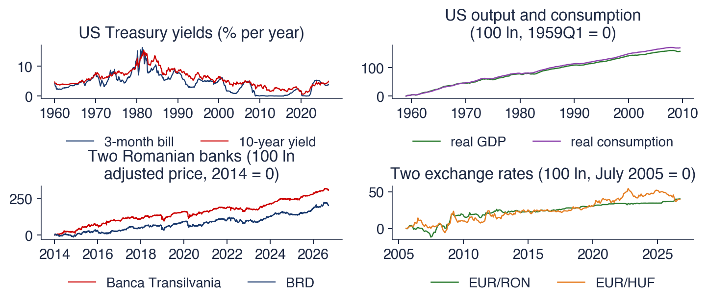

 TSA_ch7_common_trends