
Energy Markets Quantitative Analysis

Lecture 4: Risk Management for Energy Prices

Lecture 4

Risk Management for Energy Prices

Prof. dr. Daniel Traian PELE

Bucharest University of Economic Studies, Department of Statistics and Econometrics
Romanian Academy, Institute for Economic Forecasting

An energy company that buys or sells power every day does not lose money because prices are high; it loses money because tomorrow's price differs from the price it budgeted today. A supplier that buys 100 megawatts (MW) flat on the Romanian day-ahead market, Piața pentru Ziua Următoare (PZU), loses 2,400 euro (EUR) for every EUR per megawatt-hour (EUR/MWh) that the price rises above its budget. This lecture asks how large that loss can be on a bad day, how often a bad day comes, and how a company should turn the answer into limits, cash buffers and bank guarantees.

The two standard answers are value-at-risk (VaR), a high quantile of tomorrow's loss, and expected shortfall (ES), the average loss beyond that quantile. Lecture 1 promised to show why the normal curve understates crisis days; here we do it on real prices. We estimate VaR and ES in four ways on Romanian day-ahead prices from 1 Jan 2015 to 31 Oct 2026, check every method day by day over almost ten years (backtesting), and then follow the same quantiles into exchange margins, the day-ahead guarantee required by the market operator and position limits in MW.

The data are real and downloaded: the day-ahead base prices of Romania and of the Germany–Luxembourg zone, the Romanian load, the Brent crude oil futures and the Dutch gas price. The lecture ends with a case study of the price rise of autumn 2026, in which the danger turned out to be cash, not the daily VaR.

Learning outcomes

  • Measure the price risk of an energy position with VaR and ES, defined as quantiles of the loss distribution, and explain why the normal curve understates crisis days.
  • Estimate VaR and ES in four ways on Romanian prices: historical simulation, normal and Student-t curves, filtered historical simulation and extreme value theory.
  • Check a risk model after the fact with the Kupiec and Christoffersen tests, the Basel traffic light and a test for ES.
  • Turn quantiles into decisions: position limits, exchange margins and the day-ahead guarantee, for a supplier, a producer and a trader.

Lecture plan

  1. Price risk: losses, quantiles, VaR and ESThe risk of an energy position sits in the daily change of the price, and VaR and ES are two ways of summarising the bad tail of that change.
  2. Estimating VaR and ES: four methodsThere are many ways to estimate a quantile of tomorrow's loss, and on the same day and the same data they give different answers.
  3. Backtesting VaR and ESA VaR is a promise about how often losses will exceed it, and the promise can be checked after the fact.
  4. Margins, guarantees and position limitsThe quantiles of the previous sections become cash and limits in three places: the margins of an exchange, the guarantee of the day-ahead market and the position limits of a trading desk.
  5. Price risk for suppliers and producersA supplier and a producer face the same price but opposite tails, and a supplier's monthly bill adds the shape of its load.
  6. Case study: the price rise of autumn 2026In 2026 the Romanian price doubled between June and October without a single violent day.
  7. Wrap-upThe wrap-up tests the main ideas with five short questions, summarises the lecture and points to the research of our group and to further reading.
  8. AppendixThe appendix gives the derivations behind the ES formulas of the normal, Student-t and generalised Pareto curves, the backtests in full and the backtest table for Germany–Luxembourg.

Price risk: losses, quantiles, VaR and ES

The risk of an energy position sits in the daily change of the price, and VaR and ES are two ways of summarising the bad tail of that change. This section defines the loss, the two risk measures and shows on Romanian data why a limit built on the normal curve fails.

Data sources: prices and positions analysed

Slide 5 in the PDF

The main series is the day-ahead base price of Romania (RO) on the PZU, run by the Romanian electricity and gas market operator (OPCOM), with the price of the Germany–Luxembourg bidding zone (DE-LU) from the EPEX SPOT power exchange (EPEX) for comparison. Both come from the European Network of Transmission System Operators for Electricity (ENTSO-E) through energy-charts.info, the data portal of the Fraunhofer Institute for Solar Energy Systems (ISE), at daily and hourly frequency. The Romanian load, from ENTSO-E (Transelectrica data), gives the hourly shape of a supplier's portfolio. Two further series show how risk turns into cash: the front-month Brent crude oil futures, a margined contract, from Yahoo Finance (BZ=F), and the monthly gas price at the Dutch Title Transfer Facility (TTF), from the World Bank Pink Sheet.

The data run from 1 Jan 2015 to 31 Oct 2026, the last complete month, and were downloaded on 4 Nov 2026. The daily price is the mean of the delivery day in Central European Time (CET). Five missing days of the Romanian price stay missing, and the changes next to them are not computed. The backtest covers every day from 1 Jan 2017 to 31 Oct 2026, 3,587 valid days, and each forecast is made only with data up to the previous day, as a risk desk would have to do.

Daily price changes before and after 2021

Slide 7 in the PDF

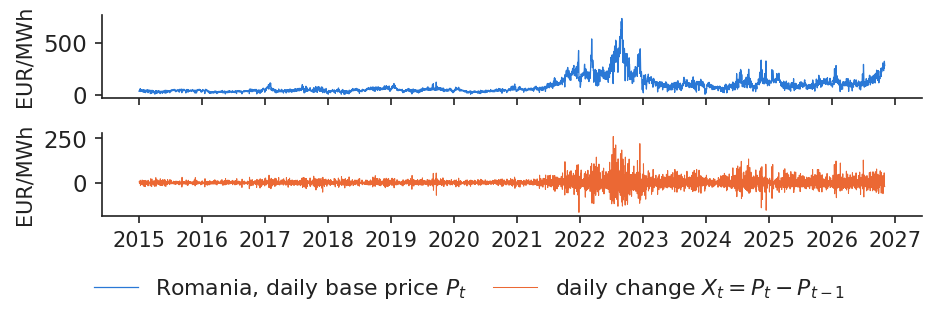
The variable that drives the loss is the change of the daily base price, \(X_t=P_t-P_{t-1}\), in EUR/MWh, where \(P_t\) is the base price of day \(t\). Power prices can be negative, so the lecture works with changes in euro rather than with log returns, which are not defined for a negative price.

The chart shows that the size of these changes is not stable. Until 2021 the daily changes are small; with the energy crisis they become violent, and they stay larger than before afterwards. The largest rise in the sample is 260.77 EUR/MWh, on 11 Jul 2022, and the largest fall is −166.59 EUR/MWh, on 24 Dec 2021. For a position of 100 MW flat, that is 2,400 MWh per day, every EUR/MWh of change moves the result of the day by 2,400 EUR.

In practice: a supplier that buys 100 MW flat on the PZU and budgets at yesterday's price loses 2,400 EUR for every EUR/MWh of rise.
Chart: Daily price changes before and after 2021

Daily change of the Romanian day-ahead base price, in EUR/MWh, 2015–2026.

Source: energy-charts.info (Fraunhofer ISE); OPCOM day-ahead prices for Romania, via ENTSO-E; own estimates. Data: daily, 2015-01-01 to 2026-10-31 (CET delivery days).

Value-at-risk is a quantile of tomorrow's loss

Slide 8 in the PDF

VaR is the loss that is exceeded only on a small, chosen share of days, for example one day in a hundred. For a buyer of \(Q\) MW flat, the loss of day \(t\) and its VaR are

\[L_t = Q\cdot 24\cdot X_t, \qquad \text{VaR}_{\alpha,t}=\min\{\ell:\ \Pr(L_t\le \ell\mid\mathcal F_{t-1})\ge\alpha\}\]
(4.1)

where \(L_t\) is the loss in EUR, \(Q\) the position in MW (for 100 MW flat, \(Q\cdot 24\) = 2,400 MWh per day), \(X_t\) the price change in EUR/MWh, \(\alpha\) the confidence level, 0.95 or 0.99, and \(\mathcal F_{t-1}\) the information available up to day \(t-1\), that is the prices known at 12:00 CET, the gate closure of the auction. VaR is therefore the \(\alpha\)-quantile of the loss, conditional on what is known when the bid is placed.

On the last 365 days of Romanian data, the 99% quantile of \(X_t\) is 86.63 EUR/MWh, which gives a VaR\(_{0.99}\) of 207,922 EUR for 100 MW; the 95% quantile is 50.39 EUR/MWh. What VaR does not say is how large the loss is on the worst 1% of days. It is a threshold, not an average, and for the size of the bad days we need ES.

In practice: the desk reports the 99% VaR every morning, before bidding at 12:00 CET.

Expected shortfall: the average loss beyond VaR

Slide 9 in the PDF

ES answers the question: when a bad day comes, how large is the loss on average? It is the mean of the loss beyond VaR, or equivalently the average of all VaRs above the level \(\alpha\):

\[\text{ES}_{\alpha,t}=\E\big[L_t\mid L_t\ge \text{VaR}_{\alpha,t}\big]=\frac{1}{1-\alpha}\int_{\alpha}^{1}\text{VaR}_{u,t}\,du\]
(4.2)

where \(u\) runs over the confidence levels above \(\alpha\). ES is a coherent risk measure (Artzner et al., 1999): in particular it is subadditive,

\[\text{ES}(L_1+L_2)\le\text{ES}(L_1)+\text{ES}(L_2)\]
(4.3)

where \(L_1\) and \(L_2\) are the losses of two positions, so diversification never adds risk. VaR may break this property (Acerbi and Tasche, 2002). This is why the Fundamental Review of the Trading Book (FRTB), the Basel market-risk rules, uses ES at 97.5% instead of VaR at 99% (BCBS, 2019).

On the last 365 days, VaR\(_{0.975}\) is 61.96 EUR/MWh and ES\(_{0.975}\) is 86.91 EUR/MWh, the mean of the 10 worst days. For 100 MW in Romania and 100 MW in Germany–Luxembourg, the 99% VaRs are 86.63 and 91.76 EUR/MWh separately but 150.77 together: with a correlation of 0.55 between the two price changes, the joint risk is smaller than the sum.

In practice: size the cash buffer with ES, not with VaR.

Large price rises are far more frequent than the normal curve allows

Slide 10 in the PDF

If price changes followed a normal curve, extreme days would be extremely rare. They are not. The excess kurtosis of \(X_t\) is 12.0 in Romania and 12.1 in Germany–Luxembourg, against 0 for a normal curve: the distribution has a narrow centre and long tails.

The count of large rises makes the point concrete. Rises above 3 standard deviations occurred on 52 days, while the normal curve expects 5.8 over the same sample. The largest rise is 10.1 standard deviations: under normality, such a day would come once in more than \(10^{20}\) years. The chart compares the observed distribution of changes with the normal curve fitted to the same mean and standard deviation, for both bidding zones.

In practice: a limit built on the normal curve understates how often a crisis day comes (Lecture 1).

Interactive chartInteractive page →

    Code of this chart: EMQA_L4_tails · open in Colab

    Distribution of daily price changes in Romania and Germany–Luxembourg, 2015–2026, against the normal curve with the same mean and standard deviation.

    Source: energy-charts.info (Fraunhofer ISE); OPCOM (RO) and EPEX SPOT (DE-LU) day-ahead prices, via ENTSO-E. Data: daily changes, 2015-01-01 to 2026-10-31.

    Question for the room A normal curve fitted to the Romanian daily price changes of 2015–2026 puts the 99% quantile at 60.18 EUR/MWh. The empirical 99% quantile is 88.21 EUR/MWh. Why the gap?
    Answer

    The daily changes have fat tails: excess kurtosis 11.97, and 52 rises above three standard deviations against 5.82 expected under the normal law. The normal VaR therefore understates the extreme quantiles, and the gap widens as α grows. ES (the mean loss beyond VaR) reacts even more, because it averages the extreme days the normal curve misses. Choose the period 2021–2022 to see both measures on the crisis years, or the last 365 days for the current risk.

    A normal-curve limit set in 2020 was breached 19 times more often than planned in 2021–2022

    Slide 11 in the PDF

    A static limit assumes that tomorrow's risk looks like the past; in a crisis it does not. Consider the limit a risk manager would have set at the end of 2020 from the normal curve:

    \[\ell_{0.99}=\hat\mu+z_{0.99}\,\hat\sigma, \qquad z_{0.99}=2.326\]
    (4.4)

    where \(\hat\mu\) and \(\hat\sigma\) are the mean and standard deviation of \(X_t\) in 2015–2020 and \(z_{0.99}\) is the 99% quantile of the standard normal distribution. A correct limit is exceeded on 1% of days.

    Estimated on 2,182 days of 2015–2020, \(\hat\sigma\) is 10.21 and the limit is 23.77 EUR/MWh. Already within 2015–2020 it was breached 45 times against 21.8 expected, because of the fat tails. Afterwards the failure became dramatic: 139 breaches in 2021–2022 against 7.3 expected, and 226 in 2023–2026 against 14.0 expected, 16 times more. The limit did not move when volatility moved, so it measured a market that no longer existed.

    In practice: a limit must move with volatility; the next section shows four ways to make it move.

    Estimating VaR and ES: four methods

    There are many ways to estimate a quantile of tomorrow's loss, and on the same day and the same data they give different answers. This section presents historical simulation, the normal and Student-t curves, filtered historical simulation and extreme value theory, then compares them on October 2026 and through the 2021–2022 crisis.

    Historical simulation with a one-year window

    Slide 13 in the PDF

    Historical simulation (HS) assumes no distribution: it sorts the last 365 daily changes and reads the quantile directly; the 4th largest change is the 99% VaR. Formally,

    \[\widehat{\text{VaR}}^{\text{HS}}_{\alpha,t}=\hat q_{\alpha}\big(X_{t-W},\dots,X_{t-1}\big), \qquad \widehat{\text{ES}}^{\text{HS}}_{\alpha,t}=\text{mean of }\{X_s\ge\widehat{\text{VaR}}^{\text{HS}}_{\alpha,t}\}\]
    (4.5)

    where \(W\) = 365 days is the window, \(\hat q_\alpha\) the empirical quantile of the changes in the window, and \(X_s\) the changes of the window that lie at or above the VaR.

    On October 2026, HS gives a VaR\(_{0.99}\) of 86.63 and an ES\(_{0.975}\) of 87.59 EUR/MWh. Over the backtest 2017–2026 it was exceeded on 2.04% of days, not on 1%. Its weakness is speed: a new regime needs months to fill the window, and a crisis day counts with full weight for 365 days, then drops out at once, so the VaR jumps down on a fixed date that has nothing to do with the market.

    In practice: HS is the default in many energy companies, and it lags the market.

    Parametric VaR: normal and Student-t distributions

    Slide 14 in the PDF

    The parametric approach fits a curve to the last year of changes and reads its quantile. The normal curve has two parameters; the Student-t curve adds a third, the degrees of freedom, which makes its tails fatter:

    \[\text{VaR}^{N}_{\alpha}=\mu+\sigma z_\alpha, \qquad \text{ES}^{N}_{\alpha}=\mu+\sigma\frac{\varphi(z_\alpha)}{1-\alpha}\]
    (4.6)
    \[\text{VaR}^{t}_{\alpha}=m+s\,t_{\nu,\alpha}, \qquad \text{ES}^{t}_{\alpha}=m+s\,\frac{g_\nu(t_{\nu,\alpha})}{1-\alpha}\cdot\frac{\nu+t_{\nu,\alpha}^2}{\nu-1}\]
    (4.7)

    where \(\mu\) and \(\sigma\) are the mean and standard deviation, \(z_\alpha\) and \(\varphi\) the quantile and density of the standard normal distribution, \(m\), \(s\) and \(\nu\) the location, scale and degrees of freedom of the Student-t curve, estimated by maximum likelihood estimation (MLE), and \(t_{\nu,\alpha}\) and \(g_\nu\) the Student-t quantile and density. The ES formulas are derived in Appendix A.

    On October 2026 the normal curve gives VaR\(_{0.99}\) 69.64 and ES\(_{0.975}\) 69.98 EUR/MWh; the Student-t gives 76.66 and 80.05. In the backtest the normal 99% VaR was exceeded on 3.21% of days and the Student-t on 1.98%, against a target of 1%. The t curve fixes part of the tail but not the centre: at 95% it is too narrow, with 8.75% of days above it.

    In practice: the normal VaR is the easiest to explain and the most dangerous to trust.

    Filtered historical simulation: past shocks rescaled to current volatility

    Slide 15 in the PDF

    Filtered historical simulation (FHS) combines the two previous ideas. It divides past changes by their volatility to obtain standardised shocks, then rescales those shocks by today's volatility, so that the shape of the tail comes from history and the scale from the present (Barone-Adesi, Giannopoulos and Vosper, 1999):

    \[e_t=X_t-\mu_{d(t)}, \quad \sigma_t^2=\omega+a\,e_{t-1}^2+b\,\sigma_{t-1}^2, \quad z_t=e_t/\sigma_t\]
    (4.8)
    \[\text{VaR}^{\text{FHS}}_{\alpha,t}=\mu_{d(t)}+\sigma_t\,\hat q_\alpha(z)\]
    (4.9)

    where \(\mu_{d(t)}\) is the mean change of that weekday (prices fall at weekends), \(e_t\) the change net of that mean, \(\sigma_t\) the generalised autoregressive conditional heteroskedasticity (GARCH) volatility of Lecture 3 (Bollerslev, 1986) with parameters \(\omega\), \(a\) and \(b\), refitted every 21 days on 730 days, \(z_t\) the standardised shock and \(\hat q_\alpha(z)\) the empirical quantile of the shocks. ES is \(\sigma_t\) times the mean of the shocks \(z\) above \(\hat q_\alpha(z)\).

    On the Romanian data the GARCH(1,1) volatility ranges from 4.06 EUR/MWh (29 Mar 2021) to 100.86 EUR/MWh (12 Jul 2022). In October 2026, the FHS VaR\(_{0.99}\) is 67.50 EUR/MWh. In the backtest, the 99% VaR was exceeded on 1.51% of days, and the 95% VaR on 5.58%, with a Kupiec \(p\)-value of 0.120: the first method so far that passes at 95%.

    In practice: FHS raises the limit within days of a volatility jump; HS needs months.

    Extreme value theory: model only the tail, with a generalised Pareto curve

    Slide 16 in the PDF

    Extreme value theory (EVT) models only the tail. Above a high threshold, the excesses of almost any distribution follow the same two-parameter curve, the generalised Pareto distribution (GPD) (Pickands, 1975):

    \[\Pr(Z-u\le y\mid Z>u)\approx 1-\Big(1+\frac{\xi y}{\beta}\Big)^{-1/\xi}\]
    (4.10)
    \[\text{VaR}_\alpha=u+\frac{\beta}{\xi}\Big[\Big(\frac{n}{N_u}(1-\alpha)\Big)^{-\xi}-1\Big], \quad \text{ES}_\alpha=\frac{\text{VaR}_\alpha+\beta-\xi u}{1-\xi}\]
    (4.11)

    where \(Z\) is the standardised shock, \(y\) the excess over the threshold, \(u\) the threshold, chosen by the peaks-over-threshold (POT) method as the 90% quantile of \(z\), \(N_u\) the number of the \(n\) residuals that exceed it, \(\xi\) the shape (tail heaviness) and \(\beta\) the scale of the GPD, both estimated by MLE. The result is then multiplied by \(\sigma_t\) as in FHS (McNeil and Frey, 2000); the derivation is in Appendix B.

    On raw changes, with the threshold at the 95% quantile, \(\hat\xi\) = 0.164: a heavy tail, in which moments above order 6.1 do not exist. After the GARCH filter, the median \(\hat\xi\) is 0.011: the filter absorbs most of the tail. In the backtest the 99% EVT VaR was exceeded on 1.37% of days, the best of the five methods.

    In practice: use EVT for the one-in-ten-years day that no window contains.

    Above the threshold the Pareto curve fits the data; the normal curve does not

    Slide 17 in the PDF

    The chart shows the tail of the GARCH-filtered changes over the 730 days before 31 Oct 2026 together with the fitted Pareto curve and the normal curve. At the last refit, on 11 Oct 2026, the estimates are \(\hat\xi\) = 0.182 and \(\hat\beta\) = 0.569. Above the threshold the Pareto curve follows the observed points, while the normal curve falls off far too quickly.

    The shape parameter is not stable: \(\hat\xi\) was positive in 53% of the refits, so the standardised tail is sometimes heavy and sometimes not (Balkema and de Haan, 1974; McNeil and Frey, 2000). This is one reason to refit the model regularly rather than fix a tail shape once.

    In practice: a 4-sigma day is rare but not impossible; the normal curve calls it impossible.

    Interactive chartInteractive page →

      Code of this chart: EMQA_L4_gpd_tail · open in Colab

      Tail of the GARCH-filtered Romanian price changes over the 730 days before 31 Oct 2026, with the fitted generalised Pareto curve and the normal curve.

      Source: energy-charts.info (Fraunhofer ISE); OPCOM day-ahead prices for Romania, via ENTSO-E; own estimates. Data: GARCH-filtered changes, the 730 days before 2026-10-31.

      Question for the room The generalised Pareto distribution (GPD) is fitted to the residuals above the threshold u. Does the estimated tail shape ξ depend on the choice of u?
      Answer

      Yes, and this is the main practical difficulty of extreme value theory (EVT): a low threshold gives many exceedances but mixes in the body of the distribution; a high threshold uses only a few dozen points and the estimate becomes noisy. Move u from 80% to 97% and watch ξ and the implied 99.9% quantile. In the lecture, the shape at the 90% threshold varies between −0.38 and 0.33 across the 171 refits since 2017, positive in 53% of them.

      VaR and ES on the same day by five methods

      Slide 18 in the PDF

      The table gives the mean of the 31 forecasts made for October 2026. The first three columns are in EUR/MWh; the last two are in thousand EUR for 100 MW flat, 2,400 MWh per day.

      MethodVaR 0.95VaR 0.99ES 0.975VaR 0.99, kEURES 0.975, kEUR
      HS50.3886.6387.59208210
      Normal49.3369.6469.98167168
      Student-t45.7776.6680.05184192
      FHS36.2267.5067.44162162
      EVT35.6664.3368.54154164

      The same position, on the same day, has a 99% VaR between 154 and 208 thousand EUR depending on the method. The gap is not noise. HS and Student-t still carry the volatile days of the past year in their window, while FHS and EVT use today's volatility, which in October 2026 was below the yearly average. Choosing a method is therefore a risk decision in its own right.

      In practice: report two methods side by side and explain the gap.

      In the crisis FHS adapted within days; HS and the normal VaR lagged

      Slide 19 in the PDF

      The difference between methods matters most in a crisis. Between 1 Jul 2021 and 30 Jun 2023, 730 days, a correct 99% VaR should have been exceeded 7.3 times. The counts were 28 for HS, 45 for the normal curve, 29 for the Student-t, 19 for FHS and 17 for EVT. No method was right, but the filtered ones, which follow the GARCH volatility, adapted within days, while HS and the normal VaR waited for their windows to fill with crisis days.

      In practice: in a crisis, a model that reacts within days protects the cash.

      Interactive chartInteractive page →

        Code of this chart: EMQA_L4_var_paths · open in Colab

        Daily price changes in Romania and the 99% VaR forecasts of the five methods, 1 Jul 2021 to 30 Jun 2023, with the exceedances marked.

        Source: energy-charts.info (Fraunhofer ISE); OPCOM day-ahead prices for Romania, via ENTSO-E; own estimates. Data: forecasts for 2021-07-01 to 2023-06-30.

        Question for the room In July 2021–June 2023, a correct 99% VaR model should be exceeded on about 7 of the 730 days. How many exceedances do the normal model and filtered historical simulation (FHS) have?
        Answer

        The normal model is exceeded on 45 days, historical simulation (HS) on 28, FHS on 19 and EVT on 17 (expected 7.3). All methods were too low in the crisis, but FHS, which scales the residuals by a GARCH (generalised autoregressive conditional heteroskedasticity) volatility, reacts within days to a volatility jump, while HS and the normal model, with a 365-day window, adapt only slowly. The Kupiec test in the readout compares the exceedance rate of the window with 1 − α.

        The square-root-of-time rule overstates the 10-day risk

        Slide 20 in the PDF

        Regulators and many companies scale a one-day VaR to ten days by multiplying it by \(\sqrt{10}\) = 3.16. The rule assumes that daily changes are independent, like a random walk. Power prices are not: they revert to a level set by fuel costs and the weekly calendar.

        Measured directly, the 10-day 99% quantile is 1.72 times the 1-day one in Romania and 1.75 times in Germany–Luxembourg, not 3.16. The variance ratio at 10 days is 0.33, where 1 would mean a random walk. The autocorrelation of \(X_t\) is −0.076 at lag 1, a mild reversal, and 0.474 at lag 7, the weekly pattern (Weron, 2014). The chart compares the empirical quantile at each horizon with the square-root scaling.

        In practice: for a 10-day horizon, measure 10-day changes directly; multiplying by √10 wastes capital.

        Interactive chartInteractive page →

          Code of this chart: EMQA_L4_horizon · open in Colab

          Empirical 99% quantile of price changes over horizons up to 10 days, in Romania and Germany–Luxembourg, against the square-root-of-time scaling of the 1-day quantile.

          Source: energy-charts.info (Fraunhofer ISE); OPCOM (RO) and EPEX SPOT (DE-LU) day-ahead prices, via ENTSO-E. Data: daily base prices, 2015-01-01 to 2026-10-31.

          Question for the room The square-root-of-time rule scales a 1-day VaR to 10 days by √10 = 3.16. What ratio do the Romanian prices show at the 99% level?
          Answer

          Only 1.72 (Germany–Luxembourg: 1.75). Daily price changes are negatively autocorrelated (ρ(1) = −0.076): a price spike is followed by a fall, so changes over several days partly cancel. The variance ratio at 10 days is 0.33, far below 1. The √h rule assumes independent changes and would overstate the 10-day VaR of a flat day-ahead position.

          Backtesting VaR and ES

          A VaR is a promise about how often losses will exceed it, and the promise can be checked after the fact. This section counts exceedances with the Kupiec test, checks their timing with the Christoffersen test and the Basel traffic light, and tests ES with the Acerbi–Székely statistic, over 3,587 days.

          Kupiec test of the exceedance frequency

          Slide 22 in the PDF

          A 99% VaR promises to be exceeded on 1% of days. The Kupiec (1995) test counts the exceedances and tests whether their share differs from that promise:

          \[I_t=\mathbf 1\{L_t>\text{VaR}_{\alpha,t}\}, \qquad x=\textstyle\sum_{t=1}^{n}I_t, \qquad \hat p=x/n\]
          (4.12)
          \[\text{LR}_{uc}=-2\ln\frac{(1-p)^{n-x}\,p^{x}}{(1-\hat p)^{n-x}\,\hat p^{\,x}}\ \sim\ \chi^2_1\]
          (4.13)

          where \(I_t\) is the exceedance indicator (1 if the loss exceeds the VaR, 0 otherwise), \(n\) the number of days, \(x\) the number of exceedances, \(\hat p\) their observed share and \(p=1-\alpha\) the promised share. \(\text{LR}_{uc}\) is the likelihood ratio (LR) test of unconditional coverage; under the null hypothesis it follows a \(\chi^2\) distribution with one degree of freedom, and the model is rejected at 5% if \(\text{LR}_{uc}\) exceeds 3.84.

          For the 99% VaR on 3,587 days, 35.9 exceedances are expected. The normal VaR had 115, with \(\text{LR}_{uc}\) = 111.5; FHS had 54, with \(\text{LR}_{uc}\) = 8.0; EVT had 49, with \(p\) = 0.037. The power of the test depends on the sample: with one year at 99% we expect only 2–3 exceedances, and the test can hardly reject anything; ten years of daily data make it sharp.

          In practice: ask for the exceedance count before you trust anyone's VaR.

          Christoffersen test of independent exceedances

          Slide 23 in the PDF

          A good model is not surprised twice in a row: an exceedance today should not make one tomorrow more likely. Christoffersen (1998) tests this by comparing two conditional probabilities:

          \[\pi_{01}=\Pr(I_t=1\mid I_{t-1}=0), \qquad \pi_{11}=\Pr(I_t=1\mid I_{t-1}=1)\]
          (4.14)
          \[\text{LR}_{ind}=-2\ln\frac{(1-\hat\pi)^{n_{00}+n_{10}}\hat\pi^{\,n_{01}+n_{11}}}{(1-\hat\pi_{01})^{n_{00}}\hat\pi_{01}^{\,n_{01}}(1-\hat\pi_{11})^{n_{10}}\hat\pi_{11}^{\,n_{11}}}\sim\chi^2_1\]
          (4.15)

          where \(\pi_{01}\) is the probability of an exceedance after a quiet day, \(\pi_{11}\) the probability of an exceedance after an exceedance, \(n_{ij}\) the number of days with \(I_{t-1}=i\) and \(I_t=j\), \(\hat\pi\) the overall share of exceedances and \(\hat\pi_{01}\), \(\hat\pi_{11}\) the estimated conditional shares. The null hypothesis is \(H_0\): \(\pi_{01}=\pi_{11}\). The joint test of coverage and independence is \(\text{LR}_{cc}\) = \(\text{LR}_{uc}\) + \(\text{LR}_{ind}\), distributed as \(\chi^2_2\).

          On the 99% VaR the independence \(p\)-values are 0.682 for HS, 0.868 for the normal VaR and 0.199 for FHS. No method fails: exceedances rarely fall on consecutive days. But they do cluster in months. The normal VaR was exceeded on 7.26% of days in 2021–2022 and on 2.33% in 2017–2020. A first-order test, which only looks at yesterday, misses this; the traffic light, which looks at a 250-day window, sees it.

          In practice: look at the timing of exceedances, not only at their number.

          Over ten years only the filtered methods pass at 95%; at 99% every method has too many exceedances

          Slide 24 in the PDF

          The table collects the backtest of all five methods on Romania, 1 Jan 2017 to 31 Oct 2026. The expected shares are 5% and 1% of 3,587 days, that is 35.9 exceedances at 99%. "Red days" is the share of days whose last 250 days held 10 or more exceedances (next block); the same table for Germany–Luxembourg is in Appendix D.

          Romania95%: shareKupiec p99%: countshare, %Kupiec pChristoffersen pred days, %
          HS6.160.002732.04<0.0010.68216.7
          Normal7.36<0.0011153.21<0.0010.86829.5
          Student-t8.75<0.001711.98<0.0010.63018.3
          FHS5.580.120541.510.0050.1996.2
          EVT5.550.139491.370.0370.2442.8

          At 95% only FHS and EVT pass the Kupiec test, with \(p\)-values of 0.120 and 0.139. At 99% every method is rejected, but the gap is very different: the normal VaR is exceeded on 3.21% of days and spends 29.5% of days in the red zone, while EVT is exceeded on 1.37% and is red on 2.8% of days. No method captures the 99% tail of power prices fully.

          In practice: accept a model at 95%, but hold extra capital for the 99% tail that none of them captures fully.

          The Basel traffic light: the normal VaR spent 30% of days in the red zone

          Slide 25 in the PDF

          The Basel Committee on Banking Supervision (BCBS, 1996) judges a 99% VaR by the count of exceedances in the last 250 days: green for 0–4, yellow for 5–9 and red for 10 or more. A correct model is green with probability 89.2% and red with probability 0.025%, so a red zone is strong evidence that the model is wrong.

          The chart follows the zone of each method day by day through the backtest. The normal VaR spent almost a third of the days in the red zone; HS was red on 16.7% of days, FHS on 6.2% and EVT on 2.8%. The red periods are concentrated in the crisis years, which is the clustering in months that the Christoffersen test did not detect.

          In practice: yellow means recalibrate, red means stop using the model for limits.

          Interactive chartInteractive page →

          Methods

            Code of this chart: EMQA_L4_traffic · open in Colab

            Basel traffic-light zone of each method's 99% VaR (count of exceedances in the last 250 days), Romania, backtest 2017–2026.

            Source: energy-charts.info (Fraunhofer ISE); OPCOM day-ahead prices for Romania, via ENTSO-E; own estimates. Data: backtest 2017-01-01 to 2026-10-31, 99% VaR.

            Question for the room Over 250 days, a correct 99% VaR model is in the green zone (at most 4 exceedances) 89.2% of the time. In which share of the days is the normal model in the red zone (10 or more)?
            Answer

            In 29.5% of the days since the backtest window filled (from September 2017), against 6.2% for FHS and 2.8% for EVT; a correct model would be red only 0.025% of the time. The zones are binomial quantiles: green while the cumulative probability of the count under a Binomial(n, 1%) law is below 95%, red from 99.99%. Change the window to see the thresholds scale with n.

            Exceedance rates by method in 2021–2022 and since 2023

            Slide 26 in the PDF

            Splitting the backtest into three periods shows where the failures come from. The table gives the share of days above the 99% VaR, in percent, for Romania and Germany–Luxembourg.

            99% VaR, % of daysRO 17–20RO 21–22RO 23–26DE-LU 17–20DE-LU 21–22DE-LU 23–26
            HS1.584.931.001.163.841.07
            Normal2.337.262.002.405.892.07
            Student-t1.304.661.291.373.971.29
            FHS1.372.880.931.442.471.36
            EVT1.242.470.931.512.191.07

            In the crisis even FHS was exceeded on 2.88% of days in Romania: the gas shock moved the whole distribution, not only its scale. After the crisis the picture changes: since 2023, FHS and EVT are at 0.93%, HS at 1.00% and only the normal VaR stays far off, at 2.00%. A model that looks good on calm years tells little about its behaviour in a crisis.

            In practice: test every model on 2021–2022 before you trust it in a crisis.

            Backtesting ES: the size of losses beyond VaR

            Slide 27 in the PDF

            ES cannot be checked by counting, because it is a statement about the size of the losses beyond VaR. Acerbi and Székely (2014) divide each exceedance loss by its ES forecast; if ES is right, these ratios average 1:

            \[Z_2=\frac{1}{T(1-\alpha)}\sum_{t=1}^{T}\frac{L_t\,I_t}{\text{ES}_{\alpha,t}}-1, \qquad \E_{H_0}[Z_2]=0\]
            (4.16)

            where \(T\) is the number of days, \(\alpha\) = 0.975, \(I_t\) the exceedance of VaR\(_{0.975}\), \(L_t\) the loss and \(\text{ES}_{\alpha,t}\) the ES forecast. A positive \(Z_2\) means that ES was too small. The \(p\)-value comes from 2,000 paths simulated from each model (Appendix C).

            Z2allp2021–22p2023–26p
            HS0.628<0.0012.694<0.001−0.0260.761
            Normal1.425<0.0014.170<0.0010.697<0.001
            Student-t0.908<0.0012.910<0.0010.3290.052
            FHS0.3350.0041.164<0.001−0.0830.759
            EVT0.2790.0091.183<0.001−0.1140.722

            Every ES was too small in the crisis, the normal one by the widest margin. Since 2023, FHS, EVT and HS pass. Because a 97.5% ES rests on only about 9 tail days a year, its comparison needs several years of data (Pele and Mazurencu-Marinescu-Pele, 2026).

            In practice: judge ES on several years, never on one quarter (about 9 tail days a year).

            AIDA 2026: a conformal shift measures and corrects the miscalibration of VaR

            Slide 28 in the PDF

            At the AIDA conference (Bucharest University of Economic Studies, 4 June 2026), D. T. Pele presented joint work with V. Bolovăneanu, A. T. Ginavar, S. Lessmann and W. K. Härdle on recalibrating VaR forecasts (slides; the paper is submitted). The method needs a single number. Each day the score \(s_t=\hat q_t-r_t\) compares the forecast quantile with the realised return and is positive on an exceedance day; \(\hat q_V\) is the 99% quantile of past scores, and the corrected VaR is the VaR plus \(\hat q_V\). The shift is either fixed on a calibration sample (an audit) or rolled over the last 250 days (for daily use). The work applies it to the 1% VaR of 10 models, foundation models, GARCH-type models and HS, on 24 assets including oil and gas, 240 pairs in all, and judges the result with the Kupiec and Christoffersen tests and the traffic light of this section.

            As a diagnosis, \(\hat q_V\) ranges from −0.007, for a model that is too prudent, to +0.102, for a model with no usable tail signal, and it explains 53.4% (partial \(R^2\)) of the gain in quantile score. As a repair, the green-zone pairs rise from 63/240 (26.2%) raw to 203/240 (84.6%) with the fixed shift and 234/240 (97.5%) with the rolling shift. The exceedance rate is restored, but their clustering is not, so the Christoffersen test keeps its role. The link to this lecture is direct: Kupiec says whether VaR fails, \(\hat q_V\) says by how much, and the widening \(\hat c_t\) of the day-ahead guarantee in the next section is the same one-parameter shift.

            In practice: after a failed backtest, widen VaR by the conformal shift and keep testing for clusters.

            Margins, guarantees and position limits

            The quantiles of the previous sections become cash and limits in three places: the margins of an exchange, the guarantee of the day-ahead market and the position limits of a trading desk. This section shows how each is computed and why a well-hedged company can still run out of cash.

            Exchange margins: initial margin as a VaR, variation margin paid daily

            Slide 30 in the PDF

            A clearing house holds a deposit that covers a 99% two-day loss and settles gains and losses in cash every evening:

            \[\text{IM}_t=K F_t\,\hat q_{0.99}\big(|r^{(2)}|\big), \qquad \text{VM}_t=n K(F_t-F_{t-1})\]
            (4.17)

            where \(\text{IM}_t\) is the initial margin (IM) and \(\text{VM}_t\) the variation margin (VM), both set by the central counterparty (CCP), \(F_t\) the futures price, \(K\) = 1,000 barrels per Brent lot, \(r^{(2)}\) the two-day return, \(\hat q_{0.99}\) its empirical 99% quantile in absolute value and \(n\) the number of lots sold (positive) or bought (negative).

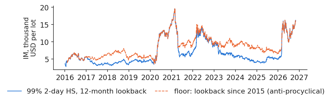
            The rules come from the European Market Infrastructure Regulation (EMIR) and its regulatory technical standards (RTS), Delegated Regulation 153/2013. For futures, the margin must cover 99% of losses over a 2-day liquidation period, on at least 12 months of data (Art. 24–26). Article 28 adds anti-procyclicality (APC) tools: a 25% buffer, a 25% weight on stressed observations, or a floor computed on 10 years. On the Intercontinental Exchange (ICE) Brent contract, a position of 100 lots sold faced its largest one-day VM of 0.88 million United States dollars (USD) on 16 Sep 2019.

            In practice: a hedged producer gains on the physical sale later, but pays the margin today.

            Margin calls and liquidity shortfalls of hedged energy companies in 2022

            Slide 31 in the PDF

            The European Central Bank (ECB) described what happened in November 2022. TTF gas futures reached 227 EUR/MWh on 7 March 2022, about 12 times the level of early 2021. By mid-2022 about twice as much initial margin was posted as in late 2021. The firms hurt were mostly utilities and producers that had sold forward: hedgers, not speculators. Their physical position gained value, but the gain would arrive only at delivery, while the margin had to be paid in cash immediately.

            The European Union (EU) responded with Delegated Regulation (EU) 2022/2311, which accepted public guarantees as collateral until 29 November 2023. In Romania the same mechanism works on the day-ahead market: OPCOM accepts a buy order at a positive price only up to the participant's guarantee, usually a bank letter (OPCOM, 2025).

            In practice: the risk that sinks a hedged company is liquidity, not the price itself.

            Margins are procyclical: in 2026 the Brent margin rose 2.7-fold in two months

            Slide 32 in the PDF

            A margin computed from the last 12 months of returns rises exactly when the market becomes volatile, which is when cash is scarcest. The chart recomputes the Brent initial margin per lot from the front-month futures. In early 2026 Brent rose from 72.48 USD on 27 Feb 2026 to 118.35 USD on 31 Mar 2026. With 12 months of history, the IM went from 5,970 to 16,313 USD per lot, ×2.73; with a floor computed on data since 2015, it rose only ×2.07.

            The floor also protects better: losses beyond the IM occurred on 1.80% of days with 12 months of history and on 0.66% with the floor, against a target of 1%. The anti-procyclicality tools of EMIR are therefore not only a matter of stability for the clearing house; they also make the margin a better 99% quantile.

            In practice: plan your cash for the margin a crisis would demand, not for today's margin.
            Chart: Margins are procyclical: in 2026 the Brent margin rose 2.7-fold in two months

            Brent front-month price and the initial margin per lot computed with 12 months of history and with a floor since 2015, trading days 2016–2026.

            Source: Yahoo Finance (ICE Brent front-month BZ=F); own computation. Data: trading days 2016-01-01 to 2026-10-30; contract-roll days dropped; 1 lot = 1,000 bbl.

            The day-ahead guarantee is set from a quantile forecast of tomorrow's price

            Slide 33 in the PDF

            To be sure its order clears, a supplier bids up to a high price, and the guarantee must cover price times volume. The guarantee therefore rests on a high quantile of tomorrow's price, forecast with quantile regression (QR) (Koenker and Bassett, 1978) and widened with a conformal correction (Romano et al., 2019):

            \[G_t\ \ge\ Q\cdot 24\cdot \hat q_{\tau,t}, \qquad \hat q_{\tau,t}=\beta_0+\beta_1P_{t-1}+\beta_2P_{t-7}+\textstyle\sum_j\delta_jD_{j,t}\]
            (4.18)
            \[\tilde q_{\tau,t}=\hat q_{\tau,t}+\hat c_t, \qquad \hat c_t=\hat q_\tau\big(P_s-\hat q_{\tau,s},\ s=t-365,\dots,t-1\big)\]
            (4.19)

            where \(G_t\) is the guarantee in EUR, \(Q\) the position in MW, \(\hat q_{\tau,t}\) the QR forecast of the \(\tau\)-quantile of the price, estimated on the last 365 days as in quantile regression averaging (QRA) of Lecture 2, \(\beta_0\), \(\beta_1\), \(\beta_2\) and \(\delta_j\) its coefficients, \(P_{t-1}\) and \(P_{t-7}\) the prices one day and one week earlier, \(D_{j,t}\) weekday dummies, \(\tilde q_{\tau,t}\) the widened quantile and \(\hat c_t\) the conformal correction, the \(\tau\)-quantile of the past forecast errors.

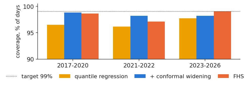
            With \(\tau\) = 0.99 over 2017–2026, the price stayed below the forecast on 96.90% of days with plain QR, 98.47% with the widened QR and 98.49% with FHS. For 100 MW flat the guarantee costs 0.371 million EUR per day on average, and the widening adds 7.5%. The amount depends strongly on the regime: 0.172 million EUR per day in 2017–2020 and 0.649 in 2021–2022.

            In practice: size the bank line behind the guarantee on the crisis quantile, before the crisis.

            Heavier tails bring the 99% quantile close to its nominal coverage

            Slide 34 in the PDF

            The chart compares, through the backtest, the share of days on which the price stayed below each 99% forecast. The Kupiec \(p\)-values at 99% are below 0.001 for plain QR, 0.003 for the widened QR and 0.005 for FHS: the conformal correction moves the coverage close to its promise, though not quite to it. At 95% the widened QR passes, with \(p\) = 0.053, as Lecture 2 suggested for the tails (Nowotarski and Weron, 2018).

            In practice: a forecast used for collateral must be calibrated in the tail, not only accurate on average.
            Chart: Heavier tails bring the 99% quantile close to its nominal coverage

            Coverage of the 99% quantile forecast of the Romanian day-ahead price for plain QR, the widened QR and FHS, backtest 2017–2026.

            Source: energy-charts.info (Fraunhofer ISE); OPCOM day-ahead prices for Romania, via ENTSO-E; own estimates. Data: forecasts 2017-01-01 to 2026-10-31, 99% quantile.

            A position limit in MW should shrink when VaR grows

            Slide 35 in the PDF

            The board sets a daily risk budget in EUR; the desk divides it by today's VaR per MW:

            \[Q^{\max}_t=\frac{B}{24\cdot\text{VaR}^{\text{FHS}}_{0.99,t}}\]
            (4.20)

            where \(B\) is the daily VaR budget, here 250,000 EUR (an assumption for the example), \(\text{VaR}^{\text{FHS}}_{0.99,t}\) the FHS 99% VaR in EUR/MWh and \(Q^{\max}_t\) the maximum open flat position in MW.

            With the FHS 99% VaR on Romanian data, the median VaR of 2019 was 20.27 EUR/MWh, which allows 514 MW. On 12 Jul 2022 the VaR was 245.80 and the limit only 42 MW. On 31 Oct 2026 the VaR was 53.15 and the limit 196 MW. A fixed MW limit lets the money at risk grow with volatility; a fixed EUR budget keeps it constant and forces the position to shrink when the market becomes dangerous.

            In practice: set limits in EUR of VaR and convert them to MW every day.

            Price risk for suppliers and producers

            A supplier and a producer face the same price but opposite tails, and a supplier's monthly bill adds the shape of its load. This section measures the supplier's monthly cash-flow-at-risk, compares the two tails and summarises case study C4 on systemic and energy-specific risks.

            A supplier's monthly cost-at-risk under the normal distribution

            Slide 37 in the PDF

            A supplier prices next month at this month's cost; the risk is a jump of the load-weighted price. The cost overrun and its quantile are

            \[\bar P^{L}_m=\frac{\sum_h P_hL_h}{\sum_h L_h}, \qquad o_m=\frac{\bar P^{L}_m}{\bar P^{L}_{m-1}}-1, \qquad \text{CFaR}_{0.95}=\hat q_{0.95}(o_m)\]
            (4.21)

            where \(P_h\) is the hourly price, \(L_h\) the Romanian load in hour \(h\) (the shape of the portfolio), \(\bar P^{L}_m\) the load-weighted price of month \(m\), \(o_m\) the cost overrun from one month to the next and the cash-flow-at-risk (CFaR) its quantile. Amounts in EUR are for a portfolio of 100 MW on average.

            Over 140 months, from Mar 2015 to Oct 2026, the normal 99% limit estimated on 2015–2020 is an overrun of +50.5%. It was exceeded 3 times since 2021, against 0.7 expected. The worst month was Nov 2024, with +86.6%, or 5.96 million EUR. Empirically, on all months, the CFaR\(_{0.95}\) is +39.9%, i.e. 2.84 million EUR, and the ES\(_{0.95}\) is +60.2%, i.e. 6.49 million EUR.

            In practice: price a fixed retail offer with an ES-based premium, or hedge it forward (Lecture 5).

            Since 2021 the normal 99% monthly limit was exceeded 3 times (0.7 expected)

            Slide 38 in the PDF

            The chart shows the monthly overrun of the load-weighted cost since March 2015 together with the normal 99% limit computed in 2020. The red bars are the months that exceed the limit. The largest overrun came in Nov 2024, after the summer of 2024, and not during the 2022 crisis: a supplier's monthly risk depends on the jump from one month to the next, not on the level of the price.

            In practice: re-estimate the monthly limit every quarter and stress it with the 2022 months.

            Interactive chartInteractive page →

              Code of this chart: EMQA_L4_supplier_month · open in Colab

              Monthly overrun of the load-weighted power cost in Romania, Mar 2015 to Oct 2026, with the normal 99% limit computed in 2020; months above the limit in red.

              Source: energy-charts.info (Fraunhofer ISE); OPCOM prices; ENTSO-E load (Transelectrica data for Romania). Data: monthly, 2015-03 to 2026-10.

              Question for the room A supplier budgets each month at the load-weighted price of the previous month. A normal 99% limit estimated on 2015–2020 puts the monthly cost overrun at 50.5%. How many months exceed it in 2021–2026?
              Answer

              Three months out of 70, against 0.7 expected; the worst is November 2024, +86.6% (about 5.96 million EUR for 100 MW shaped like the national load). The limit estimated on calm years is too tight for the crisis and after. Move the end of the estimation sample: a limit that includes 2021–2022 is wider, and the count of later exceedances falls.

              Loss tails: the supplier's tail is heavier than the producer's

              Slide 39 in the PDF

              A supplier loses when the price rises, a producer when it falls:

              \[L^{\text{buyer}}_t=+Q\,24\,X_t, \qquad L^{\text{seller}}_t=-Q\,24\,X_t\]
              (4.22)

              where \(L^{\text{buyer}}_t\) is the loss of the buyer (the supplier), \(L^{\text{seller}}_t\) that of a producer selling spot, \(Q\) the position in MW and \(X_t\) the price change. There is one distribution of \(X_t\) but two tails: the upper one for the supplier and the lower one for the producer. Because prices jump up more than down, the skewness of \(X_t\) is 1.02.

              On daily data, 1 Jan 2015 to 31 Oct 2026, the 99% quantile of the change (the supplier's risk) is +88.21 EUR/MWh and the 1% quantile (the producer's risk) is −70.74 EUR/MWh. The ES\(_{0.975}\) is 91.29 for the supplier against 74.92 for the producer. On the monthly base price the asymmetry persists: the 95% quantile of the change is +42.4% and the 5% quantile −32.3%.

              In practice: the producer's price risk is smaller, but a dry year adds volume risk (next slide).

              Case study C4: a systemic risk meter and two risks specific to energy companies

              Slide 40 in the PDF

              Case study C4 builds on a paper from our group (Toma, Dima, Grecu, Pele and Lessmann, 2026). The paper uses 100 European energy companies over 2016–2026 and estimates 5% quantile regressions with the least absolute shrinkage and selection operator (LASSO); the mean penalty across firms is the Energy Financial Risk Meter (EFRM). The EFRM captures the shocks of 2020 and 2022, and together with the ECB's Composite Indicator of Systemic Stress (CISS) it predicts volatile months with an area under the curve (AUC) of 0.731.

              Our replication on three Romanian companies, OMV Petrom, Romgaz and Nuclearelectrica, gives an AUC of 0.38, against 0.61 for past volatility: a systemic meter needs many firms, as in the paper. The case study adds two risks specific to energy companies. The price–volume premium of the household profile, the extra cost of buying more power in the expensive hours, was 5.2% of the base price in 2025. A hydro fleet that sold its median output forward would have had to buy back the missing volume in the dry year 2022 at a cost of 394 million EUR.

              In practice: put the systemic meter, the price–volume premium and the dry-year cost on one dashboard.

              AIDA 2026: systemic tail risk in EU energy broke upward in July 2021

              Slide 41 in the PDF

              At the AIDA conference (3 June 2026), F.-M. Toma presented the paper behind case study C4 (slides; paper: doi:10.2139/ssrn.6985301). The work uses 100 European energy firms from April 2016 to March 2026. For each firm the 5% quantile of the return is regressed by LASSO on the returns of the other 99 firms, oil and gas futures and stock indices; the EFRM is the mean LASSO penalty, so a higher value means that more links are needed to explain the tail, i.e. more systemic exposure.

              The monthly EFRM has two breaks: February 2020, at the start of the pandemic, and July 2021, during the run-up of gas prices, seven months before the invasion of Ukraine. Geopolitical risk moved the EFRM only after the invasion, by +1.52 percentage points in a time-varying model. The effect of the EFRM on Stoxx 600 stocks has since become about 60% weaker, while its effect on 5-year credit default swaps stayed positive. Out of sample, the EFRM together with the CISS predicts volatile months with an AUC of 0.731, against 0.708 for the EFRM alone and 0.673 for the CISS alone.

              In practice: a firm's own VaR cannot see contagion; read a sector meter next to it.

              AIDA 2026: the tail risk of carbon-heavy firms predicts the low-carbon premium

              Slide 42 in the PDF

              At the AIDA conference (5 June 2026), Prof. Wolfgang Karl Härdle presented joint work with R. Wang and L. Zhang (slides; paper: doi:10.2139/ssrn.5757742). The starting point is the carbon premium puzzle. Risk compensation says that high-carbon firms should earn more, because investors demand a higher return for their transition risk; a preference for green assets says that low-carbon firms should earn more. The work uses Chinese stocks from July 2014 to February 2025: the 50 largest high-carbon and the 50 largest low-carbon firms, chosen from the top and bottom 30% by CO\(_2\) emissions per unit of revenue. For each firm the 5% quantile of the return is regressed by LASSO on the other firms and on macroeconomic factors, including the volatility of carbon prices, over a 63-day window, exactly as for the EFRM of the previous section. The carbon risk dynamic indicator (CARDI) is the Financial Risk Meter (FRM), the mean LASSO penalty \(\lambda\), of the high-carbon firms divided by that of the low-carbon firms.

              The high-risk regimes of CARDI coincide with unexpected or early-stage climate-policy events. Both hypotheses of the puzzle hold, depending on CARDI: a rising CARDI predicts a higher factor-adjusted low-carbon premium in the next month, with a coefficient of 0.022 at the 5% quantile over 118 months, while ratios built from connectedness, extreme downside co-movement or conditional VaR do not predict it. A strategy that is long low-carbon and short high-carbon only when CARDI rises earned 115.84% cumulatively over 2015–2024, with a Sharpe ratio of 0.72, against 89.03% and 0.49 for holding the same position all the time. For an energy company, the ratio says which side of the sector carries the tail risk.

              In practice: in an oil and gas firm, watch CARDI: when it rises, investors favour low-carbon peers.

              Case study: the price rise of autumn 2026

              In 2026 the Romanian price doubled between June and October without a single violent day. This case study shows that the VaR models passed their tests while the cash needs of a supplier doubled, and ends with a checklist for a risk desk.

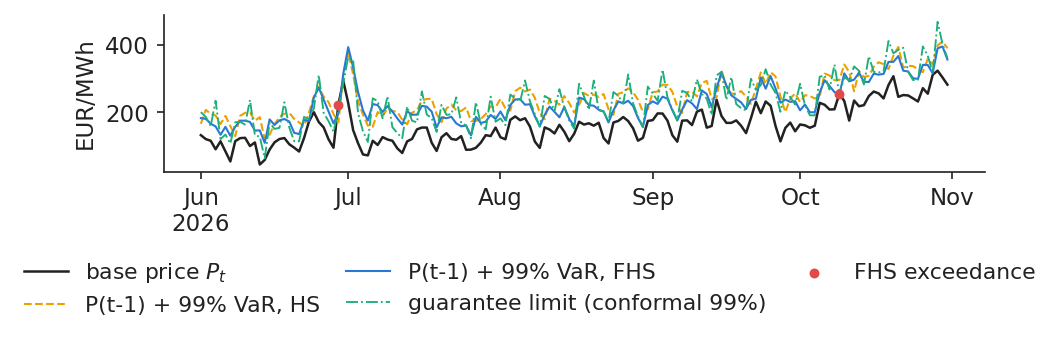
              Case study: in 2026 the price doubled gradually, without jumps

              Slide 44 in the PDF

              The monthly mean of the day-ahead price was 122.99 EUR/MWh in June 2026 and 239.32 in October, with a peak of 323.76 EUR/MWh on 29 Oct 2026. The rise came gradually, through many moderate daily changes rather than a few jumps. Over the 153 days of the period, a correct 99% VaR should have been exceeded 1.5 times; FHS was exceeded 2 times, HS once and the normal VaR 3 times. By the standard of the daily VaR, nothing alarming happened.

              In practice: a slow rise passes the VaR tests and still drains cash: watch the price level too.
              Chart: Case study: in 2026 the price doubled gradually, without jumps

              Romanian day-ahead base price and the 99% VaR forecasts, 1 Jun to 31 Oct 2026, with the exceedances marked.

              Source: energy-charts.info (Fraunhofer ISE); OPCOM day-ahead prices for Romania, via ENTSO-E; own estimates. Data: daily, 2026-06-01 to 2026-10-31.

              Case study: market risk and liquidity needs in 2026

              Slide 45 in the PDF

              Market risk barely moved. The FHS 99% VaR was 61.64 EUR/MWh in June and 67.50 in October, and the ES test since 2023 does not reject FHS (\(Z_2\) = −0.083). Cash needs, however, doubled. The day-ahead guarantee for 100 MW, computed from the widened 99% quantile, rose from 0.416 to 0.776 million EUR per day. Orders would have exceeded the guarantee limit on 3 days, and on 6 without the widening.

              The supplier's monthly bill for 100 MW rose by +25.1% in August (2.38 million EUR), +16.2% in September (1.86 million) and +34.0% in October (4.68 million). Each month stayed below the 99% limit of +50.5%, but three overruns came in a row, and their cost accumulates. The drivers were external: the TTF gas price rose from 44.94 to 86.81 EUR/MWh between June and October, Brent averaged 108.34 USD in October and the Germany–Luxembourg price 169.48 EUR/MWh.

              In practice: a risk report needs a liquidity line next to VaR: guarantees, margins and the cumulative monthly overrun.

              A risk desk checklist for energy prices

              Slide 46 in the PDF

              The lecture can be condensed into four steps for a risk desk.

              • Measure. Define the position and the sign of the loss, buyer or seller. Use only data known at gate closure. Report VaR and ES from two methods, one of them filtered (FHS or EVT).
              • Check. Run the Kupiec and Christoffersen tests and the traffic light on several years, including 2021–2022. Use \(Z_2\) for ES, and never rank models on a few tail days.
              • Decide. Set limits in EUR of VaR, converted daily to MW. Size guarantees and credit lines from calibrated high quantiles. Keep a cash buffer for the margin a crisis would demand.
              • Report. In EUR and in MW, by month, with the liquidity next to the market risk.
              In practice: Assignment 2 (Task 5) applies this checklist to the cash flow of your own role.

              Wrap-up

              The wrap-up tests the main ideas with five short questions, summarises the lecture and points to the research of our group and to further reading.

              Self-assessment questions

              Slide 47 in the PDF
              1. Your 99% one-day VaR for 100 MW is 162 thousand EUR. What does it promise, and what does it not say?
                Answer: on about 1 day in 100 the loss should exceed it. It says nothing about how large the loss is on those days, which is what ES (162 thousand EUR at 97.5%) measures.
              2. Over the last 250 days your 99% VaR was exceeded 7 times. What zone is it in, and what does Kupiec say?
                Answer: the yellow zone (5–9). The Kupiec test gives \(\text{LR}_{uc}\) = 5.50 and \(p\) = 0.019, so the model is rejected at 5%. Recalibrate it, for example by moving from HS to FHS, and keep watching.
              3. Your chief financial officer computes the 10-day VaR as \(\sqrt{10}\) times the 1-day VaR. Is that prudent or wasteful for power?
                Answer: wasteful. Power prices revert, and the empirical 10-day 99% quantile is only 1.72 times the 1-day one in Romania, not 3.16.
              4. You sold 100 lots of Brent to hedge your production, and today the price rises by 5 USD per barrel. What happens tonight?
                Answer: you pay a variation margin of 100 × 1,000 × 5 = 500,000 USD in cash. The physical oil you sell later is worth more, but the cash leaves today.
              5. Your 99% quantile forecast of tomorrow's price was exceeded on 111 days out of 3,585. What do you do?
                Answer: widen the tail with a conformal correction from recent errors. Coverage rises from 96.90% to 98.47% for 7.5% more guarantee.

              VaR is a quantile of tomorrow's loss and ES the mean of the loss beyond it. On power prices the normal curve fails, the filtered methods, FHS and EVT, come closest to their promise, and none was right in 2021–2022. The same quantiles set position limits, exchange margins and the day-ahead guarantee. The 2026 case study shows that liquidity, not VaR, is the first casualty of a price rise. The next lecture turns to hedging with derivatives (Lecture 5).

              Research from our group on energy risk

              Slide 53 in the PDF

              Three recent papers from our group, at the Bucharest University of Economic Studies and the Romanian Academy, Institute for Economic Forecasting, address the topics of this lecture. Their findings are those stated in the papers; the numbers on the other slides come from our own data.

              • Energy Financial Risk Meter (Toma, Dima, Grecu, Pele and Lessmann, 2026). The paper builds a systemic-risk indicator for the EU energy sector from LASSO quantile regressions on 100 companies; the indicator captures the 2020 and 2022 shocks (case study C4).
              • Foundation models for VaR and ES (Jheng, Tak, Găman, Mazurencu-Marinescu-Pele and Pele, 2026). The paper uses ten daily return series from five Central and Eastern European (CEE) markets, including Romania, out of sample in 2018–2025. It applies three pre-trained time-series models, without fine-tuning, against classical benchmarks, and evaluates them with the Kupiec, Christoffersen and Acerbi–Székely tests and the Basel traffic light. The best raw model has a green-zone rate of 90%, which rises to 96.7% after a rolling conformal calibration, the highest of all models.
              • How precise is an ES comparison? (Pele and Mazurencu-Marinescu-Pele, 2026). The paper turns the \((n\alpha)^{-1/2}\) precision limit of ES into four practical diagnostics, including a sample-size rule. On global financial assets it finds that about one in five pairwise ES comparisons cannot be trusted at regulatory tail levels.

              Further reading and resources

              Slide 54 in the PDF
              • McNeil, Frey and Embrechts, Quantitative Risk Management, 2nd edition: VaR, ES, EVT and backtesting.
              • Christoffersen, Elements of Financial Risk Management, 2nd edition: FHS and backtests, with exercises.
              • ECB, Financial stability risks from energy derivatives markets (2022): ecb.europa.eu.
              • This course: code, data and notebooks on github.com/danpele/EMQA; the notebook reproduces every chart and number of this lecture.
              • Assignment 2, Task 5: VaR and ES of your role's cash flow, with backtests.
              • OPCOM, the day-ahead guarantee procedure: opcom.ro.

              Appendix

              The appendix gives the derivations behind the ES formulas of the normal, Student-t and generalised Pareto curves, the backtests in full and the backtest table for Germany–Luxembourg.

              Appendix A: ES of the normal and Student-t distributions

              Slide 59 in the PDF

              For the normal curve, ES is the mean of the loss above the quantile:

              \[\text{ES}^{N}_\alpha=\frac{1}{1-\alpha}\int_{z_\alpha}^{\infty}(\mu+\sigma z)\varphi(z)\,dz=\mu+\sigma\frac{\varphi(z_\alpha)}{1-\alpha}\]
              (4.23)

              where \(z\) is the standard normal variable, \(\varphi\) its density, \(z_\alpha\) its \(\alpha\)-quantile and \(\mu\), \(\sigma\) the mean and standard deviation. The step uses \(\int_{c}^{\infty}z\varphi(z)\,dz=\varphi(c)\), because the derivative of \(\varphi\) is \(-z\varphi\). At \(\alpha\) = 0.975, ES\(^N\) = \(\mu\) + 2.338\(\sigma\), almost equal to VaR\(^N_{0.99}\) = \(\mu\) + 2.326\(\sigma\): this is why FRTB could swap one for the other.

              For the Student-t curve,

              \[\text{ES}^{t}_\alpha=m+s\,\frac{g_\nu(t_{\nu,\alpha})}{1-\alpha}\cdot\frac{\nu+t_{\nu,\alpha}^{2}}{\nu-1}, \quad \nu>1\]
              (4.24)

              where \(m\), \(s\) and \(\nu\) are the location, scale and degrees of freedom and \(t_{\nu,\alpha}\), \(g_\nu\) the quantile and density of the standard Student-t. It follows from \(\int_c^\infty x\,g_\nu(x)\,dx=g_\nu(c)\,(\nu+c^2)/(\nu-1)\). For \(\nu\le 1\) the mean, hence ES, does not exist. We fit \((m,s,\nu)\) by MLE every day and keep \(\nu\) at least 2.2 so that the variance exists (McNeil, Frey and Embrechts, 2015).

              Appendix B: VaR and ES from the generalised Pareto tail

              Slide 60 in the PDF

              By the Pickands–Balkema–de Haan theorem, for a high threshold \(u\) the excesses over \(u\) are approximately GPD for almost all distributions. The tail probability above \(u\) is then

              \[\Pr(Z>z)\approx\frac{N_u}{n}\Big(1+\xi\frac{z-u}{\beta}\Big)^{-1/\xi}, \quad z>u\]
              (4.25)

              where \(N_u/n\) is the share of the \(n\) observations above \(u\), \(\xi\) the shape and \(\beta\) the scale. Setting \(\Pr(Z>\text{VaR}_\alpha)=1-\alpha\) and solving gives

              \[\text{VaR}_\alpha=u+\frac{\beta}{\xi}\Big[\Big(\frac{n(1-\alpha)}{N_u}\Big)^{-\xi}-1\Big]\]
              (4.26)

              For the GPD the mean excess over a level \(v\) above \(u\) is linear in \(v\), provided \(\xi<1\):

              \[\E[Z-v\mid Z>v]=\frac{\beta+\xi(v-u)}{1-\xi} \quad\Rightarrow\quad \text{ES}_\alpha=\frac{\text{VaR}_\alpha+\beta-\xi u}{1-\xi}\]
              (4.27)

              The sign of \(\xi\) classifies the tail: \(\xi>0\) is a heavy tail, \(\xi=0\) an exponential tail and \(\xi<0\) a bounded tail. Conditional EVT applies these formulas to the standardised shocks \(z_t=e_t/\sigma_t\) and then sets VaR\(_t=\mu_{d(t)}+\sigma_t\,\)VaR\(^z_\alpha\), where VaR\(^z_\alpha\) is the GPD quantile of the shocks (McNeil and Frey, 2000).

              Appendix C: the three backtests in full

              Slide 61 in the PDF

              Kupiec and Christoffersen. Under \(H_0\) each \(I_t\) is an independent Bernoulli(\(p\)) variable, and \(\text{LR}_{uc}\) compares the promised share \(p\) with the observed \(\hat p\). \(\text{LR}_{ind}\) compares a first-order Markov chain with independence. The joint statistic \(\text{LR}_{cc}\) = \(\text{LR}_{uc}\) + \(\text{LR}_{ind}\) follows \(\chi^2_2\), with a 5% critical value of 5.99.

              Basel traffic light. For a correct model, the number of exceedances in 250 days is \(x\sim\) Binomial(250, 0.01). Then \(\Pr(x\le4)\) = 89.22%, \(\Pr(5\le x\le9)\) = 10.76% and \(\Pr(x\ge10)\) = 0.025% (BCBS, 1996).

              Acerbi–Székely test. When VaR and ES are correct, \(\E[L_tI_t]=(1-\alpha)\text{ES}_t\), so \(\E[Z_2]=0\). \(Z_2\) mixes a VaR error, a wrong count of \(I_t\), with an ES error, a wrong size of the tail losses; ES alone is not elicitable (Gneiting, 2011), so it is tested together with VaR. Our \(p\)-value comes from 2,000 simulated paths, each day drawn from that model's predictive distribution: the window for HS, \(\mu+\sigma z^*\) for FHS, where \(z^*\) is a resampled shock, and the GPD above \(u\) for EVT (Acerbi and Székely, 2014).

              Appendix D: the same backtest for Germany–Luxembourg

              Slide 62 in the PDF

              The backtest for the Germany–Luxembourg zone covers 1 Jan 2017 to 31 Oct 2026, 3,591 days, with the same methods and windows as for Romania.

              DE-LU95%: shareKupiec p99%: countshareKupiec pChr. pred, %Z2p
              HS6.38<0.001601.67<0.0010.9989.20.529<0.001
              Normal6.66<0.0011072.98<0.0010.33216.31.250<0.001
              Student-t8.33<0.001671.87<0.0010.1749.00.6170.001
              FHS5.820.028581.62<0.0010.9482.70.3050.009
              EVT5.930.013531.480.0070.8110.70.2830.007

              The ranking is the same as in Romania: the normal VaR is the worst and the filtered methods are the best.

              Abbreviations

              APCanti-procyclicality tools of a CCP
              AUCarea under the curve (0.5 = no skill, 1 = perfect)
              BCBSBasel Committee on Banking Supervision
              CARDIcarbon risk dynamic indicator
              CCPcentral counterparty (clearing house)
              CEECentral and Eastern Europe
              CETCentral European Time
              CFaRcash-flow-at-risk
              CISSComposite Indicator of Systemic Stress (ECB)
              DE-LUGermany–Luxembourg bidding zone
              ECBEuropean Central Bank
              EFRMEnergy Financial Risk Meter
              EMIREuropean Market Infrastructure Regulation (EU) No 648/2012
              ENTSO-EEuropean Network of Transmission System Operators for Electricity
              EPEXEPEX SPOT power exchange
              ESexpected shortfall
              EUEuropean Union
              EUReuro
              EVTextreme value theory
              FHSfiltered historical simulation
              FRMFinancial Risk Meter
              FRTBFundamental Review of the Trading Book (Basel market-risk rules)
              GARCHgeneralised autoregressive conditional heteroskedasticity
              GPDgeneralised Pareto distribution
              HShistorical simulation
              ICEIntercontinental Exchange (ICE Futures Europe)
              IMinitial margin
              ISEFraunhofer Institute for Solar Energy Systems
              LASSOleast absolute shrinkage and selection operator
              LRlikelihood ratio
              MLEmaximum likelihood estimation
              MWmegawatt
              MWhmegawatt-hour
              OPCOMRomanian electricity and gas market operator
              POTpeaks over threshold
              PZUPiața pentru Ziua Următoare (day-ahead market)
              QRquantile regression
              QRAquantile regression averaging (Lecture 2)
              RORomania (bidding zone)
              RTSregulatory technical standards
              TTFTitle Transfer Facility (Dutch gas hub)
              USDUnited States dollar
              VaRvalue-at-risk
              VMvariation margin

              References

              • Acerbi, C. & Székely, B. (2014). Backtesting expected shortfall. Risk, 27(11), 76–81. risk.net
              • Acerbi, C. & Tasche, D. (2002). On the coherence of expected shortfall. Journal of Banking & Finance, 26(7), 1487–1503. doi:10.1016/S0378-4266(02)00283-2
              • Artzner, P., Delbaen, F., Eber, J.-M. & Heath, D. (1999). Coherent measures of risk. Mathematical Finance, 9(3), 203–228. doi:10.1111/1467-9965.00068
              • Balkema, A. A. & de Haan, L. (1974). Residual life time at great age. Annals of Probability, 2(5), 792–804. doi:10.1214/aop/1176996548
              • Barone-Adesi, G., Giannopoulos, K. & Vosper, L. (1999). VaR without correlations for portfolios of derivative securities. Journal of Futures Markets, 19(5), 583–602. doi.org (Wiley)
              • BCBS (1996). Supervisory framework for the use of “backtesting” in conjunction with the internal models approach to market risk capital requirements. Basel Committee on Banking Supervision, January 1996. bis.org/publ/bcbs22.htm
              • BCBS (2019). Minimum capital requirements for market risk. Basel Committee on Banking Supervision, January 2019. bis.org/bcbs/publ/d457.htm
              • Bollerslev, T. (1986). Generalized autoregressive conditional heteroskedasticity. Journal of Econometrics, 31(3), 307–327. doi:10.1016/0304-4076(86)90063-1
              • Chan, K. F. & Gray, P. (2006). Using extreme value theory to measure value-at-risk for daily electricity spot prices. International Journal of Forecasting, 22(2), 283–300. doi:10.1016/j.ijforecast.2005.10.002
              • Christoffersen, P. F. (1998). Evaluating interval forecasts. International Economic Review, 39(4), 841–862. doi:10.2307/2527341
              • Christoffersen, P. F. (2012). Elements of Financial Risk Management, 2nd ed. Academic Press. elsevier.com
              • Commission Delegated Regulation (EU) No 153/2013 of 19 December 2012 on requirements for central counterparties (RTS under EMIR), Official Journal of the EU, L 52, 23.2.2013, Art. 24–28. eur-lex.europa.eu/eli/reg_del/2013/153/oj
              • Commission Delegated Regulation (EU) 2022/2311 of 21 October 2022 as regards temporary emergency measures on collateral requirements. Official Journal of the EU, L 307, 28.11.2022. eur-lex.europa.eu/eli/reg_del/2022/2311/oj
              • ECB — Furtuna, O., Grassi, A., Ianiro, A., Kallage, K., Koci, R., Lenoci, F., Sowiński, A. & Vacirca, F. (2022). Financial stability risks from energy derivatives markets. Financial Stability Review, European Central Bank, November 2022. ecb.europa.eu
              • Gneiting, T. (2011). Making and evaluating point forecasts. Journal of the American Statistical Association, 106(494), 746–762. doi:10.1198/jasa.2011.r10138
              • Jheng, S.-L., Tak, R., Găman, Ș., Mazurencu-Marinescu-Pele, M. & Pele, D. T. (2026). Can foundation models manage risk? Zero-shot VaR and ES forecasting with conformal calibration in CEE markets. Economic Computation and Economic Cybernetics Studies and Research, 60(2), 267–290. doi:10.24818/18423264/60.2.26.14
              • Jorion, P. (2007). Value at Risk: The New Benchmark for Managing Financial Risk, 3rd ed. McGraw-Hill. mheducation.com.au
              • Koenker, R. & Bassett, G. (1978). Regression quantiles. Econometrica, 46(1), 33–50. doi:10.2307/1913643
              • Kupiec, P. H. (1995). Techniques for verifying the accuracy of risk measurement models. Journal of Derivatives, 3(2), 73–84. doi:10.3905/jod.1995.407942
              • McNeil, A. J. & Frey, R. (2000). Estimation of tail-related risk measures for heteroscedastic financial time series: An extreme value approach. Journal of Empirical Finance, 7(3–4), 271–300. doi:10.1016/S0927-5398(00)00012-8
              • McNeil, A. J., Frey, R. & Embrechts, P. (2015). Quantitative Risk Management: Concepts, Techniques and Tools, revised ed. Princeton University Press. press.princeton.edu
              • Nowotarski, J. & Weron, R. (2018). Recent advances in electricity price forecasting: A review of probabilistic forecasting. Renewable and Sustainable Energy Reviews, 81, 1548–1568. doi:10.1016/j.rser.2017.05.234
              • OPCOM (2025). Procedura privind constituirea, verificarea și utilizarea garanțiilor financiare pentru participarea la Piața pentru Ziua Următoare, rev. 10, May 2025. opcom.ro
              • Pele, D. T. & Mazurencu-Marinescu-Pele, M. (2026). Finite-sample precision limits for expected shortfall forecast comparisons. Mathematics, 14(13), 2316. doi:10.3390/math14132316
              • Pele, D. T., Bolovăneanu, V., Ginavar, A. T., Lessmann, S. & Härdle, W. K. (2026). Recalibrating tail risk forecasts under temporal dependence: conformal audit of foundation models for VaR forecasting. AIDA Conference, Bucharest University of Economic Studies, 4 June 2026. github.com/danpele/EMQA/resources/aida2026
              • Pickands, J. (1975). Statistical inference using extreme order statistics. Annals of Statistics, 3(1), 119–131. doi:10.1214/aos/1176343003
              • Romano, Y., Patterson, E. & Candès, E. (2019). Conformalized quantile regression. Advances in Neural Information Processing Systems, 32, 3543–3553. proceedings.neurips.cc
              • Toma, F.-M., Dima, D.-M., Grecu, R., Pele, D. T. & Lessmann, S. (2026). Energy Financial Risk Meter: Systemic risk in the EU energy sector. SSRN Working Paper 6985301. doi:10.2139/ssrn.6985301
              • Toma, F.-M. (2026). Energy Financial Risk Meter: systemic risk in the EU energy sector (with D.-M. Dima, R. Grecu, D. T. Pele and S. Lessmann). AIDA Conference, Bucharest University of Economic Studies, 3 June 2026. github.com/danpele/EMQA/resources/aida2026
              • Wang, R., Härdle, W. K. & Zhang, L. (2025). Measuring carbon risk dynamics. SSRN Working Paper 5757742. doi:10.2139/ssrn.5757742
              • Wang, R., Härdle, W. K. & Zhang, L. (2026). Measuring carbon risk dynamics. AIDA Conference, Bucharest University of Economic Studies, 5 June 2026. github.com/danpele/EMQA/resources/aida2026
              • Weron, R. (2014). Electricity price forecasting: A review of the state-of-the-art with a look into the future. International Journal of Forecasting, 30(4), 1030–1081. doi:10.1016/j.ijforecast.2014.08.008

              Text written for the web version of the lecture; numbers, charts and sources come from the slides and their Quantlets.