

The slide of the lecture is on the left, the same figure on the right, computed in the browser from the same data. The ▶ button moves the parameter step by step.
Value-at-Risk and Expected Shortfall · Coherent Risk Measures · Estimation Methods · How Precise Are VaR and ES? · Conditional VaR and ES · Extreme Value Theory · The Horizon: Square-Root-of-Time · Portfolio VaR and Risk Contributions · Liquidity and Regulation · Case Studies: Deep Quantile Regression and Time-Varying Tail Shape · AI for Scientific Discovery
Value-at-Risk and Expected Shortfall
VaR and ES on the S&P 500
Answer
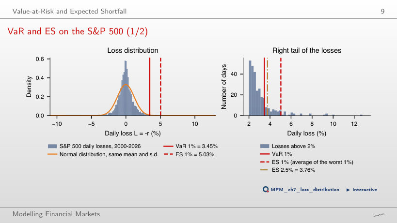
VaR stays at 3.45%, and ES rises from 5.03% to about 5.18%. The ten modified losses lie above the observations that determine the quantile, so VaR does not change. ES 1% averages the largest nα = 67.17 losses (the last one with weight 0.17); all ten enter with weight 1, so ES rises by 10/67.17 ≈ 0.15 pp. VaR locates the threshold; ES also accounts for the severity of the losses beyond it. The Normal distribution with the same mean and standard deviation gives a VaR 1% of 2.80% and an ES 1% of 3.21%.
Coherent Risk Measures
Subadditivity of VaR and ES: a Counterexample
Answer
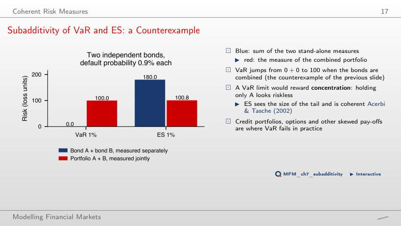
100. The probability that at least one defaults becomes 2.19%, above 1%, but the probability of two defaults is only 0.012%, below 1%; the portfolio VaR 1% stays at 100. Each individual VaR becomes 100, so their sum is 200 ≥ 100 and subadditivity holds: 200 is the sum of the individual VaRs, not the portfolio VaR, and 0 was the individual VaR at 0.9%. At 0.9% (the slide), the probability of at least one default is 1.79%, and the portfolio VaR, 100, exceeds the sum 0 + 0. In this example, VaR violates subadditivity only when the default probability lies between about 0.5% and 1%. ES is subadditive: at 0.9%, 100.8 for the portfolio against 90 + 90 = 180.
Estimation Methods
Five Methods Across Tail Probabilities
Answer
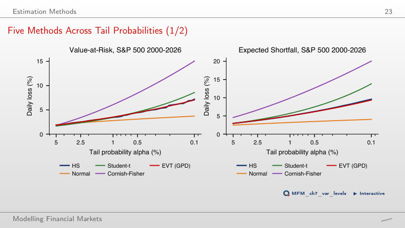
At α = 0.1%: the gap is 11.34 pp (Cornish–Fisher 15.06% minus the Normal distribution 3.72%), against 0.30 pp at α = 5%, where all five values lie between 1.67% and 1.97%. At α = 0.1%, VaR is 7.22% historical, 7.04% with EVT and 8.58% with Student-t. Where data are scarce, the tail assumptions drive the estimate: the same statistical target does not force different models to give close values.
How Precise Are VaR and ES?
Precision on the S&P 500
Answer
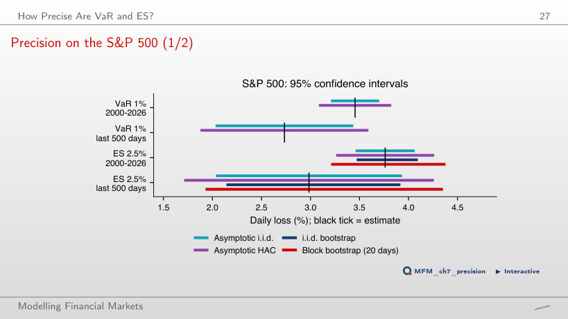
The tail mass is 500 × 0.025 = 12.5 observations: sum the 12 largest losses and 0.5 of the 13th, then divide by 12.5. With 13 equal weights, the effective tail level becomes 13/500 = 2.6%. The 95% HAC interval of this ES is 2.55 pp wide and the block bootstrap interval 2.42 pp. On the 2000–2026 sample, volatility clustering widens the ES interval from 0.60 pp (i.i.d.) to 1.00 pp (HAC), and the bootstrap interval from 0.62 pp to 1.17 pp.
Conditional VaR and ES
Historical vs Filtered Historical Simulation: S&P 500
Answer
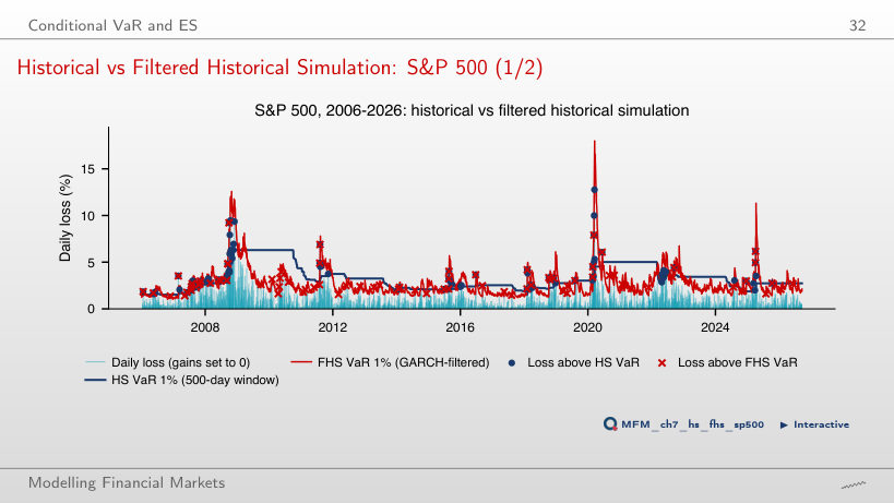
FHS comes closest to the 1% target: 80 of 5,210 days, that is 1.54%, against 1.67% for historical simulation on 500 days and 2.34% for GARCH with Normal shocks. The historical window updates daily, but gives equal weight to observations from different volatility regimes and may adapt slowly; its exceedances come in clusters, in 2008 and 2020. Closeness to a 1% exceedance rate does not by itself establish independence of the exceedances.
CAViaR vs Filtered Historical Simulation, Out of Sample
Answer
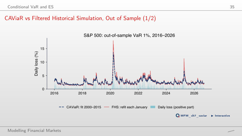
About 6.4 days: the half-life is ln 0.5 / ln β₁, with β₁ = 0.897. Out of sample, in 2016–2026, CAViaR and FHS each have 35 exceedances (1.30%), and the mean pinball loss is 0.039 for CAViaR and 0.037 for FHS.
Extreme Value Theory
Monthly Maxima of S&P 500 Losses
Answer
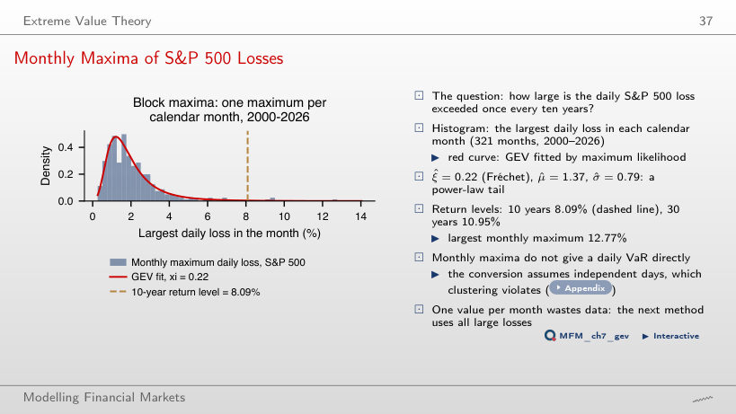
1/120 ≈ 0.83%. The blocks are months, so ten years contain 120 blocks; the return level 8.09% (ξ = 0.22) satisfies P(monthly maximum > 8.09%) = 1/120 in the fitted model. 1/10 confuses years with blocks; 1/2,520 treats days (252 per year) as blocks. The level does not mean that exceedances occur periodically, and an exceeding month may contain several days above the threshold. Four of the 321 monthly maxima exceed it; the largest observed monthly maximum is 12.77%.
Mean Excess Plot: S&P 500
Answer
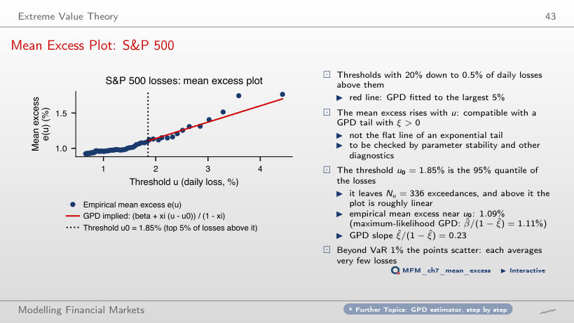
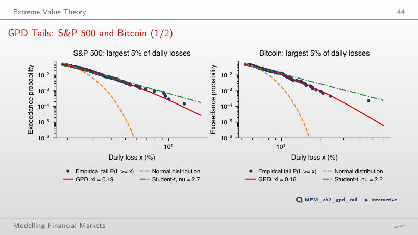
It is compatible with a GPD tail with 0 < ξ < 1: the mean excess is then finite and linear in the threshold, with slope ξ/(1 − ξ) > 0; for ξ ≥ 1 the theoretical mean excess is infinite. The current estimate gives ξ = 0.19 and slope 0.23. At the threshold u₀ = 1.85% (the largest 5% of losses, 336 exceedances), the empirical mean excess is 1.09% and the GPD gives 1.11%. The plot supports this approximation but does not prove it; threshold selection also requires checking parameter stability. For an exponential tail the plot would be flat.
GPD Tails: S&P 500 and Bitcoin
Answer
No: VaR depends on the threshold, the scale and the shape. The shape estimates are ξ = 0.16 (SE 0.078) for Bitcoin and ξ = 0.19 (SE 0.065) for the S&P 500; the large VaR gap comes from Bitcoin’s much larger scale. The individual standard errors assume independent exceedances, and the page does not compute a test of the difference between the two ξ; nor do close estimates prove equal shapes. An inferential conclusion requires the uncertainty of the difference, accounting for dependence in the data.
Conditional EVT on the S&P 500
Answer
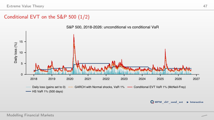
The tail model of the standardised losses. Conditional EVT keeps the GARCH filter and the level α, but replaces the Normal tail of the standardised shocks with a GPD approximation. In 2018–2026 (2,190 days, 21.9 exceedances expected), the exceedance rate of VaR 1% falls from 2.42% (53 days) with GARCH-Normal to 1.23% (27) with conditional EVT; historical simulation on 500 days has 1.60% (35). This comparison alone does not establish that the whole specification is correct.
The Horizon: Square-Root-of-Time
Square-Root-of-Time in the Data
Answer
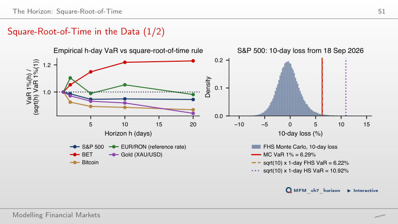
No. Without autocorrelation and with constant variance, the h-day variance is h times the daily one, but the quantile of the sum also depends on the shape of its distribution, which changes with h (fat tails, volatility clustering). The rule is exact, for example, for i.i.d. Normal losses with zero mean. In the data, the ratio at h = 10 is 1.22 for the BET (first-order autocorrelation 0.109) and 1.05 for EUR/RON, so the rule understates the risk; for the S&P 500 (0.95), gold (0.92) and Bitcoin (0.89) the rule is conservative. For the S&P 500, filtered Monte Carlo gives 6.29%, against 6.22% for √10 × the one-day filtered VaR.
Portfolio VaR and Risk Contributions
Who Contributes the Risk?
Answer
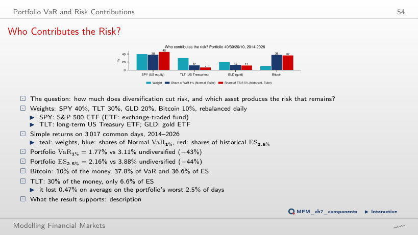
It rises from 36.6% to 87.0%: the capital weight triples, the ES share grows 2.4 times. The Euler contribution to ES is the weight times Bitcoin’s average loss on the portfolio’s tail days, and those days change with the weight; the risk share is not the capital share and does not grow in proportion to it. At the slide’s weight, 10%, Bitcoin accounts for 37.8% of VaR 1% (Normal, Euler) and 36.6% of ES 2.5% (historical); TLT, with 30% of the capital, accounts for only 6.6% of ES. Diversification lowers VaR 1% from 3.11% (the sum of the individual VaRs) to 1.77%.
Liquidity and Regulation
VaR 1% vs ES 2.5% on Five Assets
Answer
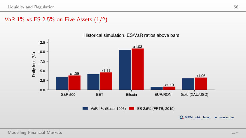
They fall below 1: at ES 5%, the ratios lie between 0.81 (Bitcoin) and 0.86 (S&P 500), and under the Normal distribution with zero mean the ratio is 0.887. ES ≥ VaR holds only at the same level α; ES 5% averages over the worst 5% of days, a less extreme tail than that of VaR 1%. At the Basel level, ES 2.5%, the ratios lie between 1.03 (Bitcoin) and 1.11 (BET): 1.09 for the S&P 500, 1.10 for EUR/RON and 1.06 for gold. The zero-mean Normal benchmark is φ(z₀.₉₇₅)/(0.025 × z₀.₉₉) = 2.338/2.326 ≈ 1.005; with a nonzero mean, the mean enters both ES and VaR and the ratio changes.
Case Studies: Deep Quantile Regression and Time-Varying Tail Shape
Case Study: Relative Forecast Error, α = 1%
Answer
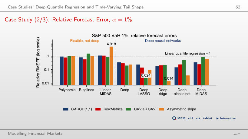
Not directly. All 20 bars of the deep networks (deep MIDAS included) are below 1, between 0.014 and 0.850, but RMSFE is minimised by the conditional mean, not by the quantile. The accuracy of a quantile forecast is compared with the pinball loss. The result also comes from a single fixed calibration window.
Second Case Study (2/4): Tail Shape and Scale of the S&P 500, 2000–2026
Answer
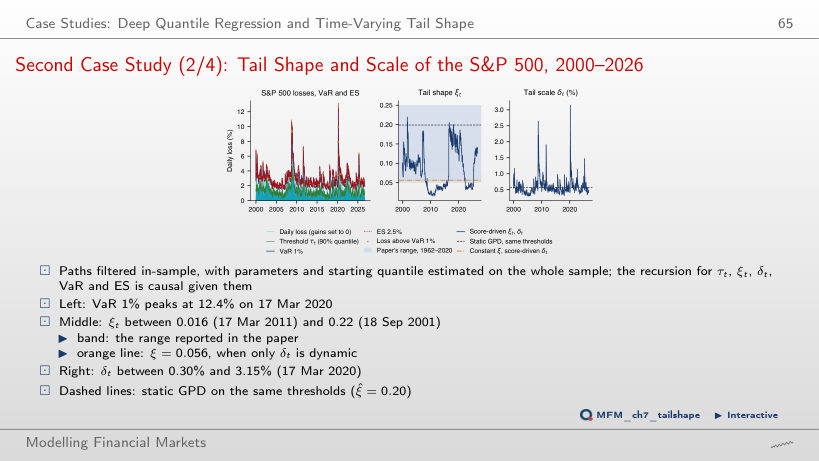
It rises by about 1.92: ΔAIC = 2 × 2 − 2 × 1.04 = 1.92, so AIC penalises the model with dynamic ξt (774 against 772). −2.08 ignores the parameter penalty; 2.96 omits the factor 2 on the log-likelihood term. The log-likelihood is −380.85 with dynamic ξt and δt, against −381.89 with constant ξ (0.056) and dynamic δt. The static GPD has AIC 853, so the fall 853 → 774 comes from the dynamics of the scale δt. With aξ = 0, ξt stays fixed at 0.083. The filtered VaR 1% is exceeded on 61 of 6,717 days (0.91%).
AI for Scientific Discovery
Mini-Case: Can We Rank ES Models?
Answer
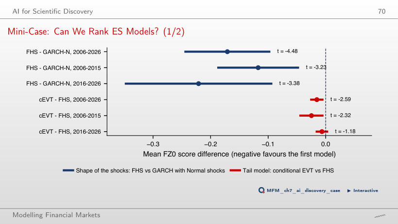
It establishes neither an EVT advantage nor equivalence. The interval contains zero and differences of both signs (t = −1.18), so the advantage of conditional EVT is not significant in 2016–2026. The pre-registered rule requires t < −1.96 (two-sided test at 5%) in both subperiods; in 2006–2015, t = −2.32, and over 2006–2026, t = −2.59. Equivalence would require a margin fixed in advance and a dedicated analysis. FHS against GARCH–Normal meets the rule: t = −3.23 and t = −3.38.
Daily losses L = −r, in %, up to 18 September 2026. S&P 500, BET, Bitcoin, gold (XAU/USD) and the ETFs SPY, TLT, GLD: EODHD daily prices; EUR/RON: the NBR reference rate. Case studies: Table 6 of Chronopoulos, Raftapostolos and Kapetanios (2024), Journal of Financial Econometrics; the score-driven GPD model of D’Innocenzo, Lucas, Schwaab and Zhang (2024), Journal of Business & Economic Statistics, estimated on the course data.