Bucharest University of Economic Studies IDA Institute Digital Assets Blockchain Research Center AI4EFin Artificial Intelligence for Energy Finance Romanian Academy, Institute for Economic Forecasting MSCA Digital Finance
Can We Trade the Sentiment That Models Read in the News?
“I find that high media pessimism predicts downward pressure on market prices followed by a reversion to fundamentals, and unusually high or low pessimism predicts high market trading volume.” — Tetlock (2007)
The chapter compares dictionaries, FinBERT, zero-shot LLMs (large language models) and embeddings on the same labelled texts
on Twitter, the best is the simplest supervised model, TF-IDF (weighted word frequencies) + logistic regression: 83.2% accuracy, against 74.2% for Qwen2.5-7B and 72.5% for FinBERT
On 16 large US (United States) stocks with 106 820 news headlines, the score explains the same-day price move
FinBERT: +39.2 bp per standard deviation of the score (\(t\) = +17.27); bp: basis points, 1 bp = 0.01%
A daily long-short strategy on the sign of the score brings no net profit
Qwen2.5-7B: +5.64 bp per day before costs, \(p\) = 0.071 after the Holm correction
the break-even cost, 1.5 bp per trade, is below the assumed cost of 5 bp
LLMs remember market history
asked only for the month, Qwen2.5-14B separates up from down months of the S&P 500 (Standard & Poor's) with an AUC (Area Under the, ROC Curve) of 0.69 (area under the ROC curve; 0.5 = no discrimination)
I find that high media pessimism predicts downward pressure on market prices followed by a reversion to fundamentals, and unusually high or low pessimism predicts high market trading volume.
Tetlock (2007) measures the pessimism of a Wall Street Journal column and shows that it is followed by downward pressure on prices and then by a reversion. The chapter starts from the same question with today's tools: how well do models read the sentiment of a financial text, and can that sentiment be traded? Four routes are compared: word dictionaries, the FinBERT model trained on labelled financial sentences, large language models (LLMs) used zero-shot, and embeddings followed by a classifier. General dictionaries misread financial text: in the lists used here, 77% of the negative words of the Harvard General Inquirer (GI) are not among the negative words of the financial dictionary of Loughran & McDonald (2011).
On financial headlines from Twitter, no model wins outright. The best is the simplest supervised model, TF-IDF (term frequency–inverse document frequency) followed by a logistic regression, with 83.2% accuracy, against 74.2% for Qwen2.5-7B and 72.5% for FinBERT. Labels from the target domain matter more than model size. An LLM also raises a look-ahead bias problem: asked only for the month, Qwen2.5-14B separates up from down months of the S&P 500 (Standard & Poor's) with an area under the ROC (Receiver Operating Characteristic, curve) curve (AUC) of 0.69, where 0.5 means no discrimination.
On 16 large US (United States) stocks, with 106 820 distinct headlines from FNSPID (Financial News and Stock Price Integration Dataset), the scores explain the price move on the day of the news: for FinBERT, one standard deviation of the score corresponds to an excess return 39.2 basis points (bp) higher. Many headlines, however, report the price move itself. A daily long-short strategy on the sign of the score, with positions opened after the news day, brings no net profit. The best score, Qwen2.5-7B, earns 5.64 bp per day before costs, but \(p\) = 0.071 after the Holm correction, and its break-even cost, 1.5 bp per trade, is below the assumed cost of 5 bp. The Sharpe ratio is +0.63 before costs and −1.48 after costs.
Sum of the daily excess returns of the long-short strategy (%), for the FinBERT, Qwen2.5-7B and LM (Loughran-McDonald, financial sentiment dictionary) scores, before costs and with 5 bp per trade. Interactive chart: “Cumulative Strategy Returns: No Net Profit” →
What you will be able to do
Compute the sentiment of a text with a dictionary, with FinBERT and with a zero-shot LLM.
Interpret a paired test for two classifiers evaluated on the same texts.
Interpret the overlap and memorisation tests of an LLM backtest.
Interpret the test of a sentiment signal, with correct timing, inference with few clusters, costs and a correction for multiple testing.
Derive the attenuation of the slope on a generated regressor.
Interpret prediction-powered inference intervals.
The Further Topics and the Appendix are reading for familiarisation.
Prices respond to information, and most of the information that reaches a market arrives as text: news, company filings, earnings calls, analyst reports, central-bank statements and social media. The chapter treats the tone of such text as a quantity to be measured, compares the instruments that measure it on the same labelled data, and then asks whether the measured tone of dated headlines can be traded once timing, costs and multiple testing are taken into account.
The first section fixes the vocabulary: what "text as data" means, which notion of sentiment is used, what the early literature found, and which four families of methods turn a document into a sentiment score.
Can Models Read News Sentiment, and Can We Trade It?
Information that moves prices reaches investors through many channels, and almost all of them are textual: news wires and newspapers, the periodic filings of listed companies, the transcripts of earnings calls, analyst reports, central-bank statements and, more recently, posts on social media. A model of how prices respond to news therefore needs, at some stage, a way of reading text.
Financial newspapers are as old as organised markets. The Wall Street Journal published its first issue on 8 July 1889, and the photograph on the slide shows that first page. The difference today is one of scale: millions of documents appear every day, far more than any analyst can read. Reading at this scale has to be delegated to an algorithm, and the quality of that algorithm becomes a measurement problem in its own right.
In brief
Prices move when information arrives, and most information arrives as text
News, company filings, earnings calls, analyst reports, central-bank statements, social media
Financial newspapers are as old as organised markets
The Wall Street Journal: first issue on 8 July 1889
Today: millions of documents per day, far more than any analyst can read
Gentzkow, Kelly & Taddy (2019) describe the general recipe of text as data in economics. A document \(d\) is first mapped to a numerical representation \(x_d\): word counts, scores or vectors. This representation is then mapped to a quantity of interest, such as sentiment, topic or risk, and that quantity enters an ordinary statistical model of an economic outcome, such as returns or volatility. Every step involves choices, and every choice can introduce error.
In this chapter the sentiment of a text is a property of the text: whether it is good, bad or neutral news for the asset it mentions. It is reported either as one of three classes or as a net score
where the two probabilities are those a classifier assigns to the positive and negative classes. This notion is distinct from investor sentiment, the mood of investors measured from market data (Baker & Wurgler, 2006). The surveys of Kearney & Liu (2014) and Loughran & McDonald (2016) cover both strands of the finance literature.
The chapter treats the score (15.1) as an estimate of the true tone of a text, measured with error. This view runs through all the sections: it determines how classifiers are evaluated against human labels, how regression slopes on scores are read, and how confidence intervals are built when model scores replace human labels.
Four contributions frame the empirical question. Antweiler & Frank (2004) study internet message-board posts about stocks and find that they help predict volatility, while their effect on returns is small. Tetlock (2007) measures pessimism in a Wall Street Journal column and finds that high media pessimism predicts downward pressure on prices, followed by a reversal; unusually high or low pessimism also predicts high trading volume.
Tetlock, Saar-Tsechansky & Macskassy (2008) move from the market to individual firms. Their measure is the share of negative words in firm-specific news, and it predicts lower earnings and lower returns. Prices incorporate this information only gradually, which is the kind of slow adjustment a trading strategy could exploit.
Shiller (2017) gives the broader motivation: popular stories spread like epidemics and influence economic decisions, and they can be measured through text. Shiller received the Nobel Prize in Economics in 2013, together with Fama and Hansen. Narratives can push prices away from fundamentals, a theme treated in Chapter 2 on market efficiency and Chapter 17 on bubbles and crashes.
The methods compared in the chapter fall into four families, which differ in how much labelled data they need. A dictionary counts the words of a document that appear on predefined positive and negative lists; it needs no labels. Three dictionaries are used:
the Harvard General Inquirer (GI), a general-purpose word list;
the Loughran–McDonald (LM) financial dictionary;
VADER (Valence Aware Dictionary and sEntiment Reasoner), a dictionary with rules built for social media.
A fine-tuned model such as FinBERT is a neural network trained on thousands of labelled sentences. A large language model (LLM), such as Qwen2.5 or the GPT (Generative Pre-trained Transformer) models of OpenAI, receives an instruction in plain language, the prompt, and classifies without any labelled example; this is zero-shot use. Finally, embeddings followed by a classifier turn each text into a generic vector, here from the MiniLM model, and fit a regression on hundreds to thousands of labels.
All four are compared on the same labelled data, with 95% confidence intervals (CI), and then tested on daily stock returns. A fifth route, text regressions with statistical theory (Taddy, 2013; Ke, Kelly & Xiu, 2019), is not tested in the body of the chapter; it is described in the Appendix.
In brief
Method
How it works
Labels needed
Examples
Dictionary
count listed words
none
GI, LM, VADER
Fine-tuned model
network trained on labelled sentences
thousands
FinBERT
Large language model
instruction in plain language (prompt)
none (zero-shot)
Qwen2.5, GPT
Embeddings + classifier
text vectors into a regression
hundreds to thousands
MiniLM
GI: the Harvard General Inquirer, a general-purpose word list; LM (Loughran-McDonald, financial sentiment dictionary): the Loughran–McDonald financial dictionary; VADER: Valence Aware Dictionary and sEntiment Reasoner, a dictionary with rules built for social media; GPT: Generative Pre-trained Transformer, the language models from OpenAI
We compare all four on the same labelled data, with 95% confidence intervals (CI)
Then we test whether any of them makes money on daily stock returns
A fifth route, text regressions with statistical theory, is not tested here (Appendix)
Taddy; Ke, Kelly and Xiu
Section summary
Text enters finance as data: a document is mapped to numbers, the numbers to a sentiment score, and the score to a model of returns. The early literature found that the tone of news is related to prices, volume and earnings, with slow adjustment. The four families of methods differ mainly in the amount of labelled data they need, and the following sections compare them on the same texts.
Dictionaries
The oldest method in finance measures tone by counting words from predefined lists. Its appeal is transparency: every score can be traced to the words that produced it. Its weakness is that a word list ignores context, and that a list built for one domain can misread another.
Can a Word List Measure the Tone of a Financial Text?
A dictionary method rests on the bag-of-words representation: a document is reduced to the counts of its words, and their order is ignored. Tokens are case-insensitive words, without digits and punctuation. A dictionary supplies a set \(\mathcal{P}\) of positive words and a set \(\mathcal{N}\) of negative words; let \(P_d\) and \(N_d\) be the numbers of positive and negative words in document \(d\).
with \(\tau_d = 0\) if \(P_d + N_d = 0\), and the predicted class is the sign of \(\tau_d\), neutral when \(\tau_d = 0\). A document with only positive listed words has tone \(+1\), one with only negative words has tone \(-1\), and a document with no listed word is neutral by construction.
The method is transparent, fast and needs no training data. Its limitation follows directly from (15.2): the sign of each word is fixed in advance, so the method is blind to context and to negation. "Not good" counts as positive, and a word whose meaning depends on its neighbours receives the same sign in every sentence.
In brief
Bag of words: a document is reduced to its word counts
Word order is ignored
Tokens: case-insensitive words, without digits and punctuation
A dictionary lists positive words \(\mathcal{P}\) and negative words \(\mathcal{N}\)
\(P_d\), \(N_d\): number of positive and negative words in document \(d\)
Tone: \(\tau_d = \dfrac{P_d - N_d}{P_d + N_d} \in [-1, 1]\), and \(\tau_d = 0\) if \(P_d + N_d = 0\); the class is the sign of \(\tau_d\) (neutral for \(\tau_d = 0\))
The Harvard General Inquirer (GI), word list Harvard IV-4, is a psychology dictionary from the 1960s, with 2,007 negative and 1,637 positive words. Loughran & McDonald (2011) built the LM dictionary from the annual reports (10-K filings) of US firms. It has 2,355 negative words and only 354 positive words. Their finding was that almost three quarters of the GI negative words are not negative in a financial context. In the lists used in this chapter, 1,552 GI negative words, 77% of them, are not LM negative words.
VADER (Hutto & Gilbert, 2014) contains about 7,500 terms with intensity scores and was built for social media. It adds rules for negation ("not good"), intensifiers ("very"), capital letters, exclamation marks and emoticons, and it returns a compound score in \([-1, 1]\), usually cut at \(\pm 0.05\) to obtain three classes.
The three dictionaries thus differ along two axes: the vocabulary (generic for GI and VADER, financial for LM) and the treatment of context (none for GI and LM, simple rules for VADER). The rules of VADER fix some context problems, but its vocabulary remains generic, like that of GI.
In brief
Harvard General Inquirer (GI), word list Harvard IV-4: a psychology dictionary from the 1960s
The chart examines the words on which GI and LM disagree, using the sentences of Financial PhraseBank, a corpus of news sentences labelled by human annotators and described in the next section. Each horizontal bar is a word; its length is the number of PhraseBank sentences that contain the word, and its colours split those sentences by the label the annotators gave them: positive, neutral or negative.
In the interactive version, the selector chooses the word list: words negative in GI but not in LM, or the reverse. The slider sets how many words are shown, and the ▶ button adds words one at a time. The readout below the chart counts the sentences and the share of them not labelled negative.
Question for the room "Service", "capital" and "board" are negative words in the Harvard IV-4 dictionary. In Financial PhraseBank, what proportion of the sentences containing each of these words is labelled negative?
Answer
Below 10% for each word: 2 of the 106 sentences with "service" (1.9%), 7 of the 104 with "capital" (6.7%) and 3 of the 79 with "board" (3.8%). The sign of a word in the dictionary does not determine the label of the sentence. Nor would a word unrelated to tone give 50%: it would occur in negative sentences at the frequency of the negative class in the corpus, 12.5%.
For the default list, the most frequent words, "service" (106 sentences), "capital" (104) and "board" (79), are business nouns. Only 2 of the 106 sentences with "service" (1.9%), 7 of the 104 with "capital" (6.7%) and 3 of the 79 with "board" (3.8%) are labelled negative. A word unrelated to tone would occur in negative sentences at the frequency of the negative class in the corpus, 12.5%; these words fall below even that.
The words that GI marks as negative and LM does not are, for the most part, ordinary vocabulary of business. "Service", "capital" and "board" appear in sentences that are not labelled negative in 98%, 93% and 96% of cases, and "vice", as in "vice president", in 100% of cases. Counting them as negative adds noise to the tone of every financial text that mentions them.
"Lower" is a different case: only 26% of its sentences are not labelled negative, so it is often a genuinely negative word. Yet "lower costs" is good news for a firm. The sign of "lower" depends on the next word, which no word list sees; this is the context problem of (15.2) in its purest form.
Taken together, the 964 PhraseBank sentences whose only GI-negative words are missing from the LM negative list are not labelled negative in 89% of cases. A worked example of one sentence scored by both dictionaries is in Further Topics.
In brief
Words negative in GI but not in LM
Ranked by the number of Financial PhraseBank sentences that contain them
Colour: the label human annotators gave the sentence
“Service” (106 sentences), “capital” (104) and “board” (79) are business nouns, not bad news
Not labelled negative: 98%, 93%, 96% of their sentences; “vice” (“vice president”): 100%
“Lower”: only 26% not negative, but “lower costs” is good news
The sign depends on the next word, which no word list sees
Of the 964 sentences whose only GI-negative words are missing from the LM negative list:
Dictionary tone (15.2) is transparent and cheap, but its quality depends on the list. A generic psychology dictionary counts business nouns as negative: in the lists used here, 77% of the GI negative words are not negative in LM, and sentences scored negative only by such words are not labelled negative in 89% of cases. No list sees context, so words such as "lower" keep the wrong sign whenever the next word reverses it.
Labelled Data and Evaluation
A classifier is judged by its agreement with human labels on texts it has not been trained on. This section describes the two labelled corpora, the metrics used when one class dominates, the paired test that compares two classifiers on the same texts, and the comparison of eleven classifiers.
Which Texts Do We Judge a Classifier On? Two Labelled Corpora
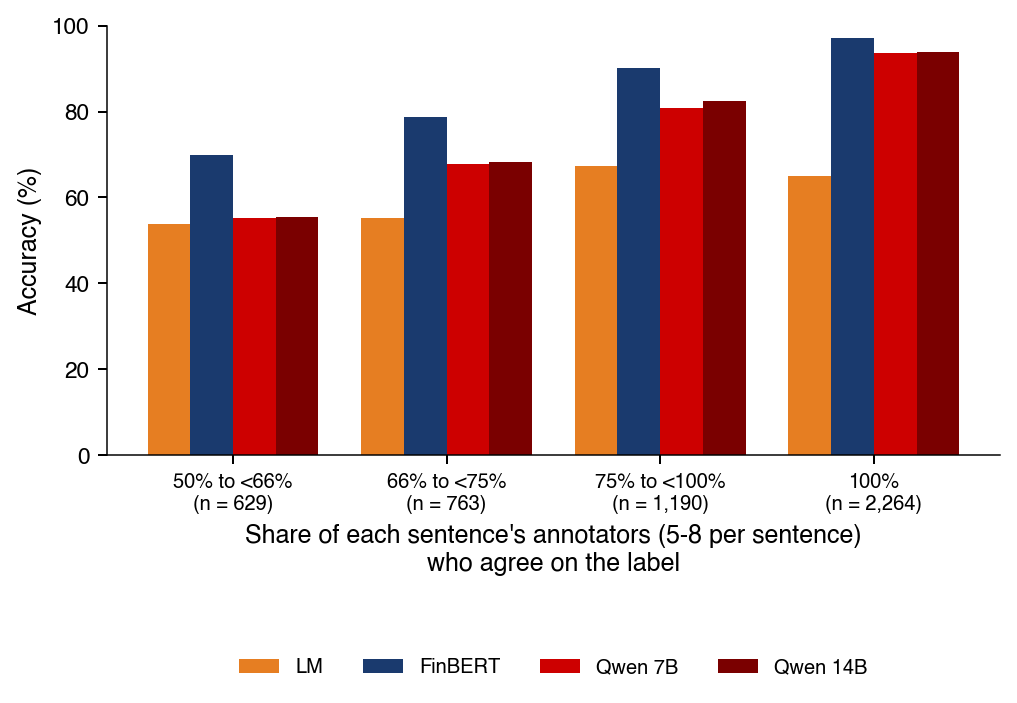
Financial PhraseBank (Malo et al., 2014) contains 4,846 sentences from financial news. They were labelled by a pool of 16 annotators with a finance background, 5 to 8 per sentence, who answered one question: is the sentence good, bad or neutral news for the investor? The corpus is released with agreement levels, the share of a sentence's annotators that chose the majority label: at least 50%, 66%, 75% or 100%. Full agreement is reached on 2,264 sentences, and 629 sentences have agreement below 66%. The labels are 59% neutral, 28% positive and 12% negative.
The second corpus, Twitter Financial News, is distributed on the Hugging Face Hub under the MIT (Massachusetts Institute of Technology) licence and contains financial headlines from 2022, labelled bearish, bullish or neutral. It has a training set of 9,543 headlines and a validation set of 2,388 headlines, which serves for evaluation throughout the chapter. Its labels are 66% neutral, 20% positive and 15% negative. The texts are short and noisy, with tickers and links, and are closer to the real news flow than the edited sentences of PhraseBank.
Two corpora are used because a result obtained on one need not carry over to the other. The comparison matters in particular for FinBERT, whose public version was fine-tuned on PhraseBank, as the section on language models shows.
Accuracy is the share of texts classified correctly, \(\text{acc} = \frac{1}{n}\sum_{i=1}^{n}\mathbf{1}\{\hat y_i = y_i\}\). When one class dominates, accuracy rewards a classifier that predicts that class most of the time. A metric that weighs the classes equally is needed to see whether the rare classes, here positive and negative news, are recognised at all.
For class \(k\), let \(TP_k\) be the number of texts of class \(k\) predicted as \(k\),\(FP_k\) the number of texts of other classes predicted as \(k\), and \(FN_k\) the number of texts of class \(k\) predicted as another class. Precision, recall and their harmonic mean are
with \(K = 3\) classes. Macro-F1 gives every class the same weight, however rare; the same metrics are used in Chapter 13.
The benchmark that always answers "neutral" shows the difference between the two metrics. On the Twitter validation set it reaches 66% accuracy, the share of neutral headlines. Its neutral recall is 1 and its neutral precision 0.656, so \(F1_{\text{neutral}} = 2 \times 0.656 \times 1/(0.656 + 1)\), that is 0.792, while \(F1 = 0\) for the two other classes. Its macro-F1 is therefore \(0.792/3\), only 26.4%.
In brief
The question: how do we compare classifiers when one class dominates?
When two classifiers A and B are evaluated on the same \(n\) texts, their accuracies are correlated: both find the easy texts easy and the hard texts hard. Two separate confidence intervals therefore do not answer whether one classifier is better. The comparison has to use the pairing.
Let \(n_{01}\) be the number of texts on which A is wrong and B is right, and \(n_{10}\) the number on which A is right and B is wrong. Texts on which the two classifiers agree, both right or both wrong, carry no information about the difference: the accuracy gap is \((n_{01} - n_{10})/n\). Under the null hypothesis of equal accuracy, each discordant text is equally likely to favour either classifier, so \(n_{01} \sim \text{Binomial}(n_{01} + n_{10}, 0.5)\), which gives an exact test. For large \(n_{01} + n_{10}\) the statistic
is approximately \(\chi^2_1\); the \(-1\) is a continuity correction.
A small example shows the exact version. If A is wrong and B right on 4 texts and the reverse happens on 1, then with \(X \sim \text{Binomial}(5, 0.5)\) the two-sided p-value is \(p = 2\,P(X \ge 4) = 2 \times 6/32 = 0.375\). Five discordant texts are far too few to separate the two classifiers. A worked example on real data, FinBERT against LM, is in the Appendix.
In brief
Two classifiers A and B on the same \(n\) texts: their accuracies are correlated
So two separate CIs do not answer the question
\(n_{01}\): number of texts where A is wrong and B is right
\(n_{10}\): number of texts where A is right and B is wrong
Texts on which both classifiers agree carry no information
The accuracy gap is \((n_{01} - n_{10})/n\)
Under \(H_0\) (equal accuracy), \(n_{01} \sim \text{Binomial}(n_{01} + n_{10}, 0.5)\)
The chart compares eleven classifiers on the two corpora. Each row is a method: the three dictionaries (GI, VADER, LM), two supervised models trained on Twitter labels, TF-IDF + LR (Logistic Regression) and MiniLM + LR, FinBERT and five zero-shot Qwen2.5 models from 0.5 to 14 billion parameters. TF-IDF (term frequency–inverse document frequency) weights word counts down for words common to many texts, and LR is logistic regression. The horizontal axis is the accuracy in percent with its 95% CI; the left panel is Financial PhraseBank and the right panel Twitter Financial News. The dashed vertical line marks the "always neutral" benchmark.
In the interactive version, the first selector switches between accuracy and macro-F1, and the slider restricts PhraseBank to sentences with higher annotator agreement: all sentences, at least 66%, at least 75% or 100%. The ▶ button raises the agreement level step by step. The readouts report the values of FinBERT, Qwen2.5-7B and the benchmark on PhraseBank, and the best method and the dictionaries on Twitter.
Question for the room On the Twitter headlines, which of the 11 methods has the highest accuracy?
Answer
TF-IDF + logistic regression, with 83.2%. FinBERT has 72.5%, zero-shot Qwen2.5-7B 74.2% and Qwen2.5-14B 72.4%: neither domain adaptation nor parameter count guarantees first place. All three dictionaries stay below the "always neutral" benchmark (65.6%). TF-IDF + LR is trained on Twitter labels, so the comparison does not isolate the effect of the architecture.
On Twitter, the highest accuracy, 83.2%, belongs to TF-IDF + logistic regression. Zero-shot Qwen2.5-7B reaches 74.2%, FinBERT 72.5% and Qwen2.5-14B 72.4%: neither adaptation to financial text nor the number of parameters guarantees first place. All three dictionaries stay below the "always neutral" benchmark, 65.6%. Because TF-IDF + LR is the only method of this kind trained on Twitter labels, the comparison does not isolate the effect of the architecture.
In brief
TF-IDF: term frequency–inverse document frequency, word counts weighted down for common words; LR: logistic regression MFM_ch15_classification
Accuracy of Eleven Classifiers on Two Data Sets (2/2)
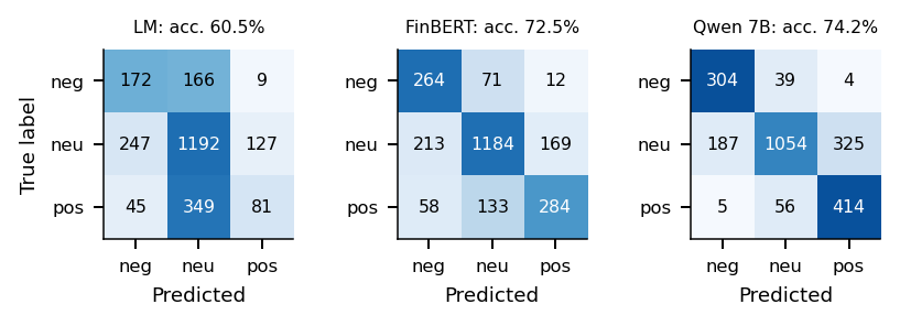
Two of the eleven methods, TF-IDF + LR and MiniLM + LR, are trained on the Twitter training set; all others see no Twitter label. This difference in training data explains most of the ranking on Twitter. On that corpus, all three dictionaries lose to the majority class: GI reaches 43.6%, VADER 49.6% and LM 60.5%, against 66% for "always neutral".
FinBERT reaches 89.0% on PhraseBank and 72.5% on Twitter; zero-shot Qwen2.5-7B reaches 81.4% and 74.2%. The best result on Twitter, 83.2%, comes from the simplest supervised model, TF-IDF + logistic regression. The lesson is that labelled data from the target domain beat model size.
The comparison is one of procedures on two given corpora: it ranks complete pipelines, including their training data, and does not attribute the differences to any single component. Human disagreement and Cohen's \(\kappa\), which corrects agreement for chance, are discussed in Further Topics.
In brief
TF-IDF + LR and MiniLM + LR: the only methods trained on Twitter labels
All three dictionaries lose to the majority class on Twitter
Twitter: GI 43.6%, VADER 49.6%, LM 60.5%; “always neutral”: 66%
FinBERT: 89.0% on PhraseBank, 72.5% on Twitter; Qwen2.5-7B zero-shot: 81.4% and 74.2%
Best on Twitter, 83.2%: the simplest supervised model, TF-IDF + logistic regression
Lesson: labelled data from the target domain beat model size
Type of evidence: comparison of procedures (it shows which method works better on the same data, not why)
Classifiers are compared on two labelled corpora, with accuracy and macro-F1 (15.3), and pairs of classifiers with the McNemar test (15.4), which uses only the texts on which they disagree. On the Twitter headlines, the dictionaries do worse than always answering "neutral", FinBERT and zero-shot Qwen2.5-7B are close (72.5% and 74.2%), and a TF-IDF logistic regression trained on Twitter labels leads with 83.2%.
Language Models: FinBERT and LLMs
Dictionaries give each word a fixed sign. Language models read each word in the context of the sentence. This section describes the fine-tuned model FinBERT, the trap of evaluating it on its own training data, the step from next-word prediction to instruction-following LLMs, and the zero-shot classification of headlines with the Qwen2.5 family.
A dictionary gives "lower" one fixed sign. A language model instead represents each token by a vector that depends on all the other tokens of the sentence, through the attention mechanism of the Transformer (Vaswani et al., 2017), presented in Chapter 14. The representation of "lower" in "lower costs" can then differ from its representation in "lower revenue".
BERT (Bidirectional Encoder Representations from Transformers) (Devlin et al., 2019) is a Transformer encoder pretrained on books and Wikipedia by guessing words hidden at random. It has about 110 million parameters. For classification it uses the final vector \(h_{\text{CLS}} \in \mathbb{R}^{768}\) of a special token, [CLS (classification token of BERT)], placed at the start of every text.
Fine-tuning adds a classification layer on top of \(h_{\text{CLS}}\) and trains the whole network on labelled sentences. The class probabilities and the training loss are
where \(p\) contains the probabilities of the negative, neutral and positive classes, \(y_i\) is the human label of sentence \(i\) and \(\mathcal{L}\) is the cross-entropy. Minimising \(\mathcal{L}\) adjusts both the new layer and the pretrained weights.
BERT (Bidirectional Encoder Representations from Transformers; Devlin et al. (2019))
A Transformer encoder pretrained on books and Wikipedia by guessing words hidden at random
About 110 million parameters
For classification it uses the final vector \(h_{\text{CLS}} \in \mathbb{R}^{768}\) of the special token [CLS (classification token of BERT)] (for classification), placed at the start of every text
Fine-tuning: a classification layer on top of \(h_{\text{CLS}}\)
The whole network is trained on labelled sentences
\(p = \operatorname{softmax}(W h_{\text{CLS}} + c)\), with \(W \in \mathbb{R}^{3 \times 768}\): probabilities of the negative, neutral and positive classes
Training minimises the cross-entropy \(-\frac{1}{n}\sum_i \ln p_{i, y_i}\), with \(y_i\) the human label of sentence \(i\)
FinBERT (Araci, 2019) is BERT further pretrained on financial news and then fine-tuned for sentiment classification. The public model used in this chapter, ProsusAI/finbert, was fine-tuned on Financial PhraseBank. It takes a few milliseconds per sentence on a laptop, which makes it practical for large news archives.
The score used throughout the chapter is the net score (15.1),\(s = p_{\text{pos}} - p_{\text{neg}} \in [-1, 1]\), computed from the probabilities in (15.5), and the predicted label is \(\arg\max_k p_k\). FinBERT is the benchmark because it is public, fast and widely used in the finance literature.
Other versions of the model exist. Huang, Wang & Yang (2023) train a FinBERT on analyst reports, earnings-call transcripts and 10-K filings, and find that it outperforms dictionaries, mainly on sentences that dictionaries misread. The error patterns of FinBERT on the Twitter headlines, compared with those of LM and Qwen2.5-7B, are in Further Topics.
In brief
Araci (2019): FinBERT is BERT further pretrained on financial news, then fine-tuned for sentiment
The public model used here (ProsusAI/finbert) was fine-tuned on Financial PhraseBank
A few milliseconds per sentence on a laptop
The score used in this chapter: \(s = p_{\text{pos}} - p_{\text{neg}} \in [-1, 1]\)
The label is \(\arg\max_k p_k\)
Why FinBERT as the benchmark: public, fast and widely used in the finance literature
Huang, Wang & Yang (2023): a FinBERT trained on analyst reports, earnings-call transcripts and 10-K filings
It outperforms dictionaries, mainly on sentences that dictionaries misread
FinBERT reaches 89.0% accuracy on PhraseBank, but most of PhraseBank was used to train it: Araci (2019) used 3,101 of the 4,845 sentences. On the Twitter headlines its accuracy is 72.5%, a drop of 16.4 points. Part of this drop is genuine difficulty: Qwen2.5-7B, which was not fine-tuned on these labels, also drops, by 7.2 points, because Twitter headlines are harder.
The excess drop of FinBERT is measured by a difference in differences,
which equals 9.2 points, where \(a_{m,D}\) is the accuracy of model \(m\) (F for FinBERT, Q for Qwen) on data \(D\) (P for PhraseBank, T for Twitter). Its bootstrap 95% CI is [6.7; 11.9]. The identifying assumption is that, without training overlap, both models would lose the same amount from PhraseBank to Twitter. The interval measures sampling noise only, not this assumption: the two architectures may react differently to a new domain.
The result supports a descriptive difference between the two accuracy drops. Attributing \(\Delta\) to training overlap would also require an uncontaminated comparator and no other differential change; Qwen was not fine-tuned on PhraseBank, but the texts may be in its pretraining data. The practical rule is the one of the out-of-sample tests of Chapters 8 and 13: a language model is evaluated only on texts it has never seen.
In brief
FinBERT: 89.0% on PhraseBank, most of which it was trained on
Araci (2019): 3,101 of the 4,845 sentences in his version (4 846 here)
72.5% on Twitter: a drop of 16.4 points (from unrounded values)
Qwen2.5-7B, not fine-tuned on these labels, also drops by 7.2 points: Twitter headlines are harder
Shannon (1951) showed that English is highly predictable from its past letters. A large language model (LLM) builds on the same idea: it estimates the conditional distribution \(P(w_{t+1} \mid w_1, \dots, w_t)\) of the next token, where \(w_t\) is the \(t\)-th token, a word or part of a word. Trained on enough text, this single objective produces models that can complete a wide range of tasks.
Brown et al. (2020) showed that, at large scale, such models solve tasks from a few examples placed in the prompt, which is few-shot use. Ouyang et al. (2022) added instruction tuning and RLHF (reinforcement learning from human feedback), which teach the model to follow requests written in plain language. The zero-shot classification used in this chapter relies on this ability.
Domain-specific LLMs also exist. BloombergGPT (Wu et al., 2023) has 50 billion parameters and was trained on financial and general text. Background on next-word prediction and natural language processing is available in the Quantinar courses linked on the slide.
In brief
Shannon (1951): English is highly predictable from its past letters
A large language model (LLM) estimates \(P(w_{t+1} \mid w_1, \dots, w_t)\) over tokens
\(w_t\): the \(t\)-th token, a word or part of a word
Brown et al. (2020): at scale, tasks are solved from a few examples in the prompt (few-shot)
Ouyang et al. (2022): instruction tuning and RLHF (reinforcement learning from human feedback) teach the model to follow requests
BloombergGPT (Wu et al. (2023)): 50 billion parameters, financial and general text
The zero-shot classifier needs no labelled example. The prompt consists of a system instruction, "You classify the sentiment of financial news for investors. Answer with one word: positive, negative or neutral.", followed by the text in the form "Headline: <text> Sentiment:". The model's answer is not generated as free text; instead, the probabilities of the three answer words are read directly.
At the first generated position, let \(z_k\) be the logits of the tokens "positive", "negative" and "neutral". Normalising over these three words gives
\[p_k = \frac{e^{z_k}}{\sum_j e^{z_j}}, \qquad k \in \{\text{pos}, \text{neg}, \text{neu}\}.\]
(15.7)
The label is \(\arg\max_k p_k\), and the score is \(p_{\text{pos}} - p_{\text{neg}}\), as for FinBERT. Reading probabilities rather than parsing generated text makes the classifier deterministic and gives a continuous score that can enter a regression.
In brief
Prompt: a system instruction plus the text to classify
You classify the sentiment of financial news for investors. Answer with one word: positive, negative or neutral.
Headline: <text> Sentiment:
We read the logits \(z_k\) (the model's unnormalised scores) of the tokens “positive”, “negative”, “neutral” at the first generated position
\(p_k = e^{z_k} / \sum_j e^{z_j}\), normalised over the three answer words
Label: \(\arg\max_k p_k\)
Score: \(p_{\text{pos}} - p_{\text{neg}}\), as for FinBERT
When an LLM generates text, it draws the next token from a distribution controlled by the temperature \(T > 0\):
\[p_k(T) = \frac{e^{z_k/T}}{\sum_j e^{z_j/T}}.\]
(15.8)
As \(T \to 0\) the model always chooses the most likely token (greedy decoding) and gives the same answer on every run; Lopez-Lira & Tang (2026) use temperature 0. At \(T = 1\) the model samples from its own distribution, and \(T > 1\) flattens the probabilities, so the answers vary more.
No text is generated in this chapter. The label \(\arg\max_k p_k\) is the answer the model would give as \(T \to 0\), and the score keeps the \(T = 1\) probabilities of (15.7), with nothing to parse. The models are from the Qwen2.5 family (Qwen Team, 2024), open-weight models from 0.5 to 72 billion parameters released on 19 September 2024 under the Apache 2.0 licence, or the Qwen Research License for 3B. The chapter uses 0.5B, 1.5B, 3B, 7B and 14B, where B stands for billion parameters; their processing times are in the Appendix.
Open weights matter for two reasons:
Results can be reproduced with exactly the same model.
The release date of the weights bounds what the model could know, a property used in the section on look-ahead bias.
In brief
When generating, the model draws the next token from \(p_k(T) = e^{z_k/T} / \sum_j e^{z_j/T}\)
With temperature \(T > 0\)
\(T \to 0\): always the most likely token (greedy decoding), so the same answer on every run; Lopez-Lira & Tang (2026) use temperature 0
\(T = 1\): the model's own distribution; \(T > 1\) flattens the probabilities, so answers vary more
No text is generated here: the label \(\arg\max_k p_k\) is the \(T \to 0\) answer
The score keeps the \(T = 1\) probabilities, with nothing to parse
Qwen Team (2024): open-weight models, from 0.5 to 72 billion parameters
Licences: Apache 2.0; Qwen Research License for 3B
Released on 19 September 2024
We use 0.5B, 1.5B, 3B, 7B and 14B (B: billion parameters)
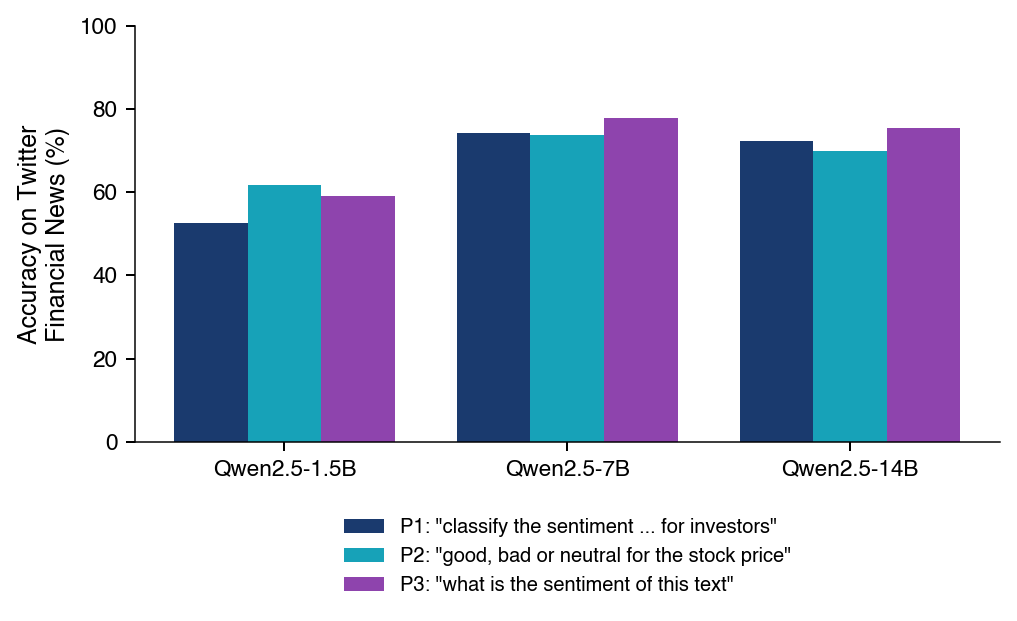
The chart shows the macro-F1 of the five zero-shot Qwen2.5 models, all with the same prompt. The horizontal axis is the number of parameters in billions, on a log scale, and the vertical axis is macro-F1 in percent. The blue line is Financial PhraseBank and the red line Twitter Financial News; the dotted horizontal lines are FinBERT on the two corpora.
In the interactive version, the selector switches between macro-F1 and accuracy, and the slider chooses the prompt used on Twitter, P1, P2 or P3; the three prompts ask the same question in different words. The ▶ button runs through the three prompts. The readout gives the value for 1.5B, 7B, 14B and FinBERT, the share of "neutral" answers of the 1.5B model and the McNemar comparison of 7B with 1.5B.
Question for the room Start at prompt P1 and run ▶ through P3. Among the Qwen2.5 models 1.5B, 7B and 14B, which will have the highest Twitter macro-F1 at P3?
Answer
14B. At P3, macro-F1 is 57.8% for 1.5B, 71.8% for 7B and 73.3% for 14B. At P1, 7B led: 72.6%, against 71.3% for 14B and 55.3% for 1.5B. The ranking also depends on the prompt: the advantage observed at P1 does not automatically carry over to P3.
On PhraseBank, macro-F1 rises with size from 63.3% (0.5B) to 82.1% (14B), still below FinBERT's 88.3%, a lead that is partly training overlap (In-Sample Evaluation Bias). On Twitter the relation is not monotone with prompt P1: 1.5B is the worst model (55.3%) and 7B the best (72.6%), above FinBERT (66.8%) and above 14B (71.3%). In accuracy, 7B beats 1.5B by 21.5 points, with McNemar \(p < 0.001\).
The ranking also depends on the prompt. At P3, macro-F1 is 57.8% for 1.5B, 71.8% for 7B and 73.3% for 14B, so the advantage of 7B at P1 does not carry over. Small models react strongly to wording: with prompt P1 the 1.5B model rarely answers "neutral". The prompt is a parameter of the classifier, discussed in Further Topics.
In brief
Macro-F1 of zero-shot Qwen2.5 with the same prompt; dotted lines: FinBERT
PhraseBank: macro-F1 rises from 63.3% (0.5B) to 82.1% (14B), still below FinBERT (88.3%)
Language models read words in context. FinBERT, a BERT fine-tuned on PhraseBank, looks better on PhraseBank than it is: its excess accuracy drop on Twitter, (15.6), is 9.2 points. Zero-shot LLMs classify from a prompt by reading the probabilities of the answer words, (15.7), without generating text. Their accuracy does not rise monotonically with size and depends on the prompt.
Embeddings as Features
An embedding model maps a text to a generic vector that is not trained for sentiment. A classifier fitted on these vectors with a modest number of labels is a fourth route between dictionaries and fine-tuned models. This section asks whether such vectors contain the sentiment of a headline and how many labels a simple classifier needs.
An embedding is a vector \(e_d \in \mathbb{R}^k\) assigned to text \(d\) such that similar texts have nearby vectors. Word-level embeddings go back to word2vec (Mikolov et al., 2013); Sentence-BERT (Reimers & Gurevych, 2019) produces vectors for whole sentences. The chapter uses MiniLM (Wang et al., 2020), with \(k = 384\) and vectors of unit length, so the similarity of two texts is \(\cos(e_a, e_b) = e_a^\top e_b\). Embeddings enter a classifier or a regression like any other feature.
The chart shows the Twitter validation headlines in the plane of the first two principal components of their MiniLM vectors: the first component on the horizontal axis, the second on the vertical axis, each headline a point coloured by its human label (1,566 neutral, 475 positive and 347 negative). Principal component analysis (PCA), introduced in Chapter 3, keeps the directions of largest variance, not those tied to the label.
In the interactive version, the slider rotates a projection direction within the PC1–PC2 (second Principal Component) plane, from 0° (the first principal component) to 180°, and the second panel shows the positive and negative headlines projected on that direction. The ▶ button rotates the direction step by step; the readout reports the area under the ROC curve (AUC) for positive against negative headlines at the current direction and at the best one.
Question for the room The best direction in the plane of the first two principal components of the MiniLM vectors separates positive from negative headlines with AUC ≈ 0.636. What does this imply about the sentiment information in the embeddings?
Answer
Linear separation in this plane is modest, but the result does not rule out useful information in the other dimensions. PCA maximises explained variance without using the labels. Here the AUC measures only the ranking of positive against negative headlines; it is not three-class accuracy. A logistic regression on all 384 dimensions reaches 78.6% accuracy on Twitter.
The best direction in this plane separates positive from negative headlines with AUC ≈ 0.636, a modest separation. This AUC concerns only the ranking of positive against negative headlines and is not a three-class accuracy. PCA maximises explained variance without using the labels, so the result does not rule out sentiment information in the other dimensions. A logistic regression on all 384 dimensions finds the sentiment direction and reaches 78.6% accuracy on Twitter.
In brief
Embedding: a vector \(e_d \in \mathbb{R}^k\), close for similar texts
Here MiniLM (Wang et al. (2020)), \(k = 384\), unit length: similarity \(\cos(e_a, e_b) = e_a^\top e_b\); embeddings enter a classifier or regression like any feature
Chart: Twitter validation headlines, first two principal components of the MiniLM vectors
Coloured by label
The first two components do not separate sentiment
PCA (principal component analysis, Chapter 3) keeps the directions of largest variance
Not those tied to the label
A logistic regression on all 384 dimensions finds the sentiment direction: 78.6% accuracy on Twitter
A classifier on embeddings or on TF-IDF features needs labels from the target domain, and the learning curve shows how its accuracy grows with their number. The horizontal axis is the number of labelled training headlines, on a log scale from 100 to the full Twitter training set; the vertical axis is the accuracy on the validation set in percent. The two coloured lines are MiniLM embeddings + logistic regression and TF-IDF + logistic regression, each with a band of \(\pm 2\) standard deviations across training resamples. The horizontal lines are FinBERT and Qwen2.5-7B, which use no Twitter labels.
In the interactive version, the slider steps through the tested numbers of training labels, and the ▶ button moves along the curve. The readout reports the mean accuracy of both classifiers at the chosen size and compares them with FinBERT.
Question for the room What is the first tested number of Twitter labels at which MiniLM + LR's mean accuracy across training resamples exceeds FinBERT?
Answer
400. The mean is 71.9% at 200 labels and 73.3% at 400; FinBERT has 72.5%. Some training runs already beat the benchmark at 200, and at 800 all ten do. The threshold of 400 concerns the mean, not every sample. TF-IDF starts lower (66.9% at 100 labels) but reaches about 83% with all 9,543 labels, against 78.6% for embeddings.
The mean accuracy of MiniLM + LR is 71.9% at 200 labels and 73.3% at 400, against 72.5% for FinBERT: 400 is the first tested size at which the mean exceeds the benchmark. Some training runs already beat FinBERT at 200 labels, and at 800 all ten do. The threshold of 400 concerns the mean, not every sample.
Each point of the curve comes from a logistic regression trained on a random subset of the Twitter training set of the given size, with 10 repetitions per size; the band covers \(\pm 2\) standard deviations across the repetitions. The design measures how much the result depends on which headlines happen to be labelled, as well as on how many.
Embeddings + logistic regression start high: 69.0% with 100 labels, and above FinBERT from 400 labels. The pretrained vectors already contain most of what the classifier needs, and a few hundred labels suffice to find the sentiment direction. TF-IDF starts lower, at 66.9%, but keeps improving and reaches about 83% with all labels, against 78.6% for embeddings. With many labels, exact words such as "upgrade", "cuts" or "misses" carry the signal in headlines, and a sparse word representation can use them directly.
The practical rule is to label a few hundred documents from one's own domain before trusting any off-the-shelf model. The same labelled sample serves later as the validation sample of the section on scores as estimates.
In brief
Logistic regression trained on random subsets of the Twitter training set
10 repetitions per size; band: \(\pm 2\) standard deviations
Embeddings + logistic regression: 69.0% with 100 labels, above FinBERT from 400 labels
The pretrained vectors already contain most of what is needed
TF-IDF starts lower (66.9%) but keeps improving
About 83% with all labels, against 78.6% for embeddings
With many labels, exact words (“upgrade”, “cuts”, “misses”) carry the signal in headlines
Practical rule: label a few hundred documents from your own domain
Generic MiniLM vectors do not separate sentiment in their first two principal components, but a logistic regression on all 384 dimensions reaches 78.6% on Twitter and exceeds FinBERT in mean accuracy from 400 labels. With the full training set, TF-IDF does better still, at about 83%. A few hundred labels from the domain are worth more than a larger general model.
Look-Ahead Bias and Memorisation
An LLM is trained on text that may describe the events a backtest tries to forecast. This section states the problem, presents a direct test of what Qwen2.5 remembers about past market moves, and lists the remedies.
An LLM trained on text up to 2024 may have read what happened after a headline published in 2015. A backtest on 2015 news then mixes forecasting with remembering: a high score may reflect knowledge of the subsequent price path rather than a reading of the headline.
Glasserman & Lin (2023) identify two biases in sentiment backtests with LLMs. Look-ahead bias arises when the model knows the returns that followed the news. Distraction arises when general knowledge about the named company interferes with reading the text; in their tests, distraction mattered more than look-ahead. Sarkar & Vafa (2024) show, with direct tests, that look-ahead is present in LLM applications to earnings calls and elections.
Every backtest of LLM scores on headlines that predate the model's release therefore needs a statement of what the model could have known, and preferably a test of it.
In brief
An LLM trained on text up to 2024 may have read what happened after a 2015 headline
A backtest on 2015 news then mixes forecasting with remembering
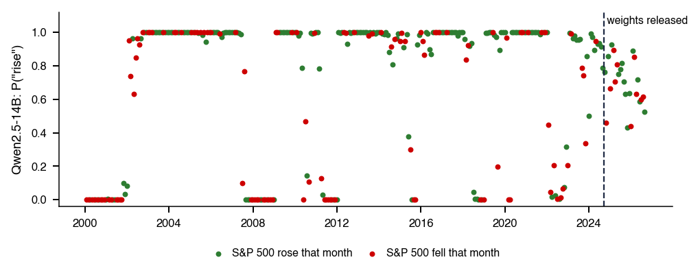
The test asks the model about past market moves without giving it any text to read. In the monthly version the question is "Did the S&P 500 index rise or fall during <month year>?", asked for every month in 296 months before the release of the weights and 23 months after it. In the daily version the question is "Did Apple stock close higher or lower on <date> than on the previous trading day?", asked for 500 random days from 2010–2023 and 493 days after October 2024.
The score is \(P(\text{rise})\), computed from the probabilities of the answer words as in (15.7). The true direction comes from the monthly closes of the S&P 500 and the daily closes of Apple. Discrimination is measured by the AUC, the area under the ROC (receiver operating characteristic) curve: the probability that a randomly chosen up period receives a higher score than a randomly chosen down period. An AUC of 0.5 means no discrimination; the metric is presented in Chapter 13.
After the release there is nothing to remember. If the date carries no predictive information, for example through seasonality, the population AUC after the release is 0.5 and the sample AUC varies around it. The months after the release thus act as a control for the months before.
In brief
Monthly: “Did the S&P 500 index rise or fall during <month year>?”
Every month from 296 pre-release months plus 23 after
Daily: “Did Apple stock close higher or lower on <date> than on the previous trading day?”, 500 random days 2010–2023 and 493 days after October 2024
Score: \(P(\text{rise})\) from the answer-word probabilities
True direction from the S&P 500 monthly closes and the Apple daily closes
AUC (area under the ROC curve; ROC: receiver operating characteristic): probability that a random up period gets a higher score than a random down period; 0.5 = no discrimination (Chapter 13)
After the release there is nothing to remember
If the date carries no predictive information (e.g. seasonality), the population AUC is 0.5
The chart reports the AUC of three Qwen2.5 models, 1.5B, 7B and 14B, with 95% intervals. The left panel concerns the direction of S&P 500 months and the right panel the direction of single Apple days; the horizontal axis is the model size and the vertical axis the AUC. Blue points are periods before the weights were released, orange points periods after the release, when the model cannot know the answer. The dashed line marks 0.5.
In the interactive version, the first selector chooses the series (S&P 500 months or Apple days) and the second the model. The slider sets the threshold above which an answer counts as "rise", and the second panel shows the corresponding point on the ROC curve; the ▶ button moves the threshold from 0 to 1 and traces the curve.
Question for the room For Qwen2.5-14B, the AUC on the S&P 500 months before the weights were released is 0.69, with a 95% CI of [0.62; 0.75]. What conclusion does this result support?
Answer
Discrimination above 0.5, consistent with memorisation, without identifying the mechanism on its own. The result measures how well past months are discriminated: it does not separate memorisation from calendar or regime regularities, nor does it establish future performance. For single days of Apple, the AUC stays between 0.48 and 0.52. On the 23 months after the release, the AUC is 0.59, with a wide interval, approximately [0.35; 0.84]: about 101 months would be needed.
For Qwen2.5-14B, the AUC on the S&P 500 months before the release is 0.69, with 95% CI [0.62; 0.75]. This is discrimination above 0.5, consistent with memorisation, but it does not identify the mechanism on its own: it does not separate memorisation from calendar or regime regularities, and it says nothing about future months. For single Apple days the AUC stays between 0.48 and 0.52. On the 23 months after the release, the AUC of 14B is 0.59, with a wide interval of about [0.35; 0.84].
The intervals are bootstrap 95% intervals, with months resampled independently. Before the release, the AUC is 0.67 for 7B (CI [0.61; 0.73]) and 0.69 for 14B (CI [0.62; 0.75]), and the permutation p-value for 14B is below 0.001. The 1.5B model knows much less, with an AUC of 0.57.
After the release, on 23 months, the intervals include 0.5, but they are too wide to prove anything. About 101 post-release months would be needed to detect a fall from 0.69 to 0.5; the formal test and its power are in the Appendix. For single Apple days, the AUC lies between 0.48 and 0.52 before the release: no discrimination above chance is detected.
Look-ahead is thus a danger at the horizon of well-known events, such as the direction of a month remembered for a crash, and less so for daily noise. The result is descriptive: the discrimination of months is compatible with memorisation but does not separate it from calendar or regime regularities. The month-by-month answers of 14B are shown in Further Topics.
In brief
AUC with bootstrap 95% intervals, months resampled independently
Months before release: AUC 0.67 (7B, CI [0.61; 0.73]) and 0.69 (14B, CI [0.62; 0.75])
Permutation \(p\) for 14B \(<\)0.001
The 1.5B model knows much less (0.57)
After release (23 months) the intervals include 0.5 but are too wide to prove anything
About 101 post-release months would be needed to detect a fall to 0.5 (formal test: Appendix)
Single days of Apple: AUC between 0.48 and 0.52 before release, no discrimination above chance detected
Look-ahead is a danger at the horizon of well-known events, less for daily noise
Type of evidence: description; the discrimination of months is compatible with memorisation but does not separate it from calendar or regime regularities
Testing only on news published after the model's training cutoff, the cleanest remedy. Lopez-Lira & Tang (2026) evaluate GPT-4 on headlines published after its cutoff; the design is clean, but the evaluation window starts late.
Masking company names and dates before scoring and comparing slopes with and without masking (Glasserman & Lin, 2023). This is a diagnostic rather than a cure, since products, events or quotes can still identify the episode.
A point-in-time model, trained only on text available up to the date \(t\) of the analysis (Sarkar & Vafa, 2024).Drinkall et al. (2024) release a series of point-in-time LLMs, each uninformed about facts after its date, with public models and training data. He et al. (2025) build ChronoBERT and ChronoGPT, which use only text available at each date; on next-day returns from news, their Sharpe ratios are close to those of a much larger model, so look-ahead is modest in that application.
Whatever remedy is chosen, every result should state the model version and the release date of its weights, so that the reader can judge what the model could have known.
A diagnostic, since products, events or quotes can still identify the episode
Point-in-time models, trained only on text available up to date \(t\) (Sarkar & Vafa (2024))
Drinkall et al. (2024): a series of point-in-time LLMs, each uninformed about facts after its date; models and training data are public
He et al. (2025): ChronoBERT and ChronoGPT use only text available at each date; on next-day returns from news their Sharpe ratios are close to a much larger model: look-ahead there is modest
Report the model version and the release date of its weights with every result
Section summary
Asked only for the month, Qwen2.5-14B separates up from down months of the S&P 500 before its release with an AUC of 0.69, while single Apple days are not discriminated. The 23 post-release months are too few to show whether the discrimination vanishes. Backtests of LLM scores therefore need post-release data, masking diagnostics or point-in-time models, and a statement of the model's release date.
From Sentiment to a Trading Signal
The previous sections measured how well scores agree with human labels. This section asks whether the tone of dated headlines predicts returns that can still be traded. It describes the FNSPID headlines and their timestamps, the pooled regression and its inference with 16 stocks, and a daily long-short strategy after costs.
The data come from FNSPID, the Financial News and Stock Price Integration Dataset (Dong, Fan & Peng, 2024): 15.7 million news records about S&P 500 firms from four news websites, covering 1999–2023, under the Creative Commons licence CC BY-NC 4.0 (attribution, non-commercial use).
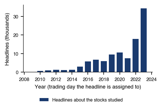
The chapter uses 16 large US stocks for which daily prices are available in the course data: technology firms, banks, GameStop and Strategy. After repeated headlines are removed, there are 106,820 distinct headlines and 18,282 stock-days with news, from 27 October 2009 to 18 December 2023. Coverage is uneven over time, as Further Topics shows.
The sample is small in the cross-section and selected: 16 heavily followed large firms, chosen among today's survivors. Both features matter for the interpretation of the results that follow.
In brief
The question of this section: does headline tone predict returns that we can still trade?
The timing of a headline relative to the trading session decides which return it can predict. The chart shows the distribution of the FNSPID timestamps by hour. The horizontal axis is the hour of the timestamp in Coordinated Universal Time (UTC), the vertical axis the number of headlines on a log scale; the red bar is midnight, 00:00 UTC.
In the interactive version, the slider moves the clock from UTC to another time zone, with offsets from −12 to +12 hours, and the ▶ button steps through the offsets.
Question for the room If we move the clock from UTC to UTC−5, do we learn whether the FNSPID headlines appeared before or after the close?
Answer
No. 99.8% of the headlines are stamped exactly 00:00 UTC, so the source gives only the date. At UTC−5, 00:00 UTC becomes 19:00 on the previous day, but the conversion only changes how the stamp is displayed, without adding the publication time. The returns of days d and d+1 may therefore still contain the reaction, and the first return used as a tradable forecast is that of day d+2.
Moving the clock does not reveal whether a headline appeared before or after the close. 99.8% of the headlines are stamped exactly 00:00 UTC, so the source gives only the date. At UTC−5, 00:00 UTC becomes 19:00 on the previous day, but the conversion only changes how the stamp is displayed; it adds no publication time.
Because 99.8% of headlines carry the stamp 00:00 UTC, the source records the date of publication, not its time. A headline dated \(d\) may have appeared before the open, during the session or after the close of day \(d\). Any alignment of headlines with returns has to be valid in all three cases.
The alignment used in the chapter assigns each headline to day \(d\), the first trading day on or after its date. Returns on \(d\) and on \(d+1\) may still contain the reaction to the news: on \(d\) if the headline appeared before or during the session, on \(d+1\) if it appeared after the close. The first safe forecast is the return on \(d+2\), from the close of \(d+1\) to the close of \(d+2\). This alignment has no look-ahead, at the price of discarding the first day after the news.
In brief
Hour of the FNSPID timestamp in Coordinated Universal Time (UTC), log scale
99.8% of headlines are stamped exactly 00:00 UTC
The source gives the date, not the time of publication
A headline dated \(d\) may have appeared before the open, during the session or after the close of day \(d\)
Alignment used here, with no look-ahead
Day \(d\): the first trading day on or after the date of the headline
Returns on \(d\) and \(d+1\) may still contain the reaction
First safe forecast: the return on \(d+2\), close of \(d+1\) to close of \(d+2\)
Three scores are computed for every headline: the LM tone (15.2), the FinBERT net score \(P(\text{pos}) - P(\text{neg})\), and the Qwen2.5-7B net score with prompt P1. The LM dictionary finds a listed word in only 27% of the headlines; all the others receive tone 0. The FinBERT labels are 19% negative, 62% neutral and 18% positive.
The scores agree only partly. Across headlines, the correlation is 0.62 between FinBERT and Qwen, 0.41 between FinBERT and LM and 0.36 between Qwen and LM. The two language models are closer to each other than either is to the dictionary.
The outcome is the excess return of stock \(i\) on day \(t\) over SPY, an exchange-traded fund that tracks the S&P 500 index:
\[r^{e}_{i,t} = r_{i,t} - r_{\text{SPY},t}.\]
(15.9)
This market-adjusted return sets \(\beta = 1\) for every stock. The usual alternative is \(r_{i,t} - \hat\alpha_i - \hat\beta_i r_{\text{SPY},t}\), with \(\hat\beta_i\) estimated before the event.
In brief
The three scores: LM tone, FinBERT net score and Qwen2.5-7B net score with prompt P1 (the one on the zero-shot classification slide)
FinBERT net score: \(P(\text{pos}) - P(\text{neg})\)
LM finds a listed word in only 27% of headlines: the rest get tone 0
SPY: an exchange-traded fund tracking the S&P 500 index
Market-adjusted: \(\beta = 1\) for every stock; the usual alternative is \(r_{i,t} - \hat\alpha_i - \hat\beta_i r_{\text{SPY},t}\), with \(\hat\beta_i\) estimated before the event
The Regression and Standard Errors Clustered by Day
The relation between scores and returns is estimated by a pooled regression over the stock-days with news:
\[r^{e}_{i,d+h} = a + b\,z_{i,d} + \varepsilon_{i,d+h}, \qquad h = 0, 1, 2,\]
(15.10)
where \(z_{i,d}\) is the daily score of stock \(i\) on day \(d\), standardised over the panel to mean 0 and standard deviation 1. The slope \(b\) is then the excess return, in percent, per one standard deviation of the score. The horizon \(h = 0\) measures the reaction on the news day, and \(h = 2\) measures predictability, since \(d+2\) is the first safe return.
The errors of different stocks on the same day are correlated through common market shocks. Ordinary least squares (OLS) standard errors ignore this correlation and are too small. Following Petersen (2009), the variance is clustered by day:
where \(g\) indexes trading days, \(X\) contains the regressors (a constant and \(z\)), and \(X_g\) and \(\hat\varepsilon_g\) are the rows and OLS residuals of day \(g\). The middle term allows any correlation among the residuals of one day and none across days.
In brief
Pooled regression over stock-days with news: \(r^{e}_{i,d+h} = a + b\,z_{i,d} + \varepsilon_{i,d+h}\), \(h = 0, 1, 2\)
\(z\): daily score standardised over the panel (mean 0, standard deviation 1), so \(b\) is the excess return (%) per one standard deviation of score
The chart reports the slope \(b\) of (15.10) for each of the three scores and three horizons. The horizontal axis lists the scores (Loughran–McDonald tone, FinBERT, Qwen2.5-7B); the vertical axis is the excess return in basis points (bp, 1 bp = 0.01%) per one standard deviation of the score, with 95% intervals clustered by day. Blue is the news day \(d\), ochre the day \(d+1\), when news may still be arriving, and red the day \(d+2\), the tradable forecast.
In the interactive version, the slider sets the minimum number of headlines per stock-day that enters the regression, from 1 to 20, and the selector chooses the horizons, \(d\) to \(d+2\) or \(d\) to \(d+5\). The ▶ button raises the minimum number of headlines step by step.
Question for the room With the initial filter of at least one headline per stock-day, what conclusion do the slope estimates for the excess return of day d+2 support?
Answer
We do not detect slopes different from zero at the two-sided 5% level, with standard errors clustered by day. The t-statistics are −0.25 for FinBERT, +1.19 for Qwen and −0.01 for LM; none exceeds the asymptotic reference value 1.96 in absolute value. This is a lack of evidence in this specification, not proof of exactly zero effects. On day d the slopes are large: FinBERT +39.2 bp (t = 17.27) and Qwen +41.4 bp (t = 19.07); many headlines report the price move itself.
On day \(d\) the slopes are large: FinBERT +39.2 bp (\(t\) = +17.27), Qwen +41.4 bp (\(t\) = +19.07) and LM +15.5 bp (\(t\) = +8.53). Many headlines report the price move itself ("shares jump", "stock falls"), so causality runs both ways. On day \(d+1\) the slopes are +3.2 bp for FinBERT (\(t\) = +1.60) and +3.7 bp for Qwen (\(t\) = +1.86); part of this is news published after the close of \(d\), not a forecast.
On day \(d+2\) the slopes are −0.5 bp for FinBERT (\(t\) = −0.25), +2.3 bp for Qwen (\(t\) = +1.19) and −0.0 bp for LM (\(t\) = −0.01). None exceeds 1.96 in absolute value: we do not detect slopes different from zero at the two-sided 5% level, with standard errors clustered by day. This is a lack of evidence in this specification, not proof of exactly zero effects.
In brief
Slope \(b\) in basis points (bp, 1 bp = 0.01%) per one standard deviation of score (s.d. in the chart)
95% CI clustered by day
Day \(d\): FinBERT +39.2 bp (\(t\) = +17.27), Qwen +41.4 bp (\(t\) = +19.07), LM +15.5 bp (\(t\) = +8.53)
Many headlines report the price move itself (“shares jump”, “stock falls”): causality runs both ways
Day \(d+1\): FinBERT +3.2 bp (\(t\) = +1.60), Qwen +3.7 bp (\(t\) = +1.86)
Part of this is news published after the close of \(d\), not a forecast
Day \(d+2\): FinBERT \(-\)0.5 bp (\(t\) = \(-\)0.25), Qwen +2.3 bp (\(t\) = +1.19), LM \(-\)0.0 bp (\(t\) = \(-\)0.01)
Clustering by day handles common shocks, but the errors of one stock may also be correlated across days, because firm effects persist. The slopes therefore have to survive clustering by stock as well. Two-way clustering (Cameron, Gelbach & Miller, 2011) combines the two:
where each term is the sandwich (15.11) with clusters given by day, by stock and by the stock–day pair respectively.
A stock–day pair contains a single observation here, so the last term is the White estimator, robust only to heteroskedasticity. Subtracting it avoids counting the variance of each observation twice, since both the day and the stock clusters include it. Driscoll & Kraay (1998) also allow for correlation across different days.
In brief
The question: do the slopes survive if errors are also correlated over time within a stock?
Firm effects persist, so the errors of one stock are correlated across days: cluster by stock as well
Clustering by stock leaves only \(G = 16\) clusters. With so few clusters, the stock-clustered standard error is too small and the \(t\) test rejects too often (Cameron, Gelbach & Miller, 2008). The wild cluster bootstrap with the null imposed corrects this.
The procedure first fits the restricted model with \(b = 0\), which gives a constant \(\tilde a\) and residuals \(\tilde\varepsilon_{i,t}\). For \(j = 1, \dots, B\), with \(B = 9{,}999\), it draws Rademacher weights \(w_g = \pm 1\) with probability \(\tfrac12\) each, one draw per stock \(g\), builds the bootstrap returns \(r^{e*}_{i,t} = \tilde a + w_{g(i)}\,\tilde\varepsilon_{i,t}\), re-fits the regression and computes the stock-clustered statistic \(t^*_j\). The p-value is
Giving all residuals of a stock the same sign keeps the correlation within the cluster. The bootstrap assumes that stocks are independent, so it is read next to the two-way statistic, which allows correlation across stocks on the same day.
In brief
With only \(G = 16\) stocks, the stock-clustered SE (Standard Error) is too small and the \(t\) test rejects too often (Cameron, Gelbach & Miller (2008))
Wild cluster bootstrap (resampling with random signs per cluster) with the null imposed: fit the restricted model (\(b = 0\))
Constant \(\tilde a\) and residuals \(\tilde\varepsilon_{i,t}\)
For \(j = 1, \dots, B\), \(B = 9{,}999\): Rademacher weights \(w_g = \pm 1\) with probability \(\frac12\), one draw per stock \(g\)
\(r^{e*}_{i,t} = \tilde a + w_{g(i)}\,\tilde\varepsilon_{i,t}\); re-fit the regression and compute the stock-clustered \(t^*_j\)
The analysis runs nine regressions: three scores times three horizons, \(h = 0, 1, 2\). If no score had any effect, nine tests at 5% would still give \(9 \times 0.05 = 0.45\) false rejections on average. The family of tests needs a correction for multiple testing.
The Holm correction, presented in Chapter 2, keeps the family-wise error rate (FWER), the probability of any false rejection, at or below 5%. With the p-values sorted, \(p_{(1)} \le \dots \le p_{(m)}\) and \(m = 9\), the adjusted p-values are
and \(H_{(k)}\) is rejected when \(\tilde p_{(k)} \le 0.05\). Holm is more powerful than Bonferroni, which multiplies every p-value by \(m\), and remains valid under any dependence between the tests.
The table reports, for the main combinations of score and horizon, the slope in basis points, the \(t\) statistic clustered by stock, the two-way statistic (15.12), the wild-bootstrap p-value (15.13) and the Holm-adjusted p-value (15.14). The same-day slopes survive every correction: FinBERT +39.2 bp, with \(t\) = +5.71 by stock and +5.67 two-way, and Qwen +41.4 bp, with +5.10 and +5.07; their bootstrap and Holm p-values are below 0.001.
The tradable horizon is different. Qwen at \(d+2\) has \(t\) = +2.41 by stock, which looks significant: \(p\) = 0.029 under a \(t\) distribution with 15 degrees of freedom. The wild bootstrap gives \(p\) = 0.061, and Holm then gives 0.37. Among the nine sorted bootstrap p-values, Qwen at \(d+2\) comes fourth, after the three same-day values, all below 0.001, so its Holm p-value is \((9 - 4 + 1) \times 0.061 \approx 0.37\). FinBERT and LM at \(d+2\) have Holm p-values of 1.00. The rows not shown are LM at \(d\), with \(p < 0.001\), and the three slopes at \(d+1\), with \(p\) = 0.272 (FinBERT), 0.317 (Qwen) and 0.802 (LM).
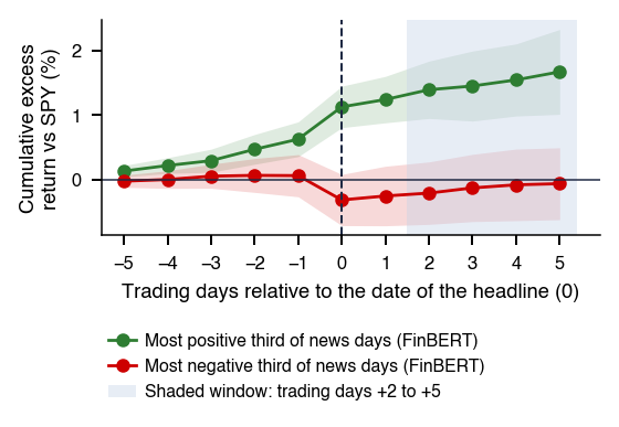
The result supports association: scores and same-day returns move together, but the direction of causality is open. The event study in Further Topics shows that the stock-days with the most positive scores already gain +0.63% in the 5 days before the news.
In brief
Score, horizon
\(b\) (bp)
\(t\) by stock
\(t\) two-way
\(p\) wild bootstrap
\(p\) Holm
FinBERT, \(d\)
+39.2
+5.71
+5.67
\(<\)0.001
\(<\)0.001
Qwen, \(d\)
+41.4
+5.10
+5.07
\(<\)0.001
\(<\)0.001
FinBERT, \(d+2\)
\(-\)0.5
\(-\)0.35
\(-\)0.30
0.739
1.00
Qwen, \(d+2\)
+2.3
+2.41
+2.01
0.061
0.37
LM, \(d+2\)
\(-\)0.0
\(-\)0.03
\(-\)0.02
0.979
1.00
Qwen at \(d+2\): \(t\) = +2.41 by stock looks significant
\(p\) = 0.029 under a \(t\) distribution with 15 degrees of freedom
But not after the wild bootstrap and Holm
Holm step by step: sort the 9 bootstrap \(p\)-values; Qwen at \(d+2\) comes 4th, after the three same-day values (all below 0.001), so its Holm \(p\) = (9 \(-\) 4 + 1) \(\times\) 0.061 \(\approx\) 0.37
Rows not shown: LM at \(d\), \(p\)\(<\)0.001; at \(d+1\), \(p\) = 0.272 (FinBERT), 0.317 (Qwen), 0.802 (LM)
Type of evidence: association (the variables move together; this does not prove causation)
The most positive third of scores already has a cumulative excess return of +0.63% in the 5 days before the news (Further Topics)
The regression measures association; a strategy asks whether the sign of the score earns a profit that can actually be collected. At the close of \(d+1\), for every stock with news and a non-zero score on day \(d\), the strategy goes long if the score is positive and short if it is negative. Each position is hedged with SPY; a one-for-one hedge removes the market move only when \(\beta = 1\). Positions have equal weights and are closed after one day, at the close of \(d+2\). The LM score is zero on 48% of stock-days, and these stock-days do not enter the portfolio.
The gross return of the strategy on day \(d+2\) is
where \(A_d = \{i : |s_{i,d}| > b\}\) is the set of stocks with news and a score above the threshold \(b\) in absolute value, here \(b = 0\), and \(N_d = |A_d|\) is the number of positions opened at the close of \(d+1\). If \(A_d\) is empty, \(G_{d+2} = 0\) and no costs are paid.
In brief
The question: does the sign of the score earn a profit we can actually collect?
At the close of \(d+1\): for every stock with news and a non-zero score on \(d\), go long or short
Long if its score is positive and short if negative
Each position hedged with SPY; a one-for-one hedge removes the market move only when \(\beta = 1\)
Equal weights; positions are closed after one day, at the close of \(d+2\)
The LM score is zero on 48% of stock-days: these do not enter the portfolio
The cost of trading is set at \(c\) = 5 bp per one-way trade, per unit of traded notional. The value is assumed, not estimated; it is plausible for large, liquid US stocks. A round trip, entering and leaving a position, costs \(2c\). On a day with positions the strategy makes one round trip for the stock book and one for the SPY hedge, each of notional 1, so it pays \(4c\) = 20 bp.
The break-even cost \(c^*\) is the value of \(c\) at which the mean net return is zero, \(c^* = \bar G_{\text{active}}/4\), where \(\bar G_{\text{active}}\) is the mean gross return on the days with positions. A strategy is worth trading only if its break-even cost exceeds the cost the trader actually pays.
In brief
\(c\) = 5 bp per one-way trade, per unit of traded notional
Assumed, not estimated; plausible for large, liquid US stocks
A round trip (in and out) costs \(2c\)
On a day with positions: one round trip for the stock book and one for the SPY hedge
Each of notional 1, so \(4c\) = 20 bp
Net return: \(G^{\text{net}}_{d+2} = G_{d+2} - 4c\,\mathbf{1}\{N_d > 0\}\)
Break-even cost \(c^*\): the value of \(c\) at which the mean net return is 0
I.e. \(c^* = \bar G_{\text{active}}/4\)
\(\bar G_{\text{active}}\): the mean gross return on days with positions
Reading the Strategy Numbers: Sharpe Ratio and Summed Returns
Inference on the mean daily return uses the Newey–West \(t\) statistic, presented in Chapter 2, and a block-bootstrap confidence interval. Both allow for serial correlation of the daily returns.
The annualised Sharpe ratio is
\[SR = \sqrt{252}\,\frac{\bar G}{\hat\sigma},\]
(15.17)
where \(\bar G\) and \(\hat\sigma\) are the mean and standard deviation of the daily return \(G_t\) over all 3,568 trading days; days without positions enter as 0, and after costs \(G_t\) is replaced by the net return (15.16). For Qwen2.5-7B, a mean of +5.64 bp and \(SR\) = +0.63 imply \(\hat\sigma = \sqrt{252} \times \text{mean}/SR \approx 143\) bp per day.
The effect of costs follows from (15.16): with positions on 95% of days, the mean falls by \(20 \times 0.95\) bp. The next chart sums the daily simple excess returns; the sum is an additive measure of profit, not compounded wealth.
In brief
Inference: Newey–West \(t\) (Chapter 2) and block-bootstrap CI for the mean daily return
Sharpe ratio \(SR = \sqrt{252}\,\bar G / \hat\sigma\) (annualised)
\(\bar G\), \(\hat\sigma\) are the mean and standard deviation of the daily return \(G_t\) over all 3 568 trading days
Days without positions enter as 0
After costs, \(G_t\) is replaced by the net return
Example (Qwen2.5-7B): mean +5.64 bp and \(SR\) = +0.63 imply \(\hat\sigma = \sqrt{252} \times\) mean\(/SR \approx\) 143 bp per day
After costs: positions on 95% of days, so the mean falls by \(20 \times\) 0.95 bp, to \(-\)13.36 bp per day
The chart shows the cumulative sum of the daily excess returns of the strategy (15.15), in percent, from 2010 to 2024. Solid lines are gross returns and dashed lines net returns with 5 bp per one-way trade; orange is the LM score, blue FinBERT and red Qwen2.5-7B.
In the interactive version, the first slider chooses the return day, from \(d+1\) to \(d+5\), the second the cost per one-way trade, from 0 to 10 bp, and the third the last day included in the sum. The ▶ button extends the sum through time.
Question for the room For the Qwen2.5-7B strategy on d+2, the gross mean is 5.64 bp a day and about 95% of the days are active. With a one-way cost c = 5 bp per trade, what is the net mean?
Answer
About −13.36 bp a day. An active day pays 4c: entry and exit for the stock position and for the SPY hedge. The net mean is 5.64 − 0.95 × 4 × 5 ≈ −13.36 bp. +0.89 bp counts a single direction; −3.86 bp counts a single round trip. The Sharpe ratio falls from +0.63 to −1.48, and the break-even cost is 1.5 bp per trade.
Before costs, FinBERT earns +3.27 bp per day (\(t\) = +1.27), with 95% CI [−1.51; +8.93], not different from zero; LM earns −0.21 bp (\(t\) = −0.07). Qwen2.5-7B earns +5.64 bp per day (\(t\) = +2.26, \(p\) = 0.024), with CI [+0.95; +10.61]. As the best of three scores, its Holm p-value is 0.071, not significant.
Costs remove the gain. An active day pays \(4c\), and with active days on about 95% of days the net mean is \(5.64 - 0.95 \times 4 \times 5 \approx -13.36\) bp a day. The break-even cost of Qwen2.5-7B is 1.5 bp per trade, well below 5 bp, and its Sharpe ratio falls from +0.63 before costs to −1.48 after costs. The result supports association only: the large gains are concentrated in 2020–2021 and are not significant at 5% (Further Topics).
In brief
Sum of daily excess returns (%), before costs and with 5 bp per trade
FinBERT: +3.27 bp per day (\(t\) = +1.27), not different from zero
CI 95% [\(-\)1.51; +8.93]; LM: \(-\)0.21 bp (\(t\) = \(-\)0.07)
Qwen2.5-7B: +5.64 bp (\(t\) = +2.26, \(p\) = 0.024)
CI 95% [+0.95; +10.61]; but it is the best of the three scores tested: Holm \(p\) across the three = 0.071, not significant
Break-even cost +1.5 bp per trade, well below 5 bp: Sharpe +0.63 before, \(-\)1.48 after costs
Type of evidence: association
Only 2020–2021 has large gains, not significant at 5% (Further Topics)
The strategy on the non-tradable day \(d+1\) checks the timing. FinBERT earns −0.22 bp (\(t\) = −0.10) and Qwen +4.06 bp (\(t\) = +1.36). There is no significant gain even on that day: almost all of the reaction happens on day \(d\), which the date-only timestamps make impossible to trade.
Part of the Qwen edge may be memorised. The Qwen2.5 weights were released on 19 September 2024, and every headline in the sample, from 2010 to 2023, predates them. A headline that names an episode can trigger recall of what followed, unlike the Apple test of the previous section, which gave only the date. The memory test bounds what the model knows about dates; it does not bound what it knows about named events.
In brief
Non-tradable day \(d+1\): FinBERT \(-\)0.22 bp (\(t\) = \(-\)0.10), Qwen +4.06 bp (\(t\) = +1.36)
No significant gain even there: almost all of the reaction happens on day \(d\)
Part of the Qwen edge may be memorised: the Qwen2.5 weights were released on 19 September 2024, after the 2010–2023 headlines
A headline that names the episode can trigger recall, unlike the Apple test, which gave only the date
Headline scores explain the same-day move: +39.2 bp per standard deviation for FinBERT and +41.4 bp for Qwen, robust to two-way clustering, the wild bootstrap and Holm. The relation reflects in large part headlines that describe price moves. At the first safe horizon, \(d+2\), no slope survives the corrections, and the daily long-short strategy brings no net profit: the best score, Qwen2.5-7B, breaks even at 1.5 bp per trade, below the assumed cost of 5 bp.
Measurement Error in Sentiment Scores
A sentiment score is the output of a model, not the true tone of the text. When it enters a regression as a regressor, or when its mean is reported as a population quantity, the measurement error of the score passes into the estimates. This section derives the attenuation of a slope on a generated regressor, measures it for the chapter's three scores, and presents prediction-powered inference, which builds valid intervals from model scores and a small human-labelled sample.
Sentiment as a Generated Regressor: Classical Error
The question of the section is what happens to the slope and its interval when the regressor is a model output rather than the true tone. Let the true model be \(r = a + \beta s^* + \varepsilon\), where \(s^*\) is the true tone of the text. We observe only a model output \(\hat s = s^* + u\), where \(u\) is the measurement error.
Under classical error, \(u\) is independent of \(s^*\) and of \(\varepsilon\). The OLS slope of \(r\) on \(\hat s\) then converges to
where \(\lambda\) is the reliability of the score, the share of its variance that is signal. The slope is attenuated towards zero by the factor \(\lambda\).
Two consequences follow. The test of \(\beta = 0\) remains valid, because \(\beta\lambda = 0\) exactly when \(\beta = 0\). The magnitude, however, is understated: a slope estimated on a noisy score underestimates the effect of the true tone, and two scores with different reliabilities give different slopes even if they measure the same thing.
In brief
The question of this section: what happens to the slope and its interval
When the regressor is a model output, not the true tone?
Model: \(r = a + \beta s^* + \varepsilon\) with true tone \(s^*\)
We observe a model output \(\hat s = s^* + u\)
Classical error (\(u\) independent of \(s^*\) and \(\varepsilon\)): \(\operatorname{plim} \hat b = \beta\lambda\), \(\lambda = \text{Var}(s^*)/[\text{Var}(s^*) + \text{Var}(u)] < 1\)
\(\lambda\): the reliability of the score, the share of its variance that is signal
The test of \(\beta = 0\) stays valid; magnitudes are attenuated towards 0
Standardised Score: Correcting by the Correlation with the True Tone
The regressions of the previous section use the standardised score \(z\), with \(\operatorname{Var}(z) = 1\). Assume the error is non-differential: \(E[r \mid s^*, \hat s] = E[r \mid s^*]\), so that the score carries no information about returns beyond the true tone. Then \(\operatorname{Cov}(r, z) = \beta\,\operatorname{Cov}(s^*, z)\), and since \(\operatorname{Var}(z) = 1\),
The slope on \(z\) is the effect of one standard deviation of the true tone, \(\beta\sigma_{s^*}\), multiplied by the correlation between truth and score. Dividing the estimated slope by \(\rho(s^*, \hat s)\) recovers the effect of one standard deviation of the true tone.
A binary label is not classical error. If the regressor is a dummy obtained from a classifier, misclassification shrinks the slope by a different factor (Aigner, 1973); the formula is in the Appendix. The econometrics of AI-generated variables is an active field: Battaglia et al. (2024) propose bias correction and joint estimation, and Ludwig, Mullainathan & Rambachan (2024) distinguish the prediction and estimation uses of LLMs.
The correction (15.19) needs \(\rho(s^*, \hat s)\), the correlation between the score and the true tone. It is measured on the Twitter validation set, as the correlation of the net score with the human label coded \(-1, 0, 1\), one headline at a time: 0.29 for LM, 0.58 for FinBERT and 0.71 for Qwen2.5-7B.
Dividing the same-day slopes by these correlations gives the effect of one standard deviation of the true tone: 15.5/0.29 ≈ 54 bp for LM, 39.2/0.58 ≈ 67 bp for FinBERT and 41.4/0.71 ≈ 58 bp for Qwen. After the correction the three methods agree much more than before. The small LM slope is then mostly measurement error, provided the assumptions discussed in Further Topics hold.
A second approach uses only the FNSPID scores. Treating the three daily scores as noisy measures of a common factor \(f\), the loading \(\ell_j = \operatorname{corr}(z_j, f)\) of score \(j\) is 0.53 for LM, 0.85 for FinBERT and 0.78 for Qwen; the factor model and the instrumental-variables check are in the Appendix. The effect of one standard deviation of \(f\),\(b/\ell_j\), is then 29 bp (LM), 46 bp (FinBERT) and 53 bp (Qwen). The two approaches agree that the corrected effects are closer to each other than the raw slopes, though not on the exact values.
In brief
Score
\(\rho(s^*, \hat s)\), Twitter
\(b\) on day \(d\) (bp)
\(b/\rho\) (bp)
\(\ell_j\), one-factor loading
LM
0.29
15.5
54
0.53
FinBERT
0.58
39.2
67
0.85
Qwen2.5-7B
0.71
41.4
58
0.78
\(\rho\): correlation of the net score with the human label (\(-1, 0, 1\)), one headline at a time
\(b/\rho\): same-day effect of one standard deviation of true tone
After correction the three methods agree much more: the small LM slope is mostly measurement error, if the assumptions in Further Topics hold
\(\ell_j\): loading of score \(j\) on the common factor \(f\) of the three daily scores
\(\ell_j = \text{corr}(z_j, f)\) (factor model and instruments: Appendix)
Effect of one standard deviation of \(f\), \(b/\ell_j\): 29 bp (LM), 46 bp (FinBERT), 53 bp (Qwen)
Suppose we want the population mean of the human label, \(\theta = E[Y]\), for example the mean tone of a news corpus. We have \(n\) texts labelled by humans, \((X_j, Y_j)\), and \(N\) unlabelled texts \(\tilde X_i\), independent random samples of the same population, and the score \(f(\cdot)\) of a fixed model trained on other data. The mean of \(f\) over the unlabelled texts is precise but biased if the model is biased; the mean of the human labels is unbiased but imprecise if \(n\) is small.
The first term is the mean prediction over the \(N\) unlabelled texts. The second term is the mean bias \(f - Y\), estimated on the labelled texts and subtracted. Its variance is estimated by
which gives an asymptotically valid confidence interval under this sampling design, whatever the quality of \(f\). A good model makes \(\operatorname{Var}(f - Y)\) small and the interval narrow; a poor model makes the interval wide but does not invalidate it. Extensions to regressions are in Further Topics.
In brief
Data: \(n\) texts labelled by humans (\(X_j\), \(Y_j\)) and \(N\) unlabelled texts \(\tilde X_i\)
Independent random samples of one population
Target: \(\theta = E[Y]\), the population mean of the human label
\(f(\cdot)\) is the score of a fixed model, trained on other data
PPI (prediction-powered inference, Angelopoulos et al. (2023)): \(\hat\theta_{\text{PPI}} = \frac{1}{N}\sum_{i=1}^{N} f(\tilde X_i) - \frac{1}{n}\sum_{j=1}^{n} \bigl(f(X_j) - Y_j\bigr)\)
First term: the mean prediction over the \(N\) unlabelled texts
Second term: the mean bias \(f - Y\), estimated on the labelled texts and subtracted
The simulation treats the 2,388 Twitter validation headlines as the population and estimates their mean human tone. The left panel shows the mean width of the 95% interval and the right panel its empirical coverage, both against the number \(n\) of human-labelled headlines (100, 200, 400 and 800). The three lines are human labels only, PPI with FinBERT scores and PPI with Qwen2.5-7B scores; the dashed line in the right panel marks 95%.
In the interactive version, the slider sets \(n\), and a third panel shows the distribution of the estimates across replications. The ▶ button raises \(n\) step by step.
Question for the room Keep FinBERT fixed and add unlabelled headlines from the same population. Does this remove the difference between the mean FinBERT score (−0.014) and the mean human tone (0.054)?
Answer
No: the uncertainty of the mean score falls, but the bias remains. More scores reduce sampling error; they do not correct the bias of the model. PPI estimates the mean difference f − Y on a labelled sample and subtracts it from the mean score. At n = 100, intervals with nominal level 95% have empirical coverage of 94.3% in the lecture and 94.4% in the browser; the mean width is 0.204 in the lecture and 0.203 in the browser, against 0.229 with human labels only.
Adding unlabelled headlines while keeping FinBERT fixed does not remove the difference between the mean FinBERT score, −0.014, and the mean human tone, 0.054: more scores reduce sampling error, not the bias of the model. PPI estimates the mean difference \(f - Y\) on the labelled sample and subtracts it, as in (15.20). At \(n\) = 100, the intervals with nominal level 95% have empirical coverage of 94.3%, and their mean width is 0.204, against 0.229 with human labels only.
The simulation draws, in each of 2,000 replications, \(n\) labelled and \(2{,}388 - n\) unlabelled headlines independently and with replacement from the 2,388 validation headlines. The target is the mean human net tone, with labels coded \(-1, 0, 1\); its true value in this population is \(\theta = 0.054\).
The plain means of the model scores are biased: −0.014 for FinBERT, which has the wrong sign, and +0.101 for Qwen2.5-7B. No sample size fixes this, because the bias is a property of the model. PPI keeps nominal coverage, 94.3% at \(n\) = 100. Its interval is narrower than the one from labels only, 0.204 against 0.229 for FinBERT at \(n\) = 100, but the gain is modest: the variance reduction \(1 - \operatorname{Var}(f - Y)/\operatorname{Var}(Y)\) is 24% for FinBERT and 27% for Qwen, because the models are noisy.
At \(n\) = 800 the PPI interval is wider than the one from labels only, 0.087 against 0.081. With only \(2{,}388 - 800\) unlabelled texts, the term \(\operatorname{Var}(f)/N\) in (15.21) is no longer negligible. For the return regressions, the same labelled sample allows both OLS moments to be rectified (Egami et al., 2023). The result supports a comparison of procedures: PPI, human labels only and the plain mean of the scores.
In brief
Target: mean human net tone (\(-1, 0, 1\))
The 2 388 validation headlines act as the population
2,000 replications of \(n\) labelled and 2 388 \(- n\) unlabelled headlines drawn independently, with replacement
True mean tone \(\theta\) = 0.054
Plain model means are biased: FinBERT \(-\)0.014 (wrong sign), Qwen2.5-7B +0.101
No sample size fixes this
PPI keeps nominal coverage (94.3% at \(n\) = 100)
Mean width at \(n\) = 100: 0.229 with labels only, 0.204 with PPI (FinBERT)
A model score is a measurement with error. Under classical error the slope on the score is attenuated by the reliability (15.18), and for a standardised score by the correlation with the true tone (15.19); corrected in this way, the same-day effects of the three scores become much closer. PPI (15.20) uses a small human-labelled sample to remove the bias of the mean score and gives valid intervals whatever the quality of the model; the main gain is the bias correction, not a narrower interval.
Case Studies: ChatGPT and the Colour of Finance Words
Two recent papers in the Journal of Financial Economics address the chapter's question with larger samples and more precise data. Lopez-Lira & Tang (2026) score headlines with GPT-4 after its training cutoff and with exact publication times. Garcia, Hu & Rohrer (2023) learn word lists from price reactions instead of choosing them by judgement. Both are replicated in part on the chapter's FNSPID data.
Research Question: Does an LLM Read News as the Market Does?
Lopez-Lira & Tang (2026) ask whether a general-purpose LLM, with no explicit financial training, can tell whether a headline is good or bad for the stock, and whether its answer predicts returns. They separate two quantities. The initial reaction is the price move right after the news; it is not tradable, and it measures whether the LLM understands the news. The drift is the return after the reaction, in the direction of the news; it is tradable, and it measures the underreaction of the market.
The design is the same zero-shot scoring of headlines as in the chapter's FNSPID test, with two differences: the news is published after the model's training cutoff, and its publication times are exact. Both remove problems identified in the previous sections, memorisation and date-only timestamps.
The paper matters because it turns the LLM into a measuring instrument for how fast prices absorb news. The authors' model also predicts that only LLMs above a quality threshold predict returns and that wide adoption of such models should erode the predictability. The method of the study is detailed in Further Topics.
The table reports, for four of the models, the hit rate of the long-short portfolio on overnight news, the share of days on which the portfolio return is positive, for the initial reaction and for the drift, together with the mean drift return per day and its annualised Sharpe ratio \(SR\). GPT-4 gets the direction of the reaction right on 93% of days, like GPT-3.5 (Generative Pre-trained Transformer 3), but it earns the largest drift: 0.34% per day, with \(SR\) 2.97, against 0.29% and 1.66 for GPT-3.5. FinBERT reaches a 90% hit rate on the reaction, but its drift is −0.07% per day, with \(SR\) −0.33. GPT-1 (Generative Pre-trained Transformer 1) is near chance on the reaction, at 0.53.
The legs of the GPT-4 portfolio are asymmetric. The short leg earns 0.26% per day (\(SR\) 2.01) and the long leg 0.08% (\(SR\) 0.78): the market underreacts mainly to bad news. In the regression on overnight news, the coefficient of the GPT-4 score is \(\hat\gamma = 1.326\)(\(t\) = 26.52) for the reaction and 0.161 (\(t\) = 6.59) for the drift. Adding the news vendor's own sentiment score leaves GPT-4 at 0.158 (\(t\) = 5.27) and gives the vendor 0.010 (\(t\) = 0.15). The interaction with small stocks is 0.404 (\(t\) = 4.55): the drift is concentrated where arbitrage is costly.
The result supports association. It is also not stable over time: the GPT-4 Sharpe ratio falls from 6.54 in the fourth quarter of 2021 to 1.22 in January–May 2024, as shown in Further Topics.
In brief
Model
Hit rate, reaction
Hit rate, drift
Drift, % per day
\(SR\)
GPT-4
0.93
0.58
0.34
2.97
GPT-3.5
0.93
0.56
0.29
1.66
FinBERT
0.90
0.48
\(-0.07\)
\(-0.33\)
GPT-1
0.53
0.48
\(-0.07\)
\(-0.64\)
Overnight news, long-short portfolios: GPT-4 gets the direction of the reaction right on 93% of days
Like GPT-3.5 (version 3.5 of GPT), but it earns the largest drift
Short leg 0.26% per day (\(SR\) 2.01), long leg 0.08% (\(SR\) 0.78): the market underreacts mainly to bad news
Regression of returns on the GPT-4 score, overnight news: \(\hat\gamma = 1.326\) (\(t = 26.52\)) for the reaction, \(0.161\) (\(t = 6.59\)) for the drift
Adding the vendor's sentiment score leaves GPT-4 at 0.158 (\(t = 5.27\)) and the vendor at 0.010 (\(t = 0.15\))
Small stocks: interaction coefficient 0.404 (\(t = 4.55\)): the drift is concentrated where arbitrage is costly
Type of evidence: association
The GPT-4 Sharpe ratio falls from 6.54 (2021 Q4) to 1.22 (January–May 2024): Further Topics
Which Models Read the News Right, and Which Earn the Drift (1/2)
The chart reports the results of Lopez-Lira & Tang (2026) for twelve language models scored with the same design: long-short portfolios on overnight news from October 2021 to May 2024. In the left panel, each model has two horizontal bars, the hit rate of the initial reaction and the hit rate of the drift, in percent, with a dashed line at 50%. The right panel shows the annualised Sharpe ratio of the drift, green when positive and red when negative. The models include BART (Bidirectional and Auto-Regressive Transformer), an encoder–decoder language model, DistilBart, its compressed (distilled) version, and the Llama2 open-weight LLMs released by Meta.
In the interactive version, the slider sets a threshold on the hit rate of the initial reaction, from 50% to 95%, and highlights the models above it. The ▶ button raises the threshold step by step.
Question for the room FinBERT has a 90% hit rate for the initial reaction and a drift Sharpe ratio of −0.33. Which distinction explains these results?
Answer
Identifying the initial reaction does not guarantee profitable subsequent returns. The initial reaction and the drift concern different windows: information already reflected in the price can identify the reaction without offering a later gain. GPT-4 and GPT-3.5 have the highest drift Sharpe ratios, 2.97 and 1.66, but they are not the only positive ones: DistilBart has 1.26, BART-Large 1.05. The models with hit rates of 53–66% have negative Sharpe ratios.
Identifying the initial reaction does not guarantee profitable later returns. FinBERT has a hit rate of 90% for the reaction and a drift Sharpe ratio of −0.33: information already reflected in the price can identify the reaction without offering a later gain. GPT-4 and GPT-3.5 have the highest drift Sharpe ratios, 2.97 and 1.66, but they are not the only positive ones: DistilBart has 1.26 and BART-Large 1.05. The models with reaction hit rates of 53–66% have negative Sharpe ratios.
In brief
BART: Bidirectional and Auto-Regressive Transformer, an encoder–decoder language model; DistilBart: a compressed (distilled) BART; Llama2: open-weight LLMs released by Meta MFM_ch15_llt_case
Which Models Read the News Right, and Which Earn the Drift (2/2)
The twelve models fall into groups. GPT-1, GPT-2 (Generative Pre-trained Transformer 2), BERT and Llama2-7b get the reaction right on only 53–66% of days, and their drift Sharpe ratios are negative, from −0.64 to −0.11. Seven models reach 86–93% on the reaction, but only GPT-4 and GPT-3.5 combine it with a large drift Sharpe ratio. This pattern is consistent with the threshold in the authors' model: a model must understand the news well before its signal earns the drift.
FinBERT gets the reaction right but has a negative drift. It gives a direction for only 25% of overnight headlines, and reading what is already in the opening price does not earn the drift.
The legs need to be read alongside the Sharpe ratios. The average number of stocks held in the short leg is 2 for BERT-Large, whose Sharpe ratio is 1.05, 6 for GPT-3.5 and 20 for GPT-4. A Sharpe ratio built on a handful of short positions is fragile.
In brief
Long-short portfolios on overnight news, twelve models, same design
Threshold: GPT-1 (Generative Pre-trained Transformer 1), GPT-2 (the first GPT versions), BERT and Llama2-7b get the reaction right on only 53–66% of days
They have negative drift Sharpe ratios (\(-0.64\) to \(-0.11\))
Seven models reach 86–93%, but only GPT-4 (2.97) and GPT-3.5 (1.66) pair it with a large drift Sharpe ratio; for every other model it is at most 1.26
FinBERT gets the reaction right but has a negative drift
It gives a direction for only 25% of overnight headlines
Reading what is already in the opening price does not earn the drift
Read the legs: stocks held on average in the short leg
2 stocks for BERT-Large (Sharpe 1.05), 6 for GPT-3.5, 20 for GPT-4
A Sharpe ratio from a handful of shorts is fragile
The Qwen2.5-7B strategy of this chapter on the 16 FNSPID stocks earns +5.64 bp per day before costs, against 34 bp for GPT-4 in the paper. Part C3 of Seminar 15 replicates the paper's design on the course data: the published prompt, temperature 0, scores in \(\{-1, 0, 1\}\), the rule of at least two firms per leg and the same regression, on FNSPID headlines and the adjusted daily closes of the course data. The data impose three limits:
date-only timestamps, so the first safe return is \(d+2\) rather than the next open;
16 large stocks;
headlines that predate the model.
The authors state their own limits. At 20 bp per round trip the strategy loses money, so it suits low-cost traders such as market makers; the chapter's 5 bp per one-way trade corresponds to 10 bp per round trip. The prompts and embedding models were not optimised, so their comparisons are lower bounds.
An open extension follows from the paper's model. On headlines published after the release of an open-weight model, does the drift survive, and does its Sharpe ratio keep falling as the model of the authors predicts?
In brief
The Qwen2.5-7B strategy of this chapter on 16 FNSPID stocks: +5.64 bp per day
Against 34 bp for GPT-4
Replication (Seminar 15, C3): the published prompt, temperature 0, scores \(\{-1, 0, 1\}\), the two-firm rule (a leg only with at least two firms) and the same regression, on FNSPID headlines and the adjusted daily closes of the course data
Our data limits: date-only timestamps (the first safe return is \(d+2\), not the next open), 16 large stocks, headlines that predate the model
Limits stated by the authors: at 20 bp per round trip the strategy loses money
So it suits low-cost traders such as market makers
Our 5 bp per one-way trade is 10 bp per round trip
Prompts and embedding models were not optimised, so the comparisons are lower bounds
Open extension, on headlines published after the release of an open-weight model
does the drift survive?
does its Sharpe ratio keep falling as the authors' model predicts?
Garcia, Hu & Rohrer (2023) ask whether a word list chosen by price reactions can compete with lists chosen by researchers, such as Loughran–McDonald. Their corpus is the transcripts of 85,530 earnings calls, the calls in which firms present quarterly results, of 3,229 firms from 13 October 2005 to 7 October 2020. The label of each text is the stock's return minus the market return from the close of day \(t-1\) to the close of day \(t+2\).
In the paper's main result, lists learned on the calls before 2016 are evaluated on 2016–2020, together with the paper's control variables. The adjusted \(R^2\) is 2.1% with the LM words that are not in the learned (ML, machine learning) lists, 4.6% with the ML words that are not in LM, and 1.7% with the controls only. The lists learned on the full sample share only 18 positive and 30 negative words with LM.
The approach keeps the transparency of a word list while letting the market, rather than the researcher's judgement, decide the colour of each word. It is therefore the simple benchmark against which FinBERT and LLMs should be compared on the same texts.
The chart shows the course replication on the FNSPID headlines. The lists are built on 2009–2019, and \(R^2\) and slopes are estimated on 2020–2023. The left panel reports the \(R^2\), in percent, of the 4-day excess return on each set of words and on the two language-model scores: LM lists in orange, lists learned from returns in turquoise, language models in blue. The right panel shows the excess return per one standard deviation of the word share, in percent, for the positive and negative lists, with 95% intervals based on Driscoll–Kraay standard errors.
In the interactive version, the slider sets the cut-off on \(|D^+|\), the net share of subsamples in which a word has a positive or negative loading, from 50% to 95%; the ▶ button raises the cut-off step by step.
Question for the room At |D+| ≥ 80%, the ML words that are not in LM give R² = 0.77% on the 2020–2023 texts, against 0.20% for all LM words. What does this comparison support?
Answer
A stronger association on the 2020–2023 texts, without establishing a tradable forecast. The lists are learned on 2009–2019, but the slopes and R² are estimated on 2020–2023, and the 4-day return window may include the move reported by the headline: many ML words ("jumped", "slumped", "gainers") describe the price move itself. The R² difference is 0.58 percentage points, 95% CI [0.14; 1.02] (bootstrap over blocks of 10 days); it is not a strategy return. FinBERT (1.49%) and Qwen2.5-7B (1.73%) explain more than any list.
At the cut-off of 80%, the ML words that are not in LM give \(R^2\) = 0.77% on the 2020–2023 texts, against 0.20% for all LM words. This is a stronger association on these texts, not a tradable forecast: the slopes and \(R^2\) are estimated on the same 2020–2023 texts, and the 4-day return window may include the move the headline reports. Many ML words, such as "jumped", "slumped" or "gainers", describe the price move itself. FinBERT (1.49%) and Qwen2.5-7B (1.73%) explain more than any list.
In brief
ML (machine learning): the lists learned from returns; the lists are built on 2009–2019, \(R^2\) and slopes are estimated on 2020–2023 MFM_ch15_colour_words
Method: Robust MNIR and What the Course Replication Changes
The method is multinomial inverse regression (MNIR) (Taddy, 2013), described in the Appendix. It models the count of word \(j\) in text \(i\) as Poisson with mean
\[m_i\, e^{\alpha_j + \varphi_j v_i},\]
(15.22)
where \(m_i\) is the number of words of the text and \(v_i\) the standardised return. A positive \(\varphi_j\) means that the word is more frequent after high returns.
The robust step repeats MNIR on 500 subsamples of 5,000 texts each, drawn without replacement. For each word, \(D^+_j\) is the share of subsamples with \(\varphi_j > 0\) minus the share with \(\varphi_j < 0\). The positive list contains the words with \(D^+_j \ge 80\%\) and the negative list those with \(D^+_j \le -80\%\). The score of a text is the number of list words divided by the number of words, scaled to unit standard deviation.
The course replication changes the unit and the method. A text is the set of all FNSPID headlines of one stock on one day, 18,282 stock-days. Training uses October 2009 to December 2019, without the texts whose return window reaches into 2020 (10,286 texts), and testing uses 2020–2023 (7,980 texts). The vocabulary of 15,376 words and the winsorization cut-offs come from the training texts only. The sign of \(\varphi_j\) is obtained by a score-test approximation of the selection by the Akaike information criterion (AIC), \(z^2 > 2\), instead of the gamma-lasso penalty. The paper's control variables are not used, and the names of the 16 firms are removed instead of applying the proper-noun filter.
In brief
MNIR (multinomial inverse regression, Taddy (2013), Appendix): the count of word \(j\) in text \(i\) is Poisson, with mean \(m_i e^{\alpha_j+\varphi_j v_i}\)
\(m_i\): the number of words of the text; \(v_i\): the standardised return
The robust step: MNIR on 500 subsamples of 5 000 texts each, drawn without replacement
\(D^+_j\): the share of subsamples with \(\varphi_j > 0\) minus the share with \(\varphi_j < 0\)
The score of a text: the number of list words divided by the number of words, scaled to unit standard deviation
The course replication, on the chapter's data:
The text: all FNSPID headlines of one stock on one day, 18 282 stock-days
Training: Oct 2009 – Dec 2019, without the texts whose return window reaches into 2020 (10 286 texts); test: 2020–2023 (7 980 texts)
Vocabulary (15 376 words) and winsorization cut-offs: from the training texts only
The sign of \(\varphi_j\): a score-test approximation of the AIC selection (Akaike information criterion, \(z^2 > 2\)), instead of the gamma-lasso penalty
No control variables of the paper; the names of the 16 firms are removed instead of the proper-noun filter
The Result: Words Chosen by the Market Explain More than LM
On the 2020–2023 test texts, with slopes estimated on the same period, the \(R^2\) is 0.20% with all LM words and 0.77% with the 94 ML words that are not in LM. The difference is +0.58 percentage points, with a 95% CI of [0.14; 1.02], from a bootstrap over blocks of 10 consecutive days with 1,999 draws and the learned lists held fixed. For cut-offs from 50% to 95%, the \(R^2\) of the ML lists lies between 0.44% and 1.02%.
The slopes are reported per one standard deviation of the word share, with \(t\) statistics from Driscoll–Kraay standard errors, which are HAC (heteroskedasticity and autocorrelation consistent) over days. The positive ML list has a slope of +0.31% (\(t\) = 4.45) and the negative ML list −0.24% (\(t\) = −3.98). The positive LM words are not significantly different from zero, +0.04% (\(t\) = 0.81). The negative LM words have −0.19% (\(t\) = −3.29), and remain significant next to the ML lists, at −0.17% (\(t\) = −2.90). FinBERT (1.49%) and Qwen2.5-7B (1.73%) explain more than any list; Qwen exceeds the ML lists by +0.96 percentage points, with 95% CI [0.20; 1.73].
The result supports a comparison of procedures on an association within the same 4-day window, not a forecast. Many ML words describe the price move itself ("jumped", "slumped", "gainers", "losers"), so the headline may follow the return. Only 1 positive and 5 negative words are shared with LM: "positive" on one side, and "claims", "downgrades", "weak", "worse" and "worst" on the other. Qwen may already know what followed the 2020–2023 news (Look-Ahead Bias).
In brief
\(R^2\) on the 2020–2023 test texts, slopes estimated on the same period: 0.20% with all LM words, 0.77% with the 94 ML words that are not in LM
The difference: +0.58 percentage points, 95% CI [0.14; 1.02] (bootstrap over blocks of 10 consecutive days, 1 999 draws, learned lists held fixed)
For cut-offs on \(D^+_j\) from 50% to 95% (instead of 80%), the \(R^2\) of the ML lists is between 0.44% and 1.02%
One standard deviation more in the share of ML words (\(t\) with Driscoll–Kraay standard errors, HAC over days)
The coefficient of the positive LM words is not significantly different from zero: +0.04% (\(t = 0.81\))
Negative LM words: \(-\)0.19% (\(t = -3.29\)), significant also next to the ML lists: \(-\)0.17% (\(t = -2.90\))
FinBERT (1.49%) and Qwen2.5-7B (1.73%) explain more than any list
Qwen against the ML lists: +0.96 percentage points, 95% CI [0.20; 1.73]
Type of evidence: a comparison of procedures, on an association within the same 4-day window, not a forecast
Many ML words describe the price move itself (“jumped”, “slumped”, “gainers”, “losers”): the headline may follow the return
Limits: only 1 positive and 5 negative words shared with LM (positive; claims, downgrades, weak, worse, worst)
Qwen may already know what followed the 2020–2023 news (Look-Ahead Bias)
Section summary
GPT-4, scored on news published after its training cutoff, gets the initial reaction right on 93% of days and earns a drift with a Sharpe ratio of 2.97 over October 2021–May 2024, mostly from bad news and small stocks; models below a quality threshold earn nothing, and the Sharpe ratio falls over time. Word lists learned from returns explain more of the 4-day return of FNSPID headlines than LM, but less than FinBERT and Qwen2.5-7B, and much of what they capture is headlines that describe price moves.
AI for Scientific Discovery
LLMs can propose hypotheses, write code and run experiments. This section asks what inference remains valid when an assistant proposes the signal, the prompt, the threshold and the holding period, applies the answer to refinements of the chapter's strategy and tests the resulting family of strategies with a specification curve.
An Open Question: Can LLM-Generated Hypotheses Be Trusted?
Ludwig & Mullainathan (2024) treat hypothesis generation as a statistical procedure: a model trained on data reveals a pattern, humans name it, and fresh data test it. The procedure is valid because the test data are not used to generate the hypothesis.
An LLM breaks this separation in a specific way. Lopez-Lira, Tang & Zhu (2025) show that, before its knowledge cutoff, an LLM can recall outcomes. A hypothesis it proposes about that period is therefore not independent of the data that will test it.
The open question is what the family of tests is, and which inference stays valid, when an assistant proposes the signal, the prompt, the threshold and the holding period. Agents that run the experiments themselves (Lu et al., 2024) make the family both larger and less visible.
Formally, the candidate strategies \(j = 1, \dots, M\) define the null hypotheses \(H_{0,j}: E[r^{(j)}_t] = 0\). Two error rates can be controlled. The FWER, controlled by Holm (15.14), is the probability of any false rejection. The false discovery rate (FDR) is the expected share of false rejections among all rejections (Benjamini & Hochberg, 1995).
The Benjamini–Hochberg (BH) procedure at level \(q\) rejects the hypotheses with \(p_{(1)}, \dots, p_{(k^*)}\), where
The count \(M\) must include every variant the assistant proposed, including those discarded. If the hypotheses were built on the test outcomes, the p-values need untouched test data or selective (sequential) inference.
FDR: expected share of false rejections among all rejections
BH (the Benjamini–Hochberg procedure) at level \(q\): reject the hypotheses with \(p_{(1)}, \dots, p_{(k^*)}\), where \(k^* = \max\{k : p_{(k)} \le k q / M\}\)
\(M\) counts every variant the assistant proposed, including those discarded; if the hypotheses were built on the test outcomes, the \(p\)-values need untouched test data or selective (sequential) inference
The Discovery Loop and What the Researcher Must Check
The research loop has six steps: literature, hypotheses, data and code, robustness checks fixed in advance, critique and report. An assistant such as Claude, ChatGPT, Gemini or GitHub Copilot can draft each step, but the researcher verifies each one; reusable prompts for the steps are in the Appendix. Four risks need a specific test.
Memorisation: the model may know what followed the headline. The test uses news published after the release of the weights, anonymised text as a diagnostic (Glasserman & Lin, 2023) and the memory test of this chapter. Forking paths: the prompt, threshold and horizon may be tuned on the test period. The test is a pre-registered grid with a stated error rate, Holm for the FWER or BH for the FDR under independence or positive dependence; the rule \(|t| > 3\) (Harvey, Liu & Zhu, 2016) is a heuristic, not an error-rate guarantee.
HARKing, hypothesising after the results are known, produces a plausible mechanism written after the result, with references that may not exist. The test is to state the mechanism and its falsifier before the test and to resolve every DOI (digital object identifier). Timing and agents that run code bring date-only timestamps and silent changes of data, windows or seeds. The tests are the first tradable return on \(d+2\), read-only data, logged tool calls and the diff of every script before a result is accepted.
In brief
Literature, hypotheses, data and code, robustness fixed in advance, critique, report
An assistant (Claude, ChatGPT, Gemini, GitHub Copilot) drafts each step
The researcher verifies each one (reusable prompts: Appendix)
Memorisation: the model knows what followed the headline
Test: news after the release of the weights; anonymised text as a diagnostic (Glasserman & Lin (2023)); the memory test of this chapter
Forking paths: prompt, threshold, horizon tuned on the test period
Test: a pre-registered grid and a stated error rate: Holm (FWER) or BH (FDR, under independence or positive dependence); \(|t| > 3\) (Harvey, Liu & Zhu (2016)) is a heuristic, not an error-rate guarantee
HARKing (hypothesising after the results are known)
A plausible mechanism written after the result, with references that may not exist
Test: state the mechanism and its falsifier before the test; resolve every DOI (digital object identifier)
Timing and agents that run code
Date-only timestamps
Silent changes of data, windows or seeds
Test: first tradable return on \(d+2\); read-only data, logged tool calls, the diff of every script before a result is accepted
A typical assistant proposal reads: "the Qwen signal works; refine it with a stronger threshold or a later entry day". Instead of testing the proposed refinement alone, the whole grid of variants is tested on the saved scores. The grid crosses 3 scores (LM, FinBERT, Qwen) with 3 thresholds, \(|s_{i,d}| > b\) for \(b \in \{0, 0.25, 0.5\}\) on the raw score, and 4 return days, \(d+2\) to \(d+5\), each a one-day position opened at the previous close: 36 strategies in all. The base case is the strategy of the previous section, 5.64 bp per day with \(t\) = 2.26.
Five of the 36 strategies have \(|t| > 1.96\), against 1.8 expected under the global null at 5%, and 2 of them have the wrong sign. After correction no strategy survives: 0 with Holm at an FWER of 5%, 0 with BH at an FDR of 10% and 0 with \(|t| > 3\). The Bonferroni threshold for 36 tests is \(|t| > 3.20\).
The refinements therefore add no evidence. The best variant is the one we started from, and it was itself chosen among three scores, on a period the model may remember.
In brief
A typical assistant proposal:
“the Qwen signal works; refine it with a stronger threshold or a later entry day”
A specification curve (Simonsohn, Simmons & Nelson, 2020) reports all the variants of an analysis instead of the best one. The chart sorts the 36 strategies of the mini-case by their Newey–West \(t\) statistic for the mean daily return: the horizontal axis is the rank of the specification, the vertical axis its \(t\), the colour its score (orange LM, blue FinBERT, red Qwen2.5-7B), and the dashed lines mark \(\pm 1.96\).
In the interactive version, the first slider sets the critical value of \(t\) and the second the number of draws under the null, from 100 to 2,000. The second panel shows the null distribution of the number of specifications above the critical value; the ▶ button raises the number of draws.
Question for the room Three of the 36 specifications have t > 1.96. With 2,000 draws, does this count reject the joint null at the 5% level?
Answer
No. The relevant comparison uses the joint distribution of the number of exceedances, which keeps the dependence across specifications: the signs of the positions are flipped at random in blocks of 10 days. The probability of at least 3 specifications with t > 1.96 is 0.113 in the lecture and 0.103 in the browser, both above 0.05. We do not reject the null, which does not establish that every effect is zero. No specification passes the Bonferroni cut-off, |t| > 3.20.
Three of the 36 specifications have \(t > 1.96\). The relevant comparison uses the joint distribution of the number of exceedances, which keeps the dependence across specifications. Under the null, at least 3 specifications with \(t > 1.96\) occur with probability 0.113, above 0.05: we do not reject the joint null, which does not establish that every effect is zero. No specification passes the Bonferroni cut-off, \(|t| > 3.20\).
The joint null hypothesis is that no specification predicts returns. Its distribution is simulated by flipping the signs of the positions at random in blocks of 10 consecutive trading days, zero-return days included, 2,000 times, with the same flips for all 36 specifications; this is a dependent wild bootstrap (Shao, 2010). The procedure is valid if, under the null, the signed returns are symmetric around zero and the blocks are roughly independent.
The observed curve has 3 specifications with \(t > 1.96\) and a median \(t\) of 0.50. Under the null, 3 or more exceedances occur with probability 0.113, and a median this high with probability 0.207. The curve is compatible with noise at 5%; reporting only the best point would hide this.
The result supports association, and none of the 36 predictive associations stands out from noise.
Flip the signs of the positions at random in blocks of 10 consecutive trading days, zero-return days included, 2 000 times, with the same flips for all 36 specifications (dependent wild bootstrap, Shao (2010))
Valid if, under the null, signed returns are symmetric around 0 and blocks are roughly independent
Observed: 3 specifications with \(t > 1.96\), median \(t\) = 0.50
Under the null, 3 or more occur with probability 0.113; a median this high with probability 0.207
Reading: the curve is compatible with noise at 5%
Reporting only the best point would hide this
Type of evidence: association
None of the 36 predictive associations stands out from noise
The project question is whether LLM headline sentiment predicts returns beyond \(d+1\) on news published after the model's release, under a pre-registered grid. The first step is to replicate the Qwen strategy of this chapter, then the post-cutoff design of Lopez-Lira & Tang (2026).
The deliverables are the pre-registered grid and its correction, dated headlines published after the release of an open model, and the test on all variants. They also include a mechanism proposed by an LLM, stated before the test together with its falsifier, and a referee-style critique with the author's reply.
Each prompt that shaped a decision is logged in `AI_USE.md`, and each invented reference, memorised fact or wrong number that was caught is logged in `AI_ERRORS.md`, together with the test that caught it; templates are linked on the slide.
In brief
Question: does LLM headline sentiment predict returns beyond \(d+1\)?
On news published after the model's release
Under a pre-registered grid
Replicate first the Qwen strategy of this chapter, then the post-cutoff design of Lopez-Lira & Tang (2026)
Deliverables
The pre-registered grid and correction; dated headlines after the release of an open model; the test on all variants
An LLM-proposed mechanism, stated before the test with its falsifier; a referee-style critique and your reply
Log each prompt that shaped a decision in AI_USE.md
Log each invented reference, memorised fact or wrong number caught in AI_ERRORS.md, with the test that caught it (templates)
Section summary
When an assistant proposes refinements, the unit of inference is the whole family of variants. On the chapter's data, 5 of 36 strategies pass \(|t| > 1.96\), none survives Holm, BH or \(|t| > 3\), and the specification curve is compatible with noise at 5%. The checks for memorisation, forking paths, HARKing and timing remain the researcher's.
Conclusions
The chapter compared four ways of measuring the sentiment of financial text on the same labelled data, tested what an LLM remembers about market history, and asked whether the measured tone of dated headlines can be traded. This section collects the main results and turns them into a practical decision.
Generic dictionaries misread financial text, while the LM dictionary remains a transparent baseline. FinBERT and open LLMs of 7B–14B parameters show no significant difference in accuracy on financial headlines, which is not proof of equality, and a few hundred labels with a simple classifier compete with both.
LLMs remember market history, so they should be evaluated only on data after their release date. Headline sentiment explains same-day price moves, but with realistic timing and costs it does not beat the market in the 16 large stocks studied.
Finally, scores are measurements with error. Attenuation, possibly shared errors across models, the small number of clusters and the many variants tried all shape the inference drawn from them.
In brief
Generic dictionaries misread finance
The LM dictionary is a transparent baseline
FinBERT and 7B–14B open LLMs show no significant accuracy difference on financial headlines
Not proof of equality
A few hundred labels and a simple classifier compete with both
LLMs remember market history
Evaluate them only after their release date
Headline sentiment explains same-day moves
With realistic timing and costs it does not beat the market in the 16 large stocks studied
Scores are measurements with error
Attenuation, possibly shared errors across models, few clusters and many tries all shape the inference
The decision has three parts: what to choose, under which conditions, and what result would make one drop it. A fast, transparent baseline is the LM dictionary, which needs no training and can be audited. For short English financial headlines, FinBERT, or, with a few hundred labels from the domain, embeddings with logistic regression. Without labels, in other languages or for long documents, an open LLM of at least 7B parameters used zero-shot. For daily trading of the 16 large stocks studied, no sentiment signal.
The choices hold under out-of-sample evaluation, with intervals and paired tests. On Twitter, TF-IDF with logistic regression reaches 83.2% accuracy, against 74.2% for Qwen2.5-7B and 72.5% for FinBERT. The Qwen2.5-7B strategy breaks even at 1.5 bp per trade, below the assumed cost of 5 bp.
The choice should be revised after a significant McNemar test in favour of another method on texts from the target domain, after a memory test with an AUC above 0.5 over the backtest period (0.69 for Qwen2.5-14B on the months before its release), or if a signal stays significant after Holm on headlines published after the model's release, with a break-even cost above the real cost.
In brief
What I choose
A fast, transparent baseline: the LM dictionary, no training and auditable
Short English financial headlines: FinBERT or, with a few hundred labels from the domain, embeddings + logistic regression
No labels, other languages or long documents: an open LLM of at least 7B, zero-shot
For daily trading of the 16 large stocks: no sentiment signal
Under which conditions
Out-of-sample evaluation, with intervals and paired tests
On Twitter, TF-IDF + logistic regression reaches 83.2% accuracy, against 74.2% for Qwen2.5-7B and 72.5% for FinBERT
The Qwen2.5-7B strategy breaks even at 1.5 bp per trade, below the assumed cost of 5 bp
What result would make me drop it
A significant McNemar test in favour of another method, on texts from the target domain
A memory test with an AUC above 0.5 over the backtest period (observed here: 0.69 for Qwen2.5-14B on the months before release)
A signal that stays significant after Holm on headlines published after the model's release, with a break-even cost above the real cost
Section summary
The chapter's answer to its question is negative for the data studied: models read the tone of headlines reasonably well, and that tone explains the same-day move, but on 16 large stocks with date-only timestamps it does not predict a tradable return after costs. The measurement tools of the chapter, paired tests, memory tests, attenuation corrections, PPI and corrections for multiple testing, apply to any text-based signal.
Further Topics
The frames in this part extend topics treated briefly in the body of the chapter: worked examples, human disagreement and Cohen's \(\kappa\), the structure of the errors, the prompt as a parameter, the calibration of probabilities, what Qwen2.5-14B remembers month by month, the coverage of the headlines, an event study, stability over time, the limits of the attenuation correction, PPI for regressions and the details of the GPT-4 case study.
The Financial PhraseBank sentence "Uponor improved its performance in spite of the decrease in residential construction in the US", labelled positive by all annotators, shows the vocabulary problem of (15.2). LM finds one positive word, "improved", and no negative word, so \(\tau = +1.00\), correctly positive. GI finds no positive word, since "improved" is not in GI, and two negative words, "spite" and "decrease", so \(\tau = -1.00\), wrongly negative; these words describe the market, not the firm.
In brief
Financial PhraseBank sentence, labelled positive by all annotators:
Uponor improved its performance in spite of the decrease in residential construction in the US .
The chart splits Financial PhraseBank by the highest agreement threshold each sentence reaches and shows the accuracy of LM, FinBERT, Qwen 7B and Qwen 14B in each group. On sentences with full agreement, FinBERT reaches 97%, Qwen2.5-14B 94% and LM 65%; on sentences with agreement from 50% to below 66%, the values are 70%, 55% and 54%. The human label is itself noisy and caps measured accuracy: symmetric noise independent of the classifiers shrinks measured differences towards zero, while class-dependent noise can enlarge or reverse them. Latent-label models are in the Appendix.
In brief
Financial PhraseBank split by the highest agreement threshold each sentence reaches
Lowest group: 50% to below 66%
Full agreement: FinBERT 97%, Qwen2.5-14B 94%, LM 65%
Agreement from 50% to below 66%: FinBERT 70%, Qwen2.5-14B 55%, LM 54%
The human label is itself noisy: it caps measured accuracy
Accuracy counts agreement reached by chance, which is large when one class dominates. Cohen's \(\kappa = (p_o - p_e)/(1 - p_e)\) (Cohen, 1960) subtracts the chance agreement \(p_e = \sum_k p^A_k p^B_k\), computed from the marginal label frequencies of the two raters, from the observed agreement \(p_o\). On the Twitter validation set, \(\kappa\) is 0.19 for LM, 0.50 for FinBERT and 0.56 for Qwen2.5-7B, while the "always neutral" benchmark has \(\kappa = 0\), although its accuracy beats that of LM. For more than two raters per text, Fleiss' \(\kappa\) is used.
In brief
Accuracy also counts agreement reached by chance, which is large when one class dominates
The confusion matrices on the Twitter validation set, with true labels in rows and predicted labels in columns, show three different error patterns:
LM sends most positive headlines to neutral, because its positive list is short;
FinBERT errs in both directions around neutral;
Qwen2.5-7B has recall of about 87% on positive headlines (414 of 475) and 88% on negative ones (304 of 347), but precision of only 56% on positive (414 of 743) and 61% on negative (304 of 496), because it calls many neutral headlines positive or negative.
For trading, false positives cost money, so precision on the extreme classes matters.
In brief
Twitter validation set: rows are the true labels, columns the predicted labels
Counts in the cells
LM sends most positive headlines to neutral: its positive list is short
FinBERT errs in both directions around neutral
Qwen2.5-7B: recall of about 87% on positive (414/475) and 88% on negative headlines (304/347)
But precision of only 56% on positive (414/743) and 61% on negative (304/496)
Many neutral headlines are called positive or negative
For trading, false positives cost money: precision on the extreme classes matters
Three prompts that ask the same question give different results on the Twitter validation set: accuracy ranges from 52.7% to 61.7% for 1.5B, from 73.7% to 77.8% for 7B and from 69.9% to 75.6% for 14B. The three prompts give the same label on only 67% of headlines for 7B, and its share of "neutral" answers ranges from 48% (P1) to 69% (P3). Choosing the prompt after seeing test results is a form of data snooping (Chapter 13); the prompt is fixed in advance or chosen on a separate validation set.
In brief
Three prompts that ask the same question; Twitter validation set
Accuracy ranges: 1.5B from 52.7% to 61.7%; 7B from 73.7% to 77.8%; 14B from 69.9% to 75.6%
The three prompts give the same label on only 67% of headlines (7B)
Share of “neutral” answers for 7B: 48% (P1) to 69% (P3)
Choosing the prompt after seeing test results is a form of data snooping (Chapter 13)
Fix the prompt in advance, or choose it on a separate validation set
A model is calibrated if, among the texts to which it gives probability 0.9, it is right 90% of the time. The expected calibration error (ECE), \(\sum_b \frac{n_b}{n}|\text{acc}_b - \text{conf}_b|\) over 10 bins of the top probability, weighs the gap between accuracy and mean confidence in each bin by its share of texts. Temperature scaling (Guo et al., 2017) divides the logits by \(T\), as in (15.8), with \(T\) fitted by maximum likelihood on one random half of the Twitter validation set and ECE measured on the other half; it does not change the most likely class, hence not the accuracy.
In brief
The question: when the model gives a class probability 0.9, is it right 90% of the time?
ECE (expected calibration error) \(= \sum_b \frac{n_b}{n}|\text{acc}_b - \text{conf}_b|\) over 10 bins of the top probability
\(n_b\) and \(n\): the number of headlines in bin \(b\) and the total number of headlines
\(\text{conf}_b\): the mean top probability in bin \(b\)
\(\text{acc}_b\): the share of headlines classified correctly in bin \(b\)
Temperature scaling (Guo et al. (2017)): \(p_k(T) \propto p_k^{1/T}\), i.e. logits divided by \(T\)
\(T\) fitted by maximum likelihood on one random half of the Twitter validation set
ECE measured on the other half
The saved probabilities are rounded to 6 decimals; zeros are replaced numerically by \(10^{-12}\)
The most likely class does not change, hence neither does accuracy
The reliability diagram plots, for each bin, the share of correct labels against the predicted probability of the chosen label, before temperature scaling (left) and after it (right); the dashed diagonal is perfect calibration, and the legend gives the raw ECE of FinBERT, Qwen2.5-7B and Qwen2.5-14B.
The raw ECE is 10.4% for FinBERT, 22.6% for Qwen2.5-7B and 25.9% for Qwen2.5-14B. Qwen2.5-7B gives 88% of headlines a confidence above 0.93, with mean 99.7%, but is right on only 77% of them. Temperature scaling with \(T\) = 8.4 for 7B and 1.4 for FinBERT lowers the ECE to 4.3% and 4.6%; the fitted \(T\) for 7B depends on the numerical floor (5.6 with \(10^{-6}\) instead of \(10^{-12}\)), but the overconfidence remains. The ECE of 7B also depends on the prompt: 22.6%, 22.1% and 19.8% under P1, P2 and P3.
In brief
Left panel: raw probabilities; right panel: after temperature scaling
The diagonal means perfect calibration
ECE of the raw probabilities: FinBERT 10.4%, Qwen2.5-7B 22.6%, Qwen2.5-14B 25.9%
Qwen2.5-7B gives 88% of headlines a confidence above 0.93 (mean 99.7%)
It is right on only 77% of them: overconfidence
Temperature scaling, \(T\) = 8.4 (7B) and 1.4 (FinBERT): ECE falls to 4.3% and 4.6%
\(T\) for 7B depends on the numerical floor: 5.6 with \(10^{-6}\) instead of \(10^{-12}\); the overconfidence remains
ECE of 7B depends on the prompt: 22.6%, 22.1%, 19.8% under P1, P2, P3
Two proper scores of the probabilities, both lower when better, confirm the gain: the log loss, the mean of \(-\ln p_{iy_i}\), and the Brier score (Brier, 1950), the squared distance between the probabilities and the one-hot label summed over the 3 classes. For 7B, temperature scaling moves the log loss from 2.61 to 0.63 and the Brier score from 0.468 to 0.366. With raw LLM probabilities, the net score in a regression is close to a three-valued label.
In brief
Two proper scores of the probabilities, lower is better
log loss: the mean of \(-\ln p_{i y_i}\), with \(p_{i y_i}\) the probability given to the true class \(y_i\) of headline \(i\)
Brier score (Brier (1950)): squared distance between the probabilities and the one-hot label (1 for the true class, 0 otherwise), summed over the 3 classes
For 7B, temperature scaling moves the log loss from 2.61 to 0.63 and the Brier score from 0.468 to 0.366
With raw LLM probabilities the net score in a regression is close to a three-valued label
On Twitter with prompt P1, Qwen2.5-7B reaches 74.2% and FinBERT 72.5%. With A = FinBERT and B = Qwen, \(n_{01}\) = 395 and \(n_{10}\) = 355, so the gap is 40/2,388 = +1.7 points, with 95% CI [−0.5; +3.8]; by (15.4),\(\chi^2 = 2.03\) and \(p \approx 0.15\) (exact test 0.154). Qwen2.5-14B against FinBERT gives −0.1 points, \(p\) = 0.942. The difference is not significant, which is not proof of equal accuracy: 70 to 130 times more parameters and slower processing bring no demonstrated gain on headlines, while LLMs help where labels are missing, in other languages and on long documents (Appendix).
The chart plots, for each month from 2000, the probability that Qwen2.5-14B answers "rise" when asked only for the month, coloured by what the S&P 500 actually did that month; the dashed vertical line marks the release of the weights.
The model answers "fall" for 2000–2002 and 2008–2009 and "rise" for most of 2003–2007 and 2013–2021. October 2008 (−16.9%), March 2020 (−12.5%) and December 2018 (−9.2%) get \(P(\text{rise}) \approx 0\), but September 2002 (−11.0%) and February 2009 (−11.0%) get \(P(\text{rise})\) close to 1: the knowledge is coarse, made of memorable episodes rather than of every month. After the release the answers drift towards "rise", reflecting only the general belief that markets go up.
In brief
Probability of the answer “rise” for each month, no context given
Colour: what the index actually did
“Fall” for 2000–2002 and 2008–2009, “rise” for most of 2003–2007 and 2013–2021
October 2008 (\(-\)16.9%), March 2020 (\(-\)12.5%), December 2018 (\(-\)9.2%): \(P(\text{rise}) \approx 0\)
But September 2002 (\(-\)11.0%) and February 2009 (\(-\)11.0%) get \(P(\text{rise})\) close to 1
Knowledge is coarse: memorable episodes rather than every month
After the release the answers drift towards “rise”
No knowledge, only the general belief that markets go up
The number of headlines about the 16 stocks, by the year of the trading day they are assigned to, grows strongly over time: 34,380 headlines in 2023 alone, against 8,445 for all years before 2016. Results are therefore dominated by recent years. On a news day a stock has on average 5.8 headlines, and the daily score is their average. The 16 stocks belong to today's large firms, selected with hindsight, which introduces survivorship bias.
In brief
Headlines about the 16 stocks per year, by the trading day they are assigned to
34 380 headlines in 2023 alone, against 8 445 for all years before 2016
Results are dominated by recent years; early years have few news days per stock
On a news day a stock has on average 5.8 headlines
Daily score: the average of the headline scores for that stock and day
Survivorship bias: the 16 stocks belong to today's large firms, selected with hindsight
The chart shows the mean cumulative excess return over SPY from day −5 to day +5 around the headline date, for the most positive and most negative thirds of news days by daily FinBERT score; the shaded window covers the tradable days \(d+2\) to \(d+5\). The most positive third gains +0.63% over the 5 days before the news and +0.50% on day \(d\); the most negative third gains +0.06% before and loses −0.38% on day \(d\). The move before the news points to leaks or to headlines written after the price moved.
In brief
Mean cumulative excess return, days \(-5\) to \(+5\)
News days split by terciles of the daily FinBERT score
Shaded: tradable days \(d+2\) to \(d+5\)
Most positive third: +0.63% over the 5 days before, +0.50% on day \(d\)
The sentiment effect, positive minus negative third, with each stock-day weighted equally and Driscoll–Kraay intervals, is +1.00% [+0.87; +1.13] on day \(d\) and +0.17% [−0.11; +0.46] over days \(d+2\) to \(d+5\); the chart, which averages within each day first, shows +0.88% on day \(d\). The test of Boehmer, Musumeci & Poulsen (1991), robust to event-induced variance, gives \(z\) = +2.62 for the positive third and +1.25 for the negative third over \(d+2\) to \(d+5\) if events are independent, with \(N\) = 6,094 events per third, but only +1.57 and +0.66 with Driscoll–Kraay standard errors. Both thirds drift up, and the selection of today's large firms may contribute.
In brief
Sentiment effect = positive minus negative
Estimand: the difference in means, each stock-day event weighted equally; Driscoll–Kraay CI (HAC over days)
Day \(d\): +1.00% [+0.87; +1.13]; days \(d+2\) to \(d+5\): +0.17% [\(-\)0.11; +0.46]
The chart averages within each day first, then over the days of each third: +0.88% on day \(d\)
\(z = \overline{SCAR}/(s(SCAR)/\sqrt{N})\), with \(SCAR_e = CAR_e/\hat\sigma_e\) the cumulative excess return of event \(e\) divided by its standard deviation estimated before the event; \(N\) = 6 094 events per third
\(z\) = +2.62 (positive), +1.25 (negative) if events are independent; with Driscoll–Kraay standard errors: +1.57 and +0.66
Both thirds drift up; the selection of today's large firms may contribute
The mean daily return of the strategy before costs, by subperiod, is +1.4 bp in 2010–2015, −1.8 bp in 2016–2019, +24.3 bp in 2020–2021 and −1.8 bp in 2022–2023 for FinBERT. Only 2020–2021, the meme-stock period, is large, and even then it is not significant at 5%: \(t\) = +1.89 for FinBERT, and +22.2 bp with \(t\) = +1.78 for Qwen; over the full sample the net result is negative. Published predictability relies on precise timestamps and many small stocks, as in the case study, while this sample has 16 heavily followed stocks, date-only timestamps and daily frequency.
In brief
Mean daily return of the strategy before costs, by subperiod
The correction \(b/\rho\) rests on three assumptions: non-differential error, a Twitter correlation that carries over to FNSPID headlines, and the same unit of measurement. The last one fails here: \(\rho\) is measured per headline, while \(b\) uses the daily mean of on average 5.8 headlines. If headline errors are independent and share one true tone, averaging raises the reliability by the Spearman–Brown formula \(\lambda_k = k\lambda/(1 + (k-1)\lambda)\): with \(\lambda = 0.25\) and \(k = 4\),\(\lambda_k = 0.57\) and \(\rho_k = 0.76\), so a daily slope of 10 bp is corrected to 20 bp with the headline \(\rho\) but to about 13 bp with the daily one. The \(b/\rho\) values of the chapter are then upper bounds, and labelling every headline of a random sample of stock-days would measure \(\rho\) at the right level.
In brief
The correction \(b/\rho\) rests on three assumptions
Non-differential error: given the true tone, the score error does not predict returns
The Twitter correlation carries over to FNSPID headlines
The same unit: \(\rho\) is measured per headline, but \(b\) uses the daily score of a stock, the mean of on average 5.8 headlines
If headline errors are independent and the headlines of a stock-day share one true tone:
Averaging raises the correlation with the truth
The daily \(\rho\) exceeds the headline \(\rho\), and \(b/\rho\) over-corrects
Numerical example: one headline has reliability \(\lambda = \rho^2 = 0.25\) (\(\rho = 0.50\))
The mean of \(k = 4\) such headlines has \(\lambda_k = \dfrac{k\lambda}{1 + (k-1)\lambda} = \dfrac{4(0.25)}{1 + 3(0.25)} = 0.57\) (Spearman–Brown)
So \(\rho_k = 0.76\)
A daily slope of 10 bp is then corrected to \(10/0.50 = 20\) bp with the headline \(\rho\), but to \(10/0.76 \approx 13\) bp with the daily one
With independent headline errors our \(b/\rho\) values are upper bounds
The conclusion about the LM slope depends on this
Remedy: labelling every headline of a random sample of stock-days measures \(\rho\) at the right level
By (15.21), the PPI interval is narrower than the one from labels alone when \(\operatorname{Var}(f)/N + \operatorname{Var}(f - Y)/n < \operatorname{Var}(Y)/n\), roughly when \(\operatorname{Var}(f - Y) < \operatorname{Var}(Y)\) for \(N \gg n\). For a regression, the rectifier applies to every moment condition that contains the predicted variable, also when it is a regressor; design-based supervised learning (Egami et al., 2023) gives a doubly robust version in which labelling probabilities may depend on the text. The few hundred labelled documents are thus not only training data but the validation sample that makes downstream inference valid.
In brief
The PPI interval is narrower than labels alone when \(\text{Var}(f)/N + \text{Var}(f - Y)/n < \text{Var}(Y)/n\)
Roughly \(\text{Var}(f - Y) < \text{Var}(Y)\) when \(N \gg n\): the model must explain part of the label's variation
For a regression the rectifier applies to every moment condition that contains the predicted variable
Lopez-Lira & Tang (2026) use 159,137 firm–headline–date observations on 4,123 US common stocks listed on the NYSE (New York Stock Exchange), NASDAQ (National Association of Securities Dealers Automated Quotations) and AMEX, from October 2021 to May 2024, after the September 2021 training cutoff of the scored model, `gpt-4-0314`. Headlines are filtered for relevance, new events and near-duplicates, and 82% are overnight news, published before 9 a.m. or after 4 p.m. The model, prompted as a financial expert, answers YES, NO or UNKNOWN on the short-term effect on the stock price at temperature 0, coded as scores 1, −1 and 0.
In brief
159,137 firm-headline-date observations, 4,123 US common stocks
Listed on the NYSE (New York Stock Exchange), NASDAQ (National Association of Securities Dealers Automated Quotations) and AMEX (American Stock Exchange) exchanges
October 2021 – May 2024
The sample starts after the September 2021 training cutoff of the scored model, gpt-4-0314
Filters: news-vendor relevance score 100, no “stock-gain”/“stock-loss” headlines, only new events, near-duplicates of the same day removed
Overnight news (before 9 a.m. or after 4 p.m.): 82% of headlines; the rest are intraday
Prompt: the model acts as a financial expert
It answers YES (good news), NO (bad news) or UNKNOWN on the short-term effect on the stock price
Each day, the authors go long the stocks with a positive score and short those with a negative one, with equal weights and a leg only if it holds at least two firms; for overnight news the initial reaction runs from the previous close to the open and the drift from the open to the close. The regression \(r_{i,t} = a_i + b_t + \gamma s_{i,t} + \varepsilon_{i,t}\) has firm and date fixed effects and standard errors clustered by date and by firm, so \(\gamma\) is the return per unit of score. Twelve language models, from GPT-1 to GPT-4, are scored with the same design.
In brief
Portfolios: each day, equal weights
Long the stocks with a positive score and short those with a negative one
A leg only with at least two firms
For overnight news, initial reaction: previous close to open; drift: open to close
Hit rate: share of days with a positive portfolio return; Sharpe ratio annualised from daily portfolio returns, as for our strategy
The annualised Sharpe ratio of the GPT-4 drift strategy on overnight news falls from 6.54 in the fourth quarter of 2021 to 3.68 in 2022, 2.33 in 2023 and 1.22 in January–May 2024, more than a fivefold drop; the full-sample 2.97 pools a strong start with a weak end. The decline is consistent with the erosion predicted by the authors' model and coincides with the spread of ChatGPT, though the authors also name changing market conditions, the subperiod intervals are wide, and the one for 2024 includes zero.
In brief
GPT-4 long-short drift strategy on overnight news, annualised Sharpe ratio by subperiod (source: Lopez-Lira & Tang (2026))
From 6.54 in 2021Q4 to 1.22 in January–May 2024, more than a fivefold drop
The full-sample 2.97 pools a strong start with a weak end: not a forecast of today's performance
Consistent with the erosion predicted by the authors' model, and the timing matches the spread of ChatGPT
The authors also name changing market conditions
Short subperiods: the 95% intervals are wide, and the one for 2024 includes 0
Intraday news: the close-to-close drift is no longer significant in 2024
The appendix contains the formal tests and derivations to which the chapter refers, the background on long documents and text regressions, the GameStop episode, the reusable prompts of the discovery loop, AI agents in trading, a checklist of pitfalls, short answers to the check questions and further readings.
When Annotators Disagree: Agreement and Latent Labels
Fleiss' \(\kappa\) (Fleiss, 1971) extends chance-corrected agreement to many raters, but it assumes the same number of raters for every text; PhraseBank has 5–8 raters per sentence and publishes only agreement levels, so \(\kappa\) cannot be computed from the release. The Dawid–Skene model (Dawid & Skene, 1979) gives each rater a confusion matrix, treats the true class as latent and estimates both by expectation–maximisation (EM), producing a soft label for each text; models are then evaluated by a proper scoring rule such as the log loss against these soft labels.
\(\bar P = \frac{1}{N}\sum_i \sum_j \frac{n_{ij}(n_{ij} - 1)}{m(m - 1)}\), \(\bar P_e = \sum_j p_j^2\), \(\kappa = \dfrac{\bar P - \bar P_e}{1 - \bar P_e}\); \(p_j\): share of all votes for \(j\)
The formula assumes the same \(m\) for every text; PhraseBank has 5–8 raters per sentence and publishes only agreement levels, not the votes: \(\kappa\) cannot be computed from the release
On the 2,388 Twitter validation headlines, LM reaches 60.5% and FinBERT 72.5%. LM is wrong and FinBERT right on \(n_{01}\) = 539 headlines, and the reverse holds on \(n_{10}\) = 252, so the exact McNemar p-value is below 0.001. The difference is +12.0 percentage points, with bootstrap 95% CI [+9.8; +14.2]: a clear win for the fine-tuned model, even outside its training data.
The wall-clock time per headline on a laptop graphics processor, including the prompt and taken as the median of one pass per prompt, is 4 ms for 0.5B, 12 ms for 1.5B, 20 ms for 3B, 92 ms for 7B and 105 ms for 14B. Single passes are noisy: 7B took 51 to 94 ms and 14B 88 to 112 ms, so a claim about timing needs repeated runs.
In brief
Wall-clock time per headline on a laptop graphics processor, including the prompt
Loughran & McDonald (2011) built their lists from 10-K filings, whose tone and uncertainty predict returns and volatility around the filing date, and Huang, Wang & Yang (2023) show that FinBERT extracts information from earnings calls and analyst reports that dictionaries miss. Kim, Muhn & Nikolaev (2023) find that LLM summaries of disclosures are much shorter yet explain stock-market reactions better than the originals, and measure disclosure "bloat". Long documents need models with long context windows, or chunking and aggregation.
MNIR (Taddy, 2013) models word counts given the outcome, \(c_d \sim \text{MN}(q(y_d), m_d)\) with \(q_j(y) \propto e^{\alpha_j + \varphi_j^\top y}\), so that the projection \(z_d = \Phi^\top c_d/m_d\) is sufficient for \(y_d\) given \(m_d\). SESTM (Ke, Kelly & Xiu, 2019), sentiment extraction via screening and topic modelling, screens words correlated with returns, fits a two-topic model and scores new articles by penalised likelihood, with statistical guarantees. Bybee et al. (2024) measure news attention to topics in 800,000 Wall Street Journal articles, and Jegadeesh & Wu (2013) estimate word weights from 10-K reactions; for all, the rule is to estimate on data before the forecast period.
In brief
Taddy (2013): multinomial inverse regression: model word counts given the outcome
\(c_d \sim \text{MN}(q(y_d), m_d)\) (MN: the multinomial distribution)
\(c_d\): counts, \(m_d = \sum_j c_{dj}\): length
Log-linear model \(q_j(y) \propto e^{\alpha_j + \varphi_j^\top y}\), loadings \(\Phi = (\varphi_1, \dots, \varphi_p)^\top\): given \(m_d\) and this model, \(z_d = \Phi^\top c_d / m_d\) is sufficient for \(y_d\)
The DeLong test (DeLong et al., 1988) of equal AUC before and after the release gives \(z\) = 0.73 (\(p\) = 0.47) for 14B and \(z\) = 1.01 (\(p\) = 0.31) for 7B. With 13 up and 10 down months after the release, the standard error of the AUC under the null is 0.124, and the smallest drop detectable at 5% with 80% power is \(2.80\sqrt{0.03227^2 + 0.124^2} = 0.36\), larger than the fall from 0.69 to 0.5. We do not reject \(H_0\), but this does not show that the memory survives the release; with the same share of up months, 101 post-release months would be needed for 14B and 129 for 7B.
In brief
\(H_0: \text{AUC}_{\text{before}} = \text{AUC}_{\text{after}}\), two independent samples
\(2.80 = 1.96 + 0.84\), the normal quantiles for the test and for the power; \(SE_{\text{before}}\): DeLong standard error of the 296 pre-release months
A fall from 0.69 to 0.5 (0.19) is below this threshold
Not rejecting \(H_0\) does not show that the memory survives release
Months needed: the smallest \(m\) for which the detectable drop falls to 0.19
With the post-release share of up months kept at 13/23: \(m\) = 101 (7B: 129)
For a binary "negative news" dummy, the error of the predicted label is negatively correlated with the true label, so (15.18) does not apply (Aigner, 1973). The slope converges to \(\beta\,\pi(1 - \pi)(1 - \alpha_0 - \alpha_1)/[p(1 - p)]\), where \(\alpha_0\) and \(\alpha_1\) are the false-positive and false-negative rates, \(\pi\) the true and \(p\) the predicted share of negatives. On the Twitter validation set, with \(\pi\) = 14.5%, the factor is 0.45 for FinBERT, 0.59 for Qwen2.5-7B and 0.28 for LM: the sign is kept as long as \(\alpha_0 + \alpha_1 < 1\), but the slope can shrink to a third or less.
In the one-factor model \(z_j = \ell_j f + u_j\) with uncorrelated errors, \(\rho_{jk} = \ell_j\ell_k\), which gives the loadings 0.53 (LM), 0.85 (FinBERT) and 0.78 (Qwen) on the daily FNSPID scores. Instrumenting the Qwen score gives a day-\(d\) effect of 59 bp [53; 66] with FinBERT as instrument and 37 bp [28; 46] with LM. If both instruments were valid the two estimates would coincide; the difference of 22 bp, \(z\) = 5.4, rejects the joint restrictions, for example because FinBERT and Qwen errors are correlated through overlapping training text, and the loadings are then suspect too.
In brief
One factor: \(z_j = \ell_j f + u_j\), \(\text{Var}(f) = 1\)
\(u_j\) uncorrelated with \(f\) and with each other
Then \(\rho_{jk} = \ell_j\ell_k\), so \(\ell_j^2 = \rho_{jk}\rho_{jl}/\rho_{kl}\)
If \(\ell_F \neq 0\), \(f\) is uncorrelated with \(\varepsilon\), and \(u_F\) is uncorrelated with \(u_Q\) and \(\varepsilon\)
Day \(d\), Qwen: 59 bp [53; 66] with FinBERT as instrument, 37 bp [28; 46] with LM (bootstrap over days)
If both instruments were valid the two estimates would coincide
Difference 22 bp, \(z\) = 5.4: rejected
The test rejects the joint restrictions, not a named instrument: FinBERT–Qwen errors correlated through overlapping training text are one plausible cause, an LM error related to returns another; the factor loadings \(\ell_j\) are then suspect too
Bollen, Mao & Zeng (2011) report that collective Twitter mood predicted the Dow Jones in 2008, a result sensitive to sample and method. In January 2021, retail investors coordinating on social media pushed GameStop up by more than ten times in a few weeks; attention, sentiment and trading rose together, and this episode alone cannot separate prediction from causation. For text signals, the volume of attention can matter more than tone, and crowded signals revert and create risk for short sellers (Chapter 17).
The first three steps of the loop come with prompts that can be reused:
a literature search for studies that test LLM sentiment after the model's knowledge cutoff, with every identifier resolved and Lopez-Lira & Tang (2026) as the reference design;
a request for mechanisms together with the cross-sectional pattern that would falsify each;
the reproduction of the chapter's Qwen strategy from the saved daily scores, so that no model needs to be re-run.
In brief
Literature
"Find studies since 2023 that predict stock returns with LLM sentiment and test after the model's knowledge cutoff: DOI or arXiv id, cutoff date, test window, headline estimate."
Resolve every identifier
Semantic Scholar, Google Scholar, Elicit for the search
"Propose mechanisms by which headline sentiment could predict returns after d+1 and, for each, the cross-sectional pattern that would falsify it."
Under-reaction predicts drift concentrated in small, less-covered stocks
Memorisation predicts an edge that disappears after the release date
Data and code
"From the daily news scores of this chapter and the daily closes of the course, reproduce the daily Qwen strategy of this chapter (enter at the close of d+1, hedge with SPY) and its Newey-West t."
The scores are saved, so no model needs to be re-run
fix robustness checks in advance: the full grid of variants and the correction, a placebo with scores shuffled across stocks within the same day, subperiods and costs of 5 bp per trade;
ask for a referee report listing every way the strategy could reflect look-ahead, memorisation, selection or timestamps, each of whose proposed tests is checked by hand;
report the whole grid, the variant chosen before the results, and the model versions and release dates.
In brief
Robustness, fixed in advance
"Before any new run, write the full grid of variants you would test and the multiple-testing correction; all of them will be reported."
Placebo: scores shuffled across stocks within the same day
Subperiods
Costs of 5 bp per trade
Critique
"Write a referee report: every way this strategy could reflect look-ahead, memorisation, selection or timestamps, with the test for each."
Then check each proposed test yourself: a critique can also contain invented results
Report: the whole grid, the variant chosen before the results, model versions and release dates
An agent is an LLM in a loop that reads inputs, decides, calls tools such as data, code, news search or order entry through an application programming interface (API), and observes the result; agents are used today for research summaries, coding and monitoring, while fully autonomous trading is still rare. A text read by the agent can carry instructions, prompt injection, for example a fake press release. The International Monetary Fund (IMF, 2024) warns that many firms with similar models may trade alike and raise the speed and correlation of moves in stress; the controls are position limits, human approval of orders, logging of every step and tests after each model update.
In brief
An agent is an LLM in a loop: read inputs, decide, call tools, observe, repeat
Tools: data, code, news search, order entry through an API, application programming interface
Used today for research summaries, coding and monitoring; fully autonomous trading is still rare and experimental
Manipulation: a text read by the agent can carry instructions (prompt injection)
E.g. a fake press release
Systemic risk (International Monetary Fund, IMF (2024)): many firms with similar models may trade alike
This raises the speed and correlation of moves in stress
Controls: position limits, human approval of orders, logging of every step, tests after each model update
A method that adds up isolated-word labels applies the negative label of "lower" in "lower costs", which is usually favourable, and counts neutral nouns such as "capital" or "board" as negative in GI. Accuracy is measured against noisy human labels on other texts, while a trade needs the first safe return (\(d+2\)), must cover \(4c\) a day and must survive the correction for many tries; in the chapter, all three scores explain same-day moves, yet no strategy earns a net profit after costs.
In brief
Dictionary: a method that adds up isolated-word labels gives each word a single label
In “lower costs” it applies the negative label of “lower” without interpreting the phrase
In the usual context of firm profitability, lower costs can be favourable
“capital” or “board” are neutral business nouns that GI counts as negative
Accuracy and profit: accuracy is measured against noisy human labels on other texts
A trade needs the first safe return (\(d+2\))
It must cover \(4c\) a day and must survive the correction for many tries
Here all three scores explain same-day moves, yet no strategy earns a net profit after costs
News and returns after the release of the weights cannot have been memorised in them, provided the model has no tool access to future information. The no-context memory test can flag memorisation (AUC 0.69 for 14B before the release), but a non-significant post-release AUC, 0.59 on 23 months, does not establish its absence. A score \(\hat s = s^* + u\) estimates the true tone; a random human-labelled sample allows the mean bias \(f - Y\) and the reliability to be estimated, at the unit of analysis at which the sample was measured.
In brief
Release date: before it, the evaluated returns may already be memorised in the weights
News and returns after the weight release could not have been memorised in them
Condition: no tool access to future information
The other sources of look-ahead bias in the backtest still need to be controlled
No-context memory test: it can flag memorisation
Qwen2.5-14B: AUC 0.69 on the months before the release
A non-significant post-release AUC (0.59 on 23 months) does not establish the absence of contamination
Score as a measurement: \(\hat s = s^* + u\) estimates the true tone
Even a classical, zero-mean error can attenuate the slope (in the classical model, slope on \(z\) = effect \(\times\ \rho\))
A random human-labelled sample allows the mean bias \(f - Y\) and the reliability of the score to be estimated
The estimates hold for the unit of analysis at which the sample was measured
PPI corrects the mean score using the mean difference \(f - Y\)
The \(b/\rho\) correction requires the model assumptions and a \(\rho\) measured at the same unit of aggregation as the regression
A \(\rho\) measured on headlines does not automatically justify correcting a slope on daily averages
Pele, D.T., Wesselhöfft, N., Härdle, W.K., Kolossiatis, M., Yatracos, Y.G. (2023). Are cryptos becoming alternative assets?The European Journal of Finance, 29(10), 1064–1105.
Labelled texts: Financial PhraseBank (Malo et al., 2014) and Twitter Financial News (2022). Dated headlines: FNSPID (Dong, Fan and Peng, 2024), 16 US stocks, 2009–2023; EODHD daily prices. The scores of the dictionaries, FinBERT, the Qwen2.5 models, MiniLM and TF-IDF are those computed in the chapter. Case studies: Lopez-Lira and Tang (2026), Table 5; Garcia, Hu and Rohrer (2023), replicated on the FNSPID headlines.


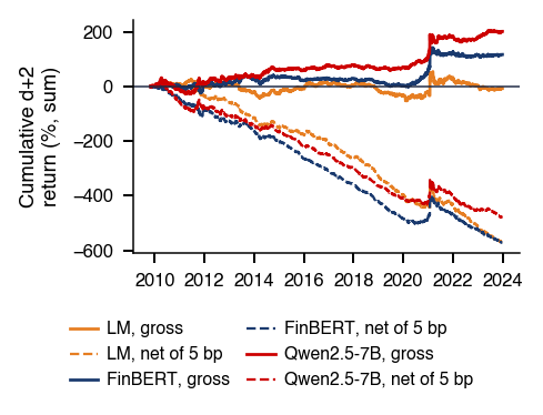
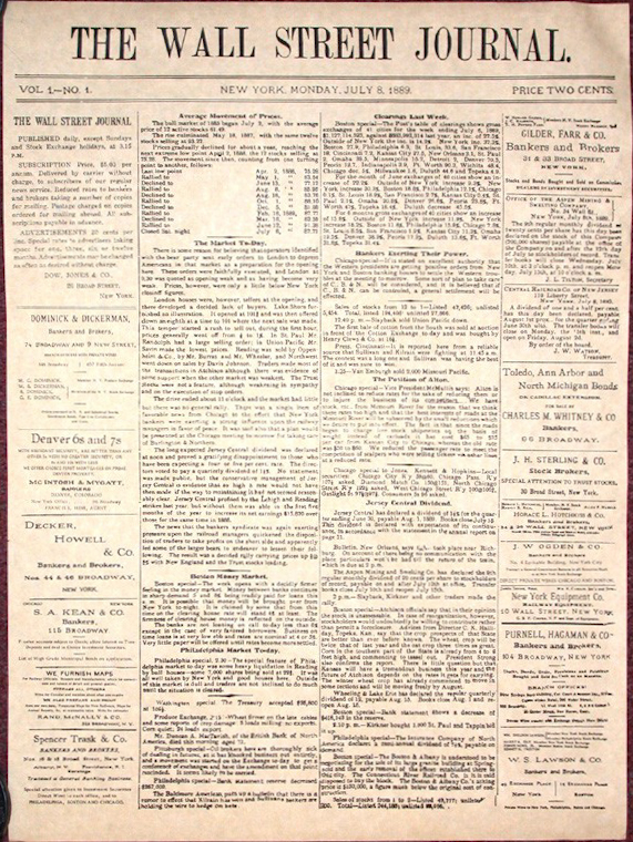

 MFM_ch15_dictionaries