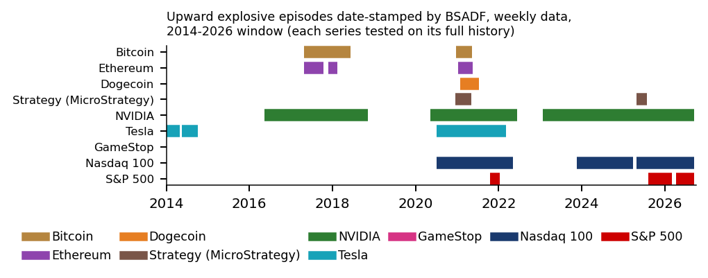
Modelling Financial Markets

Chapter 17: Bubbles and Crashes

Chapter 17: Bubbles and Crashes

Daniel Traian PELE

Bucharest University of Economic Studies
IDA Institute Digital Assets
Blockchain Research Center
AI4EFin Artificial Intelligence for Energy Finance
Romanian Academy, Institute for Economic Forecasting
MSCA Digital Finance

The second theorem of the financial instability hypothesis is that over periods of prolonged prosperity, the economy transits from financial relations that make for a stable system to financial relations that make for an unstable system.

— Minsky (1992), The financial instability hypothesis

Minsky (1992) classifies borrowers by whether their cash flows can service their debt: hedge finance covers interest and principal, speculative finance only the interest, and Ponzi finance not even the interest, so that repayment depends on a rising asset price. A long period of stability shifts the weight of borrowers towards speculative and Ponzi finance. Kindleberger & Aliber (2005) describe the same dynamics as a sequence: displacement, boom, euphoria, distress and panic. The tulip mania, the South Sea and Mississippi bubbles of 1720 and the crash of 1929 show, however, why a bubble is hard to call: to call a price a bubble we need a model of fundamental value, and the test must work on a single time series, in real time, before the panic.

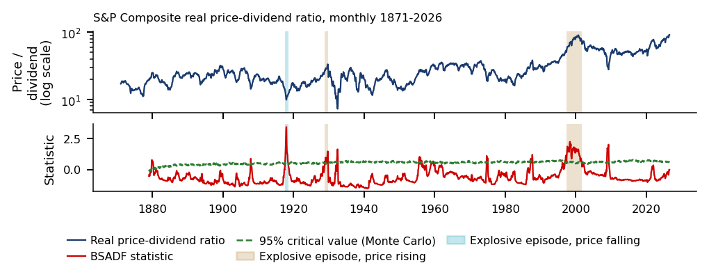
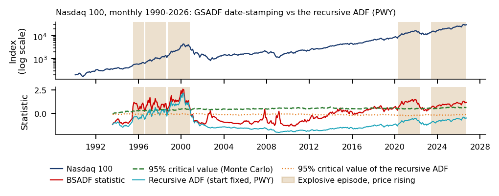
Explosiveness tests answer the second requirement. On the S&P (Standard & Poor's) Composite price-dividend ratio, monthly from 1871 to 2026, the GSADF (Generalised Sup Augmented Dickey–Fuller) statistic of Phillips, Shi & Yu (2015a) is 3.41, against a 95% critical value of 2.39, while the full-sample ADF (Augmented Dickey–Fuller) test, at −1.11, sees nothing. Date-stamping finds the episodes Nov 1928–Sep 1929 and May 1997–Aug 2001. The dot-com peak of the ratio is 90.2, in Aug 2000, against a long-run mean of 29.8, but the sample maximum, 91.2 in May 2026, falls in no episode: a high ratio is not necessarily explosive.

The second question is whether a sharp run-up announces a crash. In the industry data of Greenwood, Shleifer & You (2019), replicated in the course, a run-up above 100% was followed by a 40% crash in 45% of cases, with a 95% confidence interval (CI) of [27%, 62%], against 11% for a random industry-month. The mean return over the next two years, however, is not significantly different from zero, so run-ups raise the risk of a crash, not the predictable loss. The credit that finances the boom, Minsky's mechanism, appears in the study of Greenwood, Hanson, Shleifer & Sørensen (2022): in the course replication, after rapid growth of credit and asset prices (the R-zone), a household-sector crisis begins within three years in 34% of cases, against 4% in normal periods, based on only 25 crises.

S&P Composite (Shiller) price-dividend ratio, monthly, Jan 1871–Jun 2026. Top: the real price divided by the real dividend, on a log scale; bottom: the BSADF statistic and the 95% critical value (Monte Carlo). The shaded areas are the date-stamped explosive episodes: beige when the ratio rises, blue when it falls.
S&P Composite (Shiller) price-dividend ratio, monthly, Jan 1871–Jun 2026. Top: the real price divided by the real dividend, on a log scale; bottom: the BSADF (Backward Sup Augmented Dickey–Fuller, statistic) statistic and the 95% critical value (Monte Carlo). The shaded areas are the date-stamped explosive episodes: beige when the ratio rises, blue when it falls. Interactive chart: “S&P Composite (Shiller) Price-Dividend Ratio, 1871–2026 (1/2)” →

What you will be able to do

  • Derive the rational-bubble condition and separate fundamental value from the bubble, with what can be tested.
  • Compute the GSADF statistic and BSADF (Backward Sup Augmented Dickey–Fuller) date-stamping on rolling windows, with valid critical values.
  • Compute an LPPLS (Log-Periodic Power Law Singularity) fit and interpret the stability of the critical time and its alarms.
  • Interpret run-ups and crashes with a Markov-switching model and the test for the number of regimes.

The Further Topics and the Appendix are reading for familiarity.

Chapter plan

  1. Motivation: Detecting Bubbles in Real TimeThe chapter's question, three historical lessons and Minsky's financial instability hypothesis.
  2. What Is a Bubble?Fundamental value, the rational bubble, bubbles that burst and bubbles beyond rational expectations.
  3. Run-Ups and Crashes in the DataNine episodes aligned at the peak and the crash frequency after sharp run-ups.
  4. Testing for Explosive BehaviourThe right-tailed ADF, recursive windows, date-stamping, critical values and the applications to the S&P and Bitcoin.
  5. The Log-Periodic Power Law (LPPLS)Crashes as critical points, qualified fits and the confidence indicator.
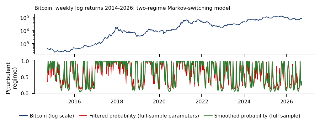
  6. Regime-Switching ModelsThe Markov-switching model on the Nasdaq 100 and the test for the number of regimes.
  7. Crypto and AI BubblesCrypto-assets, the dot-com–AI (Artificial Intelligence) comparison and what the tests can say.
  8. Case Studies: Housing Speculators and Predictable CrisesSpeculators in the US (United States) housing boom and the probability of a crisis after the R-zone.
  9. AI for Scientific DiscoveryOpen questions and the checks needed for a bubble detector.
  10. ConclusionsKey ideas and the practical decision.
  11. Further TopicsDetailed examples and advanced topics.
  12. AppendixThe series tested, derivations and details of the methods.

Motivation: Detecting Bubbles in Real Time

The chapter studies episodes in which a price rises far faster than any plausible change in fundamentals and then loses most of its value. Two questions organise it: whether statistics can detect such an episode in real time, and whether it can say when the episode ends. The first half builds the definition of a bubble and the tests for explosive prices; the second half adds the log-periodic model of crashes, regime switching and two case studies.

The Idea of the Chapter

Slide 2 in the PDF

A bubble is usually recognised after the crash, when the fall makes it plain that the earlier price could not be justified. A statistical answer has to work before that point, on a single price series and with the data available at each date. The chapter therefore asks two separate questions: can a test flag an episode while it is happening, and can any model date its end.

Part I defines a bubble, documents run-ups and crashes in the data and develops the tests for explosive prices with their date-stamping rules. Part II covers the LPPLS (Log-Periodic Power Law Singularity) model, Markov regime switching, the crypto and artificial-intelligence (AI) stocks, two case studies and one pass of the AI-assisted research loop. The Further Topics and the Appendix give detailed examples and derivations.

In brief

Bubbles, Crashes and Their Detection
  • Prices sometimes rise far faster than any plausible change in fundamentals
    • Then they lose most of their value
  • Questions
    • can statistics detect such episodes in real time?
    • can it say when they end?
  • Part I
    • What a bubble is, run-ups and crashes in the data
    • Tests for explosive prices and their date-stamping
  • Part II: the LPPLS model (Log-Periodic Power Law Singularity)
    • Regime switching, crypto and artificial-intelligence (AI) stocks
    • Two case studies, one pass of the AI-assisted research loop
What you should be able to do
  • derive the rational-bubble condition split price into fundamental value and bubble, say what is testable
  • compute GSADF and the BSADF (Backward Sup ADF) date-stamping on rolling windows, with valid critical values
  • compute an LPPLS fit and interpret the stability of its critical time and its alarms
  • interpret booms and busts with a Markov-switching model and the test of the number of regimes
  • Further Topics and Appendix: reading for familiarity
  • Detailed examples, advanced topics: Further Topics, after the Conclusions
    • the footer button leads there: Back returns to the starting slide

Historical Bubble Episodes

Slide 3 in the PDF

Three historical episodes give the requirements a bubble test must meet, one lesson each:

  1. Calling something a bubble requires a model of the fundamental value. In the tulip market of 1636–1637, contracts on rare bulbs traded at very high prices until the market stopped in February 1637 (Garber, 1990), and part of the price path fits the fundamentals of a new luxury good.
  2. Bubbles come with credit expansion (Kindleberger & Aliber, 2005) and with high turnover (Scheinkman & Xiong, 2003). The South Sea and Mississippi episodes of 1720 saw shares rise several-fold within months and then collapse (Kindleberger & Aliber, 2005); their ingredients were a financial innovation, easy credit and a story about future profits.
  3. On method, the tests must work on a single time series, in real time, before the panic. The boom of 1929, partly financed with borrowed money, ended in the October crash; Kindleberger's sequence, which follows Minsky, describes the stages: displacement, boom, euphoria, distress and panic.

In brief

Historical Bubble Episodes Hendrik Gerritsz Pot, Flora's Wagon of Fools (c. 1637), a satire of the tulip trade Image: Hendrik Gerritsz Pot (c. 1637); public domain; Wikimedia Commons
  • Tulips, 1636–1637 Garber (1990)
    • Contracts on rare bulbs traded at very high prices until the market stopped in February 1637
    • Part of the path fits the fundamentals of a new luxury good
    • Lesson 1: calling something a bubble requires a model of the fundamental value
  • South Sea and Mississippi, 1720 Kindleberger & Aliber (2005)
  • 1929 Kindleberger & Aliber (2005)
    • A boom partly financed with borrowed money ended in the October crash
    • Kindleberger's sequence (after Minsky): displacement, boom, euphoria, distress, panic
    • Lesson 3: we need tests that work on a single time series, in real time, before the panic

Case Study: Black Thursday, 24 October 1929 (1/2)

Slide 4 in the PDF

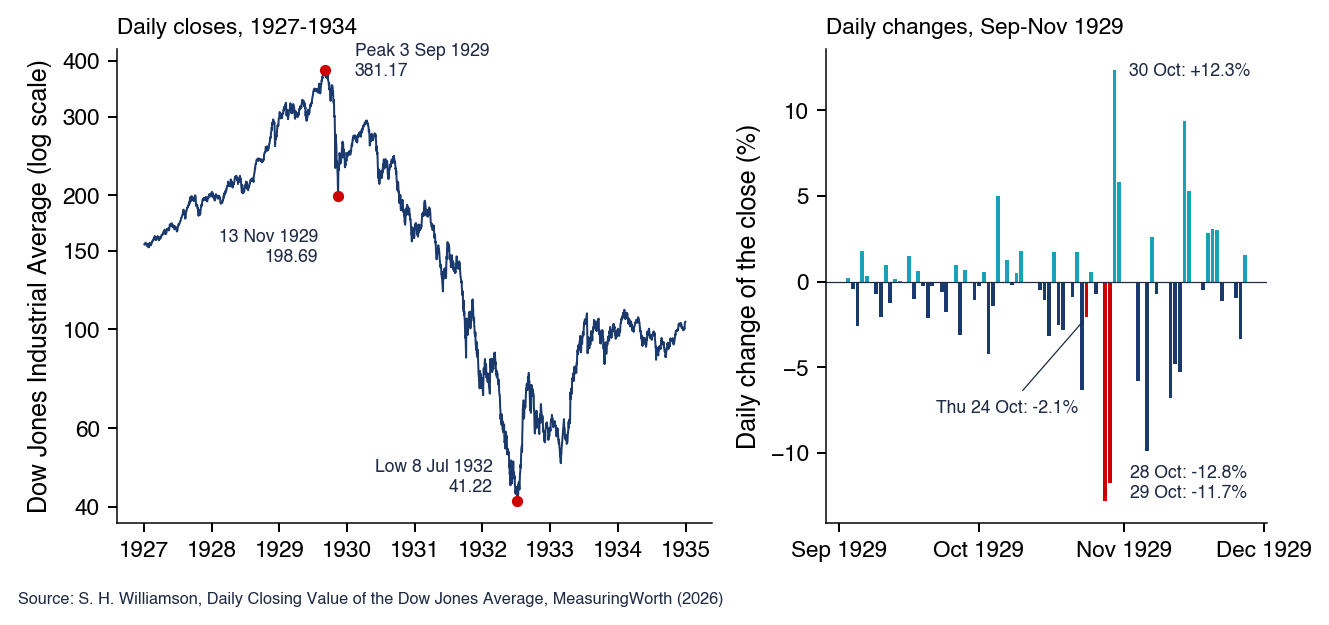
The chart shows the Dow Jones Industrial Average in daily closes, from the series of Williamson (2026). On the left, the index on a log scale, 1927–1934, with the peak of 3 September 1929, the low of 13 November 1929 and the low of 8 July 1932; on the right, the daily changes of September–November 1929, with 24, 28 and 29 October in red.

In brief

Case Study: Black Thursday, 24 October 1929 (1/2)
  • Dow Jones Industrial Average, daily closes, log scale on the left; source: Williamson (2026)
MFM_ch17_case1929

Case Study: Black Thursday, 24 October 1929 (2/2)

Slide 5 in the PDF

The index reached 381.17 on 3 September 1929, after a rise of 99% in two years. The fall had begun before Black Thursday: on 23 October the index closed at 305.85, 20% below the peak, after a fall of 6.3% on that day alone.

On Thursday, 24 October, 12,894,650 shares traded on the New York Stock Exchange (NYSE), a record (Time, 1929). The heads of the large New York banks, called together at J.P. Morgan & Co. by Thomas Lamont, organised a support pool, and Richard Whitney, vice-president of the exchange, bid 205 dollars a share for U.S. Steel, above the current price. The index closed at 299.47, down 2.1%, a smaller fall than on the day before.

The support did not stop the decline. On Monday, 28 October, and Tuesday, 29 October, the index lost 12.8% and 11.7%, the largest daily falls of 1921–1955; on 30 October it rose by 12.3%, and on 13 November it closed at 198.69, 48% below the peak. A rebound of 48% to 17 April 1930 followed, then the low of 41.22 on 8 July 1932, 89% below the peak. The nominal 1929 level was regained only on 23 November 1954. The crash was a sequence of weeks and years, not a single day.

In brief

Case Study: Black Thursday, 24 October 1929 (2/2) The crowd outside the New York Stock Exchange after the crash, October 1929 Photo: US (United States) government (Social Security Administration); public domain; Wikimedia Commons
  • Before: the peak of 381.17 on 3 Sep 1929, after a rise of 99% in two years
    • By 23 Oct the index had already fallen by 20%, to 305.85; on that day alone \(-6.3\%\)
  • Thursday, 24 Oct: 12 894 650 shares traded on the New York Stock Exchange (NYSE), a record Time (1929)
    • Heads of the large New York banks, called together at J.P. Morgan & Co. by Thomas Lamont, organise a support pool
    • Richard Whitney, vice-president of the NYSE, bids 205 dollars a share for U.S. Steel, above the current price
    • Close: 299.47, that is \(-2.1\%\), a smaller fall than on 23 Oct
  • Monday 28 and Tuesday 29 Oct: \(-12.8\%\) and \(-11.7\%\), the largest daily falls of 1921–1955
    • 30 Oct: \(+12.3\%\); 13 Nov: 198.69, 48% below the peak
  • Afterwards: a rebound of 48% to 17 Apr 1930, then the low of 41.22 on 8 Jul 1932 (\(-89\%\))
    • The nominal 1929 peak was regained only on 23 Nov 1954
  • The lesson: the bankers' support stopped one day's panic, not the decline
    • The crash was a sequence of weeks and years, not a single day

The Financial Instability Hypothesis: Minsky

Slide 6 in the PDF

Minsky (1992) classifies borrowers by whether their cash flows can service their debt:

  • Under hedge finance the cash flows cover both interest and principal.
  • Under speculative finance they cover the interest, but the principal must be rolled over.
  • Under Ponzi finance they do not even cover the interest, so the debt grows and repayment depends on rising asset prices.

The fragility mechanism follows from this classification. A long calm period shifts borrowers towards speculative and Ponzi finance. Higher interest rates or falling prices then turn speculative borrowers into Ponzi borrowers, and the forced asset sales that follow push prices down and drive other borrowers towards insolvency.

The hypothesis links to the chapter in two places:

  1. The credit that finances the boom is the subject of the second case study, on crises after rapid growth of credit and asset prices.
  2. The acceleration of prices is what the explosiveness tests measure.

In brief

  • Minsky classifies borrowers by whether their cash flows can service their debt Minsky (1992)
    • Hedge finance: cash flows cover both interest and principal
    • Speculative finance: they cover interest, but the principal must be rolled over
    • Ponzi finance: they do not even cover interest; debt grows and repayment relies on rising asset prices
  • The fragility mechanism
    • A long calm period shifts borrowers towards speculative and Ponzi finance
    • Higher interest rates or falling prices turn speculative borrowers into Ponzi borrowers
    • Forced asset sales push prices down and drive other borrowers towards insolvency
  • The link with this chapter
    • The credit that finances the boom: the second case study
    • Accelerating prices: the explosiveness tests

What Is a Bubble?

A bubble is defined relative to a fundamental value, so the section starts from the no-arbitrage pricing equation and derives the part of the price it does not pin down. The rational bubble that results has an explosive conditional mean, which gives the testable implication used in the rest of the chapter. Models of bubbles that burst and restart, and bubbles driven by beliefs rather than rational expectations, complete the definition.

Fundamental Value and the Rational Bubble

Slide 7 in the PDF

The question is which part of the price cannot be justified by dividends, and what can be tested about it. No-arbitrage pricing states

\[P_t = \mathbb{E}_t\big[M_{t+1}(P_{t+1} + D_{t+1})\big],\]
(17.1)

where \(P_t\) is the price at the end of period \(t\), \(D_{t+1}\) the dividend paid in period \(t+1\), \(M_{t+1}\) the stochastic discount factor and \(\mathbb{E}_t\) the expectation under the physical measure given the information at \(t\).

Under the simplifying assumption \(M_{t+1} \equiv 1/(1+r)\), (17.1) becomes \(P_t = \mathbb{E}_t[P_{t+1} + D_{t+1}]/(1+r)\). A constant risk premium does not make \(M_{t+1}\) constant; in general, the bubble satisfies \(B_t = \mathbb{E}_t[M_{t+1}B_{t+1}]\). Solving forward gives the fundamental value, the present value of expected dividends,

\[F_t = \sum_{i \ge 1} \frac{\mathbb{E}_t[D_{t+i}]}{(1+r)^i},\]
(17.2)

which in the Gordon case of dividends growing at \(g < r\) reduces to \(F_t = D_{t+1}/(r-g)\).

The forward solution is not the only one. The price \(P_t = F_t + B_t\) also solves the pricing equation for any \(B_t\) with

\[\mathbb{E}_t[B_{t+1}] = (1+r)\,B_t.\]
(17.3)

The term \(B_t\) is the rational bubble: investors pay for it because they expect to resell at a higher price (Blanchard & Watson, 1982).

In brief

  • Question: which part of the price cannot be justified by dividends, and what can we test about it?
  • No-arbitrage pricing: \(P_t = \E_t[M_{t+1}(P_{t+1} + D_{t+1})]\)
    • \(P_t\): price at the end of period \(t\); \(D_{t+1}\): dividend paid in period \(t + 1\)
    • \(M_{t+1}\): stochastic discount factor; \(\E_t\): expectation under the physical measure, given the information at \(t\)
  • Simplifying assumption: \(M_{t+1} \equiv 1/(1 + r)\), so \(P_t = \E_t[P_{t+1} + D_{t+1}]/(1 + r)\)
    • A constant risk premium does not make \(M_{t+1}\) constant
    • In general, the bubble satisfies \(B_t = \E_t[M_{t+1}B_{t+1}]\)
  • Solving forward gives the fundamental value \(F_t = \sum_{i \ge 1} \E_t[D_{t+i}]/(1 + r)^i\)
    • The present value of expected dividends
    • Gordon case, dividends growing at \(g < r\): \(F_t = D_{t+1}/(r - g)\)
  • But \(P_t = F_t + B_t\) also solves the pricing equation, for any \(B_t\) with \(\E_t[B_{t+1}] = (1 + r)\,B_t\)
    • \(B_t\) is the rational bubble: investors pay for it because they expect to resell at a higher price Blanchard & Watson (1982)

Why a Rational Bubble Must Explode

Slide 8 in the PDF

Iterating (17.3) gives \(\mathbb{E}_t[B_{t+h}] = (1+r)^h B_t\) for any horizon of \(h\) periods. The bubble has an explosive conditional mean, although individual paths can crash. Because it grows at the rate \(r\), faster than dividends (\(r > g\)), its share of the price rises over time.

Diba & Grossman (1988) show further restrictions. A negative bubble would eventually push the expected price below zero, so rational bubbles are positive. A bubble that is zero today must stay zero, so a rational bubble exists from the first trade. Equivalently, a bubble is the failure of the transversality condition \(\lim_{h\to\infty}\mathbb{E}_t[P_{t+h}]/(1+r)^h = 0\): the price contains a value that is never paid out as dividends. The derivation is in the Appendix.

The testable implication is the basis of the chapter's tests. If dividends are at most integrated of order one, I(1), then without a bubble neither the price nor the price-dividend ratio is explosive. An explosive root in either is evidence against the no-bubble model, given the assumption on dividends.

In brief

  • From \(\E_t[B_{t+1}] = (1 + r)B_t\): \(\E_t[B_{t+h}] = (1 + r)^h B_t\) for any horizon of \(h\) periods
    • An explosive conditional mean
    • Individual paths can crash
    • The bubble grows faster than dividends (\(r > g\)), so its share of the price rises over time
  • Rational bubbles are positive and exist from the first trade Diba & Grossman (1988)
    • A negative bubble would eventually push the expected price below zero
    • A bubble that is zero today must stay zero
  • A bubble is the failure of the transversality condition \(\lim_{h \to \infty} \E_t[P_{t+h}]/(1 + r)^h = 0\)
    • The price contains a value never paid out as dividends (derivation in the Appendix)
  • Testable implication
    • If dividends are at most I(1) (stationary after one differencing), then without a bubble the price and the price-dividend ratio are not explosive

Bubbles That Burst: Blanchard and Watson

Slide 9 in the PDF

A rational bubble need not grow forever. In the model of Blanchard & Watson (1982) the bubble survives each period with probability \(\pi\) and collapses with probability \(1-\pi\):

\[B_{t+1} = \begin{cases} \dfrac{1+r}{\pi}\,B_t + \varepsilon_{t+1} & \text{with probability } \pi,\\[4pt] \varepsilon_{t+1} & \text{with probability } 1-\pi, \end{cases}\]
(17.4)

where \(\pi \in (0,1)\) and \(\varepsilon_{t+1}\) is a shock with mean zero given the information at \(t\).

The expected growth of the bubble in (17.4) is still \(r\), so the condition (17.3) holds. While it survives, however, the bubble grows faster, at the rate \((1+r)/\pi - 1\), which compensates the holder for the risk of collapse. The waiting time until the collapse is geometric, with expected lifetime \(1/(1-\pi)\) periods.

In brief

  • Each period the bubble survives with probability \(\pi\) and collapses with probability \(1 - \pi\) Blanchard & Watson (1982)
    • \(B_{t+1} = \dfrac{1 + r}{\pi}\,B_t + \varepsilon_{t+1}\) with probability \(\pi\), \(\ B_{t+1} = \varepsilon_{t+1}\) otherwise
    • \(\pi \in (0, 1)\): survival probability; \(\varepsilon_{t+1}\): a shock with mean zero given the information at \(t\)
  • Expected growth is still \(r\)
    • While it survives the bubble grows faster, at \((1 + r)/\pi - 1\), to pay for the crash risk
  • Expected lifetime: \(1/(1 - \pi)\) periods, a geometric waiting time

The Evans Form: Bubbles That Restart

Slide 10 in the PDF

After a Blanchard–Watson collapse the bubble equals the shock \(\varepsilon\), which can be negative, and negative bubbles are ruled out by Diba & Grossman (1988). In the form of Evans (1991) the bubble starts and restarts from a value \(\delta > 0\). If \(B_t > \alpha\), it survives with probability \(\pi\) as \(B_{t+1} = [\delta + \frac{1+r}{\pi}(B_t - \frac{\delta}{1+r})]u_{t+1}\) and collapses with probability \(1-\pi\) to \(B_{t+1} = \delta\,u_{t+1}\), where \(u_{t+1}\) is positive noise with mean 1 drawn independently of survival.

The bubble condition still holds: \(\mathbb{E}_t[B_{t+1}] = \pi[\delta + \frac{1+r}{\pi}B_t - \frac{\delta}{\pi}] + (1-\pi)\delta = (1+r)B_t\). Below the threshold, for \(B_t \le \alpha\), the small-bubble branch \(B_{t+1} = (1+r)B_t u_{t+1}\) applies. The threshold is needed because the survival branch turns negative for \(B_t < \delta(1-\pi)/(1+r)\); with \(0 < \delta < (1+r)\alpha\) the bubble stays positive. The simulation of the next slides uses \(\alpha = \delta\).

In brief

  • The problem: after a Blanchard–Watson collapse, \(B = \varepsilon\) can be negative, which Diba & Grossman (1988) rule out
  • Evans form: the bubble starts and restarts from a value \(\delta > 0\) Evans (1991)
    • Survival (probability \(\pi\)): \(B_{t+1} = \big[\delta + \frac{1 + r}{\pi}(B_t - \frac{\delta}{1 + r})\big]u_{t+1}\)
    • Collapse (probability \(1 - \pi\)): \(B_{t+1} = \delta\,u_{t+1}\)
    • \(u_{t+1}\): positive noise with mean 1, drawn independently of survival
  • The bubble condition still holds: \(\E_t[B_{t+1}] = \pi\big[\delta + \frac{1 + r}{\pi}B_t - \frac{\delta}{\pi}\big] + (1 - \pi)\delta = (1 + r)B_t\)
  • Small-bubble branch: if \(B_t \le \alpha\), then \(B_{t+1} = (1 + r)B_t u_{t+1}\)
    • The two branches above apply only for \(B_t > \alpha\)
    • Without the threshold, the survival branch turns negative for \(B_t < \delta(1 - \pi)/(1 + r)\)
    • With \(0 < \delta < (1 + r)\alpha\) the bubble stays positive; the simulation uses \(\alpha = \delta\)

A Simulated Rational Bubble (1/2)

Slide 11 in the PDF
    Question for the room For an Evans bubble much larger than its restart value δ, with r = 1%, how does the mean growth rate conditional on survival change when ▶ raises π from 0.97 to 0.995?
    Answer

    It falls from about 4.1% to 1.5% per period. For Bₜ > δ, the mean growth rate conditional on survival is (1 + r)/π − 1 − (δ/Bₜ)(1 − π)/π; when Bₜ is much larger than δ, the last term is small. The unconditional mean growth stays at r = 1%; it is not the growth rate conditional on survival. The values 33.3 and 200 periods, 1/(1 − π), are geometric waiting times under a constant collapse risk, not the exact duration of Evans episodes. With π = 0.97, the simulated bubble collapsed visibly 4 times, and at its peak the price was 1.46 times the fundamental value.

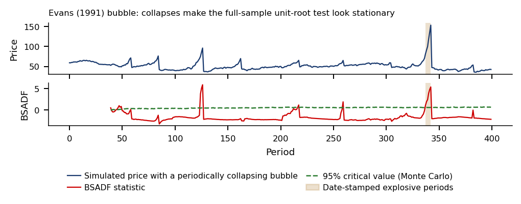
    The chart shows one simulated path of an Evans bubble added to the fundamental value of a stock with random-walk dividends. The price \(P_t = F_t + B_t\) is in blue and the fundamental value \(F_t\) in green, over 400 periods; the parameters are on the next slide.

    A Simulated Rational Bubble (2/2)

    Slide 12 in the PDF

    Dividends \(D_t\) follow a random walk, the discount rate is \(r = 1\%\), the survival probability \(\pi = 0.97\), and the Evans parameters are \(\delta = \alpha = 5\). Since \(\mathbb{E}_t[D_{t+i}] = D_t\), the fundamental value (17.2) is \(F_t = \sum_{i\ge1} D_t/(1+r)^i = D_t/r\). While it is alive and large, the bubble grows by \((1+r)/\pi - 1 \approx 4.1\%\) per period.

    On the simulated path the bubble grew large and burst 4 times, and at its largest the price was 1.46 times the fundamental value. Between episodes the price tracks fundamentals. A test on the full sample therefore sees mostly normal data, which is why the tests of this chapter are run on windows.

    In brief

    • Simulation
      • Random-walk dividends \(D_t\)
      • Discount rate \(r = 1\%\), survival probability \(\pi = 0.97\)
      • Evans form with \(\delta = \alpha = 5\)
      • Fundamental value: \(\E_t[D_{t+i}] = D_t\), so \(F_t = \sum_{i \ge 1} D_t/(1 + r)^i = D_t/r\)
      • While alive and large, the bubble grows by \((1 + r)/\pi - 1 \approx 4.1\%\) per period
    • The chart: price \(P_t = F_t + B_t\) (blue) and fundamental value \(F_t\) (green), over 400 periods
    • The bubble grew large and burst 4 times
      • At its largest the price was \(1.46\) times the fundamental value
    • Between episodes the price tracks fundamentals
      • A full-sample test sees mostly “normal” data: the tests of this chapter use windows
    MFM_ch17_rational_bubble

    Bubbles Beyond Rational Expectations

    Slide 13 in the PDF

    Rational bubbles are not the only explanation of prices that run ahead of fundamentals:

    • Shiller (2015) stresses feedback and narratives: rising prices attract new buyers, and "new era" stories spread by word of mouth.
    • In the model of Scheinkman & Xiong (2003), disagreement among investors combined with short-sale limits makes the price include the option to resell to a more optimistic buyer.
    • Riding the bubble: informed traders stay in as long as others do, since no single trader can burst the bubble alone; the mechanism is modelled by Abreu & Brunnermeier (2003) and documented for hedge funds in the technology bubble by Brunnermeier & Nagel (2004).

    The three explanations share one empirical signature: for a while, prices grow faster than fundamentals. This explosive pattern is what the tests of the chapter look for.

    In brief

    • Feedback and narratives Shiller (2015)
      • Rising prices attract new buyers
      • “New era” stories spread by word of mouth
    • Disagreement and short-sale limits Scheinkman & Xiong (2003)
      • The price includes the option to resell to a more optimistic buyer
    • Riding the bubble Abreu & Brunnermeier (2003), Brunnermeier & Nagel (2004)
      • Informed traders stay in as long as others do, since no one can burst it alone
    • Common signature of all three
      • Prices grow faster than fundamentals for a while: the explosive pattern we will test

    Section summary

    A bubble is the part of the price that the dividends do not justify. Under rational expectations it must have an explosive conditional mean, may burst and restart, and leaves the price or the price-dividend ratio explosive. Behavioural explanations lead to the same signature, so the tests target explosiveness rather than a particular mechanism.

    Run-Ups and Crashes in the Data

    Before the formal tests, the section looks at what famous bubbles have in common and at the systematic evidence on whether sharp run-ups are followed by crashes. The famous episodes are selected on the outcome, so the evidence that matters comes from all industries rather than from a list of crashes.

    Nine Episodes: Run-Up and Crash

    Slide 14 in the PDF

    The table lists nine episodes from equity indices, single stocks and cryptos. For each, the peak is the highest daily close of the episode, the run-up is the simple percentage change of the price over the two years before the peak, \(P_{\text{peak}}/P_{\text{peak}-2\text{y}} - 1\), and the maximum fall is measured to the lowest close within four years. The last column gives the month when the price was back at the peak.

    The run-ups range from +97% for the BET (Bucharest Exchange Trading, index) index before July 2007 to +124,004% for Ethereum before January 2018, while the falls lie between −74% (Tesla, 2021) and −94% (Ethereum, 2018). The BET episode of 2007 is the only one without a spectacular run-up in the last two years, yet its fall, −83%, is among the deepest. Dogecoin and GameStop had not regained their 2021 peaks by the end of the sample.

    In brief

    • Question: are very fast run-ups followed by crashes, and how often?
    EpisodePeak2-year run-upMax. fallTroughBack at peak
    Nasdaq 100, 200027 Mar 2000\(+288\%\)\(-83\%\)Oct 2002Nov 2015
    Cisco, 200027 Mar 2000\(+592\%\)\(-89\%\)Oct 2002Aug 2021
    BET, 200724 Jul 2007\(+97\%\)\(-83\%\)Feb 2009Mar 2021
    Bitcoin, 201716 Dec 2017\(+4\,186\%\)\(-83\%\)Dec 2018Nov 2020
    Ethereum, 201813 Jan 2018\(+124\,004\%\)\(-94\%\)Dec 2018Feb 2021
    Bitcoin, 20218 Nov 2021\(+667\%\)\(-77\%\)Nov 2022Mar 2024
    Dogecoin, 20217 May 2021\(+26\,897\%\)\(-92\%\)Jun 2022not yet
    GameStop, 202127 Jan 2021\(+2\,218\%\)\(-88\%\)Apr 2024not yet
    Tesla, 20214 Nov 2021\(+1\,837\%\)\(-74\%\)Jan 2023Dec 2024
    • Peak: highest daily close in the episode
    • Run-up: simple percentage change of the price over the two years before the peak
      • \(P_{\text{peak}}/P_{\text{peak} - 2\text{y}} - 1\)
    • Maximum fall: to the lowest close within four years
    • BET 2007 (Bucharest Exchange Trading, index): the only episode without a spectacular run-up in the last two years
      • Yet with one of the deepest falls

    Run-Ups and Crashes Aligned at the Peak (1/2)

    Slide 15 in the PDF
      Question for the room All nine selected episodes were followed by crashes. Can we use the proportion 9/9 to estimate the probability of a crash after a rapid run-up?
      Answer

      No. Selecting on the outcome excludes run-ups that did not end in a crash, and removing an extreme episode does not repair this selection. The run-ups over the two years before the peak range from +97% (BET, 2007) to +124,004% (Ethereum, 2018). The chart shows the maximum fall in the first two years after the peak, between −74% (Tesla) and −94% (Ethereum); the lecture table uses four years. For the Nasdaq 100, these are −76% and −83% respectively.

      The chart aligns the nine episodes at their peaks. Each line shows daily prices from two years before to two years after the peak, normalised to 100 at the peak and plotted on a log scale.

      Run-Ups and Crashes Aligned at the Peak (2/2)

      Slide 16 in the PDF

      The two-year run-ups differ by orders of magnitude, while the falls are much closer, between 74% and 94%. The common shape is an accelerating rise, a sharp top and a deep fall. On the log scale the rise is convex: the growth rate itself increases, which is the explosive behaviour the tests look for.

      The picture has a selection bias. The episodes were picked because they crashed, and many run-ups were not followed by crashes. Whether a sharp run-up predicts a crash has to be measured on a sample that is not selected on the outcome, which is the design of the next slides.

      In brief

      • Daily prices two years before and after each peak, peak = 100, log scale
      • Two-year run-ups differ by orders of magnitude, the falls much less (\(74\)–\(94\%\))
      • Common shape: an accelerating rise, a sharp top, a deep fall
        • Convex on the log scale: the growth rate itself rises, the explosive behaviour the tests look for
      • Selection bias: we picked these episodes because they crashed
        • Many run-ups were not followed by crashes
      MFM_ch17_episodes

      Bubbles for Fama: The Design

      Slide 17 in the PDF

      Fama (2014) objects that a "bubble" is only a bubble if its end is predictable; otherwise the run-up may be a rational reaction to news. Greenwood, Shleifer & You (2019) answer with all US industries since 1926, not with famous episodes only, and ask whether sharp run-ups predict crashes or low returns.

      A run-up is defined by the value-weighted industry return over the past two years, with each firm weighted by its market capitalisation. Both the raw return and the return net of the market must exceed a threshold, for example 100%, and the raw return over the past five years must be at least 50% (from 1931), so that recoveries from slumps are not counted. The episode is dated at the first month of the run-up, and a new episode in the same industry is counted only two years later.

      A crash is a drawdown of at least 40% from a previous high within the next two years. Each crash frequency comes with a 95% confidence interval (CI). The sample is the first 48 of the 49 industries of the Kenneth French data library, without "Other", restricted to months with at least ten firms: 41,721 industry-months, 1926–2026.

      In brief

      • Fama's objection: a “bubble” is only a bubble if its end is predictable Fama (2014)
        • Otherwise it may be a rational reaction to news
      • Greenwood, Shleifer and You answer with all US industries since 1926 Greenwood, Shleifer & You (2019)
        • Not with famous episodes only
        • Do sharp run-ups predict crashes, or low returns?
      • Run-up: value-weighted industry return over the past 2 years above a threshold (e.g. \(100\%\))
        • Each firm weighted by its market capitalisation
        • Both conditions at once: the raw return and the return net of the market exceed the threshold
        • And a raw return of at least \(50\%\) over the past 5 years (from 1931), so that recoveries from slumps are not counted
        • First month of the run-up; a new episode in the same industry only two years later
      • Crash
        • A drawdown of at least \(40\%\) from a previous high within the next 2 years
        • Each crash frequency comes with a 95% CI (Confidence Interval)
      • The sample: the first 48 of the 49 industries of the Kenneth French Data Library (without “Other”)
        • Months with at least ten firms: 41 721 industry-months, 1926–2026

      What Do Sharp Run-Ups Predict? (1/2)

      Slide 18 in the PDF
        Question for the room Among the 53 episodes selected by the Greenwood, Shleifer and You rule, a crash of at least 40% follows in 45% of the cases. The mean return over the next two years is +2%, with a 95% CI of [−13%, 20%]. Which conclusion about the mean return do the data support?
        Answer

        There is no clear evidence that it is negative. The frequency of a crash and the return at the end of the two years measure different things. The interval contains negative and positive values; it does not establish that the mean is zero. A crash follows in 45% of the cases (53 episodes in 27 industries, 95% CI [27%, 62%]), against 11% for an arbitrary industry-month. Selection requires the two-year return to exceed the threshold both raw and in excess of the market, a raw five-year return of at least 50%, and at least two years between episodes of the same industry.

        The left panel shows the crash frequency after run-ups above each threshold, with its 95% CI, and the right panel the mean two-year return after the run-up. The dashed line gives the same quantities for all industry-months. The estimator and the reading follow on the next slide.

        What Do Sharp Run-Ups Predict? (2/2)

        Slide 19 in the PDF

        The crash frequency above a threshold \(c\) is

        \[\hat p(c) = \frac{n_{\text{crash}}(c)}{n(c)},\]
        (17.5)

        the share of run-ups above \(c\) followed by a 40% crash, evaluated at the thresholds 50, 75, 100, 125 and 150%. After a run-up above 100%, a crash followed in 45% of cases, from 53 episodes in 27 industries, with a 95% CI of [27%, 62%], against 11% for a random industry-month. Above 150%, the frequency is 71%, from \(n = 21\) episodes.

        The confidence intervals come from a bootstrap over calendar years, because run-ups cluster in time, for example in 1928–1929, 1967–1968 and 1980. The effective sample size is about 31 independent observations (Appendix), well below the 53 episodes.

        The mean return over the next two years is not significantly different from zero: 2% after a 100% run-up, with a CI of [−13%, 20%]. Run-ups raise the risk of a crash, not the predictable loss (Greenwood, Shleifer & You, 2019), and the result does not establish the profitability of a market-timing strategy. What it supports is an association: a conditional frequency in which the run-up precedes the crash, with no mechanism identified.

        In brief

        • Crash frequency above threshold \(c\): \(\hat p(c) = n_{\text{crash}}(c)/n(c)\)
          • The share of run-ups above \(c\) followed by a \(40\%\) crash
          • The chart: left, \(\hat p(c)\) with its 95% CI at the thresholds \(50\), \(75\), \(100\), \(125\) and \(150\%\); right, the mean 2-year return; dashed line: all industry-months
        • After a run-up above \(100\%\), a \(40\%\) crash followed in \(45\%\) of cases
          • 53 episodes in 27 industries
          • 95% CI \([27\%, 62\%]\)
          • Against \(11\%\) for a random industry-month
          • Above \(150\%\): \(71\%\) (\(n = 21\))
        • CI: bootstrap over calendar years, because run-ups cluster in time
          • E.g. 1928–1929, 1967–1968, 1980
          • Effective sample size: about 31 independent observations (Appendix)
        • The mean return over the next 2 years is not significantly different from zero
          • \(2\%\) after a \(100\%\) run-up, CI \([-13\%, 20\%]\)
        • Run-ups raise the risk of a crash, not the predictable loss Greenwood, Shleifer & You (2019)
          • The result does not establish the profitability of a market-timing strategy
        • Type of evidence: association (the variables move together; this does not prove causation)
          • a conditional frequency: the run-up precedes the crash, with no mechanism identified
        MFM_ch17_bubbles_for_fama

        Testing for Explosive Behaviour

        The rational-bubble model implies an explosive root in the price, and the episodes of the previous section show accelerating growth followed by collapse. This section turns the implication into tests on a single series. It starts from the right-tailed Dickey–Fuller regression, extends it to recursive windows, defines the date-stamping rules and their critical values, and then applies them to the S&P price-dividend ratio and to Bitcoin, with checks for changing volatility, serial dependence and multiple testing.

        Right-Tailed ADF (1/2): Regression and Hypothesis

        Slide 20 in the PDF

        The question is how to show, on a single price series, that there was an explosive phase and when it started. The building block is the regression of the change of the log price \(y_t\) on its lagged level,

        \[\Delta y_t = a + b\,y_{t-1} + \varepsilon_t,\]
        (17.6)

        where \(\Delta y_t = y_t - y_{t-1} = \ln(P_t/P_{t-1})\) is the log return and \(\varepsilon_t\) a shock; the chapter's version has no lagged \(\Delta y\) terms. The statistic is \(\mathrm{ADF} = \hat b/\mathrm{SE}(\hat b)\), the Augmented Dickey–Fuller (ADF) \(t\)-statistic, with \(\hat b\) the ordinary least squares (OLS) estimate and SE its standard error.

        The sign of \(b\) classifies the dynamics: \(b < 0\) is mean reversion, \(b = 0\) a random walk (unit root), and \(b > 0\) an explosive path in which each rise feeds the next. The bubble test is \(H_0: b = 0\) against \(H_1: b > 0\), a test in the right tail (Phillips, Wu & Yu, 2011). The usual left-tail Dickey–Fuller table, built for stationary alternatives, does not apply.

        In brief

        • Question: how do we show, on a single price series, that there was an explosive phase and when it started?
        • Regression on the log price \(y_t\): \(\Delta y_t = a + b\,y_{t-1} + \varepsilon_t\)
          • \(\Delta y_t = y_t - y_{t-1} = \ln(P_t/P_{t-1})\): the log return; \(\varepsilon_t\): shock; here no lagged \(\Delta y\)
          • \(\mathrm{ADF} = \hat b / \mathrm{SE}(\hat b)\): the Augmented Dickey–Fuller (ADF) \(t\)-statistic; \(\hat b\): the OLS (Ordinary Least Squares) estimate; SE: its Standard Error
          • \(b < 0\): mean reversion; \(b = 0\): random walk (unit root); \(b > 0\): each rise feeds the next, an explosive path
        • Bubble test: \(H_0: b = 0\) (unit root) vs \(H_1: b > 0\) (explosive root), the right tail Phillips, Wu & Yu (2011)
          • The left-tail Dickey–Fuller table does not apply

        Right-Tailed ADF (2/2): Collapsing Bubbles

        Slide 21 in the PDF

        A single regression on the full sample has low power against bubbles that collapse periodically (Evans, 1991). After repeated collapses the whole series looks stationary or like a random walk, and the collapses give the full-sample slope \(\hat b\) a negative sign (Appendix).

        The solution is to run the regression (17.6) on many windows and take the largest statistic. The SADF (Sup Augmented Dickey–Fuller) test of Phillips, Wu & Yu (2011) and the GSADF (Generalised SADF) test of Phillips, Shi & Yu (2015a) differ in the set of windows they search.

        In brief

        • Evans: a bubble that collapses periodically leaves the full-sample test with low power Evans (1991)
          • The whole series looks stationary or like a random walk
          • Collapses give the full-sample slope a negative sign (Appendix)
        • Solution: run the ADF regression on many windows and take the largest statistic

        Three Ways to Choose Windows (1/2)

        Slide 22 in the PDF
          Question for the room With T = 440 months, how many ADF regressions does GSADF run with the minimum window of the PSY (Phillips–Shi–Yu, bubble test and date-stamping procedure) rule?
          Answer

          The rule gives r₀ = 0.01 + 1.8/√440 = 0.096, i.e. w₀ = 42 months. SADF runs 399 windows (one per end point), GSADF 79,800 (all start–end pairs), hence the supremum over about 80,000 windows.

          Let \(\mathrm{ADF}_{r_1}^{r_2}\) denote the ADF statistic on the window from fraction \(r_1\) to fraction \(r_2\) of the sample; each bar in the chart is one such regression. The parameter \(r_0\) is the minimum window, as a fraction of the \(T\) changes \(\Delta y_t\), and \(\sup\) is the largest value over the admissible windows. Phillips, Shi & Yu (2015a) recommend

          \[r_0 = 0.01 + 1.8/\sqrt{T},\]
          (17.7)

          so that, for \(T = 440\) months, \(r_0 = 0.096\), i.e. 42 months.

          The choice trades off two errors. Too short a window gives an imprecise ADF statistic and more false alarms; too long a window misses short bubbles. In observations, the minimum window is \(w_0 = r_0T = 0.01T + 1.8\sqrt{T}\): the share \(r_0\) falls towards 1% as \(T\) grows, but the number of observations grows. An episode of fixed length can therefore become too short for the minimum window of a very long sample.

          In brief

          • \(\mathrm{ADF}_{r_1}^{r_2}\): the ADF statistic on the window from fraction \(r_1\) to fraction \(r_2\) of the sample
            • Each bar in the chart is one ADF regression
            • \(r_0\): the minimum window, as a fraction of the \(T\) changes \(\Delta y_t\); \(\sup\): the largest value over the windows allowed
          • Minimum window rule: \(r_0 = 0.01 + 1.8/\sqrt{T}\) Phillips, Shi & Yu (2015a)
            • E.g. \(T = 440\) months: \(r_0 = 0.096\), i.e. 42 months
            • Too short a window: an imprecise ADF and more false alarms; too long: short bubbles are missed
            • \(w_0 = r_0 T = 0.01T + 1.8\sqrt{T}\): the minimum share \(r_0\) falls towards \(1\%\), but the minimum number of observations grows
            • An episode of fixed length can become too short for the minimum window of a very long sample
          MFM_ch17_windows

          Three Ways to Choose Windows (2/2)

          Slide 23 in the PDF

          The three statistics differ in the windows they allow. The SADF statistic of Phillips, Wu & Yu (2011) fixes the start at the first observation and lets the end vary:

          \[\mathrm{SADF}(r_0) = \sup_{r_2 \in [r_0,1]} \mathrm{ADF}_0^{r_2}.\]

          The GSADF statistic of Phillips, Shi & Yu (2015a) lets both ends vary, subject to a length of at least \(r_0\):

          \[\mathrm{GSADF}(r_0) = \sup_{r_2 \in [r_0,1]}\ \sup_{r_1 \in [0,\,r_2-r_0]} \mathrm{ADF}_{r_1}^{r_2}.\]
          (17.8)

          The BSADF (Backward SADF) statistic fixes the end point \(r_2\) and searches backwards over the start, \(\mathrm{BSADF}_{r_2} = \sup_{r_1 \in [0,\,r_2-r_0]} \mathrm{ADF}_{r_1}^{r_2}\), so that \(\mathrm{GSADF} = \sup_{r_2}\mathrm{BSADF}_{r_2}\). Because \(\mathrm{BSADF}_{r_2}\) uses only data up to \(r_2\), it can be computed in real time. A larger search needs a higher bar: the critical value is simulated for each \(T\), \(r_0\) and lag order.

          In brief

          • SADF Phillips, Wu & Yu (2011)
            • \(\mathrm{SADF}(r_0) = \sup_{r_2 \in [r_0, 1]} \mathrm{ADF}_0^{r_2}\)
            • Windows start at the first observation and end anywhere after \(r_0\)
          • GSADF Phillips, Shi & Yu (2015a)
            • \(\mathrm{GSADF}(r_0) = \sup_{r_2 \in [r_0, 1]}\ \sup_{r_1 \in [0, r_2 - r_0]} \mathrm{ADF}_{r_1}^{r_2}\)
            • Windows start and end anywhere, with length at least \(r_0\)
          • BSADF (Backward Sup Augmented Dickey–Fuller): backward SADF at the end point \(r_2\) Phillips, Shi & Yu (2015a)
            • \(\mathrm{BSADF}_{r_2} = \sup_{r_1 \in [0, r_2 - r_0]} \mathrm{ADF}_{r_1}^{r_2}\), \(\ \mathrm{GSADF} = \sup_{r_2} \mathrm{BSADF}_{r_2}\)
            • \(\mathrm{BSADF}_{r_2}\) uses only data up to \(r_2\): it can be computed in real time
          • A larger search needs a higher bar: the critical value is simulated for each \(T\), \(r_0\) and lag order

          Date-Stamping an Episode (1/2): the PSY Rules

          Slide 24 in the PDF

          The PSY (Phillips, Shi and Yu) procedure dates the origination of an episode at the first date at which \(\mathrm{BSADF}_{r_2}\) exceeds its critical value \(cv_{r_2}\), the 95% quantile of \(\mathrm{BSADF}_{r_2}\) under the null, computed date by date (Phillips, Shi & Yu, 2015a).

          The termination date (PSY, eq. 8) is the first date after \(\hat r_e + \delta\ln(T)/T\) at which BSADF falls below \(cv_{r_2}\), where \(\hat r_e\) is the estimated start as a fraction of the sample and \(T\) the number of changes \(\Delta y_t\). The term \(\delta\ln(T)/T\) imposes a minimum duration, with \(\delta\) chosen for the data frequency. An isolated exceedance often occurs by chance, and a duration that grows slowly with \(T\) removes short alarms without losing long bubbles.

          The earlier PWY (Phillips, Wu and Yu) date-stamping uses the recursive statistic \(\mathrm{ADF}_0^{r_2}\) instead (Phillips, Wu & Yu, 2011). Because its windows always start at the first observation, it may miss a second bubble after a collapse.

          In brief

          • Origination, in the PSY (Phillips, Shi and Yu) procedure Phillips, Shi & Yu (2015a)
            • The first date at which \(\mathrm{BSADF}_{r_2}\) exceeds its critical value \(cv_{r_2}\)
            • \(cv_{r_2}\): the 95% quantile of \(\mathrm{BSADF}_{r_2}\) under the null, date by date
          • Termination (PSY, eq. 8) Phillips, Shi & Yu (2015a)
            • The first date after \(\hat r_e + \delta \ln(T)/T\) at which \(\mathrm{BSADF}\) falls below \(cv_{r_2}\)
            • \(\hat r_e\): the estimated start, as a fraction of the sample; \(T\): number of changes \(\Delta y_t\)
            • \(\delta \ln(T)/T\): a minimum duration, with \(\delta\) chosen for the data frequency (not the \(\delta\) of the Evans form)
            • Why \(\ln T\): an isolated exceedance often occurs by chance; a duration that grows slowly with \(T\) removes short alarms without losing long bubbles
          • PWY (Phillips, Wu and Yu) date-stamping uses the recursive \(\mathrm{ADF}_0^{r_2}\) instead Phillips, Wu & Yu (2011)
            • It may miss a second bubble after a collapse

          Date-Stamping an Episode (2/2): Minimum Duration, Real Time and Chains

          Slide 25 in the PDF

          The chapter applies the minimum-duration rule of the R package exuber (Vasilopoulos, Pavlidis & Martínez-García, 2022). Runs of consecutive exceedances shorter than \(L = \lceil \ln T \rceil\) periods are dropped, which corresponds to \(\delta = 1\), with \(\lceil\cdot\rceil\) rounding up; \(T = 440\) months gives \(L = 7\). The episode starts at the first exceedance and ends at the last. The PSY rule (eq. 8) would instead turn a single exceedance into an episode of \(L\) periods.

          In real time an episode is confirmed only after \(L\) consecutive exceedances, that is \(L-1\) periods after its start, which is dated in hindsight. Kept runs separated by a short gap form a chain. For monthly data, the next run starts at most 93 days after the previous one ends, at most two months without an exceedance.

          In brief

          • Minimum-duration rule of the R package exuber Vasilopoulos, Pavlidis & Martínez-García (2022)
            • Runs of consecutive exceedances shorter than \(L\) periods are dropped
            • \(L = \lceil \ln T \rceil\), i.e. \(\delta = 1\); \(\lceil \cdot \rceil\): rounded up; \(T = 440\) months gives \(L = 7\)
          • Start: the first exceedance; end: the last exceedance
            • The PSY rule (eq. 8) would turn a single exceedance into an episode of \(L\) periods
          • Real time: the episode is confirmed only after \(L\) consecutive exceedances
            • \(L - 1\) periods after its start, which is dated in hindsight
          • Chain: kept runs separated by a short gap
            • Monthly data: the next run starts at most 93 days after the previous one ends (at most two months without an exceedance)

          Null Distributions and Critical Values (1/2)

          Slide 26 in the PDF
            Question for the room With a minimum window w₀ = 42 months, the 95% critical value of GSADF is 2.19, against −0.06 for a single ADF. ▶ raises w₀ to 132 months. What happens to the GSADF critical value?
            Answer

            It falls to 1.65. GSADF is the maximum of about 80,000 ADF statistics on overlapping windows, and under the null the maximum of many statistics typically exceeds each of them. With a longer minimum window there are fewer windows and the critical value falls (1.65 for w₀ = 132); with a shorter one it rises (2.58 for w₀ = 22). The full-sample ADF does not depend on w₀.

            The chart shows the simulated null distributions of the ADF, SADF and GSADF statistics with their 95% critical values; the simulation design is on the next slide.

            Null Distributions and Critical Values (2/2)

            Slide 27 in the PDF

            The null model is a random walk with a small drift, \(y_t = T^{-1} + y_{t-1} + \varepsilon_t\), simulated on 2,000 paths of \(T = 440\). The 95% critical values (Phillips, Shi & Yu, 2015a) are −0.06 for a single ADF regression, 1.41 for SADF and 2.19 for GSADF. The supremum over about 80,000 windows shifts the GSADF distribution to the right, which is the price of the wider search.

            The asymptotic results are in the Appendix. The null limit is pivotal, the tests are consistent against mildly explosive roots, and date-stamping keeps a 5% false-alarm chance at every date (Phillips, Shi & Yu, 2015b). A 5% chance at each date is not a 5% chance over all dates, a point taken up for Bitcoin below.

            In brief

            • Random walk with a small drift, \(y_t = T^{-1} + y_{t-1} + \varepsilon_t\), 2 000 paths of \(T = 440\)
            • 95% critical values Phillips, Shi & Yu (2015a)
              • A single ADF \(-0.06\) (negative)
              • SADF \(1.41\), GSADF \(2.19\)
            • The supremum over about 80 000 windows shifts the GSADF distribution to the right
            • Asymptotics (Appendix)
              • The null limit is pivotal: it does not depend on unknown parameters
              • Against mildly explosive roots the tests are consistent: power tends to 1
            • Date-stamping keeps a 5% false-alarm chance at every date Phillips, Shi & Yu (2015b)
            MFM_ch17_windows

            Changing Volatility: Wild Bootstrap

            Slide 28 in the PDF

            The Monte Carlo critical values simulate \(y_t = T^{-1} + y_{t-1} + \varepsilon_t\) with \(\varepsilon_t \sim N(0,1)\), that is, shocks with constant variance. Real prices show volatility clustering and shifts in volatility, and a burst of volatility can mimic explosiveness and inflate the rejection rate (Harvey et al., 2016).

            The wild bootstrap of Phillips & Shi (2020) keeps the time pattern of the variance. The bootstrap changes are

            \[\Delta y_t^{*} = w_t\,(\Delta y_t - \overline{\Delta y}), \qquad w_t = \pm 1 \text{ with probability } 1/2 \text{ each},\]
            (17.9)

            and the bootstrap path is \(y_t^* = y_0 + \sum_{s\le t}\Delta y_s^*\), on which BSADF is recomputed. The bootstrap data have a unit root by construction and inherit the time pattern of \(\mathrm{Var}(\Delta y_t)\) (Harvey et al., 2016); demeaning removes the drift, as in the null model.

            Centring with the full-sample mean and resampling the whole path give retrospective critical values. In real time, the critical values must be recomputed with the data available up to each date.

            In brief

            • Monte Carlo critical values simulate \(y_t = T^{-1} + y_{t-1} + \varepsilon_t\), \(\varepsilon_t \sim N(0, 1)\)
              • Shocks with constant variance
              • Real prices show volatility clustering and shifts in volatility
              • A burst of volatility can mimic explosiveness and inflate the false rejection rate Harvey et al. (2016)
            • Wild bootstrap: the demeaned returns with randomly flipped signs Phillips & Shi (2020)
              • \(\Delta y_t^{*} = w_t(\Delta y_t - \overline{\Delta y})\), with \(w_t = \pm 1\), each with probability \(1/2\)
              • \(y_t^{*} = y_0 + \sum_{s \le t} \Delta y_s^{*}\); then recompute BSADF on \(y^{*}\)
              • The bootstrap data have a unit root by construction (no explosive root) and inherit the time pattern of \(\mathrm{Var}(\Delta y_t)\) Harvey et al. (2016)
              • Demeaning removes the drift, as in the null model
            • Retrospective and real-time versions
              • Centring with the full-sample mean and resampling the whole path give retrospective critical values
              • In real time, recompute them with data up to each date

            Serial Dependence: A One-Lag Check

            Slide 29 in the PDF

            The chapter's ADF regressions have no lags of \(\Delta y\), and autocorrelated returns can distort their size. The table reports, for three series, the first-order autocorrelation of returns \(\hat\rho_1\), the p-value of the Ljung–Box test with 12 lags (not corrected for heteroskedasticity), and GSADF with \(k = 0\) and \(k = 1\) lags of \(\Delta y\), together with the 95% critical value recomputed by Monte Carlo (2,000 paths) for the one-lag regression.

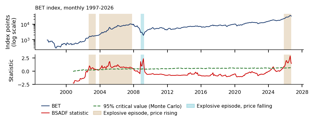
            For the monthly Nasdaq 100 (\(\hat\rho_1 = 0.05\); GSADF 3.08 with one lag against a critical value of 2.40) and weekly Bitcoin (\(\hat\rho_1 = 0.07\); GSADF 3.60 against 2.37), the conclusion is the same with one lag. Monthly BET returns are autocorrelated (\(\hat\rho_1 = 0.18\), Ljung–Box p = 0.008), and with one lag GSADF falls to 2.29, below its critical value of 2.39 (\(p = 0.063\)).

            The wild bootstrap does not fix this problem. It keeps the time pattern of the variance but not the autocorrelation, which independent signs destroy, and it does not cover infinite variance either.

            In brief

            Series\(\hat\rho_1\)Ljung–Box pGSADF, \(k = 0\)GSADF, \(k = 1\)95% critical
            value, \(k = 1\)
            Nasdaq 100, monthly\(0.05\)\(0.58\)\(2.57\)\(3.08\)\(2.40\)
            Bitcoin, weekly\(0.07\)\(0.35\)\(3.85\)\(3.60\)\(2.37\)
            BET, monthly\(0.18\)\(0.008\)\(2.90\)\(2.29\)\(2.39\)
            • The chapter's ADF regressions have no lags of \(\Delta y\); autocorrelated returns can distort their size
              • \(\hat\rho_1\): first-order autocorrelation of returns
              • Ljung–Box p: the test with 12 lags, not corrected for heteroskedasticity
              • \(k\): number of lags of \(\Delta y\) in the ADF regression
              • The Monte Carlo critical value is recomputed for the one-lag regression (2 000 paths)
            • Nasdaq 100 and Bitcoin: the conclusion is the same with one lag
            • BET: monthly returns are autocorrelated, and with one lag GSADF falls below its critical value (\(p = 0.063\))
            • The wild bootstrap keeps the time pattern of the variance, not the autocorrelation: independent signs destroy it
              • Nor does it cover infinite variance

            S&P Composite (Shiller) Price-Dividend Ratio, 1871–2026 (1/2)

            Slide 30 in the PDF
              Question for the room In May 2026, the S&P Composite price-dividend ratio is at its sample maximum, 91.2, but BSADF does not exceed its critical value. What does this comparison establish?
              Answer

              There is no explosiveness signal at this date under the chosen specification: the test looks for acceleration, not for a high level. In May 2026, BSADF is about 0.00, below the critical value 0.60. With the minimum duration L = 8, three episodes are retained: Aug 1917–Jun 1918 (an accelerating fall of the ratio), Nov 1928–Sep 1929 and May 1997–Aug 2001; another 46 exceedances form shorter runs. Local non-rejection does not establish the absence of a bubble. On the full sample, GSADF = 3.41 exceeds the 95% critical value, 2.39, while the full-sample ADF (−1.11) detects nothing.

              The chart is the chapter's central result. The top panel shows the S&P Composite price-dividend ratio, monthly from January 1871 to June 2026, on a log scale; the bottom panel shows the BSADF statistic with its 95% Monte Carlo critical value. The shaded areas are the date-stamped explosive episodes, beige when the ratio rises and blue when it falls.

              In brief

              S&P Composite (Shiller) Price-Dividend Ratio, 1871–2026 (2/2)

              Slide 31 in the PDF

              The series is the real price divided by the real dividend, with \(T = 1{,}865\) monthly changes and a minimum window of 96 months. GSADF is 3.41, above the 95% critical value of 2.39 and the 99% value of 2.88, while the full-sample ADF statistic, −1.11, sees nothing. Three episodes are date-stamped: Aug 1917–Jun 1918, Nov 1928–Sep 1929 and May 1997–Aug 2001.

              The direction of each episode matters. The 1917–1918 episode is an accelerating fall of the ratio, explosive but not a bubble, so the direction must always be reported; in the chart legend "price rising/falling" refers to the plotted series, here the ratio. A ratio can also explode through its denominator, so both price and dividend must be checked.

              The level of the ratio is not the same as explosiveness. The dot-com peak was 90.2 in August 2000, against a long-run mean of 29.8, but the sample maximum, 91.2 in May 2026, lies in no episode. The result supports a description: the test dates explosive episodes but does not separate them from explosive fundamentals.

              In brief

              • Real price over real dividend, monthly, Jan 1871–Jun 2026
                • \(T = 1\,865\), minimum window 96 months
                • In the chart legend, “price rising/falling” refers to the plotted series, here the ratio
              • GSADF \(= 3.41\) vs 95% critical value \(2.39\) (99%: \(2.88\))
                • The full-sample ADF (\(-1.11\)) sees nothing
              • Episodes: Aug 1917–Jun 1918; Nov 1928–Sep 1929; May 1997–Aug 2001
                • 1917–1918: an accelerating fall of the ratio, explosive but not a bubble: always report the direction
              • Dot-com: peak \(90.2\) in Aug 2000, long-run mean \(29.8\)
                • The sample maximum, \(91.2\) in May 2026, lies in no episode: a high ratio is not necessarily explosive
              • A ratio can explode through its denominator: check both price and dividend
              • Type of evidence: description (it shows what happened in the data, without testing a cause)
                • the test dates explosive episodes; it does not separate them from explosive fundamentals
              MFM_ch17_sp_pd

              The Dow Jones, 1921–1932: The Tests in Real Time (1/2)

              Slide 32 in the PDF

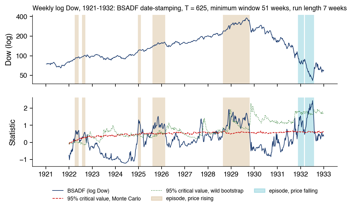
              The chart applies BSADF date-stamping to the log weekly closes of the Dow Jones, 1921–1932. At the top, the index on a log scale; at the bottom, the BSADF statistic with the 95% critical values by Monte Carlo and by wild bootstrap. The shaded areas are the episodes dated with the Monte Carlo values: beige when the price rises, blue when it falls.

              In brief

              The Dow Jones, 1921–1932: The Tests in Real Time (2/2)

              Slide 33 in the PDF

              The series has \(T = 625\) weekly changes, with a minimum window of 51 weeks and a minimum episode length of 7 weeks. GSADF is 2.44, above the 95% Monte Carlo critical value of 2.30 but below the wild bootstrap one, 3.92. The very high volatility of 1929–1932 therefore changes the conclusion: with heteroskedasticity-robust critical values, the overall test does not reject the null.

              The main episode starts, dated in hindsight, on 25 August 1928 and ends on 19 October 1929. In real time the alarm comes 7 weeks later, on 6 October 1928, with the index at 240.17, and the index then rises another 59% to the peak: the alarm comes early and does not date the end. The signal ends in the week before Black Thursday, because the test measures the acceleration of the price, and the rise had stopped in September.

              Four other, shorter rising episodes appear in 1922–1926, and over the following two years the index fell by at most 19% after them. The episodes of 1931–1932 are accelerating declines, hence not bubbles. Shiller's price-dividend ratio dates a close episode, November 1928–September 1929.

              In brief

              • Log weekly closes, 1921–1932: \(T = 625\), minimum window 51 weeks, minimum run length 7 weeks
              • GSADF \(= 2.44\): above the 95% Monte Carlo critical value (\(2.30\)), below the wild bootstrap one (\(3.92\))
                • The volatility of 1929–1932 changes the conclusion: with heteroskedasticity-robust critical values the overall test does not reject the null
              • Main episode: 25 Aug 1928–19 Oct 1929
                • The start is dated in hindsight: the real-time alarm comes 7 weeks later, on 6 Oct 1928, with the index at 240.17
                • The index then rises another 59% to the peak: the alarm comes early and does not date the end
                • The signal ends in the week before Black Thursday: the test measures acceleration, and the rise had stopped in September
              • Four other, shorter rising episodes, 1922–1926: falls of at most 19% over the following two years
              • 1931–1932: episodes of accelerating decline, hence not bubbles
              • The Shiller price-dividend ratio dates a close episode: Nov 1928–Sep 1929

              Bitcoin: Explosive Episodes (1/2)

              Slide 34 in the PDF
                Question for the room Bitcoin: we keep the Monte Carlo critical values and reduce only the minimum duration from L = 7 to L = 3 weeks. Which March–April 2024 episode is retained?
                Answer

                1–15 March 2024. With the Monte Carlo critical values, BSADF exceeds the threshold on 1–15 March (three consecutive weeks) and on 29 March–5 April (two). Reducing L changes the duration filter, not the statistics or the thresholds: the three-exceedance run becomes an episode, the two-exceedance run stays excluded, and the gap between them prevents their merger. With L = 7, the episodes are Apr 2017–Jun 2018 and Dec 2020–May 2021; with the wild bootstrap, May 2017–Jan 2018 and Dec 2020–Feb 2021. GSADF = 3.85 rejects the null with both critical values (2.27 and 2.82).

                The chart applies the same procedure to weekly Bitcoin prices: the log close and the BSADF statistic with its 95% critical values, by Monte Carlo and by wild bootstrap.

                Bitcoin: Explosive Episodes (2/2)

                Slide 35 in the PDF

                The data are weekly log closes in US dollars (USD), 2014–2026, with \(T = 626\) and a minimum window of 51 weeks. GSADF is 3.85, so the null is rejected with either 95% critical value: 2.27 by Monte Carlo and 2.82 by wild bootstrap.

                The two sets of critical values date slightly different episodes. With Monte Carlo values the episodes are Apr 2017–Jun 2018 and Dec 2020–May 2021; with wild-bootstrap values they shrink to May 2017–Jan 2018 and Dec 2020–Feb 2021. The 2017 episode starts 8 months before the peak of 16 December 2017 and ends 6 months after it.

                The rise to new highs in 2024–2025 is not flagged: steady growth is not explosive acceleration. As for the S&P, the result supports a description of the price path.

                In brief

                • Weekly log closes in US dollars (USD) 2014–2026, \(T = 626\), minimum window 51 weeks
                • GSADF \(= 3.85\): rejected with either critical value
                  • 95% critical value: Monte Carlo \(2.27\), wild bootstrap \(2.82\)
                • Episodes with Monte Carlo critical values: Apr 2017–Jun 2018; Dec 2020–May 2021
                  • With wild bootstrap critical values: May 2017–Jan 2018; Dec 2020–Feb 2021
                • The 2017 episode starts 8 months before the peak of 16 Dec 2017 and ends 6 months after it
                • The 2024–2025 rise to new highs is not flagged: steady growth is not explosive acceleration
                • Type of evidence: description
                MFM_ch17_bitcoin

                Date-Stamping Is a Multiple Test: Bitcoin (1/2)

                Slide 36 in the PDF

                Comparing BSADF with its critical value at each of 626 weeks makes hundreds of dependent tests. The relevant error rate is the family-wise error rate (FWER), the probability of at least one false alarm over the whole monitoring window. In 2,000 random walks with the Bitcoin \(T\) and minimum window \(w_0\), BSADF crosses its pointwise critical value at least once in 95% of paths and produces an "episode" in 59%.

                Phillips & Shi (2020) propose to bootstrap the maximum of BSADF over the last \(\tau_b\) monitoring dates, here \(\tau_b = 104\) weeks. The resulting threshold is 1.75, against Monte Carlo pointwise values of at most 0.71. Applied to the whole history, the threshold leaves one episode, Oct 2017–Jan 2018; the 2020–2021 episode found with pointwise values does not survive.

                This is a sensitivity check, not proved FWER control (design in the Appendix). The threshold is calibrated on 104 weeks; applied to all 626, it is crossed under the null in 19% of paths, while a confirmed episode, 7 consecutive crossings, occurs in 2% of paths.

                In brief

                • BSADF vs its critical value at each of 626 weeks: hundreds of dependent tests
                • Family-wise error rate (FWER)
                  • The probability of at least one false alarm over the whole monitoring window
                  • 2 000 random walks with the Bitcoin \(T\) and \(w_0\): a crossing in \(95\%\), an “episode” in \(59\%\) of paths
                • Phillips and Shi: bootstrap the maximum of BSADF Phillips & Shi (2020)
                  • Over the last \(\tau_b\) monitoring dates; here \(\tau_b = 104\) weeks
                  • Phillips–Shi threshold: \(1.75\), against Monte Carlo pointwise values of at most \(0.71\)
                • Episodes above the Phillips–Shi threshold applied to the whole history: Oct 2017–Jan 2018
                  • The 2020–2021 episode found with Monte Carlo pointwise values does not survive
                • A sensitivity check, not proved FWER control (design in the Appendix)
                  • The threshold is calibrated on 104 weeks; applied to all 626, under the null it is crossed in \(19\%\) of paths
                  • A confirmed episode (7 consecutive crossings) occurs in \(2\%\) of paths
                MFM_ch17_inference

                Date-Stamping Is a Multiple Test: Bitcoin (2/2)

                Slide 37 in the PDF
                  Question for the room Over a history of 626 weekly changes, we compare the 576 defined BSADF values with their pointwise 95% critical values. Under the null (random walk), in what proportion of paths does at least one exceedance occur?
                  Answer

                  About 95%: on 2,000 random-walk paths, an exceedance occurs in 95% of them, and an "episode" of at least seven consecutive exceedances in 59%. The 5% option is the nominal level of a single comparison. The 19% option comes from applying the Phillips–Shi threshold, calibrated on 104 weeks, to the whole history: a sensitivity analysis, not family-wise error control. The threshold is 1.75, against pointwise Monte Carlo values of at most 0.71; with it a single episode remains, Oct 2017–Jan 2018.

                  The chart compares, week by week, the Bitcoin BSADF statistic with the pointwise Monte Carlo critical values and with the Phillips–Shi threshold of 1.75.

                  Real Time vs Hindsight

                  Slide 38 in the PDF

                  The table compares the hindsight dating of five episodes with what a real-time monitor would have seen. The start is the first exceedance of the chain of BSADF runs that leads to the peak, known only in hindsight; the confirmation date comes after \(L\) consecutive exceedances and is available in real time. The rise is measured from confirmation to the peak, and the fall to the lowest close within two years (one year for GameStop).

                  Even at confirmation the tests warn early: the lead from confirmation to the peak is 51 months for the Nasdaq 100, 39 months for BET, 6 months for Bitcoin in 2017, 2 months for Bitcoin in 2021 and 0.2 months for GameStop. They do not time the crash (Phillips, Shi & Yu, 2015b). Selling at confirmation would have missed most of the rise: +716% for the Nasdaq 100, +299% for BET and +590% for Bitcoin in 2017.

                  The five episodes are episodes that ended in crashes, so the lead is not a hit rate of the alarms. The table supports a description of how early the test confirms such episodes.

                  In brief

                  EpisodeStart / PeakConfirmedLead
                  (months)
                  Lead from
                  conf.
                  Rise after
                  conf.
                  Fall after
                  peak
                  Nasdaq 100, monthlyJun 1995 / Mar 2000Dec 1995\(57\)\(51\)\(+716\%\)\(-76\%\)
                  BET, monthlyNov 2003 / Jul 2007Apr 2004\(44\)\(39\)\(+299\%\)\(-83\%\)
                  Bitcoin 2017, weeklyApr 2017 / Dec 2017Jun 2017\(8\)\(6\)\(+590\%\)\(-83\%\)
                  Bitcoin 2021, weeklyDec 2020 / Apr 2021Feb 2021\(4\)\(2\)\(+66\%\)\(-75\%\)
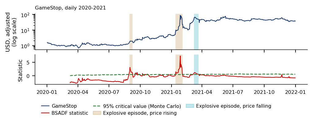
                  GameStop, daily13 Jan 2021 / 27 Jan 202122 Jan 2021\(0.5\)\(0.2\)\(+435\%\)\(-88\%\)
                  • Columns (caveats in the Appendix)
                    • Start: first exceedance of the chain of BSADF runs that leads to the peak (hindsight); confirmed: after \(L\) consecutive exceedances (real time)
                    • Lead: months to the peak, from the start or from confirmation; rise: from confirmation to the peak; fall: to the lowest close within 2 years (GameStop: within 1 year)
                  • Even at confirmation the tests warn early, but they do not time the crash Phillips, Shi & Yu (2015b)
                    • Selling at confirmation would have missed most of the rise
                  • Type of evidence: description
                    • five episodes that ended in crashes: the lead is not a hit rate of the alarms

                  Reading the Real-Time Table

                  Slide 39 in the PDF

                  The chain rule allows gaps inside an episode: at most 93 days for monthly data, 28 days for weekly data and 10 days for the daily GameStop series. For the Nasdaq 100 the chain joins 3 runs and starts in June 1995. A strict rule that keeps only the run containing the peak would start in September 1998 and confirm in March 1999, with leads of 18 and 12 months instead of 57 and 51. For BET, Bitcoin and GameStop the two rules give the same start.

                  Two tables give two falls for the same dot-com crash. This table reports −76%, the lowest daily close within two years of the peak; the table of nine episodes reports −83% within four years, because the trough of October 2002 came 30 months after the peak, outside the two-year window.

                  For Bitcoin in 2021 the peak in this table is the local high of 13 April 2021, not the all-time high of 8 November 2021. The explosive chain ended in May 2021, and the later high came after a deep fall and a slower recovery that BSADF did not flag.

                  In brief

                  • Largest gap inside a chain
                    • 93 days for monthly data
                    • 28 days for weekly data
                    • 10 days for daily GameStop
                  • Nasdaq 100: the chain joins 3 runs, from Jun 1995
                    • The strict rule keeps only the run containing the peak
                    • Strict rule: start Sep 1998, confirmed Mar 1999, leads \(18\) and \(12\) months instead of \(57\) and \(51\)
                    • For BET, Bitcoin and GameStop the two rules give the same start
                  • Two falls for the same dot-com crash
                    • This table: \(-76\%\), the lowest daily close within 2 years of the peak
                    • Nine Episodes table: \(-83\%\) within 4 years; the trough of Oct 2002 came \(30\) months after the peak, outside the 2-year window
                  • Bitcoin 2021: the peak here is the local high of 13 Apr 2021, not the all-time high of 8 Nov 2021
                    • The explosive chain ended in May 2021; the later high came after a deep fall and a slower recovery that BSADF did not flag

                  Section summary

                  Explosiveness is tested in the right tail, on windows, and dated with BSADF and a minimum duration. On the S&P price-dividend ratio and on Bitcoin the tests flag the known episodes, but the critical values depend on volatility, lags and the number of dates monitored, and in real time the confirmation comes well before the peak without timing the crash.

                  The Log-Periodic Power Law (LPPLS)

                  The explosiveness tests say that an episode is under way but not when it ends. The LPPLS model goes further: it gives the run-up a specific shape, faster-than-exponential growth with accelerating oscillations, and a parameter for the critical time at which the bubble is most likely to end. The section defines the model, the conditions for a qualified fit and the confidence indicator that pools many windows, and then tests whether the indicator's signals are followed by falls more often than chance.

                  Crashes as Critical Points

                  Slide 40 in the PDF

                  The question is whether the shape of the run-up can tell when the bubble ends. In the model of Johansen, Ledoit and Sornette (JLS) (Johansen, Ledoit & Sornette, 2000), imitation among traders makes the hazard rate of a crash, the crash probability per unit time given no crash yet, rise as a critical time \(t_c\) approaches.

                  Rational investors stay in the market only if the price grows fast enough to pay for the rising crash risk. The result is faster-than-exponential growth, decorated by oscillations that speed up near \(t_c\). The critical time is the most probable end of the bubble, not a certain crash date (Sornette, 2017).

                  In brief

                  Crashes as Critical Points Didier Sornette, ETH (Eidgenössische Technische Hochschule) Zurich Photo: Didier Sornette (2012); CC BY-SA 3.0 (Germany); Wikimedia Commons
                  • Question: can the shape of the run-up tell when the bubble ends?
                  • Johansen, Ledoit and Sornette (JLS) Johansen, Ledoit & Sornette (2000)
                    • Imitation among traders makes the hazard rate of a crash rise as a critical time \(t_c\) approaches
                    • Hazard rate: the crash probability per unit time, given no crash yet
                  • Rational investors stay in only if the price grows fast enough
                    • The extra growth pays for the rising crash risk
                  • Result: faster-than-exponential growth
                    • Decorated by oscillations that speed up near \(t_c\)
                  • \(t_c\) is the most probable end of the bubble, not a certain crash date Sornette (2017)

                  The LPPLS Equation

                  Slide 41 in the PDF

                  The log price follows

                  \[\ln p(t) = A + B\,(t_c - t)^m + C\,(t_c - t)^m \cos\!\big(\omega \ln(t_c - t) - \phi\big), \qquad t < t_c,\]
                  (17.10)

                  a power-law trend towards the critical time plus oscillations whose frequency rises as \(t_c\) approaches; \(p(t)\) is the price at time \(t\).

                  \(A\) is the log price at \(t_c\). \(B < 0\) gives the super-exponential trend of a rising bubble, and \(0 < m < 1\) is the power-law exponent. The growth rate of the trend, \(-Bm(t_c - t)^{m-1}\), rises without bound as \(t \to t_c\), which is the finite-time singularity. \(C\), \(\omega\) and \(\phi\) are the amplitude, the angular log-frequency and the phase of the log-periodic oscillations.

                  The model has seven parameters: \(A\), \(B\), \(C\) and \(\phi\), which enter linearly after a reparametrisation, and the nonlinear \(t_c\), \(m\) and \(\omega\). LPPL denotes the log-periodic power law pattern itself, and LPPLS the model with the finite-time singularity at \(t_c\).

                  In brief

                  • \(\ln p(t) = A + B\,(t_c - t)^m + C\,(t_c - t)^m \cos\!\left(\omega \ln(t_c - t) - \phi\right)\), \(\ t < t_c\)
                    • In words: the log price is a power-law trend towards the critical time plus oscillations whose frequency rises as \(t_c\) approaches; \(p(t)\): price at time \(t\); \(t_c\): critical time
                  • \(A\): log price at \(t_c\)
                  • \(B < 0\): the super-exponential trend for a rising bubble
                  • \(0 < m < 1\): power-law exponent
                    • The growth rate of the power-law trend, \(-B m (t_c - t)^{m - 1}\), rises without bound as \(t \to t_c\)
                  • \(C\), \(\omega\), \(\phi\): amplitude, angular log-frequency and phase of the log-periodic oscillations
                  • Seven parameters: \(A, B, C, \phi, t_c, m, \omega\); after the rewrite with \(C_1 = C\cos\phi\), \(C_2 = C\sin\phi\) only \(t_c, m, \omega\) stay nonlinear (Further Topics)
                  • LPPL: the log-periodic power law pattern
                    • LPPLS: the model with the finite-time singularity at \(t_c\)

                  Qualified Fits: Conditions on the Parameters and the Residuals

                  Slide 42 in the PDF

                  A fit of (17.10) on an estimation window \([t_1, t_2]\) is qualified if it passes all the conditions of Shu & Zhu (2020a) (eq. 12) and has \(B < 0\) for a rising bubble. The parameter bounds are \(m \in [0.01, 0.99]\), \(\omega \in [2, 25]\) and \(t_c \in [t_2,\, t_2 + (t_2 - t_1)/5]\), and the damping condition \(m|B|/(\omega|C|) \ge 1\) is already imposed in the search.

                  Two conditions guard against spurious oscillations and poor fits:

                  1. The number of oscillations, counted in half-periods, \(O = \frac{\omega}{\pi}\ln\frac{t_c - t_1}{t_c - t_2}\), must be at least 2.5, so that the oscillations are not noise.
                  2. The largest relative error of the fitted price, \(\max_t |\hat p_t - p_t|/p_t\), must not exceed 0.15.

                  Two further filters check the residuals. The Lomb periodogram, which measures spectral power for unevenly spaced points (here the values of \(\ln(t_c - t)\)), is applied to the detrended residual \((t_c - t)^{-m}(\ln p_t - A - B(t_c - t)^m)\) at the nominal level 0.10. The residual \(\ln\hat p_t - \ln p_t\) must also be stationary: the Dickey–Fuller and Phillips–Perron tests, the latter a Dickey–Fuller-type test with a nonparametric correction for serial correlation, must reject a unit root at the nominal level 0.10. Both are heuristic filters, since the trend is fitted on the same data and the p-values are not calibrated.

                  In brief

                  • A fit on the estimation window \([t_1, t_2]\) is qualified
                    • If it passes all conditions of Shu & Zhu (2020a, eq. 12)
                    • And \(B < 0\) for a rising bubble
                    • \(m \in [0.01, 0.99]\), \(\omega \in [2, 25]\), \(t_c \in [t_2, t_2 + (t_2 - t_1)/5]\)
                    • Damping \(\frac{m|B|}{\omega|C|} \ge 1\) (already imposed in the search)
                    • Number of oscillations (half-periods) \(O = \frac{\omega}{\pi}\ln\frac{t_c - t_1}{t_c - t_2} \ge 2.5\), so the oscillations are not noise
                    • Largest relative error of the fitted price \(\max_t |\hat p_t - p_t|/p_t \le 0.15\)
                  • Lomb periodogram of the detrended residual \((t_c - t)^{-m}(\ln p_t - A - B(t_c - t)^m)\)
                    • A heuristic filter with nominal level \(0.10\): the trend is fitted on the same data, so the p-value is not calibrated
                    • Lomb periodogram: spectral power for unevenly spaced points, here the values of \(\ln(t_c - t)\)
                  • The residual \(\ln \hat p_t - \ln p_t\) must be stationary
                    • Dickey–Fuller and Phillips–Perron reject a unit root at the nominal level \(0.10\), again a heuristic filter
                    • Phillips–Perron: a Dickey–Fuller-type test with a nonparametric correction for serial correlation

                  LPPLS on Bitcoin, 2017 (1/2)

                  Slide 43 in the PDF
                    Question for the room The LPPLS fit on Bitcoin up to 15 November 2017 has a maximum relative error of 0.42, and the qualification limit is 0.15. By at least what percentage must the error fall to pass this filter?
                    Answer

                    64.3% = (0.42 − 0.15)/0.42. The difference of 0.27 is 27 percentage points, not a relative reduction of 27%. The value 35.7% = 0.15/0.42 is the part of the initial error that may remain. The fit puts tc on 21 Dec 2017, 5 days after the peak, and m = 0.95, ω = 10.54 and B = −2.62 lie in the required ranges; passing the error filter does not guarantee passing the other conditions. No fit on this grid is qualified.

                    The chart shows the LPPLS fit on daily Bitcoin log prices from 1 January to 15 November 2017, the estimated critical time and the price path after the end of the window, which is out of sample.

                    In brief

                    LPPLS on Bitcoin, 2017 (2/2)

                    Slide 44 in the PDF

                    The fit reproduces the 2017 trend and oscillations, with \(m = 0.95\), \(\omega = 10.54\) and \(B = -2.62\). The estimated critical time is 21 December 2017; the actual peak was 16 December 2017.

                    The fit nevertheless does not pass the filter. Its largest relative error exceeds 0.15, and the damping \(D = 1.00\) sits at the bound imposed in the search, while the exact condition \(m|B| \ge |C|\sqrt{m^2+\omega^2}\) fails, with a ratio of 0.996. A fit can look convincing and still fail the qualification conditions.

                    In brief

                    • Fit on daily log prices, 1 January to 15 November 2017
                      • The path after 15 November is out of sample
                    • The fit reproduces the 2017 trend and oscillations, but its largest relative error exceeds \(0.15\)
                      • \(m = 0.95\), \(\omega = 10.54\), \(B = -2.62\)
                      • Damping ratio \(\frac{m|B|}{\omega|C|} = 1.00\), at the bound imposed in the search; the exact condition \(m|B| \ge |C|\sqrt{m^2 + \omega^2}\) fails (ratio \(0.996\))
                    • Estimated \(t_c\): 21 Dec 2017; actual peak: 16 Dec 2017
                    • The fit does not pass the filter, even though it looks convincing
                    MFM_ch17_lppls

                    How Stable Is the Critical Time? (1/2)

                    Slide 45 in the PDF
                      Question for the room Four of the 20 LPPLS fits on Bitcoin before the peak put tc within 30 days of the peak. What does the 20% proportion represent?
                      Answer

                      The share of the fits on this grid that meet the retrospective criterion. The denominator is 20 fits, not 20 independent crashes; the proportion is neither a calibrated crash probability nor the confidence level of an interval. The 20 fits put tc between Oct 2017 and Feb 2018, with a mean absolute error of 48 days; for the Nasdaq 100 the mean error is 71 days. None of these fits is qualified.

                      Each point of the chart is one LPPLS fit on a window with a fixed start, ending on the date on the horizontal axis, refitted every 7 days; the vertical axis gives the estimated critical time.

                      In brief

                      How Stable Is the Critical Time? (2/2)

                      Slide 46 in the PDF

                      A good in-sample fit is not a forecast. For Bitcoin, the 20 fits before the peak placed \(t_c\) between October 2017 and February 2018, with a mean absolute error of 48 days, and only 20% of the fits fell within 30 days of the peak. For the Nasdaq 100, the 30 fits before the peak placed \(t_c\) between December 1999 and September 2000, with a mean absolute error of 71 days.

                      The constraint \(t_c \ge t_2\) is part of the search, so the estimated critical time always lies after the end of the window and moves with it; this is a constraint, not a forecast. None of the fits before the peak is qualified, 0% for Bitcoin and 0% for the Nasdaq 100. One window is not enough, which motivates the confidence indicator.

                      In brief

                      • A good in-sample fit is not a forecast
                        • Each point: one fit on a window with a fixed start, ending on the date on the horizontal axis (every 7 days)
                      • Bitcoin: before the peak (20 fits) \(t_c\) ranged from Oct 2017 to Feb 2018
                        • Mean absolute error \(48\) days; within 30 days of the peak: \(20\%\) of the fits
                      • Nasdaq 100: before the peak (30 fits) \(t_c\) ranged from Dec 1999 to Sep 2000
                        • Mean absolute error \(71\) days; \(t_c \ge t_2\) is a constraint of the search, not a forecast
                      • Qualified fits before the peak: \(0\%\) (Bitcoin), \(0\%\) (Nasdaq 100)
                        • One window is not enough: the confidence indicator pools many windows
                      MFM_ch17_lppls

                      The LPPLS Confidence Indicator: Definition and Evaluation

                      Slide 47 in the PDF

                      At each date \(t_2\) the confidence indicator fits many windows \([t_2 - \ell, t_2]\) and reports the share of qualified fits (Demirer et al., 2019):

                      \[I_{t_2} = \frac{1}{N}\sum_{\ell} \mathbf{1}\{\text{the fit on } [t_2 - \ell,\, t_2] \text{ is qualified}\},\]
                      (17.11)

                      a number between 0 and 1. The grid of Shu & Zhu (2020a) has \(N = 141\) windows, with \(\ell\) from 750 down to 50 observations in steps of 5; \(t_2\) moves every 5 observations (calendar days for Bitcoin) and only data up to \(t_2\) are used. A high share means that the bubble signature is robust to the choice of window. The birth of a bubble is easier to diagnose than its burst (Demos & Sornette, 2017).

                      The evaluation asks whether a signal, \(I_{t_2} > 0\), is followed by a fall of at least 20% within 90 days more often than a date without a signal. The fall is measured from the price on the signal date, and only dates whose next 90 calendar days are fully observed are used. The 20% threshold and the 90-day horizon are fixed in advance; the AI section checks a grid of 4 horizons and 3 thresholds.

                      In brief

                      • At each date \(t_2\), fit many windows \([t_2 - \ell, t_2]\) and report the share of qualified fits Demirer et al. (2019)
                        • \(I_{t_2} = \frac{1}{N}\sum_{\ell} \mathbf{1}\{\text{the fit on } [t_2 - \ell, t_2] \text{ is qualified}\}\), between 0 and 1
                        • Grid of Shu and Zhu: \(N = 141\) windows, \(\ell\) from 750 down to 50 observations in steps of 5 Shu & Zhu (2020a)
                        • \(t_2\) moves every 5 observations (calendar days for Bitcoin); data up to \(t_2\) only
                      • A high share means the bubble signature is robust to the choice of window
                      • The birth of a bubble is easier to diagnose than its burst Demos & Sornette (2017)
                      • Evaluation: is a signal (\(I_{t_2} > 0\)) followed by a fall of at least \(20\%\) within 90 days
                        • More often than no signal?
                        • Fall measured from the price on the signal date
                        • Only dates whose next 90 calendar days are fully observed
                        • The \(20\%\) threshold and the 90-day horizon are fixed in advance; the AI section checks a grid of 4 horizons \(\times\) 3 thresholds

                      Bitcoin: LPPLS Confidence Indicator

                      Slide 48 in the PDF
                        Question for the room After an LPPLS signal (positive indicator), is a 20% fall within 90 days more frequent than without one?
                        Answer

                        No. The fall follows 22% of the 82 signals and 37% of the dates without a signal (709 dates evaluated). The difference, −15.5 percentage points, has a block-bootstrap CI of [−30.0, 1.8]: the evidence is weak, and the sign is the opposite of the expected one.

                        The chart shows the Bitcoin price with the confidence indicator (17.11) as bars on the right axis, every 5 days from 2016 to 2026. The reading is on the results slide below.

                        LPPLS: Qualification Filters

                        Slide 49 in the PDF
                          Question for the room For Bitcoin, 10.2% of the windows pass the relative-error filter on its own, while 0.4% pass all the conditions up to and including the Lomb test. What percentage of all windows does the Lomb test reject on its own?
                          Answer

                          It cannot be determined from these two shares. 0.4% is the intersection of all the preceding conditions with the Lomb test; its complement, 99.6%, is not the rejection rate of the Lomb test alone. Computing 1 − 0.4/10.2 = 96.1% wrongly attributes to the Lomb test every elimination between the error filter and the cumulative result. Taken separately, a relative error of at most 0.15 is passed by 10% of the windows, against about a third for the conditions on m, ω, tc and the number of oscillations. After all conditions, 0.3% of the Bitcoin windows and 3.5% of the Nasdaq 100 windows remain qualified, hence the small values of the indicator (at most 0.18).

                          The chart shows, for Bitcoin and for the Nasdaq 100, the share of all windows that pass each qualification condition. The rows are cumulative: each condition counts only the windows that pass every condition above it.

                          The Confidence Indicator and Its Filters: Results

                          Slide 50 in the PDF

                          The price panel plots the Bitcoin price and the share of the 141 windows with a qualified fit; the filter panel shows which conditions remove most windows, with the Lomb and residual tests counting only windows that pass every condition above them. The indicator is positive on 14% of the 2017 dates, 3% in 2021 and 12% in the other years, with a maximum of 0.18 in December 2020.

                          A fall of 20% within 90 days followed 22% of signals and 37% of no-signal dates, over 709 Bitcoin dates. For the Nasdaq 100, 1997–2026, the shares are 4% and 11%, over 1,483 dates. The raw difference is not yet evidence: signals come in runs and the 90-day outcome windows overlap, so the test on the next slide accounts for the dependence.

                          In brief

                          • Price panel: Bitcoin price and the share of the 141 windows with a qualified fit
                            • The share is shown as bars on the right axis, every 5 days, 2016–2026
                            • Filter panel: share of all windows passing each condition, Bitcoin and, for comparison, the Nasdaq 100
                            • Cumulative rows: the Lomb and residual tests count only windows that pass every condition above them
                          • Positive on \(14\%\) of the 2017 dates, \(3\%\) in 2021, \(12\%\) in other years
                            • Maximum \(0.18\) in Dec 2020
                          • A \(20\%\) fall within 90 days followed \(22\%\) of signals, \(37\%\) of no-signal dates
                            • Bitcoin: 709 dates; Nasdaq 100, 1997–2026: \(4\%\) vs \(11\%\) (1483 dates)
                          • The raw difference is not yet evidence (test on the next slide)
                            • Signals come in runs and the 90-day outcome windows overlap
                          MFM_ch17_lppls_confidence

                          Is the Indicator Better than Chance? A Test (1/2)

                          Slide 51 in the PDF

                          The null hypothesis is that a fall of at least 20% within 90 days is equally likely after a signal and after no signal:

                          \[H_0:\ P(\text{fall} \ge 20\% \text{ within 90 days} \mid \text{signal}) = P(\cdot \mid \text{no signal}).\]

                          The statistic is \(\Delta = \hat p_{\text{on}} - \hat p_{\text{off}}\), the share of signal dates followed by such a fall minus the share of no-signal dates.

                          Dates 5 days apart share up to 85 of their 90 outcome days, so the outcomes are strongly dependent. The two-sample \(z\)-test assumes independent dates and therefore understates the standard error. Two dependence-robust alternatives are used: a circular block bootstrap of the (signal, outcome) pairs with blocks of 90 days and 9,999 replications, and a linear probability regression of the outcome on the signal with Newey–West standard errors with 18 lags, which cover 90 days at a 5-day spacing.

                          In brief

                          • \(H_0\colon P(\text{fall} \ge 20\% \text{ within 90 days} \mid \text{signal}) = P(\cdot \mid \text{no signal})\)
                            • Statistic \(\Delta = \hat p_{\text{on}} - \hat p_{\text{off}}\): share of signal dates followed by such a fall minus the share of no-signal dates
                          • Overlap: dates 5 days apart share up to 85 of their 90 outcome days
                            • The two-sample \(z\)-test assumes independent dates and so understates the standard error
                          • Dependence-robust inference
                            • Circular block bootstrap of the (signal, outcome) pairs: blocks of 90 days, 9 999 replications
                            • Linear probability regression of the outcome on the signal, with Newey–West standard errors with 18 lags (90 days at 5-day spacing)

                          Is the Indicator Better than Chance? A Test (2/2)

                          Slide 52 in the PDF

                          For Bitcoin, \(\Delta = -15.5\) percentage points, with a 95% block-bootstrap CI of [−30.0, 1.8], which contains zero. The block standard error is 8.1, against 5.0 under independence. With blocks of 36 and 72 dates the intervals are [−30.8, 2.4] and [−30.2, 1.0]. The Newey–West regression gives a two-sided \(p = 0.049\) for \(H_0: \Delta = 0\), at the edge of the 5% level; the percentile interval and the Newey–West \(t\)-test use different standard errors and need not agree near the boundary.

                          The evidence is weak, and the point estimate is negative: if anything, falls are less frequent after signals, because signals also occur in steady rises, not just before crashes. The negative direction was not stated in advance, so the one-sided \(p = 0.024\) is only exploratory. The result supports, at most, a weak association between the signal and later falls, with a negative point estimate.

                          In brief

                          • Bitcoin: \(\Delta = -15.5\) percentage points, 95% block-bootstrap CI \([-30.0, 1.8]\), which contains zero
                            • Block SE \(8.1\) vs independent-data SE \(5.0\)
                            • Blocks of 36 and 72 dates: CI \([-30.8, 2.4]\) and \([-30.2, 1.0]\)
                          • Newey–West regression: two-sided \(p = 0.049\) for \(H_0\colon \Delta = 0\), at the edge of the 5% level
                            • The percentile CI and the Newey–West \(t\)-test use different standard errors, so they need not agree near the 5% boundary
                          • Weak evidence, and the point estimate is negative: if anything, a lower crash rate after signals
                            • Signals come in steady rises, not just before crashes
                            • The negative direction was not stated in advance: the one-sided \(p = 0.024\) is only exploratory
                          • Type of evidence: association
                            • between the signal and later falls: weak, and the point estimate is negative

                          Section summary

                          The LPPLS model gives a run-up a shape and a critical time, but single fits are unstable and rarely pass the qualification conditions. Pooled over 141 windows, the confidence indicator signals on a minority of dates, and its signals are not followed by more Bitcoin falls of 20% than no-signal dates.

                          Regime-Switching Models

                          Explosiveness tests and LPPLS look for the shape of a bubble. A regime-switching model takes a different view: it describes run-ups and crashes as alternating risk states, without dating a bubble or modelling fundamental value. The section estimates a two-regime model on weekly Nasdaq 100 returns and tests the number of regimes with a bootstrap likelihood ratio.

                          The Markov-Switching Model

                          Slide 53 in the PDF

                          The question is whether run-ups and crashes can be described as alternating risk states. In the model of Hamilton (1989), the weekly log return in percent, \(r_t = 100\ln(P_t/P_{t-1})\), follows

                          \[r_t = \mu_{s_t} + \sigma_{s_t}\varepsilon_t, \qquad \varepsilon_t \sim N(0,1), \qquad s_t \in \{1, 2\},\]
                          (17.12)

                          where the regime \(s_t\) is unobserved. Each regime has its own mean \(\mu\) and volatility \(\sigma\), so that one can be read as a calm regime and the other as a turbulent one.

                          The regimes follow a Markov chain with transition probabilities \(p_{ij} = P(s_t = j \mid s_{t-1} = i)\), and the expected duration of regime \(i\) is \(1/(1 - p_{ii})\). The parameters are estimated by maximum likelihood with the Hamilton filter, which updates \(P(s_t = j \mid r_1, \dots, r_t)\) week by week.

                          Two probabilities of the regime are reported:

                          • the filtered probability uses the returns up to \(t\) for given parameters;
                          • the smoothed probability uses the whole sample and is a hindsight measure.

                          Because the parameters here are estimated on the full sample, the filtered probabilities are only pseudo real time; genuine real time requires parameters re-estimated with data up to each \(t\).

                          In brief

                          • Question: can run-ups and crashes be described as alternating risk states, without dating a bubble?
                          • Weekly log return \(r_t = \mu_{s_t} + \sigma_{s_t}\varepsilon_t\), \(\varepsilon_t \sim N(0, 1)\), regime \(s_t \in \{1, 2\}\) unobserved Hamilton (1989)
                            • \(r_t = 100\ln(P_t/P_{t-1})\), in %
                            • Each regime has its own mean \(\mu\) and volatility \(\sigma\): a calm and a turbulent regime
                          • Regimes follow a Markov chain: \(p_{ij} = P(s_t = j \mid s_{t-1} = i)\)
                            • Expected duration of regime \(i\): \(1/(1 - p_{ii})\)
                          • Estimation by maximum likelihood with the Hamilton filter
                            • The filter updates \(P(s_t = j \mid r_1, \dots, r_t)\) week by week
                          • Filtered probability: returns up to \(t\) for given parameters
                          • Smoothed probability: the whole sample (hindsight)
                            • Our parameters are estimated on the full sample, so our filtered probabilities are only pseudo real time; genuine real time needs parameters re-estimated with data up to \(t\)

                          Nasdaq 100: Two Regimes (1/2)

                          Slide 54 in the PDF
                            Question for the room The estimated probability of staying in the turbulent regime of the Nasdaq 100 is p₂₂ ≈ 0.957. ▶ raises it to 0.995. What happens to the expected duration of the regime?
                            Answer

                            It rises from about 23.5 to 200 weeks: the duration is 1/(1 − p₂₂), so it grows ever faster as p₂₂ approaches 1 (calm regime: 75.4 weeks). The first value uses the estimated parameter before rounding. The duration is not proportional to p₂₂ and does not depend on the volatility of the regime. The filtered probability of 0.99 on 31 March 2000 indicates the turbulent regime, not the direction of prices: that week the index fell from 4,692 to 4,398. The filter parameters are estimated on the whole sample. By the smoothed probability, the turbulent episode around the peak starts in Jun 1998.

                            The chart plots weekly Nasdaq 100 prices together with the smoothed probability of the turbulent regime of (17.12), from 1990 to 2026.

                            Nasdaq 100: Two Regimes (2/2)

                            Slide 55 in the PDF

                            The model is estimated on weekly log returns in percent, 1990–2026, 1,915 weeks. In the calm regime the mean weekly return is 0.43% (standard error 0.06), the volatility 2.30% and the persistence \(\hat p_{11} = 0.987\), an expected duration of 75.4 weeks. In the turbulent regime the mean is −0.32% (standard error 0.27), not significant, the volatility 5.40%, more than twice as high, and the persistence \(\hat p_{22} = 0.957\), an expected duration of 23.5 weeks. The calm regime covers 76% of the weeks.

                            The turbulent spell around the 2000 peak began in June 1998, when the smoothed probability rose above 0.5. The filtered probability reached 0.99 at the end of March 2000, in the first falling week after the peak: the weekly close fell from 4,691.61 on 24 March, the peak, to 4,397.84 on 31 March, a log return of −6.5%.

                            In brief

                            Regime\(\hat\mu\) (SE)\(\hat\sigma\)\(\hat p_{ii}\)Dur.
                            Calm\(0.43\) (\(0.06\))\(2.30\)\(0.987\)\(75.4\)
                            Turbulent\(-0.32\) (\(0.27\))\(5.40\)\(0.957\)\(23.5\)
                            • Weekly log returns in %, 1990–2026, 1 915 weeks
                              • Duration in weeks; calm regime in \(76\%\) of the weeks
                            • Turbulent: volatility more than twice as high, negative (insignificant) mean
                            • The turbulent spell around the 2000 peak began in Jun 1998 (smoothed probability above 0.5)
                              • Filtered probability \(0.99\) at the end of March 2000, in the first falling week after the peak
                              • Weekly close: from 4 691.61 (24 March, the peak) to 4 397.84 (31 March), a log return of \(-6.5\%\)
                            MFM_ch17_markov_switching

                            How Many Regimes? A Bootstrap LR Test (1/3)

                            Slide 56 in the PDF

                            The null hypothesis is a single regime, iid Normal returns, against two Markov regimes. The statistic is the likelihood ratio

                            \[\mathrm{LR} = 2(\hat\ell_2 - \hat\ell_1),\]
                            (17.13)

                            where \(\hat\ell_1\) and \(\hat\ell_2\) are the maximised log-likelihoods with one and two regimes. Its null distribution is non-standard (Hansen, 1992): the transition probabilities \(p_{11}\) and \(p_{22}\) are not identified under \(H_0\), so LR (Likelihood Ratio, test) is not \(\chi^2\) (Appendix).

                            The test uses a parametric bootstrap. Data are simulated from the fitted one-regime model, both models are refitted and LR is recomputed, with \(B = 199\) replications. The p-value is \(p = (1 + \#\{\mathrm{LR}^* \ge \mathrm{LR}\})/(B + 1)\), where \(\#\{\cdot\}\) counts the bootstrap values at least as large as the observed LR, so the smallest attainable p-value is \(1/(B+1) = 0.005\).

                            In brief

                            • \(H_0\): one regime (iid Normal returns: independent and identically distributed) vs \(H_1\): two Markov regimes
                              • Statistic \(\mathrm{LR} = 2(\hat\ell_2 - \hat\ell_1)\); \(\hat\ell_1\), \(\hat\ell_2\): maximised log-likelihoods with one and two regimes
                            • Non-standard null distribution (Appendix) Hansen (1992)
                              • \(p_{11}, p_{22}\) are not identified under \(H_0\), so LR (Likelihood Ratio, test) is not \(\chi^2\)
                            • Parametric bootstrap
                              • Simulate from the fitted \(H_0\) model, refit both models, recompute LR; \(B = 199\) replications, so the smallest attainable \(p\) is \(1/(B + 1) = 0.005\)
                              • \(p = (1 + \#\{\mathrm{LR}^* \ge \mathrm{LR}\})/(B + 1)\); \(\#\{\cdot\}\): number of bootstrap values \(\mathrm{LR}^*\) at least as large as the observed LR

                            How Many Regimes? A Bootstrap LR Test (2/3)

                            Slide 57 in the PDF
                              Question for the room Bitcoin, one against two regimes: none of the first 99 bootstrap replications reaches the observed LR, 123.2. What p-value does the rule p = (1 + number of exceedances)/(B + 1) report?
                              Answer

                              p = (1 + 0)/(99 + 1) = 0.010. The option 0 ignores the correction; 0.005 is the smallest possible value with 199 replications. Observing no exceedances does not establish that the tail probability is zero. Under H₀ the transition probabilities p₁₁ and p₂₂ are not identified, so LR does not follow a χ² distribution: with 199 replications, the 95% bootstrap critical value is 11.8, against 9.5 from χ²₄.

                              The chart shows the bootstrap distributions of the LR statistic (17.13) for Bitcoin and the Nasdaq 100, with the 95% bootstrap critical value and the observed LR of each series.

                              How Many Regimes? A Bootstrap LR Test (3/3)

                              Slide 58 in the PDF

                              One regime is rejected against two for both series, with the smallest attainable bootstrap \(p = 0.005\). For Bitcoin, LR is 123.2, against a 95% critical value of 11.8 and a largest replication of 20.3; for the Nasdaq 100, LR is 475.7, against 11.2 and 18.1. After refitting, 5 of the 199 bootstrap LRs for Bitcoin and 1 for the Nasdaq 100 stay negative, of order \(10^{-3}\).

                              For Bitcoin the test of two against three regimes gives LR = 29.6, above every replication (maximum 19.1), so again \(p = 0.005\); the bootstrap 95% value, 15.0, exceeds the naive \(\chi^2_6\) value of 12.6. The third regime, however, has an estimated transition probability of order \(10^{-9}\), a maximum on the boundary of the parameter space, and 154 of the 199 replications also end on the boundary, so the three-regime p-value is only indicative.

                              The one-regime null is Normal, so fat tails alone can favour two regimes. The result supports a description of the return distribution as a mixture of risk states, not a mechanism.

                              In brief

                              • One vs two regimes: bootstrap \(p = 0.005\), the smallest attainable
                                • After refitting, 5 (Bitcoin) and 1 (Nasdaq 100) of 199 bootstrap LRs stay negative, of order \(10^{-3}\): the numerical optimisation of the two-regime model can stop at a local maximum
                                • Bitcoin: LR \(= 123.2\), 95% critical value \(11.8\), largest replication \(20.3\)
                                • Nasdaq 100: LR \(= 475.7\), 95% critical value \(11.2\), largest replication \(18.1\)
                              • Two vs three regimes, Bitcoin: LR \(= 29.6\), above every replication (maximum \(19.1\)), so again \(p = 0.005\)
                                • Bootstrap 95% value \(15.0\) vs naive \(\chi^2_{6}\) value \(12.6\)
                              • One regime is rejected for both series
                                • A third Bitcoin regime: an estimated transition probability of order \(10^{-9}\), so a boundary maximum
                                • 154 of 199 replications also end on the boundary: the three-regime \(p\) is only indicative
                                • Caveat: the one-regime null is Normal, so fat tails alone can favour two regimes
                              • Type of evidence: description
                              MFM_ch17_inference

                              Crypto and AI Bubbles

                              Crypto-assets have no dividends, and AI stocks are priced on expected profits of a new technology. In both cases the fundamental value is hard to pin down, so the section asks what the explosiveness tests can and cannot say when the price is the only reliable input.

                              Are Crypto-Assets Bubbles?

                              Slide 59 in the PDF

                              The question is whether the price can still be tested when no fundamental value is available. Bitcoin pays no dividends, so its fundamental value is hard to define, and one estimate puts it at zero (Cheah & Fry, 2015). An alternative values it by network adoption, following Metcalfe's law, with LPPLS bubbles on top, as in Wheatley et al. (2019) and in Pele & Mazurencu-Marinescu-Pele (2019).

                              Other evidence points away from a pure bubble. Crypto-assets increasingly behave like an alternative asset class (Pele et al., 2023), and part of the 2017 Bitcoin rise has been tied to Tether issuance (Griffin & Shams, 2020). The tests of the chapter do not need the fundamental value: they ask whether the price is explosive, and when.

                              In brief

                              • Question: without a fundamental value, can we still test the price: is it explosive, and when?
                              • Crypto-assets pay no dividends: the fundamental value of Bitcoin is hard to define
                              • Alternative: value from network adoption (Metcalfe's law: network value grows with the square of the number of users), with LPPLS bubbles on top Wheatley et al. (2019), Pele & Mazurencu-Marinescu-Pele (2019)
                              • Crypto-assets increasingly behave like an alternative asset class, not a pure bubble Pele et al. (2023)
                              • Part of the 2017 Bitcoin rise has been tied to the issuance of Tether, a dollar-pegged cryptocurrency Griffin & Shams (2020)

                              Dot-Com vs AI (1/2)

                              Slide 60 in the PDF
                                Question for the room Forty months after the first explosive signal, the Nasdaq 100 levels relative to the level at the signal are, rounded, 2.6 in the 1990s episode and 2.1 in the AI episode. By what percentage is the first level higher?
                                Answer

                                23.8% = 2.6/2.1 − 1. The difference of 50 percentage points compares the cumulative returns, 160% and 110%; 45.5% = 160/110 − 1 relates the returns to each other, not the levels. The first signal is in Jun 1995 and May 2023 respectively. In the 1990s the peak came after 57 months, at 8.2 times the level at the signal. NVIDIA (NVIDIA Corporation, company name, US chip designer) stands at 9.6 times after 43 months; Cisco peaked after 16 months, at 4.1 times.

                                The chart compares the dot-com and AI episodes on monthly closes, rebased to 100 at the first explosive signal of each episode: Cisco and the Nasdaq 100 from the 1990s, NVIDIA and the Nasdaq 100 from 2023.

                                Dot-Com vs AI (2/2)

                                Slide 61 in the PDF

                                The first signal is the start of the first date-stamped BSADF run, on monthly data, beginning in 1995 or later for the dot-com episode and in 2023 or later for the AI episode; it is not the start of the run that contains the peak. Cisco's first signal is November 1998, NVIDIA's February 2023.

                                Cisco peaked 16 months after its signal, at 4.1 times the signal price. NVIDIA, 43 months after its signal, stands at 9.6 times, and its episode is still open. For the Nasdaq 100 the AI rise is slower than in the 1990s: from June 1995 the index peaked after 57 months at 8.2 times the signal level, while from May 2023 it stands at 2.1 times after 40 months.

                                In brief

                                • Monthly closes, rebased to 100 at the first explosive signal of each episode (BSADF, monthly data)
                                  • First signal: start of the first date-stamped run beginning in 1995 or later (dot-com) or in 2023 or later (AI), not of the run that contains the peak
                                • Cisco: first signal Nov 1998; NVIDIA (NVIDIA Corporation, a US chip designer): first signal Feb 2023
                                  • Cisco peaked after 16 months at \(4.1\) times the signal price
                                  • NVIDIA, 43 months later: \(9.6\) times, episode still open
                                • Nasdaq 100: the AI rise is slower than in the 1990s
                                  • From Jun 1995: peak after 57 months at \(8.2\) times; from May 2023: \(2.1\) times after 40 months
                                MFM_ch17_crypto_ai

                                Is There an AI Bubble? What the Tests Can Say

                                Slide 62 in the PDF

                                Monthly BSADF flags NVIDIA in three episodes, March 2016–November 2018, February 2020–May 2022 and February 2023 to date, and the Nasdaq 100 in a current episode from May 2023. The monthly dates use \(T = 332\), \(w_0 = 36\) and \(L = 6\) months; the weekly timeline (\(T = 1{,}443\), \(w_0 = 82\), \(L = 8\) weeks) shifts the dates by up to a few months, because \(T\), \(w_0\) and \(L\) change with the frequency.

                                The tests cannot separate a bubble from explosive fundamentals (Pástor & Veronesi, 2009): fast-growing expected profits of a new technology can also make prices explosive. What can be said is limited:

                                • the tests detect explosive price dynamics, not their cause;
                                • the industry run-up evidence of Greenwood, Shleifer & You (2019) motivates watching crash risk but does not quantify it for these stocks;
                                • the timing of any crash is unknown.

                                The result supports a description.

                                In brief

                                • Monthly BSADF flags NVIDIA and the Nasdaq 100
                                  • NVIDIA: Mar 2016–Nov 2018; Feb 2020–May 2022; Feb 2023–ongoing; Nasdaq 100: current episode from May 2023
                                  • Monthly dates (\(T = 332\), \(w_0 = 36\), \(L = 6\) months); the weekly timeline (\(T = 1\,443\), \(w_0 = 82\), \(L = 8\) weeks) shifts the dates by up to a few months, because \(T\), \(w_0\) and \(L\) change with the frequency
                                • The tests cannot separate a bubble from explosive fundamentals Pástor & Veronesi (2009)
                                  • Fast-growing expected profits of a new technology can also make prices explosive
                                • What we can say
                                  • The tests detect explosive price dynamics, not their cause
                                  • The industry run-up evidence Greenwood, Shleifer & You (2019) motivates watching crash risk, but does not quantify it for these stocks
                                  • The timing of any crash is unknown
                                • Type of evidence: description

                                Case Studies: Housing Speculators and Predictable Crises

                                Two published studies add what the price-only tests leave out:

                                1. The first measures who buys during a housing boom and how trading volume relates to prices.
                                2. The second asks whether rapid growth of credit and asset prices predicts financial crises.

                                Both are illustrated with public data in the course.

                                Case Study (1/5): the Research Question

                                Slide 63 in the PDF

                                The first case study is DeFusco, Nathanson & Zwick (2022), published in the Journal of Financial Economics, 146(1), 205–229. The setting is the US housing cycle of 2000–2011, the boom and bust behind the 2008 crisis. The authors ask who buys during a boom and whether speculation can explain the joint path of prices, transaction volume and unsold listings.

                                Speculation follows the Harrison–Kreps definition the authors adopt: paying more for an asset because one has the right to resell it. The cycle has three phases:

                                1. the boom, in which prices and volume rise;
                                2. the "quiet" phase, in which volume falls while prices still rise and unsold listings pile up;
                                3. the bust.

                                In brief

                                • Paper: DeFusco, Nathanson & Zwick (2022), Journal of Financial Economics, 146(1), 205–229
                                  • Setting: the US housing cycle of 2000–2011, the boom and bust behind the 2008 crisis
                                • Questions
                                  • Who buys during a boom?
                                  • Can speculation explain the joint path of prices, transaction volume and unsold listings?
                                • Speculation, in the Harrison–Kreps definition the authors adopt
                                  • Paying more for an asset because one has the right to resell it
                                • Three phases
                                  • Boom: prices and volume rise
                                  • “Quiet”: volume falls while prices still rise and unsold listings pile up
                                  • Bust

                                Case Study (2/5): Headline Results

                                Slide 64 in the PDF

                                In the paper's Figures 2 and 4, the correlation between volume and later prices peaks at a lag of 24 months, and short-term sales explain 39% of the 2000–2005 rise in sales. Table 2 shows that cities with more speculation had larger booms and larger busts: one standard deviation more speculative volume goes with a boom larger by 24.9 points and a bust deeper by 7.4 points.

                                In the model of Sections 5–6 (Table 6), extrapolating short-horizon buyers amplify the cycle. A tax of 5% of the purchase price, paid at sale, cuts the simulated log-price bust from 8.2 to 1.1 log points. The result supports an association between speculation and the size of the cycle across cities; the tax effect comes from the model, not from the data.

                                In brief

                                • Figures 2 and 4
                                  • Prices correlate most with volume 24 months earlier: volume leads prices
                                  • Short-term sales explain \(39\%\) of the 2000–2005 rise in sales
                                • Table 2: cities with more speculation had larger booms and larger busts
                                  • One standard deviation more speculative volume: boom larger by \(24.9\) points, bust deeper by \(7.4\) points
                                • Model (Sections 5–6, Table 6): extrapolating short-horizon buyers amplify the cycle
                                  • A tax of 5% of the purchase price, paid at sale, cuts the simulated log-price bust from \(8.2\) to \(1.1\) log points
                                • Type of evidence: association
                                  • between speculation and the size of the cycle, across cities; the tax effect comes from the model, not the data

                                Case Study (3/5): Prices and Volume, 2000–2011

                                Slide 65 in the PDF
                                  Question for the room In the US housing boom, the peak of adjusted volume precedes the price peak by 12 months in retrospect. Is this result sufficient to validate a real-time warning rule?
                                  Answer

                                  No. The date of the maximum over the whole interval is identified in retrospect; an alarm must be computable at the decision date and then evaluated out of sample. Seasonal adjustment does not solve this problem. New-home sales, adjusted for the calendar month, peak at 157 in Jul 2005, while prices rise to 176 in Jul 2006, with sales already down to 110. With unadjusted sales the lead is 16 months.

                                  The chart shows the national US home price index and new one-family house sales, both normalised to the 2000 average of 100, over 2000–2011. The sources and the reading are on the next slide.

                                  Case Study (4/5): Prices and Volume, 2000–2011

                                  Slide 66 in the PDF

                                  The series come from FRED (Federal Reserve Economic Data): the Case–Shiller U.S. National Home Price Index and new one-family houses sold, both with the 2000 average equal to 100, and with volume adjusted by calendar-month means. In the boom, sales peak at 157 in July 2005, while prices keep rising to 176 in July 2006.

                                  The quiet phase lasts 12 months from the volume peak to the price peak, and by the price peak sales are already down to 110; with unadjusted sales the gap is 16 months. In the bust, the 2011 averages are 35 for sales and 133 for prices. New-home sales exclude resales, so they cannot show who trades.

                                  In brief

                                  • FRED (Federal Reserve Economic Data)
                                    • Case-Shiller U.S. National Home Price Index
                                    • New one-family houses sold
                                    • 2000 average \(= 100\); volume adjusted by calendar-month means
                                  • Boom: sales peak at 157 in Jul 2005
                                    • Prices keep rising to 176 in Jul 2006
                                  • Quiet: 12 months from the volume peak to the price peak
                                    • Sales already down to 110 at the price peak (with seasonally unadjusted sales the lag is 16 months)
                                  • Bust: 2011 averages 35 for sales, 133 for prices
                                    • New-home sales exclude resales, so they cannot show who trades
                                  MFM_ch17_case_study

                                  Case Study (5/5): Limits and Open Questions

                                  Slide 67 in the PDF

                                  The course illustration has a data limit. The public series are national: volume covers new homes and the Case–Shiller index the prices of existing homes, from repeat sales, so the different universes limit the price–volume comparison. Short-term and non-occupant volume cannot be built from them, so Figures 1–2 of the paper can be illustrated but Table 2 cannot.

                                  The authors state their own limits. Holding periods are realised, not intended, which they check with an instrumental variable in the Online Appendix. The non-occupant proxy misclassifies owners who give the property address for tax mail. Selling horizons are exogenous in the model, so the counterfactuals may overstate the role of short-term buyers, and credit and new construction are left out.

                                  Two questions remain open for the chapter's data:

                                  1. Does trading volume also lead prices in crypto booms?
                                  2. Is there a quiet phase, with falling volume and rising prices, before the end of the Bitcoin episodes dated by BSADF?

                                  In brief

                                  • Data limit of our illustration
                                    • The public series are national: volume covers new homes, Case–Shiller the prices of existing homes (repeat sales)
                                    • The different universes limit the price–volume comparison
                                    • Short-term-resale and non-occupant volume cannot be built from them
                                    • Figures 1–2 can be illustrated, Table 2 cannot
                                  • Limits stated by the authors
                                    • Holding periods are realised, not intended (instrumental-variable check in the paper's Online Appendix)
                                    • The non-occupant proxy misclassifies owners who give the property address for tax mail
                                    • Selling horizons are exogenous in the model, so the counterfactuals may overstate short-term buyers
                                    • Credit and new construction are left out
                                  • Open questions
                                    • Does trading volume also lead prices in crypto booms?
                                    • Is there a quiet (falling volume, rising prices) before the end of the Bitcoin episodes dated by BSADF?

                                  Second Case Study (1/4): Are Financial Crises Predictable?

                                  Slide 68 in the PDF

                                  The second case study is Greenwood, Hanson, Shleifer & Sørensen (2022), published in the Journal of Finance, 77(2), 863–921, on postwar systemic banking crises in 42 countries, 1950–2016. The question is whether financial crises are unpredictable "bolts from the sky" or whether they predictably follow credit booms, as in the Kindleberger–Minsky sequence at the start of the chapter.

                                  The paper matters for the chapter because the explosiveness tests use prices only, while the paper adds the credit that finances the boom. A signal years before a crisis can inform macroprudential policy that leans against the wind, but it does not justify such a policy alone, since the decision also needs the costs of intervening and of false alarms.

                                  The main claim, from the paper's abstract, is that after three years of rapid growth of credit and asset prices a crisis begins within the next three years with a probability of about 40%, against about 7% in normal times, when neither grows rapidly. The authors call the combination of the two rapid rises the R-zone (red zone).

                                  In brief

                                  • Paper: Greenwood, Hanson, Shleifer & Sørensen (2022), Journal of Finance, 77(2), 863–921
                                    • Setting: postwar systemic banking crises in 42 countries, 1950–2016
                                  • The question
                                    • Are financial crises unpredictable “bolts from the sky”?
                                    • Or do they predictably follow credit booms, as in the Kindleberger–Minsky sequence at the start of the chapter?
                                  • Why it matters for this chapter
                                    • The explosiveness tests use prices only; the paper adds the credit that finances the boom
                                    • A signal years before a crisis can inform macroprudential policy that leans against the wind
                                    • It does not justify it alone: the decision also needs the costs of intervening and of false alarms
                                  • Main claim (the paper's abstract)
                                    • After 3 years of rapid credit and asset price growth, a crisis begins within the next 3 years with probability of about \(40\%\)
                                    • In normal times, with neither growing rapidly, the probability is about \(7\%\)
                                    • The authors call the combination of the two rapid rises the R-zone (red zone)

                                  Second Case Study (2/4): Crisis Probability After the R-Zone

                                  Slide 69 in the PDF
                                    Question for the room For households, we compare the 50th and 95th percentiles of credit growth, with the house-price threshold held fixed. What trade-off appears in this sample for crises within the next three years?
                                    Answer

                                    The crisis frequency after an R-zone rises from 21% (206 country-years) to 50% (30 country-years), while the number of crises preceded by an R-zone falls from 17 to 8 of the 25. The two measures have different denominators. For firms: 17% and 37%, with 16 and 3 of the 24 crises. The comparison describes the two thresholds in this sample; the conditional frequency does not rise at every step of the grid (for firms, from the 50th to the 55th percentile it falls slightly, from 16.9% to 16.6%). A higher threshold means fewer false alarms and more missed crises.

                                    The chart plots, against the horizon \(h\) in years, the share of country-years \(t\) after which a crisis begins in one of the years \(t+1, \dots, t+h\). The red line is the R-zone, the blue line normal times and the green line all country-years; the diamonds mark the numbers of the paper's abstract.

                                    In brief

                                    • Horizontal axis: horizon \(h\) in years; vertical axis: share of country-years \(t\) after which a crisis begins in \(t+1, \dots, t+h\)
                                    • Red: R-zone; blue: normal times; green: all country-years; diamonds: the numbers of the paper's abstract
                                    MFM_ch17_predictable_crises

                                    Second Case Study (3/4): Method and the Course Replication

                                    Slide 70 in the PDF

                                    For country \(i\) and year \(t\) the paper uses (Eq. 2a–2c) the three-year change of credit to gross domestic product (GDP), \(\Delta_3(D/Y)_{it}\), in percentage points, and the three-year growth of the real price, \(\Delta_3\log P_{it}\), of stocks for firms and of houses for households. The R-zone is the cell with \(\Delta_3(D/Y)\) above the 80th percentile and \(\Delta_3\log P\) above the 66.7th percentile of the whole panel, and the outcome is \(\mathrm{Crisis}_{i,t+1\to t+h} = 1\) if a crisis begins in country \(i\) in one of the years \(t+1, \dots, t+h\).

                                    The paper covers 42 countries, with total credit and the crisis chronology of Baron, Verner & Xiong (2021). It reports frequencies in 15 cells, price terciles by credit quintiles; in the R-zone cell the three-year frequency is 45.3% for firms and 36.8% for households. Its regressions have country fixed effects, Driscoll–Kraay standard errors and Kiefer–Vogelsang corrected p-values, and its forecast origins stop in 2012, so that every horizon has the same observations.

                                    The course replication uses the Jordà–Schularick–Taylor Macrohistory Database (JST) of Jordà, Schularick & Taylor (2017), with forecast origins 1950–2016, 16 economies for firms and 18 for households, bank credit instead of total credit and the JST chronology of 25 crises. The R-zone thresholds are, for firms, a credit rise of 4.9 percentage points and a real price rise of 24.3 log points (about 27.5%), and for households 6.3 percentage points and 12.7 log points (about 13.6%). The 95% CIs come from a bootstrap over blocks of 5 calendar years, with all countries of a year kept together and the thresholds re-estimated in every replication; they are pointwise, not simultaneous across sectors and horizons.

                                    In brief

                                    • The paper's variables, for country \(i\) and year \(t\) (Eq. 2a–2c)
                                      • \(\Delta_3(D/Y)_{it}\): 3-year change of credit to gross domestic product (GDP), in percentage points
                                      • \(\Delta_3 \log P_{it}\): 3-year growth of the real price: stocks for firms, houses for households
                                      • R-zone: \(\Delta_3(D/Y)\) above the 80th and \(\Delta_3 \log P\) above the 66.7th percentile of the whole panel
                                      • \(\mathrm{Crisis}_{i,t+1 \to t+h} = 1\) if a crisis begins in country \(i\) in one of the years \(t+1, \dots, t+h\)
                                    • The paper: 42 countries, total credit, the crisis chronology of Baron, Verner & Xiong (2021)
                                      • Frequencies in 15 cells (price terciles \(\times\) credit quintiles); in the R-zone cell, at 3 years: \(45.3\%\) for firms, \(36.8\%\) for households
                                      • Regressions with country fixed effects: Driscoll–Kraay errors, Kiefer–Vogelsang corrected p-values
                                      • Forecast origins stop in 2012, so every horizon has the same observations
                                    • Course replication: the Jordà, Schularick & Taylor (2017) Macrohistory Database (JST), forecast origins 1950–2016, so up to 2016, not 2012
                                      • Firms: 16 economies; households: 18 economies; bank credit instead of total credit
                                      • JST chronology: 25 crises
                                      • R-zone thresholds, firms: credit \(+4.9\) percentage points, real price \(+24.3\) log points (about \(+27.5\%\))
                                      • Households: credit \(+6.3\) percentage points, real price \(+12.7\) log points (about \(+13.6\%\))
                                      • 95% confidence interval (CI): bootstrap over blocks of 5 calendar years, all countries of a year kept together
                                      • The thresholds are re-estimated in every replication; the CIs are pointwise, not simultaneous across sectors and horizons

                                    Second Case Study (4/4): Result and Limits

                                    Slide 71 in the PDF

                                    After a household R-zone, a crisis begins within three years in 34% of cases, CI [4%, 53%], against 4% in normal times; the CI of the difference, [1.7, 46.2] percentage points, excludes zero. For firms the frequency is 27%, CI [2%, 48%], against 3%, and the CI of the difference, [0.1, 42.7] points, barely excludes zero.

                                    The significance depends on the block length. With 3-year blocks the CIs of the difference are [4.1, 46.0] for households and [1.8, 40.8] for firms; with 8-year blocks they are [−0.7, 44.3] and [−0.7, 41.8], and both contain zero. Crises are slow to arrive: after a household R-zone, 9% begin within one year and 41% within four. An R-zone in either sector occurs in the three years before 16 of the 25 crises.

                                    The result supports an association: conditional frequencies with no identified mechanism, in the paper's direction but at a lower level. There are only 25 crises, many of them in 2007–2008, so the CIs are wide and a single global wave weighs heavily. The thresholds come from the whole sample and therefore use future information; the paper also checks real-time thresholds.

                                    In brief

                                    • Households: after the R-zone, a crisis begins within 3 years in \(34\%\) of cases, CI \([4\%, 53\%]\)
                                      • Normal times: \(4\%\); the CI of the difference, \([1.7, 46.2]\) percentage points, excludes zero
                                    • Firms: \(27\%\), CI \([2\%, 48\%]\), against \(3\%\) in normal times
                                      • The CI of the difference, \([0.1, 42.7]\) percentage points, barely excludes zero
                                    • The significance depends on the block length
                                      • 3-year blocks: CIs of the difference \([4.1, 46.0]\) (households) and \([1.8, 40.8]\) (firms)
                                      • 8-year blocks: \([-0.7, 44.3]\) and \([-0.7, 41.8]\), both contain zero
                                    • Crises are slow to arrive: after a household R-zone, \(9\%\) within one year and \(41\%\) within four
                                      • An R-zone occurs in the 3 years before 16 of the 25 crises (either sector)
                                    • Type of evidence: association
                                      • conditional frequencies, with no identified mechanism; the direction is the paper's, at a lower level
                                    • Limits
                                      • Only 25 crises, many in 2007–2008: wide CIs, and a single global wave weighs heavily
                                      • The thresholds come from the whole sample, so they use future information; the paper also checks real-time thresholds

                                    AI for Scientific Discovery

                                    The section applies the AI-assisted research loop to one open question of the chapter: whether bubble alarms raised in real time carry information about crashes. It states the hypothesis formally, lists the checks a researcher must run on an assistant's output and works through one assistant proposal on the chapter's data.

                                    Can Bubble Alarms Warn of Crashes?

                                    Slide 72 in the PDF

                                    Two questions are open. Can bubble alarms be raised in real time with a controlled false-alarm rate, and do they carry crash information? BSADF date-stamping controls the size date by date only, not over the whole sample. Current research develops monitoring rules for bubbles and crashes (Whitehouse, Harvey & Leybourne, 2023) and "econometric thermometers" for housing markets (Shi & Phillips, 2023).

                                    In formal terms, let \(A_t \in \{0, 1\}\) be the alarm and \(C_{t,h}\) a fall of at least 20% within \(h = 90\) days. The hypotheses are \(H_0: P(C_{t,h} \mid A_t = 1) = P(C_{t,h} \mid A_t = 0)\) against \(H_1\), a larger probability after an alarm. The criterion is fixed in advance: \(H_0\) is rejected if the test robust to overlapping windows rejects it at 5%; otherwise the data do not support the hypothesis. The absence of an effect would be supported only by an equivalence test with a margin fixed in advance.

                                    Identification is the deeper limit (Pástor & Veronesi, 2009): explosive expected cash flows of a new technology leave the same signature as a bubble, so even a valid alarm does not prove a bubble.

                                    In brief

                                    Real-time bubble alarms
                                    • Questions
                                      • Can bubble alarms be raised in real time with a controlled false-alarm rate?
                                      • Do they carry crash information?
                                    • BSADF date-stamping controls the size date by date only, not over the whole sample
                                    • Formal version: alarm \(A_t \in \{0, 1\}\), crash \(C_{t,h} \in \{0, 1\}\) (not the LPPLS amplitude \(C\)) = a fall of at least \(20\%\) within \(h = 90\) days
                                      • \(H_0\colon P(C_{t,h} \mid A_t = 1) = P(C_{t,h} \mid A_t = 0)\); \(H_1\): larger after an alarm
                                      • The criterion, fixed in advance: reject \(H_0\) if the test robust to overlapping windows rejects it at 5%; otherwise, the data do not support the hypothesis
                                      • The absence of an effect is supported only by an equivalence test with a margin fixed in advance
                                    • Identification Pástor & Veronesi (2009)
                                      • Explosive expected cash flows of a new technology leave the same signature as a bubble

                                    The Discovery Loop and Its Checks

                                    Slide 73 in the PDF

                                    The loop has five steps:

                                    1. Literature: the assistant is asked for papers on the false-alarm rate of sequential bubble monitoring, and every DOI (Digital Object Identifier) is resolved on Crossref, with the table that the answer quotes found in the paper.
                                    2. Hypotheses: a rational bubble, explosive expected cash flows and a falling discount rate, each with its own observable implication, for example an explosive price-to-earnings ratio against explosive earnings.
                                    3. Code: a number from the chapter is replicated first and only then extended.
                                    4. Robustness: the grid of horizons and crash thresholds is pre-registered with a Holm correction: the \(k\)-th smallest of \(m\) p-values is compared with \(0.05/(m-k+1)\), stopping at the first non-rejection.
                                    5. Critique: the assistant is asked to attack the result as a referee would.

                                    The checks that the researcher must run are listed in the Appendix: whether the method uses full-sample information, whether the test is in the correct tail, and whether changing volatility, multiplicity and overlapping outcomes have been handled.

                                    In brief

                                    • Literature: ask for papers on the false-alarm rate of sequential bubble monitoring
                                      • Resolve every DOI (Digital Object Identifier) on Crossref; find the table the answer quotes
                                    • Hypotheses: rational bubble, explosive expected cash flows, falling discount rate
                                      • Each with its own observable implication
                                      • E.g. an explosive price-to-earnings ratio vs explosive earnings
                                    • Code: replicate a number from the chapter first, then extend
                                    • Robustness: pre-register the grid of horizons and crash thresholds, with a Holm correction
                                      • Holm: the \(k\)-th smallest of \(m\) \(p\)-values is compared with \(0.05/(m - k + 1)\), stopping at the first non-rejection
                                    • Critique: ask the assistant to attack the result as a referee
                                    • Checks the researcher must run (Appendix)
                                      • Full-sample information, the tail of the test
                                      • Changing volatility, multiplicity, overlapping outcomes

                                    Mini-Case: Does the LPPLS Alarm Predict Crashes?

                                    Slide 74 in the PDF

                                    A typical assistant proposal reads: "a positive LPPLS confidence indicator announces a crash; compare hit rates with Fisher's exact test". Fisher's test assumes independent observations, but alarms come in runs and the outcome windows overlap, so the test here uses circular rotations of the alarm series, with a one-sided p-value for \(H_1: \Delta > 0\), a higher hit rate after an alarm.

                                    For Bitcoin, \(\Delta = -15.5\) percentage points with \(p = 0.96\) from 658 rotations; for the Nasdaq 100, \(\Delta = -7.7\) points with \(p = 0.98\). On the pre-registered grid of 4 horizons and 3 thresholds the smallest raw p-value is 0.76 for Bitcoin and 0.69 for the Nasdaq 100, so no cell rejects \(H_0\) at 5%, before or after the Holm correction.

                                    The indicator dates accelerating rises, but these tests do not support a higher probability of large falls after a signal; the assumptions are listed in the Appendix. The association between alarm and crash was tested, and no test of the grid finds it.

                                    In brief

                                    • A typical assistant proposal
                                      • “A positive LPPLS confidence indicator announces a crash; compare hit rates with Fisher's exact test”
                                      • Alarms come in runs and outcomes overlap, so we test by circular rotations of the alarm series (shifted against the outcomes, keeping its clustering)
                                    • One-sided \(p\) for \(H_1\colon \Delta > 0\) (higher hit rate after an alarm)
                                      • Bitcoin: \(\Delta = -15.5\) percentage points, \(p = 0.96\) (658 rotations); Nasdaq 100: \(\Delta = -7.7\) points, \(p = 0.98\)
                                    • Pre-registered grid of 4 horizons \(\times\) 3 thresholds
                                      • Smallest raw \(p\) \(0.76\) (Bitcoin) and \(0.69\) (Nasdaq 100)
                                      • No cell rejects \(H_0\) at 5%, before or after the Holm correction
                                    • Interpretation (assumptions in the Appendix)
                                      • The indicator dates accelerating rises, but these tests do not support a higher probability of large falls after a signal
                                    • Type of evidence: association
                                      • tested between alarm and crash; no test of the grid finds it

                                    Your Turn: a Project Seed

                                    Slide 75 in the PDF

                                    The project asks whether a monitoring rule for Bitcoin, the Nasdaq 100 and NVIDIA can keep the probability of any false alarm at 5% over the whole period, and whether it can still warn before large falls. The first step is to replicate two numbers of the chapter: GSADF = 3.85 for weekly Bitcoin, and the crash probability after run-ups above 100% of Greenwood, Shleifer & You (2019), 45% in the course replication.

                                    The extension calibrates the alarm threshold by simulation over the whole monitoring period, following Whitehouse, Harvey & Leybourne (2023), and evaluates the alarms with rotations or a block bootstrap. The deliverables and the AI log are described in the Appendix.

                                    In brief

                                    • Questions
                                      • Can a monitoring rule for Bitcoin, the Nasdaq 100 and NVIDIA keep the probability of any false alarm at 5% over the whole period?
                                      • Can it still warn before large falls?
                                    • Replicate first
                                    • Extend

                                    Conclusions

                                    Key Takeaways

                                    Slide 76 in the PDF

                                    A bubble is the price minus the fundamental value. Rational bubbles must be explosive, and bubbles that burst hide from full-sample tests. GSADF tests for explosive episodes and BSADF date-stamps them in real time; a late rise in volatility distorts the size with Monte Carlo critical values, which the wild bootstrap restores, and date-stamping over many dates needs family-wise control. Across the chapter's episodes the tests warned months before the peak but did not time the crash.

                                    LPPLS describes the acceleration, but its critical time moves with the window, and the confidence indicator has to be judged by a dependence-robust test of hit rates. Sharp run-ups raise crash risk without a statistically established average loss, which makes them a risk-management signal, not a trading rule.

                                    In brief

                                    • A bubble is price minus fundamental value
                                      • Rational bubbles must be explosive; bursting bubbles hide from full-sample tests
                                    • GSADF tests for explosive episodes
                                      • BSADF date-stamps them in real time
                                      • With Monte Carlo critical values a late volatility rise distorts the size (false rejection rate); the wild bootstrap restores it
                                      • Date-stamping over many dates needs family-wise error rate (FWER) control
                                    • Across our episodes the tests warned months before the peak, but did not time the crash
                                    • LPPLS describes the acceleration
                                      • Its critical time moves with the window
                                      • The confidence indicator, judged by a dependence-robust test, did not anticipate crashes in our data
                                    • Sharp run-ups raise crash risk without a statistically established average loss
                                      • A risk-management signal, not a trading rule
                                    • Credit matters: after the R-zone, a household crisis begins within 3 years in \(34\%\) of cases, against \(4\%\) in normal periods

                                    Which Tool When?

                                    Slide 77 in the PDF

                                    The table matches each question to a tool. The existence of any explosive episode is tested with GSADF and simulated critical values; its start and end with BSADF date-stamping, a minimum duration of \(\lceil\ln T\rceil\) and family-wise critical values for long monitoring. When volatility changes a lot, as in crypto or in crises, the critical values come from the wild bootstrap. Super-exponential acceleration is assessed with the LPPLS confidence indicator over many windows, a change in the risk state with Markov-switching filtered probabilities, and the likelihood of a crash after a run-up by conditioning on run-ups across many assets (Greenwood, Shleifer & You, 2019).

                                    In brief

                                    QuestionTool
                                    Has there been any explosive episode?GSADF with simulated critical values
                                    When did it start and end?BSADF date-stamping, minimum duration \(\lceil \ln T \rceil\); family-wise critical values for long monitoring
                                    Does volatility change a lot (crypto, crises)?Wild bootstrap critical values
                                    Is the rise accelerating super-exponentially?LPPLS confidence indicator over many windows
                                    Has the risk state changed?Markov-switching filtered probabilities
                                    How likely is a crash after a run-up?Run-up conditioning across many assets Greenwood, Shleifer & You (2019)

                                    Check Yourself, and Next

                                    Slide 78 in the PDF

                                    The questions test the chapter's main arguments: why a full-sample test misses collapsing bubbles, why GSADF needs a higher critical value, why one critical time is not a forecast and why hit rates need dependence-robust tests. Chapter 18 follows the losses after a bubble bursts as they spread through banks and markets, with CoVaR, the value-at-risk (VaR) of the system when an institution is in distress, and SRISK, the capital shortfall of an institution in a crisis.

                                    In brief

                                    Retrieval questions
                                    • Why does a full-sample right-tailed ADF miss a bubble that collapses periodically?
                                    • Why is the 95% critical value of GSADF far above that of a single ADF?
                                    • Why is a single LPPLS critical time not a crash forecast?
                                    • Why must hit rates after alarms be tested with a block bootstrap or rotations?
                                    Chapter 18: systemic risk

                                    The Practical Decision

                                    Slide 79 in the PDF

                                    For the existence of an episode the chapter chooses GSADF with wild-bootstrap critical values (for Bitcoin, 3.85 against 2.82), and for dating BSADF with the minimum duration \(\lceil\ln T\rceil\) and a family-wise critical value for long monitoring. For crash risk it uses the crash frequency after sharp run-ups, 45% after +100% with a CI of [27%, 62%], as a risk-management signal. The LPPLS alarm, as evaluated here, gives no robust evidence that it raises the probability of the crash defined in the chapter (\(\Delta = -15.5\) percentage points for Bitcoin).

                                    The decision holds under two conditions:

                                    1. the test is read as dating explosive dynamics, not as proof of a bubble, since explosive fundamentals leave the same footprint;
                                    2. an episode is confirmed only after \(L\) consecutive exceedances, so the real-time lead is shorter than the hindsight one.

                                    Two results would overturn it:

                                    1. an episode that fails the family-wise critical value, as Bitcoin 2020–2021 does;
                                    2. on a new sample, a CI of the crash frequency after run-ups above 100% that contains the 11% rate of a random industry-month.

                                    In brief

                                    • What I choose
                                      • for the existence of an episode: GSADF with wild-bootstrap critical values (Bitcoin: \(3.85\) against \(2.82\))
                                      • for dating: BSADF with the minimum duration \(\lceil \ln T \rceil\) and a family-wise critical value for long monitoring
                                      • for crash risk: the crash frequency after sharp run-ups (\(45\%\) after \(+100\%\), CI \([27\%, 62\%]\)), as a risk-management signal
                                      • the LPPLS alarm: the rule evaluated gives no robust evidence that it raises the probability of the crash defined here (\(\Delta = -15.5\) percentage points for Bitcoin)
                                    • Under which conditions
                                      • I read the test as dating explosive dynamics, not as proof of a bubble: explosive fundamentals leave the same footprint
                                      • an episode is confirmed only after \(L\) consecutive exceedances, so the real-time lead is shorter
                                    • What result would make me drop it
                                      • an episode that fails the family-wise critical value, as Bitcoin 2020–2021 does
                                      • on a new sample, a CI of the crash frequency after run-ups above \(100\%\) that contains the \(11\%\) rate of a random industry-month

                                    Further Topics

                                    The Further Topics extend the main path with the data sources, worked examples, simulation checks and more applications of the tests. They are reading for familiarity.

                                    The Series Tested: Stocks, Industries, Crypto

                                    Slide 80 in the PDF

                                    The chapter uses seven groups of series: the S&P Composite real price and dividend (monthly, 1871–2026), 48 US industry portfolios (monthly, 1926–2026), the Nasdaq 100 and S&P 500 (1990–2026), the BET and BET-FI (BET Financial Investment companies index) indices of the Bucharest Stock Exchange (1997–2026), Bitcoin, Ethereum and Dogecoin (2014–2026) five single stocks and the daily closes of the Dow Jones Industrial Average (1921–1955), for the 1929 crash (Williamson, 2026). Closing values run to 18 September 2026, stocks are adjusted for dividends and splits, and weekly and monthly series use the last price of the period.

                                    In brief

                                    SeriesFrequencyPeriodUse
                                    S&P Composite, real price and dividendmonthly1871–2026price-dividend ratio
                                    48 US industry portfoliosmonthly1926–2026run-ups and crashes
                                    Nasdaq 100, S&P 500daily, monthly1990–2026dot-com, AI
                                    BET, BET-FIdaily, monthly1997–2026Bucharest Stock Exchange indices
                                    Bitcoin, Ethereum, Dogecoindaily, weekly2014–2026crypto booms
                                    Dow Jones Industrial Averagedaily, weekly1921–1955the 1929 crash
                                    NVIDIA, Cisco, Tesla, GameStop, Strategy (formerly MicroStrategy)daily, monthly1990–2026single stocks
                                    • Closing values up to 18 September 2026
                                      • Stocks adjusted for dividends and splits
                                      • Weekly and monthly series use the last price of the period
                                    • Sources: shillerdata.com for the S&P Composite; Kenneth French Data Library for industries

                                    The Dot-Com Bubble

                                    Slide 81 in the PDF

                                    During the dot-com bubble hedge funds rode the bubble and cut their positions before the fall (Brunnermeier & Nagel, 2004). The internet nevertheless did change the economy: a technology revolution can create both value and a bubble (Pástor & Veronesi, 2009).

                                    In brief

                                    The Dot-Com Bubble The Pets.com sock puppet, mascot of an online pet-supply retailer that listed and closed in 2000 Photo: Atomic Taco (2013); CC BY-SA 2.0; Wikimedia Commons

                                    Levels Explode, Log Prices Accelerate

                                    Slide 82 in the PDF

                                    The theory makes the bubble explosive in levels, but the test regresses the log price. A pure bubble path \(B_t = B_0(1+r)^t\) has a constant log growth, so \(b = 0\) in (17.6); what \(b > 0\) detects is a rising growth rate of \(\ln P_t\), which occurs while the bubble's share of \(P_t = F_t + B_t\) grows. In the toy example with \(F = 100\) and \(B = 1, 2, 4, 8\), the log increments of the price rise from 0.0099 to 0.0377, while those of the bubble alone all equal \(\ln 2 = 0.693\).

                                    In brief

                                    • Theory: the bubble is explosive in levels, \(\E_t[B_{t+1}] = (1 + r)B_t\)
                                      • The test regresses the log price
                                      • A pure bubble path \(B_t = B_0(1 + r)^t\) has a constant log growth \(\ln(1 + r)\): \(\Delta y_t\) does not depend on \(y_{t-1}\), so \(b = 0\)
                                      • What \(b > 0\) detects: a rising growth rate of \(\ln P_t\), which occurs while the bubble share of \(P_t = F_t + B_t\) grows Appendix
                                    • Toy example (\(1 + r = 2\)): \(F = 100\) constant, \(B = 1, 2, 4, 8\), so \(P = 101, 102, 104, 108\)
                                      • Bubble share of the price: \(1.0\%\), \(2.0\%\), \(3.8\%\), \(7.4\%\)
                                      • Log increments: \(\ln(102/101) = 0.0099\), \(\ln(104/102) = 0.0194\), \(\ln(108/104) = 0.0377\)
                                      • They rise with \(y_{t-1} = \ln P_{t-1}\), so the fitted \(b > 0\); the bubble alone, \(B_t = 2^t\), has every increment equal to \(\ln 2 = 0.693\), so \(b = 0\)
                                    • Check: add \(B = 16\), so \(P = 116\)
                                      • Is the next increment larger?
                                      • Yes, \(\ln(116/108) = 0.0715\); once \(B \gg F\) the increments approach \(\ln 2\) and \(b\) falls back towards 0: windows that catch the transition have the power

                                    A Hand-Worked Date-Stamping Example

                                    Slide 83 in the PDF

                                    The worked example applies the dating rules to 15 values of BSADF. The runs \(t = 2\)–5 and \(t = 7\)–10 have four exceedances each and are kept, with starts, confirmations and ends marked in the table; the run \(t = 13\)–14 is shorter than \(L\) and is dropped.

                                    In brief

                                    • Invented numbers; \(L = 3\); critical value \(cv_t = 1.0\) at every date
                                      • Flag \(= 1\) if \(\mathrm{BSADF}_t > cv_t\)
                                      • s: start, c: confirmed, e: end, d: dropped
                                    \(t\)123456789101112131415
                                    \(\mathrm{BSADF}_t\)0.41.21.51.81.30.81.11.41.91.60.70.51.31.20.6
                                    Flag011110111100110
                                    Eventscescedd
                                    • Runs \(t = 2\)–\(5\) and \(t = 7\)–\(10\): four exceedances each, at least \(L\), so both are kept
                                      • Confirmed at \(t = 2 + L - 1 = 4\) and \(t = 7 + L - 1 = 9\); each ends at its last exceedance, \(t = 5\) and \(t = 10\)
                                      • Run \(t = 13\)–\(14\): only two exceedances, fewer than \(L\): dropped, never confirmed
                                    • A toy chain links \(2\)–\(5\) and \(7\)–\(10\) (one quiet date, \(t = 6\))
                                      • The chain allows at most one quiet date between runs
                                      • Episode containing \(t = 10\): strict rule start \(t = 7\); chain start \(t = 2\), so the measured lead grows by five periods
                                    • Check: flags 1 1 0 1 1 1 1 with \(L = 3\)
                                      • When is the first episode confirmed?
                                      • Answer: at \(t = 6\); the run at \(t = 1\)–\(2\) is too short

                                    Evans Bubble: Full Sample vs Windows (1/2)

                                    Slide 84 in the PDF

                                    The chart shows a simulated Evans bubble and its BSADF statistic against the 95% critical value; the numbers are on the next slide.

                                    In brief

                                    Evans Bubble: Full Sample vs Windows (2/2)

                                    Slide 85 in the PDF

                                    On 400 simulated periods with an Evans bubble, the full-sample right-tailed ADF statistic is −5.49 against a 95% critical value of −0.09, so the bubble is invisible to it, and SADF, 0.98 against 1.46, does not reject either. GSADF, 5.88 against 2.21, rejects the null, and BSADF crosses its critical value in several bursts.

                                    In brief

                                    • 400 simulated periods
                                      • BSADF against its 95% critical value from 2 000 random-walk paths
                                    • Full-sample right-tailed ADF: \(-5.49\) vs 95% critical value \(-0.09\)
                                      • No rejection, the bubble is invisible
                                    • SADF \(0.98\) (critical value \(1.46\)): no rejection
                                    • GSADF \(5.88\) (critical value \(2.21\)): the null is rejected
                                    • BSADF crosses its critical value in several bursts
                                      • Only one lasts long enough to be date-stamped
                                    MFM_ch17_evans

                                    Size of GSADF When Volatility Changes: Design

                                    Slide 86 in the PDF

                                    The simulation measures the size of GSADF under four variance patterns of a random walk with small drift: constant volatility, a standard deviation multiplied by 3 at \(T/2\), one divided by 3 at \(T/2\), and a GARCH(1,1) (Generalised AutoRegressive Conditional Heteroskedasticity) process with \(\alpha = 0.10\) and \(\beta = 0.88\). Each scenario uses \(T = 400\), a minimum window of 40 observations and 1,000 paths with their own wild bootstrap of 199 replications; the Monte Carlo error is ±1.4 percentage points near 5%.

                                    In brief

                                    • Null model without a bubble: \(y_t = T^{-1} + y_{t-1} + e_t\), a random walk with a small drift
                                    • Four variance patterns of the mean-zero shocks \(e_t\)
                                      • Constant; standard deviation multiplied by 3 at \(T/2\), so the variance by 9; standard deviation divided by 3 at \(T/2\)
                                      • GARCH (Generalised AutoRegressive Conditional Heteroskedasticity) of order (1,1): \(\sigma_t^2 = \omega + \alpha e_{t-1}^2 + \beta\sigma_{t-1}^2\), with \(\alpha = 0.10\), \(\beta = 0.88\)
                                    • Sample: \(T = 400\), minimum window \(w_0 = \lfloor r_0 T \rfloor = 40\) observations
                                      • 1 000 paths per scenario, each with its own wild bootstrap (199 replications)
                                      • Monte Carlo error: \(\pm 1.4\) percentage points near 5%
                                    • Two outcomes per path
                                      • Size: GSADF above its 95% critical value (Monte Carlo, MC in the table, or wild bootstrap)
                                      • False episode: BSADF above its pointwise 95% value for \(6\) consecutive periods

                                    Size of GSADF When Volatility Changes: Results

                                    Slide 87 in the PDF

                                    With Monte Carlo critical values the rejection rate is 4.1% under constant volatility but 32.0% when volatility triples at \(T/2\) and 16.6% under GARCH; with the wild bootstrap these become 4.1% and 6.8%. A fall in volatility is harmless. Even with constant volatility, 49.1% of the paths contain a false date-stamped episode, because the size is controlled date by date and not over the whole sample.

                                    In brief

                                    Null model, no bubbleGSADF,
                                    MC crit. value
                                    GSADF,
                                    wild crit. value
                                    False episode,
                                    MC
                                    False episode,
                                    wild
                                    Constant volatility\(4.1\%\)\(3.9\%\)\(49.1\%\)\(51.9\%\)
                                    Volatility \(\times 3\) at \(T/2\)\(32.0\%\)\(4.1\%\)\(63.8\%\)\(49.6\%\)
                                    Volatility \(\times 1/3\) at \(T/2\)\(4.3\%\)\(6.1\%\)\(48.0\%\)\(54.8\%\)
                                    GARCH(1,1), \(\alpha = 0.10\), \(\beta = 0.88\)\(16.6\%\)\(6.8\%\)\(58.1\%\)\(52.8\%\)
                                    • A late rise in volatility is mistaken for explosiveness Harvey et al. (2016)
                                      • Under GARCH the wild bootstrap removes most, not all, of the distortion; a fall in volatility is harmless
                                    • Even with constant volatility, \(49.1\%\) of the paths contain a false date-stamped episode
                                      • The size is controlled date by date, not over the whole sample

                                    Nasdaq 100: GSADF vs PWY Date-Stamping (1/2)

                                    Slide 88 in the PDF

                                    The chart compares, for the monthly Nasdaq 100, the episodes dated by BSADF with those dated by the recursive PWY statistic.

                                    In brief

                                    Nasdaq 100: GSADF vs PWY Date-Stamping (2/2)

                                    Slide 89 in the PDF

                                    On monthly log closes 1990–2026 (\(T = 440\), minimum window 42 months), GSADF is 2.57 against 2.19 and SADF 2.14 against 1.41. BSADF dates five episodes, three in the 1990s, Apr 2020–May 2022 and May 2023 to date, while PWY dates only the three of the 1990s. The recursive ADF starts in 1990 and is dragged down by the long flat period after 2000, so it misses the post-2020 episodes.

                                    In brief

                                    • Monthly log closes 1990–2026, \(T = 440\), minimum window 42 months
                                    • GSADF \(= 2.57\) (95% critical value \(2.19\)); SADF \(= 2.14\) (\(1.41\))
                                    • BSADF episodes
                                      • Jun 1995–Jun 1996; Aug 1996–Jul 1998; Sep 1998–Oct 2000
                                      • Apr 2020–May 2022; May 2023–ongoing
                                      • PWY (fixed start) episodes: Apr 1997–Nov 1997; Jan 1998–Jul 1998; Sep 1998–Oct 2000
                                      • The recursive ADF misses the post-2020 episodes: it starts in 1990 and is dragged down by the long flat period after 2000
                                    • Dot-com episode dated from Jun 1995: the start of a chain of 3 BSADF runs
                                      • \(57\) months before the peak of Mar 2000; confirmed in real time in Dec 1995
                                    MFM_ch17_nasdaq

                                    BET: The 2007 Boom and 2025 (2/2)

                                    Slide 91 in the PDF

                                    On monthly log closes of the official BET, 1997–2026 (\(T = 348\), minimum window 37 months), GSADF is 2.90 against 2.21, with episodes Aug 2002–Jun 2003, Nov 2003–Oct 2007, Oct 2008–Mar 2009 and from October 2025 to date. The 2003–2007 run-up surrounds Romania's accession to the European Union in January 2007, and Oct 2008–Mar 2009 is an accelerating fall. With one lag of the autocorrelated returns GSADF falls to 2.29, below the critical value of 2.39.

                                    In brief

                                    • Monthly log closes of the official BET, 1997–2026
                                      • \(T = 348\), minimum window 37 months
                                    • GSADF \(= 2.90\) vs 95% critical value \(2.21\)
                                      • Episodes: Aug 2002–Jun 2003; Nov 2003–Oct 2007; Oct 2008–Mar 2009; Oct 2025–ongoing
                                      • With one lag of the (autocorrelated) returns: GSADF \(= 2.29\), below the critical value \(2.39\)
                                    • 2003–2007: the run-up around Romania's accession to the European Union (January 2007)
                                    • Oct 2008–Mar 2009: an accelerating fall
                                    • The current episode (from Oct 2025) is still open
                                      • Explosive does not mean it will crash: the rise is accelerating
                                    MFM_ch17_bet_gamestop

                                    GameStop, January 2021 (2/2)

                                    Slide 93 in the PDF

                                    On daily log closes 2020–2021 (\(T = 504\), window 45 days), GSADF is 7.34 against 2.21. The January episode is dated from 13 January 2021, 14 days before the closing high of 27 January, and confirmed on 22 January; two more short episodes are dated, 31 Aug–9 Sep 2020 and 8–22 Mar 2021. A surge of a few weeks can only be detected with daily data.

                                    In brief

                                    GameStop, January 2021 (2/2) A GameStop store, 3 February 2021, a week after the peak Photo: Will Buckner (2021); CC BY 2.0; Wikimedia Commons
                                    • Daily log closes 2020–2021, \(T = 504\), window 45 days
                                    • GSADF \(= 7.34\), critical value \(2.21\)
                                    • January episode dated from 13 Jan 2021
                                      • 14 days before the closing high of 27 Jan 2021
                                    • The episode is confirmed on 22 Jan 2021
                                    • The chart dates two more short episodes: 31 Aug–9 Sep 2020 and 8–22 Mar 2021
                                    • A surge of a few weeks: detecting it needs daily data
                                      • The test does not identify the mechanism (short covering: buying back shares sold short)
                                    MFM_ch17_bet_gamestop

                                    Calibration: Filimonov and Sornette

                                    Slide 94 in the PDF

                                    Filimonov & Sornette (2013) rewrite the cosine term of (17.10) as \(C_1\cos(\omega\ln(t_c-t)) + C_2\sin(\omega\ln(t_c-t))\), with \(C_1 = C\cos\phi\) and \(C_2 = C\sin\phi\). For given \((t_c, m, \omega)\) the parameters \(A\), \(B\), \(C_1\) and \(C_2\) then come from OLS, and the search runs over the three nonlinear parameters only, with a grid and a Nelder–Mead refinement in the search space of Shu & Zhu (2020a) (eq. 11).

                                    In brief

                                    • Rewrite the cosine: \(C\cos(\omega \ln(t_c - t) - \phi) = C_1 \cos(\omega \ln(t_c - t)) + C_2 \sin(\omega \ln(t_c - t))\) Filimonov & Sornette (2013)
                                      • \(C_1 = C\cos\phi\), \(C_2 = C\sin\phi\); \(A, B, C_1, C_2\) are now linear: for given \((t_c, m, \omega)\) they come from OLS on the window \([t_1, t_2]\)
                                    • Search only over \((t_c, m, \omega)\)
                                      • A grid, then a Nelder–Mead refinement (a derivative-free simplex search) of the sum of squared residuals
                                    • Search space Shu & Zhu (2020a, eq. 11)
                                      • \(m \in [0, 1]\), \(\omega \in [1, 50]\), \(t_c \in [t_2, t_2 + (t_2 - t_1)/3]\)
                                      • Damping \(\frac{m|B|}{\omega|C|} \ge 1\): an approximate condition for a non-negative crash hazard rate
                                      • Exact condition: \(m|B| \ge |C|\sqrt{m^2 + \omega^2}\)
                                    • Many local minima remain: different windows and starting points give different \(t_c\) Geraskin & Fantazzini (2013)

                                    Bitcoin: Two Regimes (2/2)

                                    Slide 96 in the PDF

                                    On weekly Bitcoin log returns, 2014–2026, 626 weeks, the calm regime has a mean of 0.26% (standard error 0.28), volatility 2.93% and an expected duration of 3.8 weeks; the turbulent regime has a mean of 1.20% (0.58), volatility 11.22% and a duration of 6.3 weeks, and covers 62% of the weeks. Unlike equities, the turbulent regime has the higher mean, and the regimes are short: they are volatility states, not bubble phases.

                                    In brief

                                    Regime\(\hat\mu\) (SE)\(\hat\sigma\)\(\hat p_{ii}\)Duration
                                    Calm\(0.26\) (\(0.28\))\(2.93\)\(0.736\)\(3.8\)
                                    Turbulent\(1.20\) (\(0.58\))\(11.22\)\(0.840\)\(6.3\)
                                    • Weekly log returns in %, 2014–2026, 626 weeks
                                      • Duration in weeks; the turbulent regime covers \(62\%\) of the weeks
                                    • Unlike equities, the turbulent regime has the higher mean
                                      • Regimes are short: volatility states, not bubble phases
                                    • Regimes ignore the price level: a slow, calm bubble stays calm
                                      • BSADF says “the price is accelerating”; the regime says “risk has changed”
                                    MFM_ch17_markov_switching

                                    Explosive Episodes in Crypto and Tech Stocks (2/2)

                                    Slide 98 in the PDF

                                    Each series is tested on its own history with its own Monte Carlo critical values. The crypto booms cluster in 2017 and late 2020–2021, and the stock episodes include Strategy, which holds Bitcoin, in Dec 2020–May 2021 and Apr–Jul 2025, Tesla in 2013–2014 and 2020–2022, and NVIDIA in 2016–2018, 2020–2022 and from January 2023. On weekly data the three-week GameStop surge of January 2021 is shorter than the minimum duration.

                                    In brief

                                    • Weekly log closes; rising episodes only
                                      • Each series tested on its own history, with its own Monte Carlo critical values
                                    • Crypto booms cluster in 2017 and late 2020–2021
                                      • Bitcoin Apr 2017–Jun 2018; Dec 2020–May 2021; Ethereum Apr 2017–Oct 2017; Nov 2017–Feb 2018; Jan 2021–May 2021; Dogecoin Jan 2021–Jul 2021
                                    • Stocks
                                      • Strategy (formerly MicroStrategy; holds Bitcoin): Dec 2020–May 2021; Apr 2025–Jul 2025; Tesla: Nov 2013–May 2014; May 2014–Oct 2014; Jul 2020–Mar 2022; NVIDIA: May 2016–Nov 2018; May 2020–Jun 2022; Jan 2023–ongoing
                                      • GameStop, weekly: the 3-week surge of January 2021 is shorter than the minimum duration
                                      • Indices: Nasdaq 100 Jul 2020–May 2022; Nov 2023–Mar 2025; Apr 2025–ongoing; S&P 500 Oct 2021–Jan 2022; Aug 2025–Mar 2026; Apr 2026–ongoing
                                    MFM_ch17_crypto_ai

                                    Case Study (1/3): Why It Matters, Data and Method

                                    Slide 99 in the PDF

                                    The housing case study complements the price-only tests with quantities, since bubbles come with high turnover (Scheinkman & Xiong, 2003) and blockchain flows showed who drove the 2017 Bitcoin boom (Griffin & Shams, 2020). DeFusco, Nathanson & Zwick (2022) use 51,580,408 home sales from deeds records, 1995–2014, in 115 metropolitan areas, define speculators as short-term buyers who resell within three years and non-occupant buyers, and estimate the lead–lag regression \(p_{i,t} = \beta_k v_{i,t-k} + \eta_{i,t}\) of the demeaned log price on the demeaned sales rate for \(k = -12, \dots, 48\) months.

                                    In brief

                                    • The explosiveness tests of this chapter use prices only, yet bubbles come with high turnover Scheinkman & Xiong (2003)
                                    • Data: \(51\,580\,408\) home sales from deeds records, 1995–2014, 115 metropolitan areas
                                      • Speculators: short-term buyers who resell within three years, and non-occupant buyers
                                    • Lead–lag (Eq. 1): \(p_{i,t} = \beta_k v_{i,t-k} + \eta_{i,t}\), \(k = -12, \dots, 48\) months
                                      • \(i\): metropolitan area; \(t\): month; \(p\): demeaned log price; \(v\): demeaned sales rate; \(\eta_{i,t}\): error
                                      • \(k > 0\): volume \(k\) months earlier; implied correlation \(\beta_k\,\mathrm{sd}(v_{i,t-k})/\mathrm{sd}(p_{i,t})\), \(\mathrm{sd}\): standard deviation

                                    Case Study (3/3): Volume Leads Prices

                                    Slide 101 in the PDF

                                    The lead–lag regression is run on the national series without a constant, with a pointwise 95% band from a circular block bootstrap with 24-month blocks and 2,000 replications; the implied correlation is a standardised slope and its bounds can exceed 1. For 2000–2011 the maximum is at \(k = 33\) months (0.80, CI [0.32, 1.11]); at the paper's \(k = 24\) it is 0.70 (CI [0.06, 1.26]), and the band excludes zero for \(k = 22\) to 48. One national cycle holds few independent blocks, so the intervals are wide.

                                    In brief

                                    • The lead–lag regression (Eq. 1) on the national series, without a constant
                                      • Pointwise 95% band: circular block bootstrap, 24-month blocks, 2000 replications
                                    • The implied correlation is a standardised slope, not a Pearson correlation: its bounds can exceed 1
                                    • 2000–2011: maximum at \(k = 33\) (\(0.80\), CI \([0.32, 1.11]\))
                                      • At the paper's \(k = 24\): \(0.70\), CI \([0.06, 1.26]\)
                                    • The band excludes zero for \(k = 22, \dots, 48\)
                                      • But one national cycle holds few independent blocks: wide intervals
                                    • Direction as in the paper: volume first, by two to three years
                                      • On 1990–2011 the maximum falls at the edge of the grid (\(k = 48\), \(0.82\)): the lag is not identified
                                    MFM_ch17_case_study

                                    Your Turn: a Project Seed

                                    Slide 102 in the PDF

                                    The project's deliverables are a pre-registered grid, fixed in a dated document before the evaluation, and a notebook that regenerates every number, with false-alarm and hit rates and valid p-values. The AI log records in `AI_USE.md` the prompts that shaped the design and in `AI_ERRORS.md` each wrong claim, such as left-tail critical values or a full-sample flag, with the test that caught it.

                                    In brief

                                    • Deliverables
                                      • A pre-registered grid, fixed in a dated document before the evaluation
                                      • A notebook that regenerates every number; false-alarm and hit rates with valid \(p\)-values
                                    • AI log (templates)
                                      • AI_USE.md: the prompts that shaped the design
                                      • AI_ERRORS.md: each wrong claim (left-tail critical values, a full-sample flag) and the test that caught it

                                    Appendix

                                    The Appendix gives the derivations behind the main slides, the limit theory of the explosiveness tests, details of the methods and the full results of the case study.

                                    Transversality: Where the Bubble Term Comes From

                                    Slide 103 in the PDF

                                    Substituting the pricing equation into itself \(h\) times gives \(P_t = \sum_{i=1}^h \mathbb{E}_t[D_{t+i}]/(1+r)^i + \mathbb{E}_t[P_{t+h}]/(1+r)^h\). As \(h \to \infty\), \(P_t = F_t + B_t\) with \(B_t = \lim_h \mathbb{E}_t[P_{t+h}]/(1+r)^h\), so the transversality condition holds exactly when \(B_t = 0\); shifting the limit by one period gives (17.3), the condition that the discounted bubble is a martingale.

                                    In brief

                                    • Substitute the pricing equation into itself \(h\) times (law of iterated expectations)
                                      • \(P_t = \sum_{i=1}^{h} \dfrac{\E_t[D_{t+i}]}{(1 + r)^i} + \dfrac{\E_t[P_{t+h}]}{(1 + r)^h}\)
                                    • Let \(h \to \infty\): \(P_t = F_t + B_t\) with \(B_t = \lim_{h \to \infty} \E_t[P_{t+h}]/(1 + r)^h\)
                                    • Transversality condition: \(\lim_{h \to \infty} \E_t[P_{t+h}]/(1 + r)^h = 0\)
                                      • It holds \(\Leftrightarrow B_t = 0 \Leftrightarrow P_t = F_t\)
                                    • Shift the limit one period: \(\E_t[B_{t+1}] = \lim_h \E_t[P_{t+1+h}]/(1 + r)^h = (1 + r)\,B_t\)
                                      • The condition that the discounted bubble is a martingale
                                    • The condition \(B_t \ge 0\) rules out a bubble that starts from zero Diba & Grossman (1988)
                                      • A bubble that is zero today stays zero

                                    Bubbles for Fama: Effective Sample Size

                                    Slide 104 in the PDF

                                    The run-ups fall in 32 calendar years and overlap, so the year-block bootstrap standard error of the 45% crash frequency is 8.9 percentage points, against a binomial 6.8 with \(n = 53\). The design effect is \((8.9/6.8)^2 = 1.71\), and the effective sample size \(n/1.71 \approx 31\) independent observations; blocks of 2, 3 and 5 years give standard errors of 9.0, 8.6 and 7.8.

                                    In brief

                                    • The run-ups fall in 32 calendar years and overlap
                                      • Consecutive 2-year windows of the same boom share months
                                    • Year-block bootstrap SE: \(8.9\) percentage points
                                      • Binomial SE \(\sqrt{\hat p(1 - \hat p)/n} = 6.8\), with \(\hat p = 0.45\) and \(n = 53\)
                                    • Design effect \(\mathrm{deff} = (\mathrm{SE}_{\text{boot}}/\mathrm{SE}_{\text{bin}})^2 = 1.71\)
                                      • Effective sample size \(n_{\text{eff}} = n/\mathrm{deff} \approx 31\) independent observations
                                    • Blocks of 2, 3 and 5 consecutive years: SE \(= 9.0\), \(8.6\), \(7.8\)
                                      • 2-year windows of adjacent years overlap
                                    • Unconditional mean 2-year return over all industry-months: \(28\%\)
                                      • Above the CI of the mean return after a \(100\%\) run-up (\(-13\%\) to \(20\%\)): returns after run-ups look lower than usual
                                      • A descriptive comparison, not a formal test of the difference of two dependent estimates

                                    Why the Full-Sample ADF Fails: the Leverage of Collapses

                                    Slide 105 in the PDF

                                    The OLS slope is \(\hat b = \sum_t \tilde y_{t-1}\Delta y_t / \sum_t \tilde y_{t-1}^2\), with \(\tilde y_{t-1}\) the demeaned lagged log price. Expansions contribute positive terms, but each collapse puts the most negative \(\Delta y_t\) at the highest \(\tilde y_{t-1}\), a few very large negative terms. In the Evans form in logs, \(\mathbb{E}[\Delta y_t \mid y_{t-1}] \approx \pi\ln\frac{1+r}{\pi} + (1-\pi)(c - y_{t-1})\), which decreases in \(y_{t-1}\) and so pulls the slope negative (Evans, 1991).

                                    In brief

                                    • OLS slope: \(\hat b = \sum_t \tilde y_{t-1}\,\Delta y_t \big/ \sum_t \tilde y_{t-1}^2\)
                                      • \(\tilde y_{t-1}\): the lagged log price minus its sample mean
                                      • Expansion: \(\Delta y_t > 0\) while \(\tilde y_{t-1}\) rises above its mean: positive terms
                                      • Collapse: the most negative \(\Delta y_t\) at the highest \(\tilde y_{t-1}\): a few very large negative terms
                                    • Evans form in logs, \(y = \ln B\), collapse to \(\delta = e^{c}\) with probability \(1 - \pi\) Evans (1991)
                                      • For \(B \gg \delta\) the survival log growth is \(\approx \ln\frac{1 + r}{\pi}\)
                                      • \(\E[\Delta y_t \mid y_{t-1}] \approx \pi\ln\frac{1 + r}{\pi} + (1 - \pi)(c - y_{t-1})\)
                                      • Slope \(-(1 - \pi) < 0\): apparent mean reversion, although \(\E_t B_{t+1} = (1 + r)B_t\)
                                    • Windows with the expansion but not the collapse have \(\hat b > 0\)

                                    Explosive in Levels, Accelerating in Logs

                                    Slide 106 in the PDF

                                    An autoregressive root \(1 + r > 1\) in levels makes the log price \(\ln(F_t + B_t)\) accelerate in the deterministic case, its growth rising from that of \(F\) towards \(\ln(1+r)\). A stochastic bubble does not guarantee this shape, since noise and collapses change the path, so the log-price test targets accelerating log prices rather than the level condition itself, and the specification of the null and of the deterministic terms matters (Phillips, Shi & Yu, 2014).

                                    In brief

                                    • A rational bubble is explosive in the level: \(\E_t[B_{t+1}] = (1 + r)B_t\)
                                      • An autoregressive root \(1 + r > 1\)
                                    • A deterministic example: \(F\) constant or growing more slowly than \(r\), \(B_t = (1 + r)^t B_0\)
                                      • The log price \(\ln(F_t + B_t)\) accelerates: its growth rises from that of \(F\) towards \(\ln(1+r)\), a convex path
                                      • A stochastic bubble does not guarantee this shape: for Blanchard–Watson, while it survives, the rate is \(\ln((1 + r)/\pi)\), and noise and collapses change the path
                                    • So the log-price test targets a different alternative
                                      • accelerating log prices, not the level condition itself
                                      • The specification of the null and of the deterministic terms matters Phillips, Shi & Yu (2014)
                                    • In this chapter we test log prices and log ratios (like PWY for the Nasdaq) Phillips, Wu & Yu (2011)

                                    Limit Theory (1): the Null Distribution

                                    Slide 107 in the PDF

                                    Under the null of a random walk with an asymptotically negligible drift, \(y_t = dT^{-\eta} + y_{t-1} + \varepsilon_t\) with \(\eta > 1/2\), each window statistic \(\mathrm{ADF}_{r_1}^{r_2}\) converges to a functional of standard Brownian motion \(W\) on \([r_1, r_2]\) (PSY, Theorem 1). The scale \(\sigma\) and the drift constant \(d\) disappear, so the limit is pivotal, and the critical values of SADF and GSADF depend only on \(r_0\) and the deterministic terms (Phillips, Shi & Yu, 2015a).

                                    In brief

                                    • Null model: \(y_t = d\,T^{-\eta} + y_{t-1} + \varepsilon_t\), \(\eta > 1/2\), \(\varepsilon_t\) iid \((0, \sigma^2)\) Phillips, Shi & Yu (2015a)
                                      • A random walk with an asymptotically negligible drift \(d\,T^{-\eta}\) (\(d\): a constant)
                                    • Limit (PSY, Theorem 1, eq. 5), by the functional central limit theorem and continuous mapping
                                      • \(\mathrm{ADF}_{r_1}^{r_2} \Rightarrow \dfrac{\frac12 r_w\left[W(r_2)^2 - W(r_1)^2 - r_w\right] - \int_{r_1}^{r_2} W\,dr\,\left[W(r_2) - W(r_1)\right]}{r_w^{1/2}\left\{r_w \int_{r_1}^{r_2} W^2 dr - \left(\int_{r_1}^{r_2} W\,dr\right)^2\right\}^{1/2}}\)
                                      • \(r_w = r_2 - r_1\); \(W\): standard Brownian motion; \(\Rightarrow\): convergence in distribution as \(T \to \infty\)
                                    • \(\sigma\) and \(d\) disappear: the limit is pivotal
                                      • SADF and GSADF are suprema of the same functional: their critical values depend only on \(r_0\) and the deterministic terms
                                    • \(r_1 = 0\), \(r_2 = 1\): the Dickey–Fuller limit with a constant
                                      • Its 95% quantile is negative (simulated: \(-0.06\)), far from \(1.645\)
                                      • The drift and intercept specification changes the limit and the size Phillips, Shi & Yu (2014)

                                    Limit Theory (2): Mildly Explosive Alternatives

                                    Slide 108 in the PDF

                                    The alternative is mildly explosive: \(y_t = \rho_T y_{t-1} + \varepsilon_t\) with \(\rho_T = 1 + c/k_T\), \(c > 0\), \(k_T \to \infty\) and \(k_T/T \to 0\), a root closer to 1 than any fixed explosive root but farther than a local-to-unity root. Phillips & Magdalinos (2007) show that \(\rho_T^T(\hat\rho_T - \rho_T)/(\rho_T^2 - 1)\) converges to a standard Cauchy law without assuming Gaussian errors.

                                    In brief

                                    • Alternative: \(y_t = \rho_T\,y_{t-1} + \varepsilon_t\) with \(\rho_T = 1 + c/k_T\), \(c > 0\), \(k_T \to \infty\), \(k_T = o(T)\)
                                      • PSY use \(k_T = T^{\alpha}\), \(\alpha \in (0, 1)\)
                                      • \(c\): how explosive; \(k_T\): the speed at which the root approaches 1; \(k_T = o(T)\): \(k_T/T \to 0\)
                                      • Closer to 1 than any fixed explosive root, farther than a local-to-unity root \(1 + c/T\): the “mild” speed of real bubbles
                                    • Phillips and Magdalinos: \(\dfrac{\rho_T^{\,T}}{\rho_T^2 - 1}\,(\hat\rho_T - \rho_T) \Rightarrow \mathcal{C}\) Phillips & Magdalinos (2007)
                                      • A standard Cauchy law, without assuming Gaussian errors
                                      • \(\hat\rho_T\): the OLS estimate of \(\rho_T\); \(\mathcal{C}\): the standard Cauchy distribution
                                      • Rate \(k_T\rho_T^{\,T}\): exponentially fast; the ADF statistic diverges to \(+\infty\)
                                    • Hence SADF and GSADF diverge too: the tests are consistent, power \(\to 1\) Phillips, Shi & Yu (2015b)
                                      • For GSADF any window of at least \(r_0 T\) observations inside the bubble suffices
                                    • Finite samples: power depends on \(c\), \(\alpha\) and the duration
                                      • Short bursts may stay below the bar, as in the Evans simulation

                                    Limit Theory (3): Consistent Date-Stamping

                                    Slide 109 in the PDF

                                    The estimated start and end are the first crossings of BSADF above and below the critical value \(scv_{r_2}^{\beta_T}\), with the minimum duration \(\delta\ln(T)/T\) between them (PSY, eqs. 7–8). They are consistent for the true dates if \(1/scv^{\beta_T} + scv^{\beta_T}/T^{1-\alpha/2} \to 0\) (PSY, eq. 11): the critical value must diverge, so that false alarms vanish, but slowly enough to keep the power.

                                    In brief

                                    • Crossing times (PSY, eqs. 7–8)
                                      • \(\hat r_e = \inf\{r_2 \ge r_0 : \mathrm{BSADF}_{r_2} > scv_{r_2}^{\beta_T}\}\), \(\ \hat r_f = \inf\{r_2 \ge \hat r_e + \delta\ln(T)/T : \mathrm{BSADF}_{r_2} < scv_{r_2}^{\beta_T}\}\)
                                      • \(\hat r_e\), \(\hat r_f\): estimated start and end, as fractions of the sample; \(\inf\): the first \(r_2\) that meets the condition
                                      • \(scv_{r_2}^{\beta_T}\): the \(100(1 - \beta_T)\%\) quantile of BSADF on \(\lfloor T r_2 \rfloor\) observations; \(\beta_T\): the level; \(\lfloor \cdot \rfloor\): rounded down
                                    • Consistency (PSY, eq. 11): \((\hat r_e, \hat r_f) \to_p (r_e, r_f)\) if \(\dfrac{1}{scv^{\beta_T}} + \dfrac{scv^{\beta_T}}{T^{1 - \alpha/2}} \to 0\)
                                      • \(\to_p\): convergence in probability to the true dates \(r_e\), \(r_f\)
                                      • The critical value must diverge, so that false alarms vanish (\(\beta_T \to 0\))
                                      • But slower than \(T^{1 - \alpha/2}\), so that true bubbles are still found; e.g. like \(\ln T\) Phillips, Shi & Yu (2015a)
                                    • In practice \(\beta_T\) is fixed at 5% at every date
                                      • Over hundreds of dates a false alarm becomes likely (the Monte Carlo size study in the wild bootstrap section)

                                    The Price-Dividend Ratio: Comparison with PSY

                                    Slide 110 in the PDF

                                    The chapter's critical values for the price-dividend ratio come from 1,000 Monte Carlo paths of the sample length. Phillips, Shi & Yu (2015a) also date 1879–1880, 1955–1956 and 1986–1987, on data to 2010 and without the chapter's filter of 8 consecutive months; with a shorter minimum window, 1879–1880, 1954–1956 and 2008–2009 appear in the chapter's data too.

                                    In brief

                                    • Our critical values: 1 000 Monte Carlo paths of the sample length
                                    • PSY also date 1879–1880, 1955–1956 and 1986–1987 Phillips, Shi & Yu (2015a)
                                      • On data to 2010 and without our filter of 8 consecutive months
                                    • With a shorter minimum window 1879–1880, 1954–1956 and 2008–2009 appear in our data too

                                    Family-Wise Critical Values: Bootstrap Design

                                    Slide 111 in the PDF

                                    The family-wise critical value of Phillips & Shi (2020) is the 95% quantile of the maximum of BSADF over \(\tau_b\) consecutive dates, after a start-up of \(w_0\) observations. The residuals of \(\Delta y_t = a + e_t\) are drawn with replacement and multiplied by \(N(0,1)\) weights, on paths of \(w_0 + \tau_b - 1\) changes with 999 replications. The control is only approximate here, because BSADF over the full history searches more start points at later dates than the bootstrap design.

                                    In brief

                                    • Phillips and Shi: the 95% quantile of the maximum of BSADF over \(\tau_b\) consecutive dates Phillips & Shi (2020)
                                      • Sets the FWER at 5% for the bootstrap design: \(\tau_b\) monitoring dates after a start-up of \(w_0\) observations
                                    • Resampling
                                      • Residuals \(e_t\) of \(\Delta y_t = a + e_t\), drawn with replacement and multiplied by \(N(0, 1)\) weights
                                      • Paths of \(w_0 + \tau_b - 1\) changes; 999 replications
                                    • Why the control is only approximate here
                                      • BSADF over the full history: later dates search more start points than the bootstrap design
                                      • Drawing with replacement loses the time order: unlike the pointwise wild bootstrap, which keeps each \(\Delta y_t\) at its date, these paths ignore the volatility clustering of Bitcoin
                                    • The pointwise rule gives a crossing within the last 104 weeks in \(42\%\) of null paths

                                    Real Time vs Hindsight: Caveats

                                    Slide 112 in the PDF

                                    The columns of the real-time table follow the main slide, with two caveats:

                                    1. the confirmation date is only pseudo real time, because \(w_0\) and \(L\) come from the full-sample \(T\), whereas a truly real-time design fixes them in advance;
                                    2. for GameStop the leads in calendar days are converted to months.

                                    In brief

                                    • Column definitions as on the main slide, with two caveats
                                      • Confirmed is only pseudo real time: \(w_0\) and \(L\) come from the full-sample \(T\) (a truly real-time design fixes them ex ante)
                                      • GameStop: leads in calendar days converted to months

                                    Real-Time Monitoring: Newer Procedures

                                    Slide 113 in the PDF

                                    Repeating a one-shot test every period inflates the false-positive rate (Astill et al., 2018); Astill et al. compare the monitoring statistics with their maximum over a training period, which sets the false-positive rate for a chosen horizon and is robust to time-varying volatility. Whitehouse, Harvey & Leybourne (2023) monitor for the crash after a bubble is detected, using the sign of the mean of \(\Delta y_t\), and Whitehouse, Harvey & Leybourne (2025) propose procedures for earlier detection.

                                    In brief

                                    • Repeating a one-shot test every period inflates the false-positive rate Astill et al. (2018)
                                      • Astill et al. compare monitoring statistics with the maximum over a training period
                                      • The false-positive rate is then set for a chosen horizon, robust to time-varying volatility
                                    • Bubbles and crashes Whitehouse, Harvey & Leybourne (2023)
                                      • After a bubble is detected, monitor for the crash with the sign of the mean of \(\Delta y_t\)
                                      • It never signals a crash before the crash starts
                                    • Earlier detection Whitehouse, Harvey & Leybourne (2025)
                                      • Alternative variance standardisations keep the false-detection probability but find bubbles sooner (Bitcoin, housing)
                                    • Collapse phase: PSY applied to the reversed sample dates the crisis and the recovery Phillips & Shi (2018)
                                    • Alternatives to sup-ADF

                                    LPPL in Cryptocurrency and Emerging Markets

                                    Slide 114 in the PDF

                                    LPPLS has dated Bitcoin's bubble episodes of 2012–2018 on several time scales (Gerlach, Demos & Sornette, 2019) and, through the confidence indicator, been used for real-time prediction of Bitcoin crashes (Shu & Zhu, 2020b). Log-periodic bubbles and anti-bubbles, accelerating declines, appear in Latin American and Asian markets (Johansen & Sornette, 2001). On the Bucharest Stock Exchange, herding and log-periodic patterns preceded the 2007–2008 crash (Pele, Mazurencu & Nijkamp, 2013), crashes in the same market are modelled by Pele & Mazurencu-Marinescu (2012), and for cryptocurrencies Metcalfe's law gives a fundamental value from network size (Conda et al., 2026).

                                    In brief

                                    Estimation: Hamilton Filter, Kim Smoother, EM

                                    Slide 115 in the PDF

                                    The log-likelihood of the Markov-switching model, \(\ell(\theta) = \sum_t \ln\sum_j P(s_t = j \mid \mathcal F_{t-1})\,\varphi(r_t; \mu_j, \sigma_j^2)\), is computed by prediction and update in the Hamilton filter (Hamilton, 1989). The smoothed probabilities come from the backward recursion of Kim (1994), and in the EM (Expectation-Maximisation, algorithm) algorithm of Hamilton (1990) the M-step reduces to averages weighted by the smoothed probabilities.

                                    In brief

                                    • Log-likelihood of \(\theta\) (all \(\mu_j\), \(\sigma_j\), \(p_{ij}\)), by prediction and update Hamilton (1989)
                                      • \(\ell(\theta) = \sum_t \ln \sum_j P(s_t = j \mid \mathcal F_{t-1})\,\varphi(r_t; \mu_j, \sigma_j^2)\)
                                      • \(\mathcal F_t\): returns up to \(t\); \(\varphi(x; \mu, \sigma^2)\): the Normal density with mean \(\mu\) and variance \(\sigma^2\)
                                    • Kim smoother, backwards Kim (1994)
                                      • \(P(s_t = j \mid \mathcal F_T) = P(s_t = j \mid \mathcal F_t) \sum_k p_{jk}\,\dfrac{P(s_{t+1} = k \mid \mathcal F_T)}{P(s_{t+1} = k \mid \mathcal F_t)}\)
                                    • The EM (Expectation-Maximisation) algorithm: the M-step is a weighted average Hamilton (1990)
                                      • Smoothed \(\xi_{tj} = P(s_t = j \mid \mathcal F_T)\), \(\xi_{t,ij} = P(s_{t-1} = i, s_t = j \mid \mathcal F_T)\)
                                      • \(\hat\mu_j = \dfrac{\sum_t \xi_{tj} r_t}{\sum_t \xi_{tj}}\), \(\ \hat\sigma_j^2 = \dfrac{\sum_t \xi_{tj}(r_t - \hat\mu_j)^2}{\sum_t \xi_{tj}}\), \(\ \hat p_{ij} = \dfrac{\sum_{t \ge 2} \xi_{t,ij}}{\sum_{t \ge 2} \xi_{t-1,i}}\)
                                    • Unbounded likelihood (\(\sigma_j \to 0\) on one return) and several local maxima
                                      • 20 random sets of starting values, then the full optimisation; if LR \(< 0\), a refit with more starts
                                      • No penalty: a \(\hat p_{ij} < 10^{-4}\) or a \(\hat\sigma_j\) below 5% of the sample volatility flags a boundary maximum
                                      • Standard errors from the inverse numerical Hessian assume a known number of regimes

                                    Why the LR Test for Regimes Is Non-Standard

                                    Slide 116 in the PDF

                                    Under the one-regime null the regime means and variances coincide, so \(p_{11}\) and \(p_{22}\) are nuisance parameters present only under the alternative; the information matrix is singular and some scores are identically zero. Hansen (1992) bounds the standardised LR with empirical-process theory, and Carrasco, Hu & Ploberger (2014) give an optimal test that needs only the estimate under \(H_0\), with bootstrap critical values; the test of two against three regimes follows the same logic.

                                    In brief

                                    • Under \(H_0\) the regime means and variances coincide Hansen (1992)
                                      • \(p_{11}, p_{22}\) are not identified: nuisance parameters present only under \(H_1\)
                                      • The information matrix is singular and some scores are identically zero
                                    • Hansen: bounds on the standardised LR via empirical-process theory Hansen (1992)
                                    • Carrasco, Hu and Ploberger: an optimal test Carrasco, Hu & Ploberger (2014)
                                      • It needs only the estimate under \(H_0\), with bootstrap critical values
                                    • Two vs three regimes: the same logic
                                      • The null model is then the fitted two-regime chain

                                    Case Study, Data and Method (1/2)

                                    Slide 117 in the PDF

                                    DeFusco, Nathanson & Zwick (2022) use arm's-length sales only, in 115 metropolitan areas covering 48% of the US housing stock, with listings linked to sales in 57 of them. The cycle analysis covers 2000–2011, because realised holding periods need consecutive sales; short-term buyers resell within three years, and non-occupant buyers, identified in 102 areas, have a mailing address different from the property address.

                                    In brief

                                    • Data (Section 1.1): arm's-length sales only
                                      • 115 metropolitan areas (48% of the US housing stock); listings linked to sales in 57 of them
                                      • The cycle analysis covers 2000–2011: realised holding periods need consecutive sales
                                    • Speculators (Section 1.2)
                                      • Short-term buyers: resell within three years (realised holding period)
                                      • Non-occupant buyers: a mailing address different from the property address (102 areas)
                                    • Lead–lag (Eq. 1, Figure 2): construction of the variables
                                      • \(p\): log price, demeaned by city; \(v\): sales over the 2000 housing stock, demeaned by city and calendar month
                                      • Standard errors clustered by month

                                    Case Study, Data and Method (2/2)

                                    Slide 118 in the PDF

                                    The cross-section of Table 2 regresses, across cities and by OLS, the price boom (2000–2006), the price bust (2006–2011), listings, volume and foreclosures on the speculative volume boom of 2000–2005. The model of Sections 5–6 has extrapolating buyers with different horizons and listings that do not always sell, and its counterfactuals switch to rational expectations, remove speculators or add transaction taxes.

                                    In brief

                                    • Cross-section (Table 2): OLS across cities on the speculative volume boom (2000–2005)
                                      • Outcomes: price boom (2000–2006), price bust (2006–2011), listings, volume, foreclosures
                                    • Model (Sections 5–6): extrapolating buyers with different horizons
                                      • Not every listing sells
                                      • Counterfactuals: rational expectations, no speculators, transaction taxes

                                    Case Study, Complete Results (1/2)

                                    Slide 119 in the PDF

                                    In Figure 4 of the paper, sales rise from 2.73 to 3.82 million between 2000 and 2005, and short-term sales from 510 to 940 thousand, 39% of the rise, with non-occupant purchases accounting for 53%. In Table 2, Panel A, the price-boom coefficient is 1.930 (standard error 0.297, \(R^2 = 0.272\)): one standard deviation more speculation, 12.9%, means a price rise larger by 24.9 percentage points; the price-bust coefficient, −0.571 (0.083), means a bust 7.4 points deeper.

                                    In brief

                                    • Figure 4: sales rise from \(2.73\) to \(3.82\) million (2000 to 2005)
                                      • Short-term sales: from 510 to 940 thousand, \(39\%\) of the rise; non-occupant purchases: \(53\%\)
                                      • Interpretation: speculators account for much of the volume boom
                                    • Table 2, Panel A: price-boom coefficient \(1.930\) (standard error \(0.297\), \(R^2 = 0.272\))
                                      • One standard deviation more (\(12.9\%\), Table 1): price rise larger by \(24.9\) percentage points
                                      • Price bust \(-0.571\) (\(0.083\)): \(7.4\) points deeper
                                      • Interpretation: more speculation, larger booms and larger busts

                                    Case Study, Complete Results (2/2)

                                    Slide 120 in the PDF

                                    In Panels B–C of Table 2, with quantities in percent of 2003 total volume, unsold listings in the quiet phase rise by 76.9 points per standard deviation of speculation (coefficient 5.961, standard error 1.353), and foreclosures by 11.5 points (0.895, 0.398), about 370 thousand more across the 115 areas. Speculators who bought in the boom list in the quiet phase and fail to sell; that this turns the cycle is a result of the model, not identified by the regressions.

                                    In brief

                                    • Table 2, Panels B–C (Section 3.2)
                                      • Quantities in % of 2003 total volume
                                      • Unsold listings in the quiet: \(5.961\) (\(1.353\)), \(76.9\) points more per standard deviation
                                      • Foreclosures: \(0.895\) (\(0.398\)), \(11.5\) points, about 370 thousand more across the 115 areas
                                      • Interpretation: speculators who bought in the boom list in the quiet and fail to sell
                                      • That this turns the cycle is a model result (Sections 5–6), not identified by the regressions
                                    • Figure 7, Panel C: a 10% price gain over the past year
                                      • Goes with an \(8.2\) points larger short-term buyer share
                                      • Interpretation: extrapolation draws short-horizon buyers in
                                    • Table 6 (model): a tax of 5% of the purchase price, paid at sale
                                      • On all buyers: the simulated log-price bust falls from \(8.2\) to \(1.1\) log points (\(100 \times\) the change in log price)
                                      • On non-occupants only: to \(5.8\) points
                                      • Interpretation: short horizons, not non-occupancy, amplify the cycle

                                    Case Study, Lead–Lag Inference

                                    Slide 121 in the PDF

                                    In the course lead–lag estimate, \(p\) and \(v\) are demeaned over the full sample; the implied correlation is 0.03 at \(k = 0\) and −0.34 at \(k = -12\). These are level correlations, not a directional test of whether prices lead volume, and because the regression has no constant, bootstrap limits above 1 are possible. The block bootstrap assumes stable, weakly dependent series, which is doubtful for one boom–bust cycle in levels, so the band is pointwise and exploratory.

                                    In brief

                                    • \(p\) and \(v\) demeaned over the full sample
                                    • At \(k = 0\): \(0.03\); at \(k = -12\): \(-0.34\)
                                      • Level correlations, not a directional test of whether prices lead volume
                                    • Eq. (1) has no constant and the lag-aligned series need not have zero mean
                                      • Hence bootstrap limits above 1 are possible
                                    • The block bootstrap assumes stable, weakly dependent series
                                      • Doubtful for one boom–bust cycle in levels: the band is pointwise and exploratory

                                    The Discovery Loop, Reusable Prompts (1/2)

                                    Slide 122 in the PDF

                                    The reusable prompts follow the discovery loop. The literature prompt asks which papers control the false-alarm rate of sequential bubble monitoring, with DOI and simulation design, and every DOI is resolved on Crossref; the hypothesis prompt asks, for the current NVIDIA episode, for competing explanations and the observable each one predicts, such as an explosive price-to-earnings ratio for a bubble against explosive earnings with a stable ratio for explosive cash flows.

                                    In brief

                                    • Literature: map what is known, then verify every reference
                                      • “Which papers control the false-alarm rate of sequential bubble monitoring, and what size and power do they report? Give DOI and simulation design.”
                                      • Resolve each DOI on Crossref and find the simulation table the answer quotes; search with Semantic Scholar, Elicit or Google Scholar
                                    • Hypotheses: competing explanations, each with its own observable
                                      • “For the current NVIDIA episode, list competing explanations (rational bubble, explosive expected cash flows, falling discount rate) and the observable each one predicts.”
                                      • E.g. a bubble predicts an explosive price-to-earnings ratio; explosive cash flows predict explosive earnings with a stable ratio
                                    • Data and code: on the course data, replicating a known number first
                                      • “Implement GSADF with r0 = 0.01 + 1.8/sqrt(T) on weekly Bitcoin closes from the course data and simulate its 95% critical value.”
                                      • Replicate first: GSADF \(= 3.85\) and critical value \(2.27\) on 626 weeks

                                    The Discovery Loop, Reusable Prompts (2/2)

                                    Slide 123 in the PDF

                                    The robustness prompt pre-registers the evaluation: horizons of 30, 60, 90 and 180 days, crash thresholds of 10, 20 and 30%, inference robust to overlapping windows and a Holm correction over the 12 cells. Twelve cells tried and one reported is data snooping; twelve cells pre-registered and corrected is a test. The critique prompt asks the assistant to act as a referee, and the report gives all 12 cells with valid p-values and the alarms that failed.

                                    In brief

                                    • Robustness, fixed before the alarms are evaluated
                                      • “Pre-register the evaluation of the alarm: horizons 30/60/90/180 days, crash thresholds 10/20/30%, inference robust to overlapping windows, Holm correction over the 12 cells.”
                                      • Twelve cells tried and one reported is data snooping; twelve cells pre-registered and corrected is a test
                                    • Critique: ask the assistant to attack the result
                                      • “Act as a referee: why could an alarm–crash association be an artefact of overlapping windows, look-ahead or the choice of assets?”
                                      • Expect: dependent observations inflate significance; full-sample critical values; famous episodes only, the selection that Greenwood, Shleifer & You (2019) avoid
                                    • Report: hit rates with valid \(p\)-values, all 12 cells, the alarms that failed
                                      • The prompts that shaped the design go into AI_USE.md

                                    What the Researcher Must Check

                                    Slide 124 in the PDF

                                    The researcher must check four errors. Date-stamping must not use full-sample information: cutting the sample at \(t\) and recomputing must leave the flag at \(t\) unchanged. The test must be in the right tail, so on simulated random walks it must reject in about 5% of the paths, and the checks must also cover changing volatility, multiplicity and overlapping outcomes.

                                    In brief

                                    • Full-sample information in date-stamping
                                      • Critical values, lag order or detrending fitted on the whole sample
                                      • Test: cut the sample at \(t\) and recompute; the flag at \(t\) must not change
                                    • Wrong tail
                                      • Left-tail ADF critical values (about \(-2.86\)) used against an explosive alternative
                                      • Test: on simulated random walks the right-tailed test must reject in about 5% of the paths
                                    • Changing volatility
                                      • Test: wild bootstrap critical values; for Bitcoin \(2.82\) instead of \(2.27\)
                                    • Multiplicity: many dates, assets and windows
                                      • Test: run the rule on simulated random walks and count paths with at least one alarm
                                    • Overlapping outcomes: Fisher's exact or \(\chi^2\) tests overstate significance
                                      • Test: block bootstrap or circular rotations of the alarm series; drop windows cut by the end of the data

                                    Mini-Case: What the Result Does and Does Not Say

                                    Slide 125 in the PDF

                                    A large one-sided p-value is not evidence of no information; it only fails to support a higher crash probability after alarms. Both point estimates are negative, and the one-sided rotation p-values for a lower crash rate after alarms are 0.07 for Bitcoin and 0.02 for the Nasdaq 100, a post-hoc reading consistent with alarms in steady rises. The rotation p-values assume that under \(H_0\) every circular shift of the alarm series, of at least 26 steps, is as likely as the observed alignment.

                                    In brief

                                    • A large one-sided \(p\) is not evidence of no information
                                      • It only fails to support a higher crash probability after alarms
                                      • Both point estimates are negative: one-sided rotation \(p\) for \(\Delta < 0\), a lower crash rate after alarms, \(0.07\) (Bitcoin), \(0.02\) (Nasdaq 100)
                                      • Bitcoin: this \(0.07\) and the Newey–West one-sided \(0.024\) answer the same question under different null assumptions (stationary rotations vs a regression with HAC (Heteroskedasticity and Autocorrelation Consistent) errors)
                                      • Post-hoc, two-sided reading: alarms come in steady rises that did not end in a crash within 90 days
                                    • Assumption behind the rotation \(p\)-values
                                      • Under \(H_0\) every circular shift of the alarm series (at least 26 steps, ends joined) is as likely as the observed alignment
                                      • Stronger than equal hit rates: it needs stationary series and alarms independent of the crash process
                                      • Hence exploratory \(p\)-values; check their size by simulation under plausible null processes

                                    Acronyms used in this material (1/2)

                                    Slide 127 in the PDF
                                    • ADF: Augmented Dickey–Fuller (test)
                                    • AI: Artificial Intelligence
                                    • AR: AutoRegressive model
                                    • BET: Bucharest Exchange Trading (index)
                                    • BET-FI: BET Financial Investment companies index
                                    • BSADF: Backward Sup Augmented Dickey–Fuller (statistic)
                                    • CI: Confidence Interval
                                    • CoVaR: Conditional Value-at-Risk (of the system, given an institution)
                                    • DOI: Digital Object Identifier
                                    • EM: Expectation-Maximisation (algorithm)
                                    • FRED: Federal Reserve Economic Data
                                    • FWER: Family-Wise Error Rate
                                    • GARCH: Generalised AutoRegressive Conditional Heteroskedasticity
                                    • GDP: Gross Domestic Product
                                    • GSADF: Generalised Sup Augmented Dickey–Fuller (test)
                                    • HAC: Heteroskedasticity and Autocorrelation Consistent (standard errors)

                                    Acronyms used in this material (2/2)

                                    Slide 128 in the PDF
                                    • JLS: Johansen–Ledoit–Sornette (model)
                                    • JST: Jordà–Schularick–Taylor (Macrohistory Database)
                                    • LPPL: Log-Periodic Power Law
                                    • LPPLS: Log-Periodic Power Law Singularity (model)
                                    • LR: Likelihood Ratio (test)
                                    • MC: Monte Carlo (simulation)
                                    • NVIDIA: NVIDIA Corporation (company name, US chip designer)
                                    • OLS: Ordinary Least Squares
                                    • PSY: Phillips–Shi–Yu (bubble test and date-stamping procedure)
                                    • PWY: Phillips–Wu–Yu (bubble test and date-stamping procedure)
                                    • SADF: Sup Augmented Dickey–Fuller (test)
                                    • SE: Standard Error
                                    • SRISK: Systemic RISK (capital shortfall measure)
                                    • US: United States
                                    • USD: United States dollar
                                    • VaR: Value-at-Risk

                                    EODHD prices (Nasdaq 100, BET, Cisco, NVIDIA, Tesla, GameStop, Bitcoin, Ethereum, Dogecoin), up to 18 Sep 2026. S&P Composite price-dividend ratio: public data of Robert J. Shiller, Jan 1871–Jun 2026. 48 US industries: Kenneth French Data Library, Jul 1926–Sep 2026. Housing: FRED (CSUSHPINSA, HSN1FNSA). Credit, prices and crises: Jordà–Schularick–Taylor Macrohistory Database (R6), 18 advanced economies, 1950–2020. Critical values, LPPLS fits and Markov-switching models are computed with the chapter's code; the browser only recombines them.

                                    References