Neural Networks and Deep Learning

Lecture 1: Deep learning for business: from linear models to the perceptron and the multilayer perceptron (MLP)

Lecture 1

Deep learning for business: from linear models to the perceptron and the multilayer perceptron (MLP)

Prof. dr. Daniel Traian PELE

Bucharest University of Economic Studies (ASE), Department of Statistics and Econometrics
Romanian Academy, Institute for Economic Forecasting (IPE)

A bank decides every day whom to lend to, a card issuer which payment to block, a trader how much risk to take. Deep learning, the branch of artificial intelligence (AI) that fits long chains of simple functions to data, now sits behind many of these decisions. This first lecture starts from the models every analyst already knows, linear and logistic regression, and shows that they are neural networks with a single neuron. From there we build Rosenblatt's perceptron, see where it fails, and arrive at the multilayer perceptron (MLP), the network behind every later lecture.

Every number on this page is computed on real, public credit data: 1,000 applicants of the German credit data, 5,960 home equity loans (HMEQ) and, for one picture of function approximation, 20,640 Californian census block groups. The case study compares logistic regression, an MLP and gradient boosting with the same protocol, several random seeds, intervals and the cost of errors, because a model choice in a bank is a decision under uncertainty, not a contest of single numbers.

What you will be able to do

  • Place deep learning among the tools of a business analyst: where it creates value and where a linear model is enough.
  • Write linear and logistic regression as one-neuron networks, with their losses as likelihoods.
  • Explain the perceptron, its learning rule, its convergence theorem and why it cannot represent the exclusive or (XOR).
  • Build an MLP: forward pass, activation functions, number of parameters, universal approximation.
  • Compare an MLP with logistic regression and gradient boosting on real loans, with seeds, intervals, calibration and costs.

Lecture plan

  1. Deep learning for businessWhy deep learning matters now, where it creates value in finance and business, where a simpler model is enough, and the data we use.
  2. Linear models are one-neuron networksLinear and logistic regression are a single neuron with an identity or a sigmoid output; their losses are likelihoods and their gradients have the form that backpropagation will repeat in every layer.
  3. The perceptronRosenblatt's perceptron learns a linear boundary from its mistakes.
  4. The multilayer perceptronStacking affine maps and nonlinear activations gives the MLP: we write its forward pass, choose activations and outputs, count parameters, and see what the universal approximation theorem does and does not promise.
  5. Case study: credit scoring with real loansLogistic regression, an MLP and extreme gradient boosting (XGBoost) are compared on HMEQ and German credit with the same splits, inputs and metrics, several seeds, bootstrap intervals, a corrected test, calibration and the cost of errors.

Deep learning for business

Why deep learning matters now, where it creates value in finance and business, where a simpler model is enough, and the data we use.

Deep learning learns the features that analysts used to build by hand

Slide 5 in the PDF

A deep network is a composition of layers, \(f(\mathbf x;\boldsymbol\theta)=f^{(L)}(f^{(L-1)}(\cdots f^{(1)}(\mathbf x)))\), whose parameters \(\boldsymbol\theta\) are all chosen to minimise the average loss on the training data. What changed in the last fifteen years is not the idea but its scale: large labelled datasets, graphics processing units (GPU) and software that differentiates automatically, such as PyTorch. The network no longer needs features designed by an analyst; it learns its own representations from raw inputs (LeCun, Bengio and Hinton, 2015).

In practice: ask what the network would learn that a scorecard analyst cannot write down by hand.

Where deep learning creates value in business and finance

Slide 6 in the PDF

The course is organised by decision and data type. Credit and payments are tabular problems (Lectures 1 to 3); market and energy forecasting are sequences (Lectures 5 and 13); news, filings and central-bank speeches are text (Lectures 6, 7 and 12); payment networks are graphs (Lecture 9). The rule is always the same: start from the decision and its cost, then choose the network that matches the data.

For small tabular data, a linear model or boosting is often enough

Slide 7 in the PDF

Deep learning is not automatically better. In the large credit-scoring benchmark of Lessmann et al. (2015), logistic regression stays a solid reference and ensembles lead; on typical medium-sized tabular data, tree ensembles still beat deep networks (Grinsztajn, Oyallon and Varoquaux, 2022). Credit decisions must also be explained to the applicant. This lecture therefore reports every network next to a linear and a boosting benchmark.

The data: three real credit datasets

Slide 8 in the PDF

German credit comes from the University of California, Irvine (UCI) Machine Learning Repository: 1,000 applicants, 20 attributes, amounts in Deutsche Mark (DM) and a default rate of 30.0 %. HMEQ (Baesens, Rösch and Scheule, 2016) has 5,960 loans, a default rate of 19.9 % and many missing values, which we keep. California housing gives median house values in units of 100,000 US dollars (USD).

In practice: check the source, the unit of observation and the event rate before any model.

Default rates differ strongly across simple applicant groups

Slide 9 in the PDF

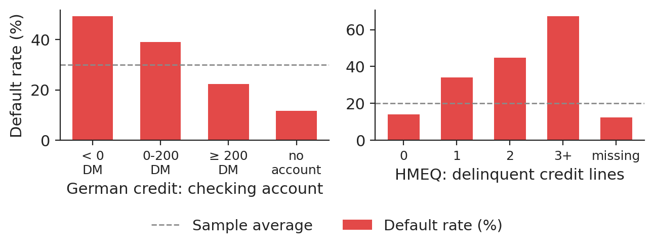
The simplest risk model is the default rate per group, \(\widehat{\mathrm{PD}}_g=\frac1{n_g}\sum_{i\in g}y_i\), where the probability of default (PD) of group \(g\) is the share of its loans with \(y_i=1\). In German credit, applicants with a negative checking balance default in 49.3 % of cases, those without a checking account in 11.7 %. In HMEQ, the rate climbs from 14.0 % with no delinquent credit line to 67.3 % with three or more.

Chart: Default rates differ strongly across simple applicant groups

Default rate by checking-account status (German credit) and by number of delinquent credit lines (HMEQ); dashed: sample average.

Source: UCI Statlog German credit; Baesens, Roesch and Scheule (2016), HMEQ. Data: 1,000 applicants (German credit); 5,960 loans (HMEQ).

In practice: a model must at least reproduce these group rates on the validation set.

Learning as minimisation of the average training loss, evaluated on new data

Slide 10 in the PDF

Training minimises the empirical risk \(\hat R_n(\boldsymbol\theta)=\frac1n\sum_i\ell(y_i,f(\mathbf x_i;\boldsymbol\theta))\), but the bank pays the risk on future applicants, \(R(\boldsymbol\theta)=\mathbb E\,\ell(y,f(\mathbf x;\boldsymbol\theta))\). We therefore split the data in three: training (\(\boldsymbol\theta\)), validation (model choice and stopping) and test (reported once). For HMEQ the stratified split gives 3,576, 1,192 and 1,192 loans; medians and scaling are fitted on the training part only, so no information leaks from the test set.

Section summary

Deep learning creates most value on raw, high-dimensional inputs; on small engineered tables it must beat logistic regression and boosting under a fixed protocol, on data that stay real from the first table to the last test.

Linear models are one-neuron networks

Linear and logistic regression are a single neuron with an identity or a sigmoid output; their losses are likelihoods and their gradients have the form that backpropagation will repeat in every layer.

Linear regression is one neuron with no activation

Slide 12 in the PDF

A neuron without activation computes \(\hat y=\mathbf w^\top\mathbf x+b\). With Gaussian errors, maximising the likelihood is the same as minimising the mean squared error (MSE), \(\frac1n\sum(y_i-\mathbf w^\top\mathbf x_i-b)^2\), which has the closed form \(\hat{\mathbf w}=(\mathbf X^\top\mathbf X)^{-1}\mathbf X^\top\mathbf y\). Networks lose this closed form and are trained by gradient descent (Lecture 2).

Logistic regression is one neuron with a sigmoid

Slide 13 in the PDF

With a sigmoid output, \(p_i=\sigma(\mathbf w^\top\mathbf x_i+b)\), and the Bernoulli negative log-likelihood (cross-entropy) as loss, the neuron is logistic regression:

\[\mathcal L(\mathbf w,b)=-\frac1n\sum_{i=1}^n\big[y_i\log p_i+(1-y_i)\log(1-p_i)\big],\qquad \nabla_{\mathbf w}\mathcal L=\frac1n\sum_{i=1}^n(p_i-y_i)\,\mathbf x_i\]
(1.1)

The gradient (1.1) is the error times the input; the loss is convex, so there is a single minimum, and \(e^{w_j}\) is the odds ratio of input \(j\).

Delinquencies and a missing debt ratio raise the odds of default most

Slide 14 in the PDF

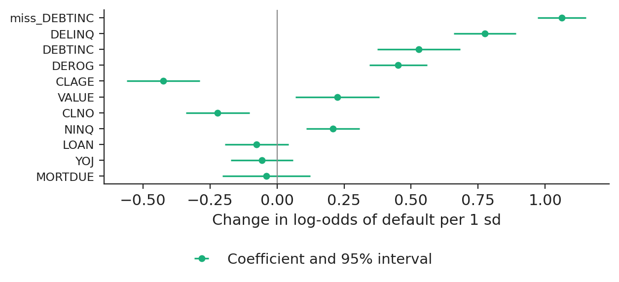
With standardised inputs, the coefficients are changes in log-odds per standard deviation and can be compared. The odds ratios are 2.89 for a missing debt-to-income ratio, 2.17 for more delinquent lines and 0.65 for an older credit history; McFadden's pseudo-\(R^2\) is 0.374.

Chart: Delinquencies and a missing debt ratio raise the odds of default most

Logistic regression on HMEQ: standardised coefficients with 95 % confidence intervals.

Source: Baesens, Roesch and Scheule (2016), HMEQ data. Data: 3,576 training loans.

In practice: a sign against credit sense is a reason to inspect the data, not to drop the model.

The forward pass of one real applicant, step by step

Slide 15 in the PDF

For one test applicant who later defaulted (a loan of 15,400 USD, debt-to-income 36.4 %, 2 delinquent lines), the score is the sum of the contributions \(w_jx_j\) plus the bias, \(z=\) −1.71, and the neuron outputs \(p=\sigma(z)=\) 15.3 %. The applicant would pass a 50 % cut-off; Section 5 shows why the cut-off should be set from costs.

Missing values as predictors of default

Slide 16 in the PDF

The debt-to-income ratio is missing for 21.3 % of HMEQ loans, and these default in 62.0 % of cases against 8.6 % when it is reported. Dropping incomplete rows would drop the riskiest applicants. We fill each numeric input with its training median and add an indicator of missingness, which gives \(d=\) 28 inputs.

In practice: never drop rows with missing values in credit data.

Section summary

One neuron with the right output and loss is a classical statistical model; the network view adds nothing yet, but it fixes the notation and the gradient that every deeper model reuses.

The perceptron

Rosenblatt's perceptron learns a linear boundary from its mistakes. It converges when the classes are separable and fails otherwise, which is the usual case in credit, and it cannot represent XOR.

From the McCulloch–Pitts neuron to the perceptron

Slide 18 in the PDF

McCulloch and Pitts (1943) wrote the neuron as a threshold unit, \(\hat y=\operatorname{step}(\mathbf w^\top\mathbf x+b)\); Rosenblatt (1958) made its weights learn from labelled examples. Minsky and Papert (1969) proved that one layer cannot represent XOR, and the field recovered only when backpropagation trained several layers (Rumelhart, Hinton and Williams, 1986).

The perceptron updates its weights only on misclassified examples

Slide 19 in the PDF

If example \(i\) is misclassified, \(y_i(\mathbf w^\top\mathbf x_i+b)\le0\) with \(y_i\in\{-1,+1\}\), the weights move towards it: \(\mathbf w\leftarrow\mathbf w+\eta y_i\mathbf x_i\). This is one step of stochastic gradient descent (SGD) on the perceptron criterion. Correct examples give no gradient and the output is a class, not a probability, which a lender cannot price.

If the classes can be separated, the perceptron stops after finitely many mistakes

Slide 20 in the PDF

Novikoff (1962): if a unit vector \(\mathbf w^*\) separates the data with margin \(\gamma\) and all inputs lie within radius \(R\), the perceptron makes at most \((R/\gamma)^2\) mistakes, whatever the number of examples or the dimension. Without a separating hyperplane the theorem says nothing.

The perceptron does not converge on non-separable credit data

Slide 21 in the PDF

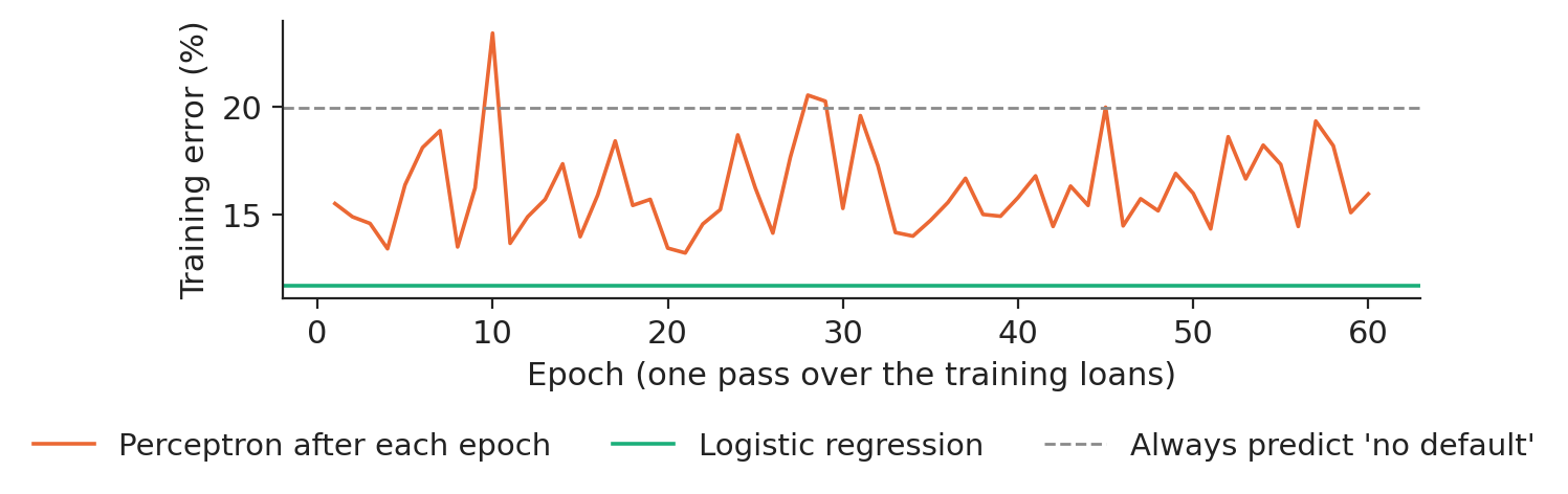
On the HMEQ training loans the classes overlap. Over 60 epochs the training error jumps between 13.2 % and 23.4 % after 35,876 updates, while logistic regression on the same inputs reaches 11.7 % and always predicting 'no default' 19.9 %.

Chart: The perceptron does not converge on non-separable credit data

Training error of the perceptron after each epoch on HMEQ, against logistic regression and the majority rule.

Source: Baesens, Roesch and Scheule (2016), HMEQ data. Data: 3,576 training loans.

In practice: a smooth loss and a probability output fix both problems.

The XOR problem and the hidden layer

Slide 22 in the PDF

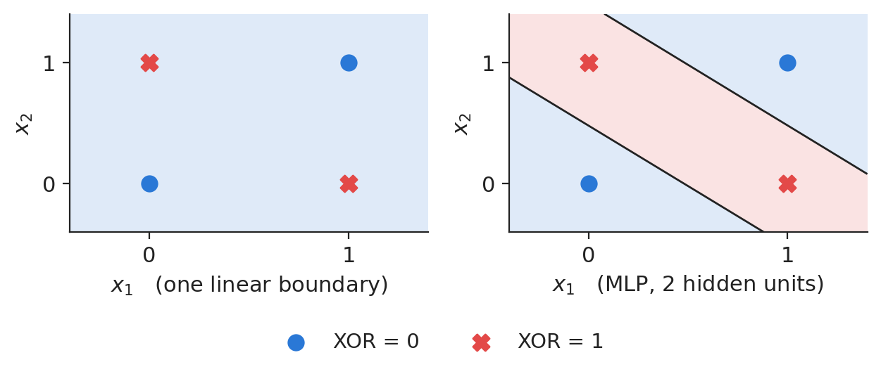
XOR is true when exactly one input is on. Any linear boundary classifies at most three of the four points correctly (50 % here), while an MLP with two tanh hidden units reaches 100 %: the hidden layer maps the inputs to a space where the classes become separable. Interactions such as 'high debt and short history' are of this kind. This is a mechanism picture on the logical table, not a data result.

Chart: The XOR problem and the hidden layer

XOR: one linear boundary (left) and an MLP with two hidden units (right).

Source: logical XOR table (no data). Data: the four XOR inputs.

Section summary

The perceptron is a linear classifier that learns only from mistakes; it converges on separable data and cycles on real, overlapping classes. Smooth losses, probability outputs and hidden layers remove these limits.

The multilayer perceptron

Stacking affine maps and nonlinear activations gives the MLP: we write its forward pass, choose activations and outputs, count parameters, and see what the universal approximation theorem does and does not promise.

An MLP alternates affine maps and nonlinear activations

Slide 24 in the PDF

Each hidden layer computes \(\mathbf h^{(l)}=a(\mathbf W^{(l)}\mathbf h^{(l-1)}+\mathbf b^{(l)})\), starting from \(\mathbf h^{(0)}=\mathbf x\), and the output layer is a logistic regression on the last hidden features. Without the activation \(a\) the layers collapse into one linear map. Our credit network has \(d=\) 28 inputs and two hidden layers of 64 rectified linear units (ReLU).

Activation functions and their properties

Slide 25 in the PDF

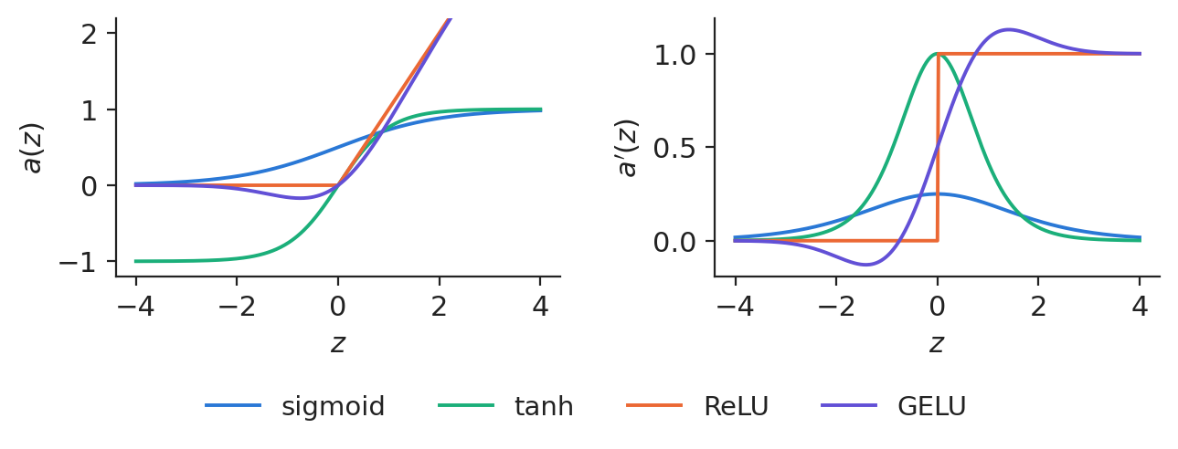
Sigmoid and tanh saturate: the derivative of the sigmoid is at most 0.25 and both derivatives vanish for large inputs, which slows learning in deep networks (Lecture 2). ReLU, \(\max(0,z)\), has slope 1 for positive inputs and is the default in hidden layers; the Gaussian error linear unit (GELU), \(z\Phi(z)\), is its smooth variant used in transformers.

Chart: Activation functions and their properties

Activation functions (left) and their derivatives (right); analytic curves.

Source: analytic functions (no data). Data: functions plotted on [-4, 4].

The output layer and the loss come from the type of the target

Slide 26 in the PDF

The output and the loss follow from the distribution of the target: identity and MSE for a real number, sigmoid and cross-entropy for a binary event, softmax and categorical cross-entropy for \(K\) classes, and the pinball loss for a quantile, such as the value at risk (VaR) of Lecture 2. Each pair is a maximum-likelihood estimator.

A small MLP already has hundreds of times more parameters than the logistic score

Slide 27 in the PDF

The number of parameters is \(\sum_l(H_{l-1}+1)H_l\). On HMEQ the logistic model has 29 parameters and the MLP 64-64 has 6,081, for 3,576 training loans: enough to memorise the training defaults, which is why every network keeps the weights of its best validation epoch.

One hidden layer can approximate any continuous function

Slide 28 in the PDF

For any continuous function on a compact set and any tolerance, a one-hidden-layer network with enough units approximates it (Cybenko, 1989; Hornik, 1991). The theorem does not say how many units are needed, whether gradient descent finds the weights, or whether they generalise.

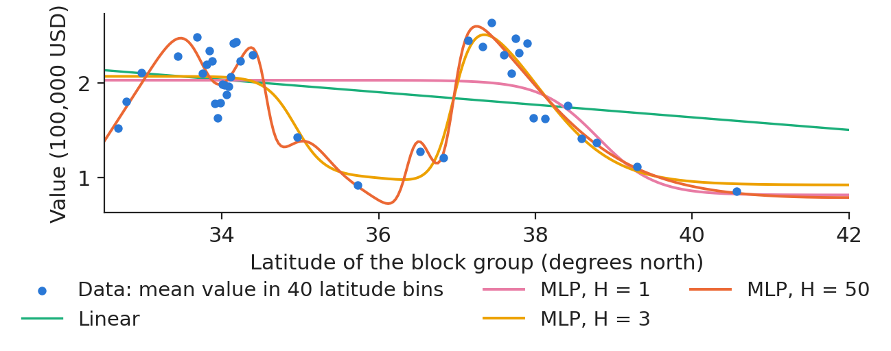
More hidden units trace the price geography of California

Slide 29 in the PDF

House values in California peak around Los Angeles and San Francisco. Fitting them on latitude alone, the held-out MSE falls from 0.896 for a straight line to 0.855, 0.757 and 0.731 with 1, 3 and 50 sigmoid units. The 992 block groups at the source cap of 500,000 USD are left out.

Chart: More hidden units trace the price geography of California

House values against latitude: bin means and fitted networks with 1, 3 and 50 hidden units.

Source: StatLib, California housing, 1990 census (Pace and Barry, 1997). Data: 19,648 block groups below the source cap.

In practice: location effects are nonlinear: a linear term cannot price them.

Depth and width of a network

Slide 30 in the PDF

A ReLU network is piecewise linear, and the number of its linear regions can grow exponentially with depth for a fixed number of units (Montúfar et al., 2014). On tabular credit data, two or three hidden layers are usually enough; depth pays off on images, text and sequences.

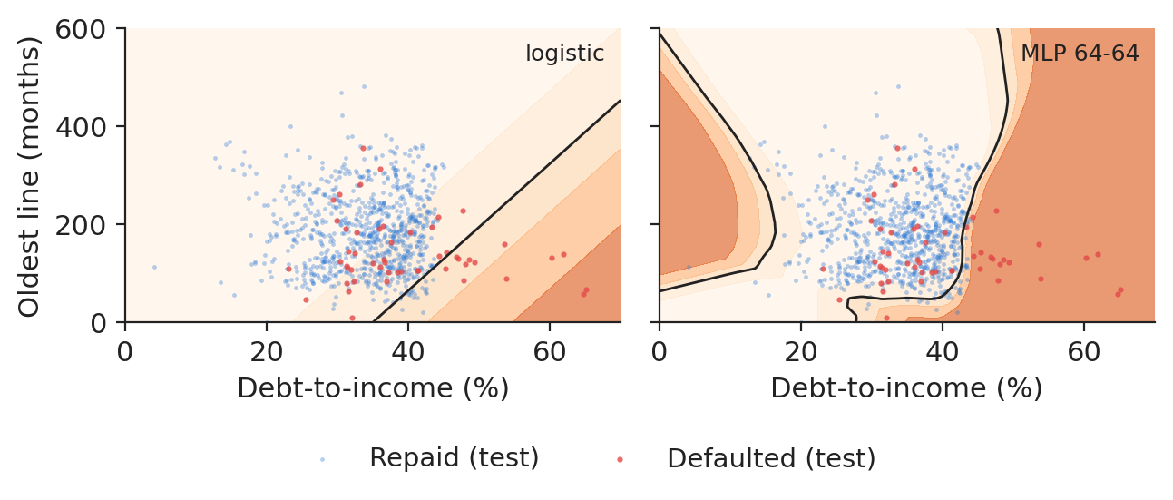
Nonlinear decision boundary of an MLP with two inputs

Slide 31 in the PDF

With two HMEQ inputs, debt-to-income and the age of the oldest credit line, the logistic model draws straight probability bands and the MLP curved regions. The area under the receiver operating characteristic (ROC) curve (AUC), the probability that a random defaulter scores above a random good loan, is 0.744 for the logistic model and 0.736 for the MLP: flexibility does not help when the two inputs carry little extra signal.

Chart: Nonlinear decision boundary of an MLP with two inputs

Predicted PD on two HMEQ variables: logistic regression (left) and MLP 64-64 (right), with test loans.

Source: Baesens, Roesch and Scheule (2016), HMEQ data. Data: 2,708 training and 871 test loans with both variables.

Section summary

An MLP is a stack of affine maps and activations; ReLU in the hidden layers, an output and loss that match the target, and a parameter count that tells how much data and regularisation are needed.

Case study: credit scoring with real loans

Logistic regression, an MLP and extreme gradient boosting (XGBoost) are compared on HMEQ and German credit with the same splits, inputs and metrics, several seeds, bootstrap intervals, a corrected test, calibration and the cost of errors.

Experimental protocol: a common split and common inputs for three models

Slide 33 in the PDF

The MLPs use ReLU layers, Adam with learning rate 0.001 and the weights of the best validation epoch, each with 5 seeds; XGBoost uses depth 4, learning rate 0.03 and early stopping on validation. HMEQ has one stratified 60/20/20 split; German credit uses 5 times repeated 5-fold cross-validation (25 test folds). All models trained on the central processing unit (CPU) with seed 20261108.

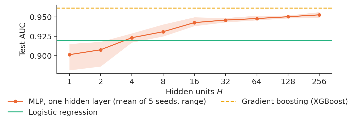
On HMEQ, a wider hidden layer raises the test AUC above the logistic score

Slide 34 in the PDF

With one hidden layer, the test AUC rises from 0.901 with one unit, essentially a logistic model, to 0.953 with 256 units; logistic regression reaches 0.920 and XGBoost 0.961. The gain flattens after about 16 units and the seed spread shrinks as the network widens.

Chart: On HMEQ, a wider hidden layer raises the test AUC above the logistic score

Test AUC on HMEQ against the number of hidden units (mean and range of 5 seeds), with the two benchmarks.

Source: Baesens, Roesch and Scheule (2016), HMEQ data. Data: 3,576 training, 1,192 validation, 1,192 test loans.

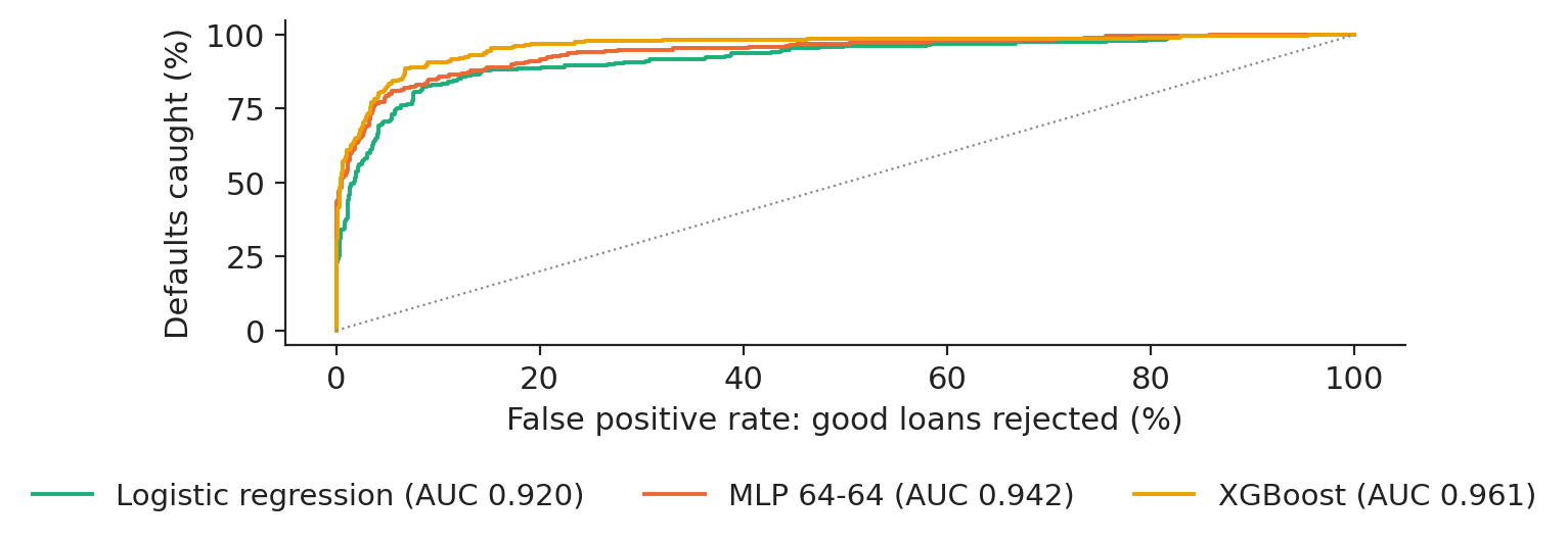
At a 10 % false-alarm rate, the MLP catches more defaults than the logistic score

Slide 35 in the PDF

The ROC curve plots the share of defaults caught against the share of good loans rejected for every cut-off. When 10 % of good loans are rejected, logistic regression catches 83.2 % of the 238 test defaults, the MLP 85.3 % and XGBoost 90.8 %.

Chart: At a 10 % false-alarm rate, the MLP catches more defaults than the logistic score

ROC curves on the HMEQ test set.

Source: Baesens, Roesch and Scheule (2016), HMEQ data. Data: 1,192 test loans (238 defaults).

In practice: read the curve at the rejection rate the business accepts.

The MLP gain on HMEQ is larger than seed noise and test-set noise

Slide 36 in the PDF

The MLP 64-64 reaches a mean test AUC of 0.945 over 5 seeds (standard deviation 0.004). A paired bootstrap of the test loans gives the AUC gain over logistic regression, 0.023, a 95 % interval of [0.008; 0.037], which excludes zero.

The scores are close to calibrated probabilities

Slide 37 in the PDF

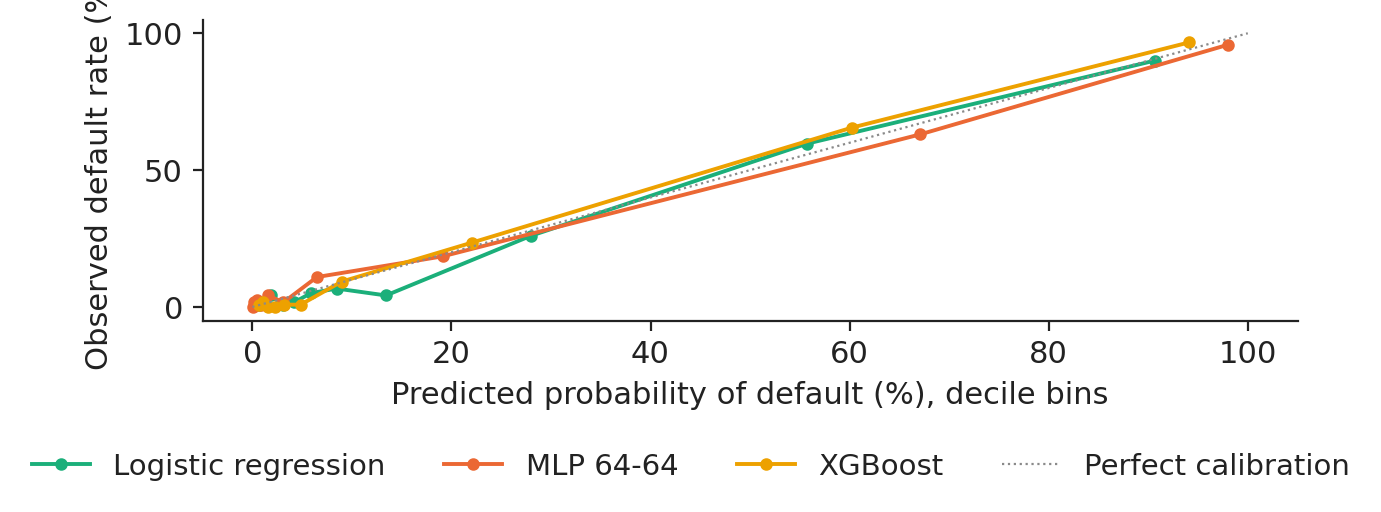
Provisions and loan prices use the PD itself, so the probabilities must be right in level, not only in order. In each decile of predicted PD the observed default rate is close to the predicted one; the Brier scores are 0.0742 for logistic regression, 0.0625 for the MLP and 0.0549 for XGBoost, against 0.1598 for a constant rate.

Chart: The scores are close to calibrated probabilities

Reliability diagram on the HMEQ test set: predicted against observed default rate by decile.

Source: Baesens, Roesch and Scheule (2016), HMEQ data. Data: 1,192 test loans.

On 1,000 German applicants, the MLP does not beat logistic regression

Slide 38 in the PDF

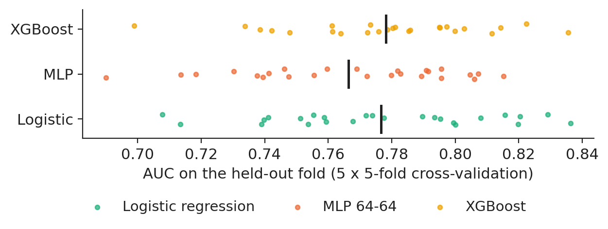
On German credit the picture changes: mean AUC 0.777 for logistic regression, 0.766 for the MLP and 0.778 for XGBoost across 25 held-out folds. With so few applicants the network has nothing to add.

Chart: On 1,000 German applicants, the MLP does not beat logistic regression

AUC of each held-out fold in 5 x 5-fold cross-validation on German credit; bars are means.

Source: UCI Machine Learning Repository, Statlog German credit. Data: 1,000 applicants, 25 held-out folds.

Why the usual t-test overstates differences in cross-validation

Slide 39 in the PDF

The fold scores are correlated because the training sets overlap, so the naive t-test is too optimistic. The Nadeau-Bengio correction inflates the variance by \(1/J+n_{\text{test}}/n_{\text{train}}\); the MLP against logistic regression gives \(t=\) −0.93 and \(p=\) 0.362, so there is no evidence of a difference.

Cost-sensitive cut-off of 1/6 when a missed default costs five times a rejected good applicant

Slide 40 in the PDF

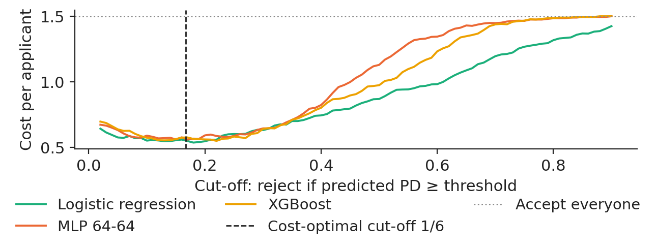
The UCI cost matrix weighs a missed bad risk 5 times a rejected good applicant. Rejecting when \(5p\ge1-p\) gives the cut-off \(1/6\). With out-of-fold predictions, the logistic model costs 0.554 per applicant at 1/6 and 0.870 at 1/2; the MLP 0.568 and 1.130; accepting everyone costs 1.50.

Chart: Cost-sensitive cut-off of 1/6 when a missed default costs five times a rejected good applicant

Cost per German credit applicant against the cut-off, out-of-fold predictions; dashed: cut-off 1/6.

Source: UCI Machine Learning Repository, Statlog German credit. Data: 1,000 applicants, out-of-fold predictions.

In practice: the cut-off is where most money is lost or saved.

A minimal MLP implementation in PyTorch

Slide 41 in the PDF

Fifteen lines are enough: an `nn.Sequential` of linear layers and ReLUs, `BCEWithLogitsLoss` (sigmoid and cross-entropy in one stable function), the Adam optimiser and a loop of `zero_grad`, `backward` and `step`. The notebook of this lecture adds the data pipeline, the validation stopping and the seeds.

Explore it visually

Free interactive tools and illustrated guides for this lecture; most run in the browser.

  • TensorFlow Playground: choose the circle data set and keep only the inputs \(x_1, x_2\). With no hidden layer the boundary stays a straight line, as in logistic regression; add one hidden layer of four neurons and the boundary closes around the circle.
  • TensorFlow Playground: keep the hidden layer and set the activation to Linear: the boundary is straight again, because a composition of linear maps is linear.
  • 3Blue1Brown, chapter 1: what the weights, biases and layers of a network compute, on handwritten digits.

Section summary

On 3,576 HMEQ loans the MLP beats the logistic score (AUC 0.945 against 0.920) and boosting beats both; on 1,000 German applicants nothing beats logistic regression significantly. In both cases the cost-based cut-off matters more than the model.

Videos: the intuition behind the mathematics (in English)

Abbreviations

AIartificial intelligence
AUCarea under the receiver operating characteristic curve
CPUcentral processing unit
DMDeutsche Mark
ESexpected shortfall
GELUGaussian error linear unit
GNNgraph neural network
GPUgraphics processing unit
GraphSAGEgraph sample and aggregate (a GNN architecture)
HMEQhome equity loans dataset
ICBEInternational Conference on Business Excellence
IEEE-CISInstitute of Electrical and Electronics Engineers, Computational Intelligence Society
LLMlarge language model
MLPmultilayer perceptron
MSEmean squared error
PDprobability of default
ReLUrectified linear unit
ROCreceiver operating characteristic
SGDstochastic gradient descent
SHAPShapley additive explanations
UCIUniversity of California, Irvine (Machine Learning Repository)
USDUS dollar
VaRvalue at risk
VLMvision-language model
XAIexplainable artificial intelligence
XGBoostextreme gradient boosting
XORexclusive or

References

  • Bishop, C. M. & Bishop, H. (2024). Deep Learning: Foundations and Concepts. Springer. doi:10.1007/978-3-031-45468-4
  • Baesens, B., Rösch, D. & Scheule, H. (2016). Credit Risk Analytics. Wiley. doi:10.1002/9781119449560
  • Będowska-Sójka, B., Wójcik, P. & Pele, D. T. (2026). Early warning systems for cryptocurrency markets: Predicting `zombie' assets using machine learning. The North American Journal of Economics and Finance, 81, 102543. doi:10.1016/j.najef.2025.102543
  • Chen, T. & Guestrin, C. (2016). XGBoost: A scalable tree boosting system. Proceedings of KDD 2016, 785–794. doi:10.1145/2939672.2939785
  • Cybenko, G. (1989). Approximation by superpositions of a sigmoidal function. Mathematics of Control, Signals and Systems, 2(4), 303–314. doi:10.1007/BF02551274
  • Diaconu, D. & Pele, D. T. (2026). Explainable AI in financial fraud detection: Evidence from the IEEE-CIS fraud dataset. Proceedings of the International Conference on Business Excellence, 20(1), 118–132. doi:10.2478/picbe-2026-0015
  • Grinsztajn, L., Oyallon, E. & Varoquaux, G. (2022). Why do tree-based models still outperform deep learning on typical tabular data? Advances in Neural Information Processing Systems, 35. arXiv:2207.08815
  • Hofmann, H. (1994). Statlog (German Credit Data). UCI Machine Learning Repository. doi:10.24432/C5NC77
  • Hornik, K. (1991). Approximation capabilities of multilayer feedforward networks. Neural Networks, 4(2), 251–257. doi:10.1016/0893-6080(91)90009-T
  • Jheng, S.-L., Pele, D. T., Tak, R. & Găman, Ș. (2026). A multimodal vision-language framework for financial anomaly detection. Proceedings of the International Conference on Business Excellence, 20(1), 191–201. doi:10.2478/picbe-2026-0020
  • Jheng, S.-L., Tak, R., Găman, Ș., Mazurencu-Marinescu-Pele, M. & Pele, D. T. (2026). Can foundation models manage risk? Zero-shot VaR and ES forecasting with conformal calibration in CEE markets. Economic Computation and Economic Cybernetics Studies and Research, 60(2), 267–290. doi:10.24818/18423264/60.2.26.14
  • LeCun, Y., Bengio, Y. & Hinton, G. (2015). Deep learning. Nature, 521, 436–444. doi:10.1038/nature14539
  • Lessmann, S., Baesens, B., Seow, H.-V. & Thomas, L. C. (2015). Benchmarking state-of-the-art classification algorithms for credit scoring: An update of research. European Journal of Operational Research, 247(1), 124–136. doi:10.1016/j.ejor.2015.05.030
  • McCulloch, W. S. & Pitts, W. (1943). A logical calculus of the ideas immanent in nervous activity. The Bulletin of Mathematical Biophysics, 5(4), 115–133. doi:10.1007/BF02478259
  • Minsky, M. & Papert, S. (1969). Perceptrons: An Introduction to Computational Geometry. MIT Press.
  • Nadeau, C. & Bengio, Y. (2003). Inference for the generalization error. Machine Learning, 52(3), 239–281. doi:10.1023/A:1024068626366
  • Novikoff, A. B. J. (1962). On convergence proofs on perceptrons. Proceedings of the Symposium on the Mathematical Theory of Automata, 12, 615–622. Polytechnic Institute of Brooklyn.
  • Pace, R. K. & Barry, R. (1997). Sparse spatial autoregressions. Statistics & Probability Letters, 33(3), 291–297. doi:10.1016/S0167-7152(96)00140-X
  • Montúfar, G., Pascanu, R., Cho, K. & Bengio, Y. (2014). On the number of linear regions of deep neural networks. Advances in Neural Information Processing Systems, 27. arXiv:1402.1869
  • Paszke, A. et al. (2019). PyTorch: An imperative style, high-performance deep learning library. Advances in Neural Information Processing Systems, 32. arXiv:1912.01703
  • Pele, D. T., Bolovăneanu, V., Lin, M.-B., Ren, R., Ginavar, A. T., Spilak, B., Andrei, A.-V., Toma, F.-M., Lessmann, S. & Härdle, W. K. (2026). In the beginning was the Word: LLM-VaR and LLM-ES. Expert Systems with Applications, 295, 128676. doi:10.1016/j.eswa.2025.128676
  • Rosenblatt, F. (1958). The perceptron: A probabilistic model for information storage and organization in the brain. Psychological Review, 65(6), 386–408. doi:10.1037/h0042519
  • Rumelhart, D. E., Hinton, G. E. & Williams, R. J. (1986). Learning representations by back-propagating errors. Nature, 323, 533–536. doi:10.1038/323533a0

Text written for the web version of the lecture; numbers, charts and sources come from the slides and their Quantlets.