Neural Networks and Deep Learning

Lecture 10: Reinforcement learning: trading, hedging and battery dispatch

Lecture 10

Reinforcement learning: trading, hedging and battery dispatch

Prof. dr. Daniel Traian PELE

Bucharest University of Economic Studies (ASE), Department of Statistics and Econometrics
Romanian Academy, Institute for Economic Forecasting (IPE)

Some business decisions change the situation in which the next decision is taken. A battery that charges now cannot charge again in an hour; a trader who sells today pays a cost to buy back tomorrow; a desk that hedges an option adjusts the hedge every day. Reinforcement learning (RL) is the branch of machine learning built for such sequential decisions: an agent observes a state, takes an action, receives a reward and moves to a new state, and it learns a policy that maximises the total reward.

This lecture writes three real business problems in that language and solves them on real data. The first is the dispatch of a 2 MWh battery on Romanian day-ahead prices, solved exactly by dynamic programming (DP) and then learned by tabular Q-learning and a deep Q-network (DQN). The second is trading the S&P 500 with proximal policy optimisation (PPO), an actor-critic method. The third is hedging a one-month option with a neural policy that minimises the expected shortfall (ES) of the loss. Every agent is trained with five seeds and compared with the rule a practitioner already uses. The verdict is mixed, and instructive: the simple rule wins for the battery, PPO's advantage in trading is not statistically established, and the learned hedge beats the textbook delta in every seed.

What you will be able to do

  • Write a business decision as a Markov decision process (MDP): state, action, reward, transition and discount.
  • Solve a small MDP exactly with the Bellman equation and dynamic programming, and read the value function.
  • Train value-based agents (Q-learning, DQN) and a policy-gradient agent (PPO) on real prices, with several seeds and an honest benchmark.
  • Hedge an option with a neural policy that minimises the expected shortfall of the loss, and compare it with the Black-Scholes delta.
  • Judge when RL adds value in business and when a simple rule is enough.

Lecture plan

  1. Sequential decisions in businessReinforcement learning is about what to do, not about what will happen.
  2. Markov decision processes and the Bellman equationAn MDP formalises a sequential decision; the Bellman equation breaks it into one-step problems that dynamic programming solves exactly when the model is known.
  3. Value-based learning: Q-learning and DQNQ-learning and the deep Q-network learn \(Q^*\) from samples, without knowing the day's prices in advance.
  4. Policy gradients and PPO: trading the S&P 500Policy-gradient methods parameterise the policy directly.
  5. Deep hedging: a policy that minimises tail riskDeep hedging (Buehler et al., 2019) trains a neural hedging policy on the risk measure the desk reports.

Sequential decisions in business

Reinforcement learning is about what to do, not about what will happen. This section sets up the agent-environment loop and the three problems of the lecture.

Reinforcement learning and supervised learning

Slide 6 in the PDF

Supervised learning has a label for every example, and its predictions do not change the next example. In reinforcement learning the agent sees a state \(s_t\), chooses an action \(a_t\) and receives a reward \(r_{t+1}\); the action changes the next state, and no teacher says what the right action was, only how much reward followed. Storage, trading, hedging, inventory, pricing and credit limits all have this structure. When today's action does not change tomorrow's options, a forecast and a rule are enough.

In practice: use RL only when today's action changes tomorrow's options.
The agent-environment loop

Slide 7 in the PDF

The agent follows a policy \(\pi_\theta(a\mid s)\); the environment answers each action with a reward and a new state. An episode is one delivery day for the battery, a window of 126 trading days for the trader and the 21-day life of an option for the hedger. All three agents are model-free (they learn from sampled transitions \((s_t,a_t,r_{t+1},s_{t+1})\), never from the law of the market) and offline (they learn from historical data).

In practice: write down state, action and reward before training anything.

Three business applications of reinforcement learning

Slide 8 in the PDF
ProblemState \(s_t\)Action \(a_t\)Reward \(r_{t+1}\)
Batteryhour, stored energy, yesterday's pricescharge / idle / dischargecash flow of the hour (EUR)
Tradingpast returns, volatility, VIX, trend, current positionflat / longposition × next return − cost
Hedgingindex level, time to maturity, VIX, previous hedgehedge ratio in [0, 1]final profit and loss, judged by its ES

The data are real: hourly day-ahead prices for Romania (RO), Hungary (HU), Germany–Luxembourg (DE-LU) and Bulgaria (BG) from energy-charts.info, the portal of the Fraunhofer Institute for Solar Energy Systems (ISE), based on data of the European Network of Transmission System Operators for Electricity (ENTSO-E); and daily closes of the S&P 500 and of the Cboe Volatility Index (VIX) from Yahoo Finance, up to 31 October 2026. Each problem is split in time order into training, validation and test periods. The benchmarks are rules a manager already uses: yesterday's optimal plan, buy-and-hold, the 200-day moving average and the Black-Scholes delta.

In practice: an RL agent is worth deploying only if it beats the rule the desk already uses, after costs and over several seeds.

Battery revenue from the daily price spread and the growth of the spread

Slide 9 in the PDF

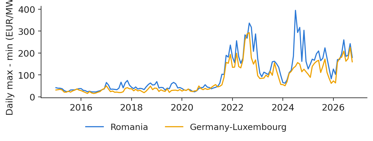
A battery buys in the cheapest hours and sells in the dearest, so its income depends on the daily spread between the maximum and minimum price, not on the price level. In Romania the mean daily spread was 47.9 EUR/MWh in 2019, 164.3 in 2025 and 182.8 in 2026 so far; the peak month was July 2024, at 394.4 EUR/MWh. Solar generation now pushes midday prices down, and evening peaks remain.

Chart: Battery revenue from the daily price spread and the growth of the spread

Monthly mean of the daily max–min spread of day-ahead prices in Romania and Germany–Luxembourg.

Source: energy-charts.info (Fraunhofer ISE), from exchange and ENTSO-E data. Data: 2 Jan 2015 to 31 Oct 2026, monthly mean of the daily spread.

In practice: the business case of a battery is a bet on future spreads, not on the price level.

Markov decision processes and the Bellman equation

An MDP formalises a sequential decision; the Bellman equation breaks it into one-step problems that dynamic programming solves exactly when the model is known.

The five elements of a Markov decision process

Slide 11 in the PDF

An MDP is \(\mathcal M=(\mathcal S,\mathcal A,P,R,\gamma)\): states, actions, transition law \(P(s'\mid s,a)\), expected reward \(R(s,a)\) and discount factor \(\gamma\in[0,1]\). The agent maximises the expected return

\[G_t=\sum_{k=0}^{T-t-1}\gamma^{k}r_{t+k+1},\qquad \pi^{*}=\arg\max_{\pi}\mathbb E_{\pi}[G_0]\]
(10.1)

The Markov property requires the state to contain everything relevant: for the battery, the hour and the stored energy; for the trader, the current position, because it determines the cost of the next trade. The battery episodes last 24 steps and use \(\gamma=1\); trading uses \(\gamma=0.99\).

In practice: a missing state variable, such as the current position, makes the agent erratic.

Value functions measure how good a state is

Slide 12 in the PDF

The state value \(V^{\pi}(s)=\mathbb E_\pi[G_t\mid s_t=s]\) is the expected future reward from a state; the action value \(Q^{\pi}(s,a)\) is the same after a given first action, and the advantage \(A^{\pi}(s,a)=Q^{\pi}(s,a)-V^{\pi}(s)\) compares an action with the policy's average. Value-based methods (Q-learning, DQN) estimate \(Q^*\) and act greedily; policy-based methods (REINFORCE, PPO) parameterise the policy directly and use \(V\) only as a baseline. For the battery, \(V_h(s)\) is the number of euros still to be earned today from hour \(h\) with \(s\) MWh stored.

The Bellman equation: recursive decomposition of the value function

Slide 13 in the PDF

The best value now is the best immediate reward plus the discounted best value of the next state:

\[V^{*}(s)=\max_{a}\Big\{R(s,a)+\gamma\sum_{s'}P(s'\mid s,a)\,V^{*}(s')\Big\},\qquad Q^{*}(s,a)=R(s,a)+\gamma\,\mathbb E_{s'}\big[\max_{a'}Q^{*}(s',a')\big]\]
(10.2)

For \(\gamma<1\) the right-hand side is a contraction, so value iteration converges to a unique fixed point; on a finite horizon one backward pass is exact (Bellman, 1957). Every algorithm of this lecture is an approximate way to solve this equation when the model is unknown or the state too large for a table.

The battery as an MDP

Slide 14 in the PDF

The state is the hour and the stored energy \(s_h\in\{0,1,2\}\) MWh; the action \(a_h\in\{-1,0,+1\}\) charges, idles or discharges one MWh of stored energy; the reward is the cash flow of the hour:

\[r_h(a_h)=\begin{cases}\eta_d\,p_h & a_h=+1\ \text{(sell)}\\ -p_h/\eta_c & a_h=-1\ \text{(buy)}\\ 0 & a_h=0\end{cases},\qquad s_{h+1}=s_h-a_h\]
(10.3)

where \(p_h\) is the day-ahead price of hour \(h\) and \(\eta_c=\eta_d=\sqrt{0.85}\), so a full cycle returns 85 % of the energy. The battery starts each day empty, cannot charge when full or discharge when empty (action masking), and is a price taker without degradation cost or grid fees. The data cover 4,292 Romanian delivery days with 24 complete hours, 2 January 2015 to 31 October 2026; since October 2025 each hour is the mean of four 15-minute prices.

In practice: the stored energy is what makes the decision sequential.

Dynamic programming solves the battery day exactly

Slide 15 in the PDF

Going backwards from midnight, with \(V_{24}(s)=0\),

\[V_h(s)=\max_{a:\,0\le s-a\le 2}\big\{r_h(a)+V_{h+1}(s-a)\big\},\qquad h=23,\dots,0\]
(10.4)

and the revenue of the day is \(V_0(0)\). All 4,292 days are solved in milliseconds. Because DP uses the day's 24 prices before they are known, its revenue is an upper bound for any real strategy. The naive benchmark computes yesterday's optimal plan and applies it today. Every learning agent is scored by its capture ratio, its revenue divided by the perfect-foresight revenue.

In practice: DP gives the ceiling against which every learning agent is scored.

Optimal battery schedule for one day

Slide 16 in the PDF

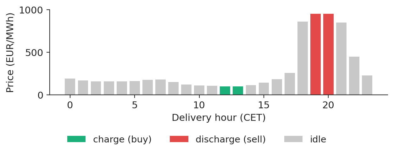
On 30 June 2026, the day of 2026 with the largest spread, prices ranged from 100.65 EUR/MWh at 13:00 to 954.59 EUR/MWh at 20:00. The optimal plan charges in the two cheapest hours around midday and discharges in two evening hours, earning 1,541 EUR.

Chart: Optimal battery schedule for one day

Hourly day-ahead prices in Romania on 30 June 2026, coloured by the optimal action of the battery.

Source: energy-charts.info (Fraunhofer ISE), from exchange and ENTSO-E data. Data: Romania, 30 Jun 2026, hourly day-ahead prices.

The value function prices stored energy hour by hour

Slide 17 in the PDF

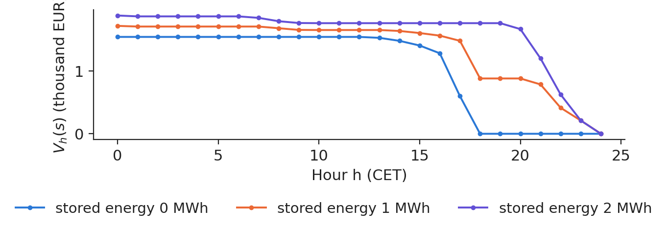
At 12:00 on the same day \(V_{12}(0)\) = 1,541 EUR and \(V_{12}(2)\) = 1,760 EUR: half of the difference, 109.38 EUR, is the value of one stored MWh, the shadow price of energy in the battery at noon. After the evening peak, stored energy is worth nothing. A good learned \(Q\) must reproduce this shape without seeing the day's prices.

Chart: The value function prices stored energy hour by hour

Value function \(V_h(s)\) of the battery problem on 30 June 2026 for 0, 1 and 2 MWh stored.

Source: energy-charts.info (Fraunhofer ISE), from exchange and ENTSO-E data. Data: Romania, 30 Jun 2026; own computation (backward induction).

Revenue of a 2 MWh battery under perfect foresight

Slide 18 in the PDF

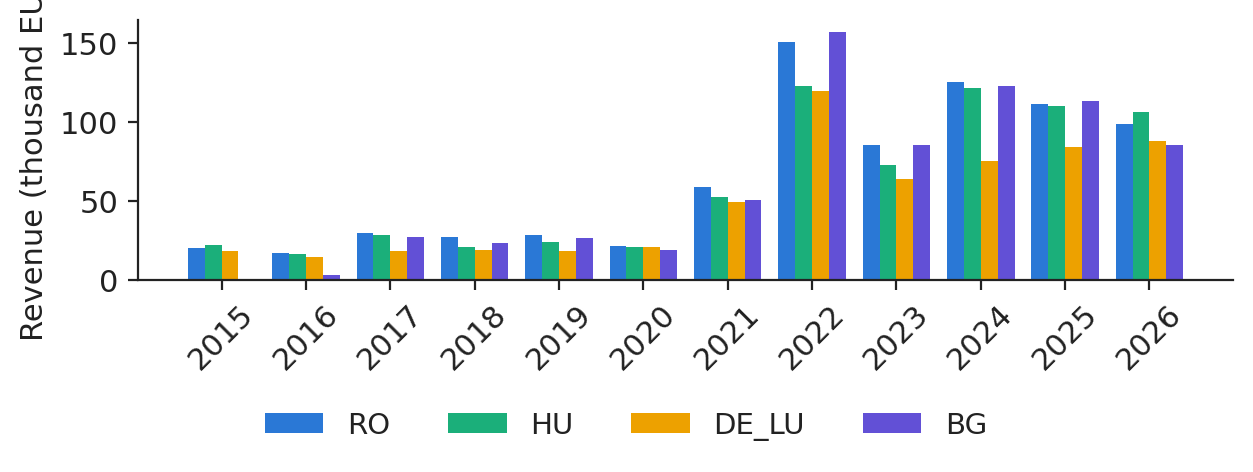
With perfect foresight the battery would have earned 28.4 thousand EUR in Romania in 2019, 150.2 in 2022, 111.2 in 2025 and 98.5 in January–October 2026 (302 days with 24 complete hours). In 2025 the same battery would have earned 109.9 thousand EUR in Hungary, 112.9 in Bulgaria and 84.3 in Germany–Luxembourg. These are ceilings: they follow the spreads, not the price level.

Chart: Revenue of a 2 MWh battery under perfect foresight

Perfect-foresight revenue of a 2 MWh battery by year and bidding zone (2026: January–October).

Source: energy-charts.info (Fraunhofer ISE), from exchange and ENTSO-E data. Data: 2015-2026 (*2026: January-October); days with 24 complete hours.

In practice: investors size storage on these numbers; a real operator captures only part of them.

Value-based learning: Q-learning and DQN

Q-learning and the deep Q-network learn \(Q^*\) from samples, without knowing the day's prices in advance.

Q-learning: learn Q* from samples, without a model

Slide 20 in the PDF

Q-learning (Watkins & Dayan, 1992) moves \(Q(s,a)\) towards the reward plus the best value of the next state:

\[Q(s_t,a_t)\leftarrow Q(s_t,a_t)+\alpha\big[r_{t+1}+\gamma\max_{a'}Q(s_{t+1},a')-Q(s_t,a_t)\big]\]
(10.5)

The bracket is the temporal-difference (TD) error, a learning signal available after every hour. The target uses the greedy action whatever the agent does next, so Q-learning is off-policy. It converges if every pair is visited infinitely often and the step sizes satisfy the Robbins–Monro conditions. Exploration is \(\varepsilon\)-greedy, with \(\varepsilon\) decayed from 1 to 0.05.

Definition of the state: information available to the agent

Slide 21 in the PDF

The operator plans before the day's prices are known, so the agent's state is \((h,\ \text{stored energy},\ q_h)\), where \(q_h\) is the quartile of hour \(h\) among yesterday's 24 prices: 288 states and 3 actions. The agent is trained on 1,746 days of 2019–2023 for 40 passes; the epoch with the best revenue on the 2024 validation year is kept, and the 638 test days, 1 January 2025 to 24 October 2026, are used once.

In practice: a state that leaks today's prices would give a perfect but useless backtest.

The policy learned by tabular Q-learning

Slide 22 in the PDF

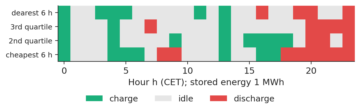
With one MWh stored, the agent mostly charges in the early-afternoon solar trough and discharges in the evening; yesterday's ranking shifts the timing. The table can be printed and audited hour by hour, which is an advantage of tabular methods.

Chart: The policy learned by tabular Q-learning

Action of the tabular Q-learning agent with 1 MWh stored, by hour and by yesterday's price quartile of that hour (first seed).

Source: energy-charts.info (Fraunhofer ISE), from exchange and ENTSO-E data. Data: rows = quartile of the hour's price yesterday; seed 20261108.

The deep Q-network: a neural approximation of the Q-table

Slide 23 in the PDF

The DQN replaces the table by a network \(Q_\theta(s,a)\) and regresses it on the TD target (Mnih et al., 2015). Double DQN lets the online network choose the next action and a slowly updated target network evaluate it, which removes the upward bias of a maximum over noisy estimates (van Hasselt, Guez & Silver, 2016):

\[y=r+\gamma\,Q_{\theta^{-}}\big(s',\arg\max_{a'}Q_{\theta}(s',a')\big),\qquad \mathcal L(\theta)=\mathbb E\big[\ell_{\text{Huber}}(y-Q_\theta(s,a))\big]\]
(10.6)

Our network has 82 inputs (yesterday's and last week's 24 standardised prices, the weekday, the hour and the stored energy) and two layers of 128 rectified linear units (ReLU). A replay memory of the last four epochs breaks the correlation of consecutive hours.

Learning curves: validation revenue by training epoch

Slide 24 in the PDF

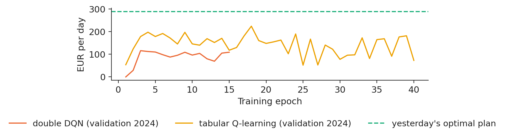
Both agents improve quickly, but on the 2024 validation year they stay below yesterday's optimal plan: the best validation revenue per day, averaged over five seeds, is 200 EUR for the DQN and 211 EUR for Q-learning, against 289 EUR for the naive plan.

Chart: Learning curves: validation revenue by training epoch

Validation revenue per day (2024) after each training epoch; line = mean, band = range over five seeds.

Source: energy-charts.info (Fraunhofer ISE), from exchange and ENTSO-E data. Data: validation year 2024; band = range over 5 seeds.

Share of the perfect-foresight revenue captured in the test years

Slide 25 in the PDF

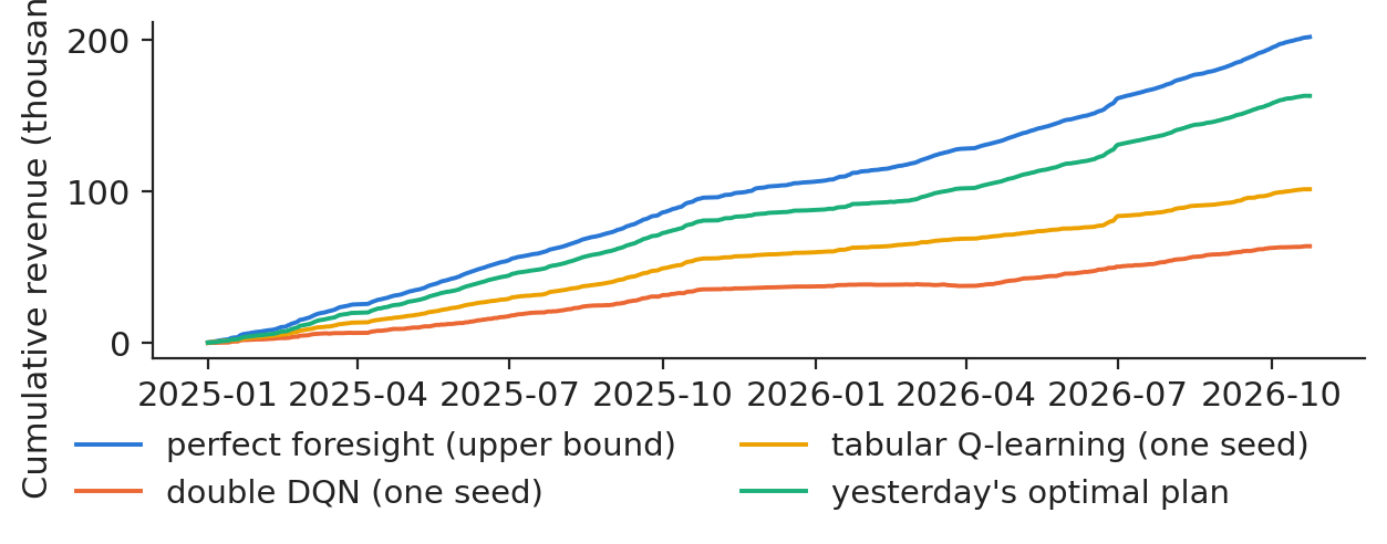
On the test days the perfect-foresight revenue is 202.1 thousand EUR. Yesterday's optimal plan earns 163.1, tabular Q-learning 115.2 and the double DQN 101.3 (means of five seeds).

Chart: Share of the perfect-foresight revenue captured in the test years

Cumulative revenue on the test days (2025 to October 2026): perfect foresight, the two learning agents and yesterday's optimal plan.

Source: energy-charts.info (Fraunhofer ISE), from exchange and ENTSO-E data. Data: 1 Jan 2025 to 24 Oct 2026 (test); trained on 2019-2023, validated on 2024.

Battery results on the test years, five seeds

Slide 26 in the PDF
StrategyRevenue (thousand EUR)Capture (%)Range over seeds (%)
Perfect foresight (upper bound)202.1100–
Double DQN101.350.143.9 – 58.5
Tabular Q-learning115.257.050.2 – 61.9
Yesterday's optimal plan163.180.7–

A Diebold–Mariano (DM) test on the daily revenue differences between the DQN and the naive plan, with a Newey–West variance, gives \(t=-18.99\): the DQN earns 96.8 EUR less per day, and neither agent beats the naive plan in any seed. The rule wins because it optimises on all 24 of yesterday's prices, while the agents learn one average policy from a compressed state. The lesson is not that RL fails, but that it must be benchmarked against the rule in use; richer states (a price forecast, the naive plan itself as an input) are the natural next step.

In practice: report the capture ratio with its range over seeds and a test against the naive plan, never a single best run.

Policy gradients and PPO: trading the S&P 500

Policy-gradient methods parameterise the policy directly. PPO is the most used of them.

Policy-gradient methods

Slide 28 in the PDF

The policy gradient theorem (Sutton et al., 2000) gives

\[\nabla_{\theta}J(\theta)=\mathbb E_{\pi_{\theta}}\Big[\sum_{t}\nabla_{\theta}\log\pi_{\theta}(a_t\mid s_t)\,\big(G_t-b(s_t)\big)\Big]\]
(10.7)

where \(b(s_t)\) is any function of the state, a baseline that leaves the gradient unbiased and lowers its variance. REINFORCE (Williams, 1992) uses the Monte Carlo return \(G_t\). The gradient needs no derivative of the transition law, so the market can remain a black box, and stochastic policies explore by themselves.

Actor-critic and the advantage estimate

Slide 29 in the PDF

A critic \(V_\phi\) predicts the return and the actor learns from the surprise. Generalised advantage estimation (GAE) (Schulman et al., 2016) averages TD errors \(\delta_t=r_{t+1}+\gamma V_\phi(s_{t+1})-V_\phi(s_t)\):

\[\hat A_t=\sum_{l\ge0}(\gamma\lambda)^{l}\,\delta_{t+l}\]
(10.8)

with \(\lambda=0\) giving the one-step TD advantage and \(\lambda=1\) the Monte Carlo advantage; we use \(\gamma=0.99\) and \(\lambda=0.95\). Actor and critic share two layers of 64 tanh units, and an entropy bonus of 0.01 keeps the policy from collapsing too early.

PPO: clipped policy updates

Slide 30 in the PDF

PPO (Schulman et al., 2017) maximises the clipped objective

\[\mathcal L^{\text{CLIP}}(\theta)=\mathbb E_t\big[\min\big(\rho_t\hat A_t,\ \mathrm{clip}(\rho_t,1-\epsilon,1+\epsilon)\hat A_t\big)\big],\qquad \rho_t=\frac{\pi_\theta(a_t\mid s_t)}{\pi_{\theta_{\text{old}}}(a_t\mid s_t)}\]
(10.9)

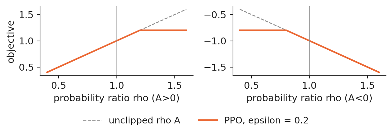
With \(\epsilon=0.2\), once the probability ratio leaves \([1-\epsilon,1+\epsilon]\) in the favourable direction, the gradient of that sample is zero: a cheap substitute for the Kullback–Leibler (KL) trust region of trust region policy optimisation (TRPO). The chart is an analytic illustration of the mechanism, not data.

Chart: PPO: clipped policy updates

The clipped surrogate objective as a function of the probability ratio, for a positive and a negative advantage (analytic function).

Source: Schulman et al. (2017), clipped surrogate objective. Data: analytic function, no data.

Trading as an MDP: flat or long the S&P 500

Slide 31 in the PDF

Each evening the agent chooses tomorrow's position \(a_t\in\{0,1\}\) and receives

\[r_{t+1}=a_t\ln\frac{P_{t+1}}{P_t}-c\,|a_t-a_{t-1}|,\qquad c=5\ \text{bp}\]
(10.10)

The state contains seven features standardised with 2005–2016 moments only (log returns over 1, 5, 21 and 63 days, the 21-day realised volatility, the VIX and the distance to the 200-day moving average) and the previous position. Each of 150 PPO iterations uses 64 random windows of 126 days from 2005–2016; the iteration with the best Sharpe ratio on 2017–2019 is kept, and the 1,716 test days from 2 January 2020 are used once, for five seeds.

In practice: put the cost in the reward, or the agent trades far too often.

Training and validation Sharpe ratios during PPO training

Slide 32 in the PDF

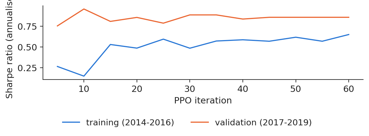
The training Sharpe ratio rises with the iterations, while the validation ratio is noisy; buy-and-hold had a Sharpe ratio of 0.95 on the validation years, and the selected iteration is on average the 48th.

Chart: Training and validation Sharpe ratios during PPO training

Annualised Sharpe ratio of the greedy policy on the last three training years and on the validation years, during training; band = range over five seeds.

Source: Yahoo Finance, daily quotes. Data: training windows from 17 Oct 2005 to 30 Dec 2016; band = range over 5 seeds.

Test period: the PPO agent against two simple rules

Slide 33 in the PDF

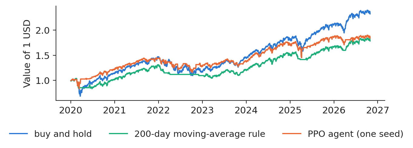
On the test period the Sharpe ratio is 0.61 for buy-and-hold, 0.68 for the moving-average rule and 0.83 for PPO, averaged over seeds that range from 0.72 to 0.95.

Chart: Test period: the PPO agent against two simple rules

Value of 1 USD invested on 2 January 2020 in each strategy, after a 5 basis-point cost per change of position; band = range over five PPO seeds.

Source: Yahoo Finance, daily quotes. Data: 2 Jan 2020 to 29 Oct 2026 (test), S&P 500, 5 bp cost per trade.

Trading results on the test period

Slide 34 in the PDF
StrategyReturn %/yrVolatility %/yrSharpeMax. drawdown %Invested %Trades
Buy and hold13.220.20.61−33.91001
200-day moving average8.912.40.68−20.57941
PPO (mean of 5 seeds)15.117.00.83−23.282147

PPO has the higher Sharpe ratio in all five seeds, but the stationary block bootstrap (Politis & Romano, 1994) of the Sharpe difference between the seed-averaged PPO strategy and buy-and-hold, +0.26, gives a 95 % interval of [−0.08; 0.56]. The interval contains zero: the data do not establish that the agent adds value.

In practice: an interval that contains zero means no evidence that the agent adds value, whatever the backtest chart suggests.

Periods in which the agent is out of the market

Slide 35 in the PDF

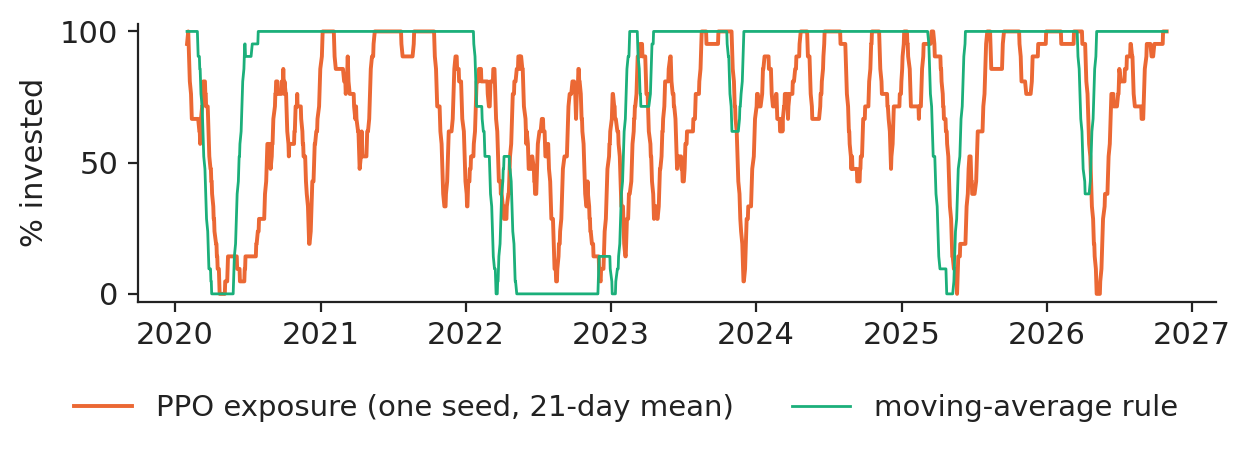
Reading the positions tells what the agent actually does. PPO was invested on 82 % of the test days. Between 20 February and 30 April 2020 it was invested 42 % of the time, against 14 % for the moving-average rule; in 2022 it was invested 63 % of the time, against 15 %. The agent cuts exposure in stress, but less than the trend rule.

Chart: Periods in which the agent is out of the market

Share of capital invested by the PPO agent (mean over seeds, 21-day mean) and by the moving-average rule.

Source: Yahoo Finance, daily quotes. Data: 2 Jan 2020 to 29 Oct 2026 (test).

In practice: read the policy, not only its profit: an agent that is simply always long is buy-and-hold with extra model risk.

Limitations of backtests for RL trading agents

Slide 36 in the PDF

Daily equity returns are close to unpredictable, so the agent mostly learns the noise of its training windows. Markets are non-stationary: the training years contain 2008, the test years a pandemic crash, an inflation shock and a long rally. Five seeds already give a range of Sharpe ratios, and reporting the best is backtest overfitting. A price-taking simulator ignores market impact, and costs must be in the reward. RL helps more in problems with a real state and a known reward: order execution, market making, hedging and storage (Hambly, Xu & Yang, 2023).

In practice: ask for the seed distribution, the cost assumption and a bootstrap interval before trusting any RL trading result.

Deep hedging: a policy that minimises tail risk

Deep hedging (Buehler et al., 2019) trains a neural hedging policy on the risk measure the desk reports.

Hedging a short call: the profit and loss of the desk

Slide 38 in the PDF

The desk sells a one-month at-the-money (ATM) call on the S&P 500 and trades the index every day:

\[\mathrm{PL}(\delta)=C_0+\sum_{k=0}^{20}\delta_k(S_{k+1}-S_k)-(S_{21}-K)^{+}-c\sum_{k=0}^{21}S_k|\delta_k-\delta_{k-1}|\]
(10.11)

where \(S_k\) is the index on day \(k\) of a real 21-day path (scaled so that \(S_0=K=1\)), \(C_0\) the Black-Scholes premium with the VIX of day 0 as volatility and a zero rate, \(\delta_k\) the units held over \((k,k+1]\) and \(c=10\) basis points. There is one path per start day: 3,021 for training (2005–2016), 754 for validation and 1,696 for the test (from 2020). On the test paths the mean premium is 2.38 % of the index and the mean payoff 2.53 %, with a mean VIX of 20.7. The paths are real, not simulated, so they keep the jumps and volatility clusters of 2008, 2020 and 2022.

In practice: the premium barely covers the mean payoff; the risk desk manages the tail.

Black-Scholes delta and the deep-hedging objective

Slide 39 in the PDF

The benchmark holds the Black-Scholes delta \(\delta_k=\Phi(d_1)\), \(d_1=[\ln(S_k/K)+\tfrac12\sigma_k^2\tau_k]/(\sigma_k\sqrt{\tau_k})\), with \(\sigma_k\) the VIX of day \(k\) and \(\tau_k=(21-k)/252\). The network \(\delta_\theta(\ln S_k,\tau_k,\sigma_k,\delta_{k-1})\in[0,1]\) instead minimises the expected shortfall of the loss, in the form of Rockafellar & Uryasev (2000):

\[\min_{\theta,w}\ w+\frac{1}{1-\alpha}\mathbb E\big[(-\mathrm{PL}(\delta_\theta)-w)^{+}\big]=\min_\theta\mathrm{ES}_\alpha\big(-\mathrm{PL}(\delta_\theta)\big),\qquad \alpha=0.95\]
(10.12)

At the optimum \(w\) is the value at risk (VaR). The profit and loss is differentiable in \(\theta\), so the gradient flows back through all 21 days; the previous hedge as an input lets the network learn a no-trade band when costs are high.

In practice: the objective is the risk measure the desk reports.

Hedging profit and loss on the test paths

Slide 40 in the PDF

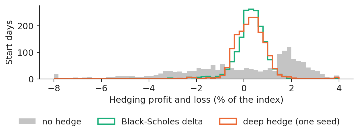
Hedging removes most of the left tail. The standard deviation of the profit and loss is 2.60 % of the index without hedge, 0.74 % with the delta hedge and 0.69 % with the deep hedge.

Chart: Hedging profit and loss on the test paths

Distribution of the hedging profit and loss on the test paths, in % of the initial index level: no hedge, Black-Scholes delta, deep hedge (first seed).

Source: Yahoo Finance, daily quotes. Data: 21-day paths starting 2 Jan 2020 to 1 Oct 2026 (test); S&P 500 and VIX; 10 bp cost.

Hedging results on the test paths, 10 bp cost

Slide 41 in the PDF
StrategyMean PL (%)Std. dev. (%)ES95 of loss (%)Turnover
No hedge−0.152.606.820
Black-Scholes delta (VIX)0.240.741.941.71
Deep hedge (mean of 5 seeds)0.270.691.151.32

The ES of the deep hedge ranges from 1.10 to 1.24 across seeds and is below the delta hedge in all five seeds, while the deep hedge also trades less.

In practice: judge a hedge by the tail of the loss and by its turnover, not by its mean profit.

The learned hedge ratio: flatter and adjusted for costs

Slide 42 in the PDF

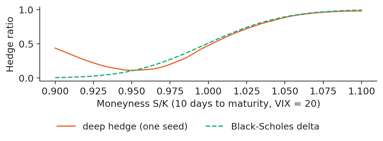
Ten days before maturity, with the VIX at 20, the learned hedge ratio is flatter than the delta around the strike: 0.46 at the money against 0.51 for Black-Scholes. The network has learned to trade less where trading is expensive and the payoff uncertain.

Chart: The learned hedge ratio: flatter and adjusted for costs

Hedge ratio of the deep hedge (mean and range of five seeds) and the Black-Scholes delta as a function of moneyness.

Source: Yahoo Finance, daily quotes. Data: policy trained on 21-day paths starting 2005-2016.

Transaction costs and the advantage of the learned hedge

Slide 43 in the PDF

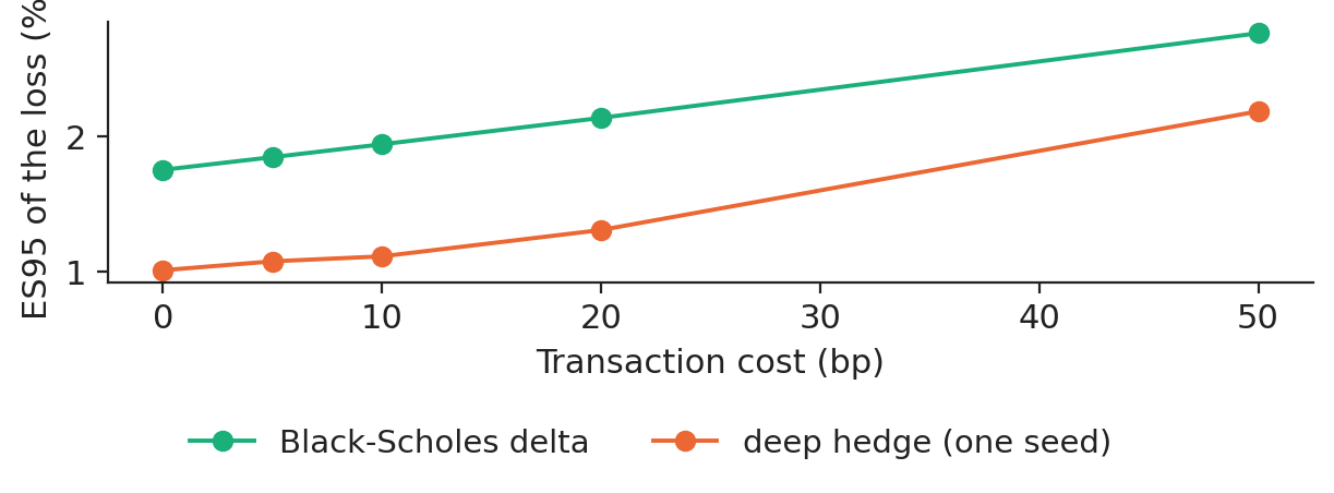
One network was trained for each cost level from 0 to 50 basis points. Without costs the ES95 is 1.75 % for the delta and 0.90 % for the deep hedge; at 50 basis points, 2.76 % and 2.34 %. The learned hedge also adapts to the real, fat-tailed paths, not only to costs.

Chart: Transaction costs and the advantage of the learned hedge

ES95 of the hedging loss on the test paths as a function of the transaction cost: Black-Scholes delta and deep hedge (mean of three seeds per cost level).

Source: Yahoo Finance, daily quotes. Data: test paths starting 2 Jan 2020 to 1 Oct 2026.

In practice: the value of a learned hedge grows with frictions: illiquid underlyings, wide spreads, energy and commodity hedges.

Reinforcement learning in production: model risk

Slide 44 in the PDF

The agent optimises exactly the reward it is given: omit costs, risk or constraints and it will exploit the gap. A historical replay ignores the agent's own price impact and future regimes. Offline evaluation needs one test period used once, several seeds and a test against the rule in use. In production, action masks, position limits, a kill switch and human sign-off limit the damage; a table or a hedge-ratio curve can be audited, and Lecture 11 explains neural policies; and the live capture ratio and turnover should be compared with the backtest every month.

In practice: treat an RL policy like any model of the bank: documented, validated independently, monitored, with a fallback rule.

Section summary

On real data the three problems give three verdicts: for the battery, the simple rule wins; for trading, PPO's higher Sharpe ratio is not significant; for hedging, the learned policy wins in every seed. Lecture 11 opens the black box and explains what a neural network has learned.

Videos: the intuition behind the mathematics (in English)

Abbreviations

A2Cadvantage actor-critic
AIartificial intelligence
ASEBucharest University of Economic Studies
ATMat the money (strike = current price)
BGBulgaria (bidding zone)
CETCentral European Time
CPUcentral processing unit
DE-LUGermany-Luxembourg bidding zone
DMDiebold-Mariano test
DPdynamic programming
DQNdeep Q-network
ENTSO-EEuropean Network of Transmission System Operators for Electricity
ESexpected shortfall
EUEuropean Union
EUReuro
GAEgeneralised advantage estimation
HUHungary (bidding zone)
IPEInstitute for Economic Forecasting, Romanian Academy
ISEFraunhofer Institute for Solar Energy Systems
KLKullback-Leibler divergence
MDPMarkov decision process
MLPmultilayer perceptron
MWmegawatt
MWhmegawatt-hour
PPOproximal policy optimisation
ReLUrectified linear unit
RLreinforcement learning
RORomania (bidding zone)
SSRNSocial Science Research Network
TDtemporal difference
TRPOtrust region policy optimisation
USDUS dollar
VaRvalue at risk
VIXCboe Volatility Index (30-day implied volatility of the S&P 500)

References

  • Andrei, A.-V., Cepoi, C. O., Dumitrescu, B. A., Lessmann, S., Chiriac (Luchian), A.-C., Pele, D. T. & Petukhina, A. (2026). Joint probabilistic forecasting for battery arbitrage in day-ahead power markets. SSRN Working Paper 6872381. doi:10.2139/ssrn.6872381
  • Anagnoste, S., Andrei, A.-V., Bolovăneanu, V., Cepoi, C.-O., Clodnitchi, R., Cramer, A.-A., Grecu, R.-A., Lessmann, S., Pele, D. T., Petukhina, A. & Strat, V. A. (2025). The role of AI in (re)shaping energy finance: A systematic literature review. Energy Strategy Reviews, 61, 101833. doi:10.1016/j.esr.2025.101833
  • Andrei, A.-V., Velev, G., Toma, F.-M., Pele, D. T. & Lessmann, S. (2024). Energy price modelling: A comparative evaluation of four generations of forecasting methods. arXiv:2411.03372
  • Bellman, R. (1957). Dynamic Programming. Princeton University Press.
  • Buehler, H., Gonon, L., Teichmann, J. & Wood, B. (2019). Deep hedging. Quantitative Finance, 19(8), 1271–1291. doi:10.1080/14697688.2019.1571683
  • Diebold, F. X. & Mariano, R. S. (1995). Comparing predictive accuracy. Journal of Business & Economic Statistics, 13(3), 253–263. doi:10.1080/07350015.1995.10524599
  • Hambly, B., Xu, R. & Yang, H. (2023). Recent advances in reinforcement learning in finance. Mathematical Finance, 33(3), 437–503. doi:10.1111/mafi.12382
  • Mnih, V. et al. (2015). Human-level control through deep reinforcement learning. Nature, 518, 529–533. doi:10.1038/nature14236
  • Moody, J. & Saffell, M. (2001). Learning to trade via direct reinforcement. IEEE Transactions on Neural Networks, 12(4), 875–889. doi:10.1109/72.935097
  • Politis, D. N. & Romano, J. P. (1994). The stationary bootstrap. Journal of the American Statistical Association, 89(428), 1303–1313. doi:10.1080/01621459.1994.10476870
  • Rockafellar, R. T. & Uryasev, S. (2000). Optimization of conditional value-at-risk. Journal of Risk, 2(3), 21–41. doi:10.21314/JOR.2000.038
  • Schulman, J., Moritz, P., Levine, S., Jordan, M. & Abbeel, P. (2016). High-dimensional continuous control using generalized advantage estimation. ICLR. arXiv:1506.02438
  • Schulman, J., Wolski, F., Dhariwal, P., Radford, A. & Klimov, O. (2017). Proximal policy optimization algorithms. arXiv:1707.06347
  • Sutton, R. S. & Barto, A. G. (2018). Reinforcement Learning: An Introduction, 2nd ed. MIT Press. incompleteideas.net/book
  • Sutton, R. S., McAllester, D., Singh, S. & Mansour, Y. (2000). Policy gradient methods for reinforcement learning with function approximation. Advances in Neural Information Processing Systems, 12, 1057–1063.
  • van Hasselt, H., Guez, A. & Silver, D. (2016). Deep reinforcement learning with double Q-learning. Proceedings of the AAAI Conference on Artificial Intelligence, 30(1). doi:10.1609/aaai.v30i1.10295
  • Watkins, C. J. C. H. & Dayan, P. (1992). Q-learning. Machine Learning, 8, 279–292. doi:10.1007/BF00992698
  • Williams, R. J. (1992). Simple statistical gradient-following algorithms for connectionist reinforcement learning. Machine Learning, 8, 229–256. doi:10.1007/BF00992696

Text written for the web version of the lecture; numbers, charts and sources come from the slides and their Quantlets.