Neural Networks and Deep Learning

Lecture 11: Explainable AI: SHAP, LIME, gradient methods and the stability of explanations

Lecture 11

Explainable AI: SHAP, LIME, gradient methods and the stability of explanations

Prof. dr. Daniel Traian PELE

Bucharest University of Economic Studies (ASE), Department of Statistics and Econometrics
Romanian Academy, Institute for Economic Forecasting (IPE)

A bank that rejects a loan applicant with a neural network must be able to say why. The European Union (EU) Artificial Intelligence (AI) Act classifies credit scoring of natural persons as high-risk, the General Data Protection Regulation (GDPR) protects people against decisions taken solely by machines, and model-risk supervisors ask for models that can be validated and monitored. This lecture shows how to open the black box with the methods of explainable artificial intelligence (XAI): Shapley additive explanations (SHAP), local interpretable model-agnostic explanations (LIME), gradient methods such as integrated gradients (IG), partial dependence and counterfactual explanations.

Every method is computed on real data. The credit case uses the home-equity loan data set (HMEQ): 5,960 loans, 19.9 % of them in default, scored by a multilayer perceptron (MLP), a logistic regression and extreme gradient boosting (XGBoost). The fraud case uses two days of credit-card transactions released by the Université Libre de Bruxelles (ULB): a network trained on the first day is explained on the second. The housing case uses the 1990 California census. The second half of the lecture asks a question that is often skipped: are the explanations faithful to the model, and do they stay the same when nothing important changes?

What you will be able to do

  • Explain why banks, insurers and regulators require explanations, and classify explanation methods.
  • Compute and read SHAP and LIME explanations with their full formulas, for one customer and for a portfolio.
  • Use saliency, integrated gradients and SmoothGrad, and check the completeness axiom on a real fraud model.
  • Test whether explanations agree, are faithful and stay stable across seeds, samples and time.
  • Write a counterfactual explanation that a rejected applicant can act on.

Lecture plan

  1. Reasons for explaining neural networksExplanations are required by law and by good risk management, but an explanation is itself a model of the model.
  2. Shapley values and SHAPShapley values come from cooperative game theory: they split a total payoff among players in the only way that satisfies four fairness axioms.
  3. LIME, counterfactuals and global effectsLIME explains a prediction by a simple model fitted around it; counterfactuals say what would have to change; partial dependence shows the average effect of one feature.
  4. Gradient methods for neural networksA network gives its gradients for free: one backward pass yields the sensitivity of the output to every input.
  5. Agreement, faithfulness and stability of explanationsThree tests should accompany every explanation: agreement between methods, faithfulness to the model and stability when nothing important changes.
  6. Explainability in model governance

Reasons for explaining neural networks

Explanations are required by law and by good risk management, but an explanation is itself a model of the model. This section sets out the rules, a taxonomy of methods and the credit case that runs through the lecture.

Regulators require explanations of automated decisions

Slide 6 in the PDF

Three texts frame the European practice. The AI Act (Regulation 2024/1689) lists creditworthiness assessment of natural persons among high-risk uses (Annex III), requires providers to make the system transparent to those who deploy it (article 13) and gives a person affected by a decision the right to an explanation of the role the system played (article 86). The GDPR, article 22 and recital 71, adds safeguards against decisions based solely on automated processing. The European Banking Authority (EBA) guidelines on loan origination and monitoring (2020) require that models used for credit decisions can be explained. Outside the EU, the Federal Reserve Supervisory Guidance on Model Risk Management (SR 11-7) asks for conceptual soundness, independent validation and ongoing monitoring of every model.

There are business reasons too: explanations reveal leakage (a feature that should not be there), help credit officers trust a score and let the bank tell a customer why the answer was no. The caveat runs through the whole lecture: an explanation that changes when nothing important has changed is a compliance risk, not a safeguard.

In practice: an explanation that changes when nothing important changed is a compliance risk, not a safeguard.

A taxonomy of explanation methods

Slide 7 in the PDF

Methods differ in scope and in what they need. Global methods describe the model over the whole population (coefficients, mean absolute SHAP values, partial dependence, permutation importance); local methods explain one decision (a SHAP waterfall, LIME, gradients, a counterfactual). Model-agnostic methods only call the model (Kernel SHAP, LIME, partial dependence); model-specific methods use its structure (TreeSHAP for trees, gradients for networks). Finally, post-hoc methods explain a model that is already trained, while interpretable models such as a scorecard are transparent by design. Rudin (2019) argues that in high-stakes decisions the second route should be tried first; we will see how much accuracy it costs on our data.

Credit case study: comparison of three scoring models

Slide 8 in the PDF

The network has two hidden layers of 64 and 32 rectified linear units (ReLU):

\[\mathbf h_1=\mathrm{ReLU}(\mathbf W_1\mathbf x+\mathbf b_1),\quad \mathbf h_2=\mathrm{ReLU}(\mathbf W_2\mathbf h_1+\mathbf b_2),\quad f(\mathbf x)=\mathbf w_3^{\top}\mathbf h_2+b_3,\quad \mathrm{PD}(\mathbf x)=\sigma(f(\mathbf x))\]
(11.1)

where \(\mathbf x\) holds 18 standardised features (ten numeric variables imputed with the training median, a flag for a missing debt-to-income ratio, DEBTINC, the loan reason and the job), \(f\) is the log-odds of default and PD the probability of default. The loans are split 60/20/20 with stratification; the scalers and medians are fitted on the training part only.

Model (test)AUCPR-AUCBrier
Logistic regression0.9090.7850.080
MLP, mean of 10 seeds0.9350.8420.068
XGBoost, mean of 10 seeds0.9590.8890.058

AUC is the area under the receiver operating characteristic (ROC) curve and PR-AUC the area under the precision-recall curve; a random score has a PR-AUC equal to the default rate, 0.200. The network is clearly better than the logistic scorecard, and the boosted trees are better still. For the logistic model the coefficients are the explanation; for the network the explanation has to be computed.

In practice: the logistic coefficients are the explanation; for the MLP the explanation must be computed.

Shapley values and SHAP

Shapley values come from cooperative game theory: they split a total payoff among players in the only way that satisfies four fairness axioms. SHAP applies them to the features of one prediction.

Shapley values: a fair split of the prediction among features

Slide 10 in the PDF

For \(d\) features and a value function \(v(S)\) that says what the model predicts when only the features in \(S\) are known, the Shapley value of feature \(j\) is its marginal contribution averaged over all orders in which the features could be added:

\[\phi_j=\sum_{S\subseteq\{1,\dots,d\}\setminus\{j\}}\frac{|S|!\,(d-|S|-1)!}{d!}\big[v(S\cup\{j\})-v(S)\big]\]
(11.2)

The weights are the share of orderings in which \(j\) arrives right after the members of \(S\). Shapley (1953) proved that this is the only split with four properties: efficiency (the contributions add up to \(v\) of all features minus \(v\) of none), symmetry (two features that contribute equally get the same share), dummy (a feature that never changes \(v\) gets zero) and additivity. The price is computational: with 18 features there are \(2^{18}\) coalitions for every applicant.

In practice: efficiency is what a credit officer needs: the parts add up exactly to the score.

SHAP: the value of a coalition of features

Slide 11 in the PDF

SHAP (Lundberg & Lee, 2017) defines the value of a coalition as the expected model output when the missing features are drawn from a background sample \(\mathcal B\) of 100 training applicants:

\[v(S)=\mathbb E_{\mathbf x_{\bar S}\sim\mathcal B}\big[f(\mathbf x_S,\mathbf x_{\bar S})\big],\qquad f(\mathbf x)=\phi_0+\sum_{j=1}^{d}\phi_j(\mathbf x),\quad \phi_0=\mathbb E_{\mathcal B}[f]\]
(11.3)

We explain the log-odds, where effects add. On 400 test applicants the largest additivity error is \(2.9\cdot10^{-6}\), rounding error only. For a linear model the formula has a closed form, \(\phi_j=\beta_j(x_j-\mathbb E x_j)\) (linear SHAP). The replacement of missing features is interventional, that is, independent of the known ones; when features are correlated this can create applicants that do not exist, a limitation to state in the model documentation.

In practice: the background sample defines the "average applicant"; document it like any model input.

Kernel SHAP and TreeSHAP: how SHAP is computed

Slide 12 in the PDF

Kernel SHAP fits a weighted linear regression of the coalition values on coalition indicators \(\mathbf z\in\{0,1\}^d\), with the Shapley kernel

\[\pi(\mathbf z)=\frac{d-1}{\binom{d}{|\mathbf z|}\,|\mathbf z|\,(d-|\mathbf z|)}\]
(11.4)

and the weighted least-squares solution equals the Shapley values (the proof is in Appendix A of the slides). We sample 600 coalitions per applicant; the 400 applicants take 16 seconds. For tree ensembles TreeSHAP computes the exact values in polynomial time (Lundberg et al., 2020), which is how we explain XGBoost. Kernel SHAP has sampling noise, so its seed and sample size belong in the documentation.

Global importance: the missing debt-to-income ratio dominates

Slide 13 in the PDF

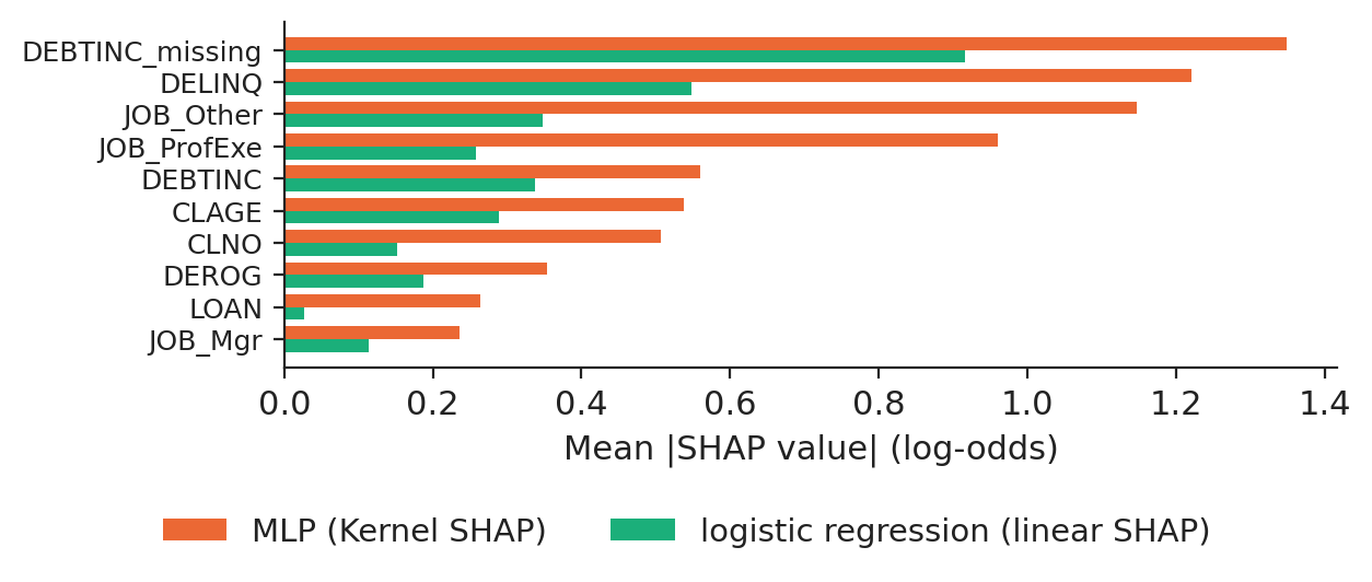
The mean absolute SHAP value of each feature ranks the drivers of the portfolio. All three models put the flag DEBTINC_missing first; for the network it is followed by DELINQ, the number of delinquent credit lines, and by the job category "Other". The Spearman correlation of the importances is 0.55 between the MLP and XGBoost and 0.79 between the MLP and the logistic regression.

The reason is in the data: the debt-to-income ratio is missing for 21.3 % of the loans, and the default rate is 62.0 % when it is missing against 8.6 % when it is reported. The network has learned that an incomplete file is a strong signal of risk.

Chart: Global importance: the missing debt-to-income ratio dominates

Mean absolute SHAP value of the ten most important features for the MLP (Kernel SHAP), XGBoost (TreeSHAP) and the logistic regression (linear SHAP), on 400 test applicants.

Source: Baesens, Roesch and Scheule (2016), HMEQ data. Data: 400 test applicants, 100 background applicants.

In practice: an explanation can reveal that a model scores the paperwork rather than the borrower; decide whether that is acceptable.

The beeswarm: direction and spread of every effect

Slide 14 in the PDF

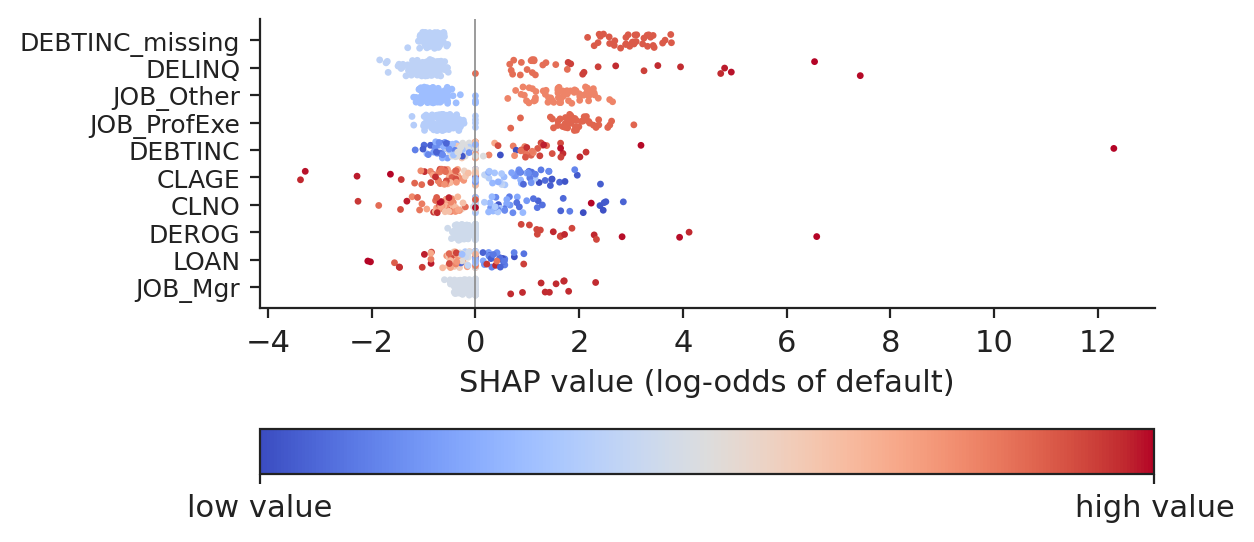
The beeswarm shows each applicant as a dot, placed at its SHAP value and coloured by the rank of the feature value. It adds what the bar chart hides: the direction of the effect and its spread. High values of DELINQ and of DEROG, the number of major derogatory reports, push the risk up, as credit theory expects; a reported debt-to-income ratio lowers it for most applicants.

Chart: The beeswarm: direction and spread of every effect

SHAP values of the ten most important features for 400 test applicants; colour from blue (low value) to red (high value).

Source: Baesens, Roesch and Scheule (2016), HMEQ data. Data: 400 test applicants; colour = rank of the feature value.

Local explanation of a rejected applicant: SHAP waterfall

Slide 15 in the PDF

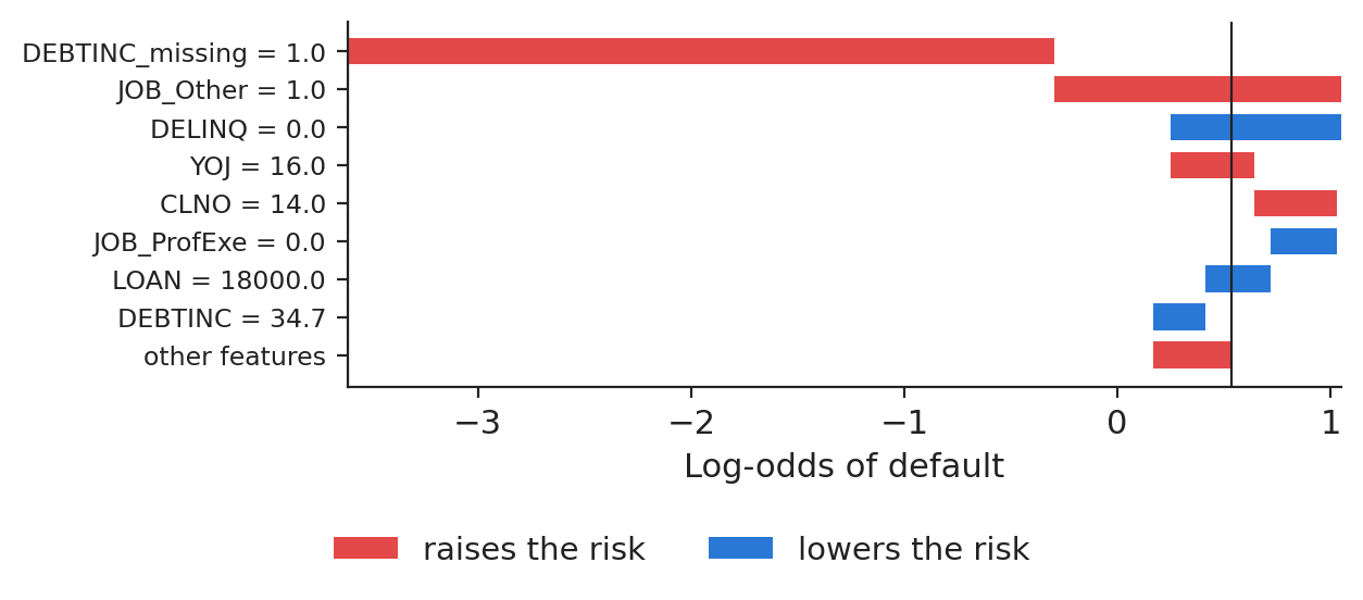
For one test applicant (row 2411 of the data) the network gives a PD of 65.6 %, log-odds 0.648. The waterfall starts from the average log-odds \(\phi_0=-3.613\) and adds the contributions one by one until it reaches the applicant's score: \(-3.613+4.261=0.648\). The largest pushes are DEBTINC_missing (\(+3.13\)), the job category "Other" (\(+1.74\)) and DELINQ (\(-0.71\), this applicant has no delinquent lines).

Chart: Local explanation of a rejected applicant: SHAP waterfall

Contributions of the eight largest features (values in original units) and of the remaining ten, from the average log-odds to the applicant's log-odds.

Source: Baesens, Roesch and Scheule (2016), HMEQ data. Data: test applicant (row 2411); values in original units.

In practice: the adverse-action notice lists the top reasons in this order, in words the customer understands.

Dependence plot: the network learned the missing-value signal

Slide 16 in the PDF

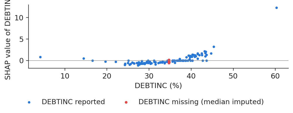
Plotting the SHAP value of DEBTINC against DEBTINC shows a second effect of imputation. Applicants whose ratio is missing all sit at the training median and their SHAP value for DEBTINC is small: the risk of these files is carried by the missing flag, whose mean SHAP value is \(+3.13\). Without the flag, the network would have to guess the risk from the imputed value, and the explanation would blame a debt-to-income ratio the applicant never reported.

Chart: Dependence plot: the network learned the missing-value signal

SHAP value of DEBTINC against the reported ratio (blue) and for files with a missing ratio, imputed at the median (red).

Source: Baesens, Roesch and Scheule (2016), HMEQ data. Data: 400 test applicants, MLP.

In practice: imputation choices change explanations; keep a missing-value flag so that the reason can be named.

LIME, counterfactuals and global effects

LIME explains a prediction by a simple model fitted around it; counterfactuals say what would have to change; partial dependence shows the average effect of one feature.

LIME: a simple model that is faithful near one point

Slide 18 in the PDF

LIME (Ribeiro, Singh & Guestrin, 2016) perturbs the applicant, weights the perturbations by their distance and fits a linear model to the network's answers:

\[\xi(\mathbf x)=\arg\min_{g\in\mathcal G}\sum_{\mathbf z}\pi_{\mathbf x}(\mathbf z)\big[f(\mathbf z)-g(\mathbf z)\big]^2+\Omega(g),\qquad \pi_{\mathbf x}(\mathbf z)=\exp\!\Big(-\frac{\|\mathbf z-\mathbf x\|^2}{\sigma^2}\Big)\]
(11.5)

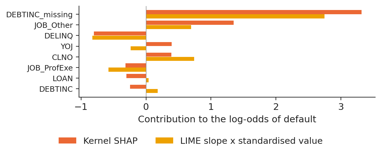
where \(\mathcal G\) is the set of linear models, \(\Omega\) a complexity penalty and \(\sigma\) the kernel width, \(0.75\sqrt d=3.18\) by default. LIME gives a local slope, not a split of the prediction, so its coefficients do not add up to \(f(\mathbf x)\). For our applicant LIME's top feature is DELINQ, while SHAP's is DEBTINC_missing: a binary flag is far from a linear function, and the two methods answer different questions.

In practice: LIME answers "what moves the score near this customer?", SHAP answers "why is this customer far from average?".

LIME and SHAP for the same applicant

Slide 19 in the PDF

To compare the two on one scale we multiply each LIME slope by the standardised value of the feature, which gives a contribution relative to the average applicant. The Spearman correlation of the absolute contributions is 0.80: the two methods agree on most of the ranking but not on the top feature.

Chart: LIME and SHAP for the same applicant

Kernel SHAP contribution and LIME slope × standardised value for the eight largest SHAP features of the same applicant (LIME with 5,000 samples).

Source: Baesens, Roesch and Scheule (2016), HMEQ data. Data: test applicant (row 2411); LIME with 5,000 samples.

Sensitivity of LIME to its settings

Slide 20 in the PDF

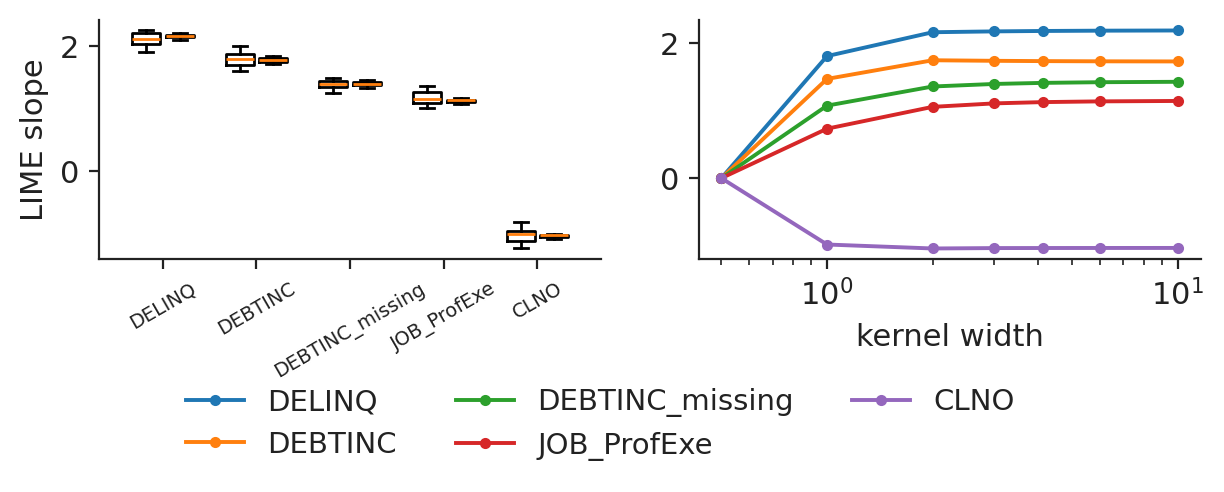
We repeated LIME 30 times with different seeds. With 500 samples the top feature was the same in 73 % of the runs and the Jaccard overlap of the top-5 sets was 0.72; with 5,000 samples, in 100 % of the runs, overlap 1.00. The coefficient of variation of the five largest slopes falls from 10 % to 2 %. The kernel width matters as much: the slope of the top feature moves between \(0.001\) and \(2.042\) as \(\sigma\) goes from 0.5 to 10.

Chart: Sensitivity of LIME to its settings

Left: LIME slopes of five features over 30 runs with 500 and with 5,000 samples. Right: the same slopes as a function of the kernel width (dashed line: default).

Source: Baesens, Roesch and Scheule (2016), HMEQ data. Data: test applicant (row 2411); right panel: same five features, 5,000 samples.

In practice: fix and report the seed, sample size and kernel width of every LIME explanation that reaches a customer or an auditor.

Counterfactual explanations: minimal changes that reverse the decision

Slide 21 in the PDF

A counterfactual (Wachter, Mittelstadt & Russell, 2017) looks for the closest applicant whom the model would accept, changing only features the applicant can act on:

\[\mathbf x'=\arg\min_{\mathbf x'}\ \lambda\,\big(f(\mathbf x')-t\big)_+^{2}+\sum_{j\in\mathcal A}\frac{|x'_j-x_j|}{\mathrm{MAD}_j}\]
(11.6)

where \(t=-0.5\) is a target log-odds below the 0.5 PD threshold, \(\mathcal A\) the actionable features (LOAN, DEBTINC, NINQ, DELINQ, DEROG, CLNO, MORTDUE) and the median absolute deviation (MAD) puts all distances on a comparable scale. Raw values are kept non-negative and counts are rounded. For our applicant the optimisation lowers the outstanding mortgage from 69,115 to 57,456.5, the debt-to-income ratio from 34.7 to 33.4 and changes the loan amount from 14,500 to 15,700; the PD falls from 65.6 % to 39.2 %.

A second, simpler counterfactual is more useful: if the applicant reports the debt-to-income ratio (at the median value, 34.7), the PD becomes 5.1 %. The explanation points to the missing document, not to the applicant's finances.

In practice: "bring the missing income document" is a better answer to the customer than any list of SHAP values.

Global effects: partial dependence and ICE

Slide 22 in the PDF

The partial dependence of feature \(j\) averages the prediction over the data while \(j\) is set to a grid value; individual conditional expectation (ICE) keeps one curve per observation (Friedman, 2001; Goldstein et al., 2015):

\[\mathrm{PD}_j(z)=\frac1n\sum_{i=1}^{n}f(z,\mathbf x_{i,-j}),\qquad \mathrm{ICE}_{i,j}(z)=f(z,\mathbf x_{i,-j})\]
(11.7)

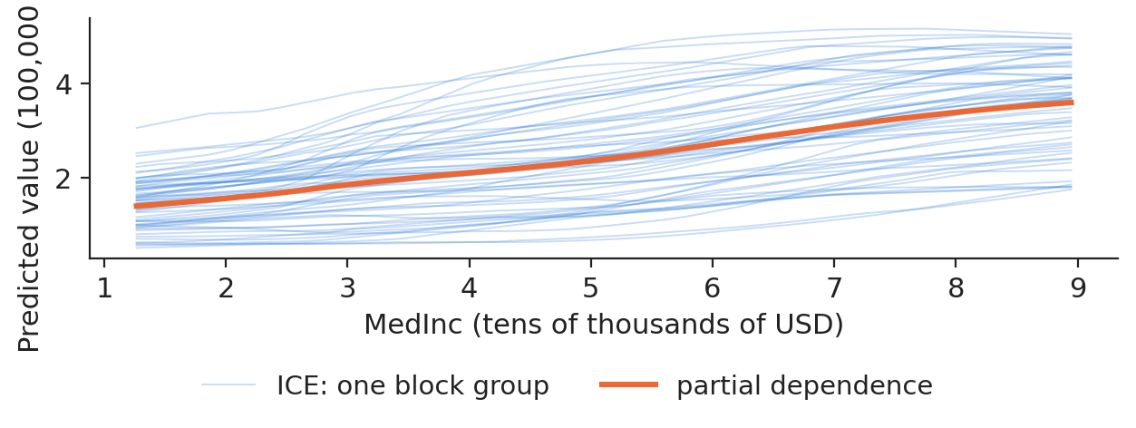
On California housing the MLP explains house values far better than a linear regression (test \(R^2\) 0.819 against 0.620). The partial dependence on median income rises from 1.40 to 3.60 (hundreds of thousands of US dollars, USD) over the income grid, and flattens at the top, where the data source caps the value at 5. The ICE curves fan out: at the top of the grid their standard deviation is 0.95, so the same income effect is not shared by all neighbourhoods. A partial dependence plot assumes that income can change while everything else stays fixed; with correlated features (income and rooms per household, correlation 0.33) it averages over combinations that may be rare.

Chart: Global effects: partial dependence and ICE

Partial dependence (orange, mean over 1,000 test block groups) and ICE curves (60 block groups) of the predicted house value on median income.

Source: StatLib, California housing, 1990 census (Pace and Barry, 1997). Data: MLP; 60 test block groups (ICE), 1,000 for the PDP.

Gradient methods for neural networks

A network gives its gradients for free: one backward pass yields the sensitivity of the output to every input. This section explains a fraud model with gradients.

Fraud case study: a network trained on day 1 and explained on day 2

Slide 24 in the PDF

The credit-card data cover two days of September 2013. The variables V1–V28 are principal component analysis (PCA) components released by the data owner, plus the transaction amount; frauds are 0.15 % of the transactions of day 2 once the sampling weights restore the full data. We train an MLP on day 1, with early stopping on the weighted validation PR-AUC, and test it on day 2: PR-AUC 0.815 against 0.742 for the logistic regression.

The simplest explanations are the saliency \(|\partial f/\partial x_j|\) (Simonyan, Vedaldi & Zisserman, 2014) and the gradient × input \((x_j-x'_j)\,\partial f/\partial x_j\), where \(\mathbf x'\) is a baseline, here the mean legitimate transaction of day 1. Both suffer from saturation: in a flat part of \(f\) the gradient is close to zero even for a decisive feature.

In practice: a fraud analyst gets a ranked list of the inputs that drove the alert, in milliseconds per transaction.

Integrated gradients and the completeness of attributions

Slide 25 in the PDF

Integrated gradients (Sundararajan, Taly & Yan, 2017) integrate the gradient along the straight path from the baseline to the input:

\[\mathrm{IG}_j(\mathbf x)=(x_j-x'_j)\int_0^1\frac{\partial f\big(\mathbf x'+\alpha(\mathbf x-\mathbf x')\big)}{\partial x_j}\,d\alpha\]
(11.8)

By the fundamental theorem of calculus for paths the attributions add up to \(f(\mathbf x)-f(\mathbf x')\) (completeness). IG also satisfies sensitivity and implementation invariance, and it is the Aumann–Shapley value of the continuous game along the path. In practice the integral is a Riemann sum with \(m\) steps. The baseline defines the question: with the mean legitimate transaction we ask "why is this not a normal payment?".

In practice: write the baseline into the model documentation: a different baseline is a different question.

Completeness holds once the integral is computed accurately

Slide 26 in the PDF

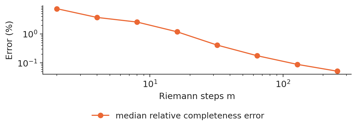
On the 211 frauds of day 2 the median relative completeness error is 3.7 % with 4 steps and 0.18 % with 64 steps; it falls roughly as \(1/m^2\), the rate of the midpoint rule.

Chart: Completeness holds once the integral is computed accurately

Median relative completeness error of integrated gradients against the number of Riemann steps (log scales).

Source: ULB Machine Learning Group and Worldline, credit-card transactions (OpenML 1597). Data: 211 frauds of day 2; baseline = mean legitimate transaction of day 1.

SmoothGrad and concept-level explanations

Slide 27 in the PDF

SmoothGrad (Smilkov et al., 2017) averages gradients over noisy copies of the input, which removes the jitter of a ReLU network. Testing with concept activation vectors (TCAV) (Kim et al., 2018) asks a different question: does a human concept, learned as a direction \(\mathbf v_C\) in a hidden layer, move the output? Concepts must be labelled, which is not possible with anonymised PCA components; plan them when the data are collected.

Four explanation methods for one fraudulent transaction

Slide 28 in the PDF

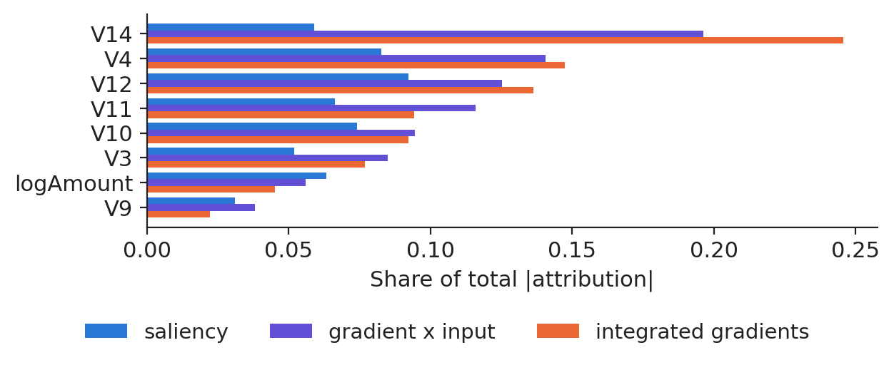
For the median-score fraud of day 2 (fraud score 99.9 %), Kernel SHAP and integrated gradients both name V14 as the main feature, while saliency names V12: saliency measures how sensitive the score is, not how far the transaction is from normal.

Chart: Four explanation methods for one fraudulent transaction

Signed attributions of saliency, gradient × input, integrated gradients and Kernel SHAP for one fraud, as shares of the total absolute attribution.

Source: ULB Machine Learning Group and Worldline, credit-card transactions (OpenML 1597). Data: one fraud of day 2 (median fraud score).

Agreement, faithfulness and stability of explanations

Three tests should accompany every explanation: agreement between methods, faithfulness to the model and stability when nothing important changes.

Agreement between explanation methods

Slide 30 in the PDF

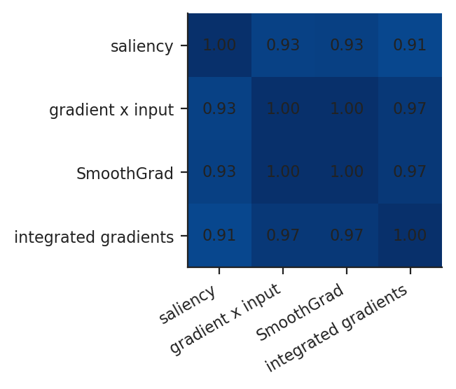
On the same 211 frauds we compare the global importances of seven methods. The Spearman correlation is 0.85 between IG and SHAP, 0.83 between saliency and SHAP, 0.82 between LIME and SHAP, and only 0.58 between permutation importance and SHAP; all methods put V12 first. The disagreement is informative: permutation importance (Breiman, 2001) measures how much the model needs a feature to stay accurate, attributions measure how much it uses the feature for the frauds.

Chart: Agreement between explanation methods

Spearman correlation of the global importances (mean absolute attribution) of seven explanation methods.

Source: ULB Machine Learning Group and Worldline, credit-card transactions (OpenML 1597). Data: Spearman correlation of global importances; 211 frauds of day 2.

In practice: disagreement is information: permutation importance measures what the model needs, attributions what it uses.

Faithfulness of explanations: deletion test

Slide 31 in the PDF

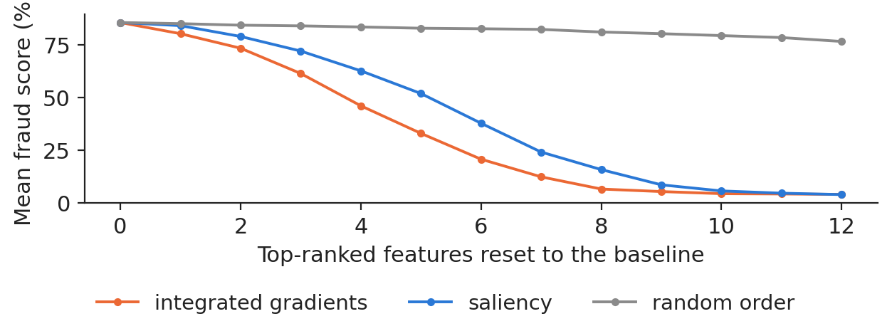
A faithful explanation names the features whose removal changes the prediction. We reset the top-\(k\) features of each fraud to the baseline and follow the mean fraud score; the area over the perturbation curve (AOPC) summarises the fall (Samek et al., 2017). In points of fraud score: IG 56.2, SHAP 58.4, LIME 56.1, saliency 48.0, random order 3.9. SHAP, IG and LIME are equally faithful here, saliency less so, and every method is far better than chance.

Chart: Faithfulness of explanations: deletion test

Mean fraud score of the day-2 frauds after resetting the \(k\) top-ranked features to the baseline, for four methods and a random order.

Source: ULB Machine Learning Group and Worldline, credit-card transactions (OpenML 1597). Data: 211 frauds of day 2.

Local robustness of explanations to small input changes

Slide 32 in the PDF

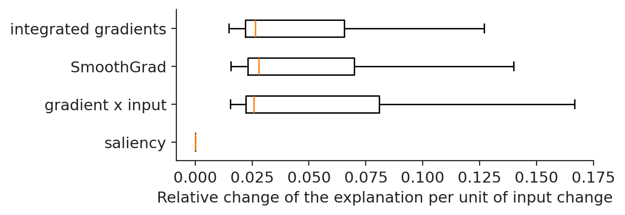
We add Gaussian noise with a standard deviation of 0.05 to 60 frauds, ten times, and measure the relative change of the attribution per unit of input change (Alvarez-Melis & Jaakkola, 2018). The medians are 0.000 for saliency, 0.028 for gradient × input, 0.030 for IG and 0.036 for SmoothGrad. Saliency does not move because inside one linear region of a ReLU network the gradient is constant: robustness to small noise comes with abrupt jumps between regions.

Chart: Local robustness of explanations to small input changes

Relative change of the explanation per unit of input change for four gradient methods (60 frauds × 10 perturbations).

Source: ULB Machine Learning Group and Worldline, credit-card transactions (OpenML 1597). Data: 60 frauds of day 2 x 10 perturbations (sigma = 0.05 standard deviations).

The Rashomon effect: equally accurate models with different explanations

Slide 33 in the PDF

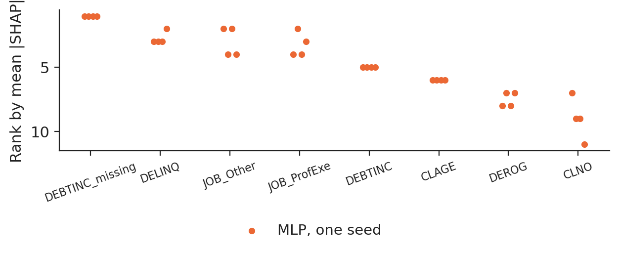
We retrained the credit models with ten seeds. The test AUC of the network stays between 0.929 and 0.941, but the order of the features moves: the mean pairwise Kendall \(\tau\) of the global importances is 0.83 for the MLP and 0.97 for XGBoost. For a single applicant the top feature is the same in 78 % of the seed pairs for the network and 83 % for XGBoost. Many models fit the data equally well, and they do not all tell the same story.

Chart: The Rashomon effect: equally accurate models with different explanations

Rank of each feature by mean absolute SHAP value for ten MLPs and ten XGBoost models that differ only in the training seed.

Source: Baesens, Roesch and Scheule (2016), HMEQ data. Data: 10 training seeds; 200 test applicants.

Explanations over time: day 1 against day 2

Slide 34 in the PDF

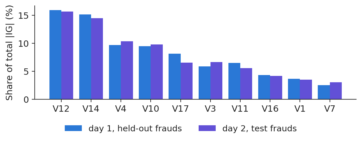
Distribution shift can change explanations even when the model is fixed. We compare the integrated gradients of the 70 held-out frauds of day 1 with those of the 211 frauds of day 2. The Spearman correlation of the importances is 0.98, the Jensen–Shannon (JS) divergence, built on the Kullback–Leibler (KL) divergence, is 0.003, and four of the top five features are shared: one day later, the explanation of this model is stable. Our group studies the same question over longer horizons and with graph features (see the research slide).

Chart: Explanations over time: day 1 against day 2

Share of the total absolute integrated gradients by feature, for held-out frauds of day 1 and for the frauds of day 2.

Source: ULB Machine Learning Group and Worldline, credit-card transactions (OpenML 1597). Data: model trained on day 1; integrated gradients.

In practice: monitor the distribution of attributions monthly, next to the score distribution; a drift in reasons can precede a drift in accuracy.

Stability scorecard of this lecture

Slide 35 in the PDF
Source of changeMeasureResult
Explainer randomness (LIME)same top feature over 30 runs73 % (500 samples), 100 % (5,000)
Training seedKendall \(\tau\) of global importancesMLP 0.83, XGBoost 0.97
Training seed, one applicantsame top featureMLP 78 %, XGBoost 83 %
MethodSpearman of importances0.52 to 1.00
Input noisemedian relative changeIG 0.030, SmoothGrad 0.036
Time (day 1 to day 2)Spearman, JS divergence0.98; 0.003
In practice: report every explanation with its stability: which seed, which sample, which period, and how much it moves.

Section summary

Explanations are estimates. SHAP adds up exactly, LIME depends on its settings, gradients are cheap and, with integrated gradients, complete; but every explanation moves with the seed, the sample and the period, and should be tested like a model.

Explainability in model governance

An explainability audit checklist

Slide 37 in the PDF

An audit of explanations starts from the purpose: who reads the explanation (customer, analyst, validator, regulator) and which decision it supports. The settings (background sample, baseline, seed, number of samples, kernel width) are versioned with the model. The checks are those of this lecture: additivity or completeness, faithfulness, stability across seeds and time, agreement of two methods. Fairness needs a look at protected attributes and their proxies, remembering that an explanation shows how a model uses a feature, not that the feature causes default. For customers, a few reasons and an actionable counterfactual are better than raw component names. And if an interpretable model is almost as accurate (here a logistic AUC of 0.909 against 0.935 for the network), it deserves consideration.

In practice: the validation report should contain the explanations and their stability tests, not only the accuracy.

Explore it visually

Free interactive tools and illustrated guides for this lecture; most run in the browser.

  • Neuronpedia: open-source platform for the interpretability of language models: sparse autoencoders split the activations of a layer into features, and each feature page lists the texts on which it fires most.
  • Neuronpedia: compare the two views: SHAP and LIME attribute one prediction to the inputs, while these features describe what the inside of the model represents.

Section summary

Lecture 12 moves to large language models, where explanations themselves become text, with new questions about faithfulness.

Videos: the intuition behind the mathematics (in English)

Abbreviations

AIartificial intelligence
AOPCarea over the perturbation curve
ASEBucharest University of Economic Studies
AUCarea under the ROC curve
EBAEuropean Banking Authority
EUEuropean Union
EUReuro
GDPRGeneral Data Protection Regulation
GNNgraph neural network
HMEQhome-equity loan data set
ICEindividual conditional expectation
IGintegrated gradients
IPEInstitute for Economic Forecasting, Romanian Academy
JSJensen-Shannon divergence
KLKullback-Leibler divergence
LIMElocal interpretable model-agnostic explanations
MADmedian absolute deviation
MLPmultilayer perceptron
PCAprincipal component analysis
PDprobability of default
PDPpartial dependence plot
PICBEProceedings of the International Conference on Business Excellence
PR-AUCarea under the precision-recall curve
ReLUrectified linear unit
ROCreceiver operating characteristic
SHAPShapley additive explanations
SRSupervisory Guidance on Model Risk Management (Federal Reserve SR 11-7)
TCAVtesting with concept activation vectors
ULBUniversité Libre de Bruxelles
USDUS dollar
XAIexplainable artificial intelligence
XGBoostextreme gradient boosting

References

  • Alvarez-Melis, D. & Jaakkola, T. S. (2018). On the robustness of interpretability methods. ICML Workshop on Human Interpretability in Machine Learning. arXiv:1806.08049
  • Andrei, A.-V. & Pele, D. T. (2025). Explainable AI for electricity price anomaly detection: A SHAP-driven approach in Romania's energy market. Preprints. doi:10.20944/preprints202508.0410.v1
  • Andrei, A.-V., Pele, D.-T. & Cramer, A.-A. (2026). Multi-horizon explainability in energy price forecasting: Disentangling market dynamics and renewable intermittency in Romania's liberalized electricity market. Proceedings of the International Conference on Business Excellence, 20(1), 104–117. doi:10.2478/picbe-2026-0014
  • Andrei, A.-V., Pele, D.-T., Cramer, A.-A., Amza, A. & Diaconu, D. (2026). Explainable AI-based early warning system for electricity price spikes: Evidence from the Romanian market. Proceedings of the International Conference on Business Excellence, 20(1), 4820–4836. doi:10.2478/picbe-2026-0352
  • Baesens, B., Roesch, D. & Scheule, H. (2016). Credit Risk Analytics: Measurement Techniques, Applications, and Examples in SAS. Wiley.
  • Breiman, L. (2001). Random forests. Machine Learning, 45, 5–32. doi:10.1023/A:1010933404324
  • Dal Pozzolo, A., Caelen, O., Johnson, R. A. & Bontempi, G. (2015). Calibrating probability with undersampling for unbalanced classification. IEEE SSCI, 159–166. doi:10.1109/SSCI.2015.33
  • Diaconu, D. & Pele, D. T. (2026). SHAP stability across random and forward-time validation in graph-augmented fraud detection. Submitted to Expert Systems with Applications. Code: github.com/QuantLet/GNN_XAI_Stability
  • Friedman, J. H. (2001). Greedy function approximation: A gradient boosting machine. Annals of Statistics, 29(5), 1189–1232. doi:10.1214/aos/1013203451
  • Goldstein, A., Kapelner, A., Bleich, J. & Pitkin, E. (2015). Peeking inside the black box: Visualizing statistical learning with plots of individual conditional expectation. Journal of Computational and Graphical Statistics, 24(1), 44–65. doi:10.1080/10618600.2014.907095
  • Kim, B. et al. (2018). Interpretability beyond feature attribution: Quantitative testing with concept activation vectors (TCAV). ICML. arXiv:1711.11279
  • Lundberg, S. M. & Lee, S.-I. (2017). A unified approach to interpreting model predictions. Advances in Neural Information Processing Systems, 30. arXiv:1705.07874
  • Lundberg, S. M. et al. (2020). From local explanations to global understanding with explainable AI for trees. Nature Machine Intelligence, 2, 56–67. doi:10.1038/s42256-019-0138-9
  • Ribeiro, M. T., Singh, S. & Guestrin, C. (2016). “Why should I trust you?” Explaining the predictions of any classifier. KDD, 1135–1144. doi:10.1145/2939672.2939778
  • Rudin, C. (2019). Stop explaining black box machine learning models for high stakes decisions and use interpretable models instead. Nature Machine Intelligence, 1, 206–215. doi:10.1038/s42256-019-0048-x
  • Samek, W., Binder, A., Montavon, G., Lapuschkin, S. & Müller, K.-R. (2017). Evaluating the visualization of what a deep neural network has learned. IEEE Transactions on Neural Networks and Learning Systems, 28(11), 2660–2673. doi:10.1109/TNNLS.2016.2599820
  • Shapley, L. S. (1953). A value for n-person games. In Contributions to the Theory of Games II, 307–317. Princeton University Press.
  • Simonyan, K., Vedaldi, A. & Zisserman, A. (2014). Deep inside convolutional networks: Visualising image classification models and saliency maps. ICLR Workshop. arXiv:1312.6034
  • Smilkov, D., Thorat, N., Kim, B., Viégas, F. & Wattenberg, M. (2017). SmoothGrad: Removing noise by adding noise. arXiv:1706.03825
  • Sundararajan, M., Taly, A. & Yan, Q. (2017). Axiomatic attribution for deep networks. ICML, 3319–3328. arXiv:1703.01365
  • Wachter, S., Mittelstadt, B. & Russell, C. (2017). Counterfactual explanations without opening the black box: Automated decisions and the GDPR. Harvard Journal of Law & Technology, 31(2), 841–887. doi:10.2139/ssrn.3063289
  • Regulation (EU) 2024/1689 (Artificial Intelligence Act), Official Journal of the European Union, L, 12 July 2024. data.europa.eu/eli/reg/2024/1689/oj
  • Board of Governors of the Federal Reserve System (2011). SR 11-7: Supervisory guidance on model risk management. federalreserve.gov

Text written for the web version of the lecture; numbers, charts and sources come from the slides and their Quantlets.