Neural Networks and Deep Learning

Lecture 14: Multimodal and vision-language models; synthesis of the course

Lecture 14

Multimodal and vision-language models; synthesis of the course

Prof. dr. Daniel Traian PELE

Bucharest University of Economic Studies (ASE), Department of Statistics and Econometrics
Romanian Academy, Institute for Economic Forecasting (IPE)

Business data are not only tables. Banks and insurers look at satellite images of the land they finance, read scanned contracts and annual reports, and analysts read price charts. Multimodal models put images and text into one representation: contrastive language–image pre-training (CLIP) learns from image–caption pairs, and vision-language models (VLM) let a large language model read an image. This last lecture measures what these models can and cannot do on real data, and then draws the lessons of the whole course.

We classify 5,400 test images of the EuroSAT data set (Sentinel-2 satellite images of land use in Europe) with CLIP without any labelled example, compare it with a convolutional neural network (CNN) trained from scratch as the number of labels grows, search images with words, and ask a 2-billion-parameter VLM to read market charts and yield-curve tables. The market-stress experiment follows the multimodal anomaly-detection framework of our group, with open models.


What you will be able to do

  • Explain how a vision transformer turns an image into tokens and where its attention goes.
  • Write the contrastive loss of CLIP, use it as a zero-shot classifier and compare it with a CNN trained on labelled images.
  • Describe how a VLM connects an image encoder to a language model, and test what it reads in charts and tables.
  • Synthesise the course: choose a model for a business problem, from logistic regression to foundation models, with the right evaluation.

Lecture plan

  1. Multimodal data in business
  2. Vision transformers
  3. CLIP: images and text in one space
  4. Vision-language models: reading charts and tables
  5. Synthesis of the course

Multimodal data in business

Images, documents and charts as business data

Slide 5 in the PDF

Satellite images serve agricultural credit, insurance and environmental, social and governance (ESG) reporting; documents mix text, tables and layout; charts summarise markets for people. When the numbers behind an image exist, they are usually better inputs; when they do not, a multimodal model is the only way to use the image.

Business application: land use

Slide 6 in the PDF

A bank financing farms checks that the plots are cropland; an insurer compares images before and after a flood or a drought; an asset manager measures forest cover and industrial sites around its assets. Images are free and frequent (Sentinel-2 revisits every few days), labels are expensive: hence zero-shot and few-shot models.

EuroSAT (Helber et al., 2019) contains 27,000 images of 64 × 64 pixels in 10 land-use classes, split 80/20 into 21,600 training and 5,400 test images. The market experiment uses 945 windows of 120 trading days of the S&P 500 (Yahoo Finance), and the table experiment 60 euro area AAA yield curves of the European Central Bank (ECB).

Vision transformers

A vision transformer on image patches

Slide 9 in the PDF

A vision transformer (ViT) cuts a 224 × 224 image into 14 × 14 = 196 patches of 16 × 16 pixels, embeds each patch linearly, adds a class token and position embeddings, and applies 12 transformer layers with 12 attention heads (Dosovitskiy et al., 2021):

\[\mathbf z_0=[\mathbf x_{\text{cls}};\ \mathbf E\mathbf p_1;\ \dots;\ \mathbf E\mathbf p_{196}]+\mathbf E_{\text{pos}}\]

Without convolutions, locality must be learned from data, which is why ViTs need very large pre-training.

Patches and attention on real images

Slide 10 in the PDF
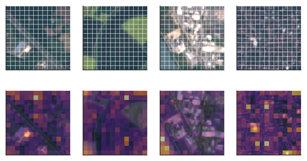
Chart: Patches and attention on real EuroSAT images

Patch grid and class-token attention (attention rollout) of CLIP ViT-B/16 on four EuroSAT test images.

Source: EuroSAT, Sentinel-2 images (Helber et al., 2019). Data: 4 test images upscaled to 224 x 224 pixels = 14 x 14 patches of 16 x 16; model CLIP ViT-B/16.

The attention rollout multiplies the head-averaged attention matrices of all layers, with the identity added for the residual connection (Abnar & Zuidema, 2020).

CLIP: images and text in one space

CLIP learns by matching images with their captions

Slide 12 in the PDF
\[s_{ij}=\frac{\mathbf u_i^{\top}\mathbf v_j}{\tau},\qquad \mathcal L=-\frac{1}{2n}\sum_{i=1}^{n}\Big[\log\frac{e^{s_{ii}}}{\sum_j e^{s_{ij}}}+\log\frac{e^{s_{ii}}}{\sum_j e^{s_{ji}}}\Big]\]

where \(\mathbf u_i\) and \(\mathbf v_j\) are the normalised image and text embeddings and \(\tau\) a learned temperature (Radford et al., 2021). The ViT-B/32 model has 151.3 million parameters and the ViT-B/16 model has 149.6 million.

Zero-shot classification

Slide 13 in the PDF

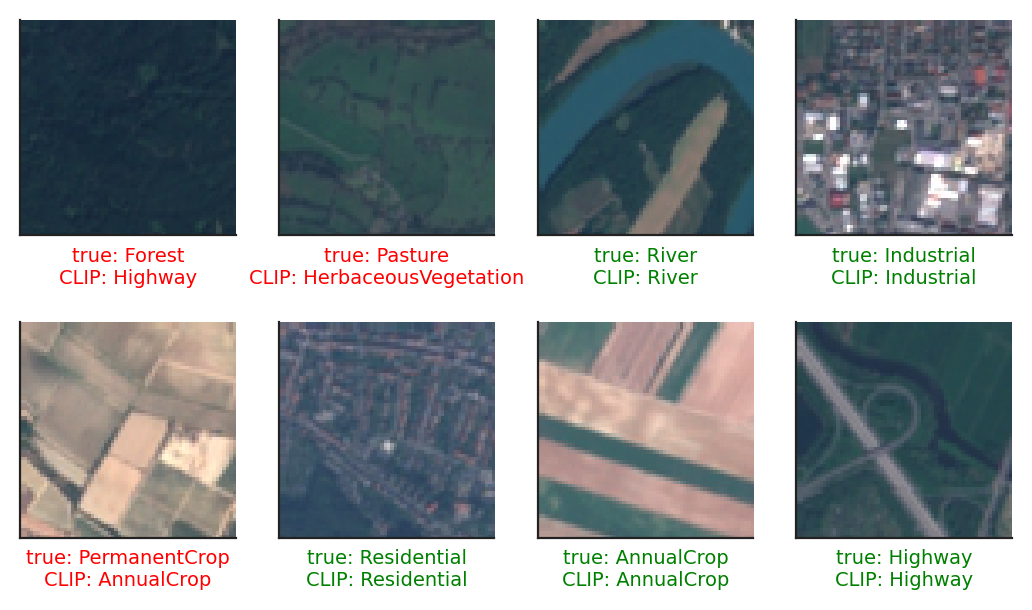
Each class is described by sentences such as "a satellite photo of {class}."; their averaged text embedding \(\mathbf w_c\) becomes the weight vector of the class, and the image goes to the class with the largest cosine similarity. The best zero-shot model, CLIP ViT-B/16 with an ensemble of five templates, classifies 56.4 % of the test images correctly, against 10 % by chance.

The words in the prompt change the accuracy

Slide 14 in the PDF
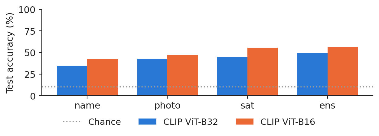
Chart: The words in the prompt change zero-shot accuracy

Zero-shot accuracy for four prompt designs and two CLIP models.

Source: EuroSAT, Sentinel-2 images (Helber et al., 2019). Data: 5400 test images, no training.

With the bare folder names, ViT-B/16 reaches 42.4 %; "a satellite photo of" lifts it to 55.4 % and the five-template ensemble to 56.4 %. Telling the model what kind of picture it sees matters more than the size of the model.

Zero-shot errors

Slide 16 in the PDF
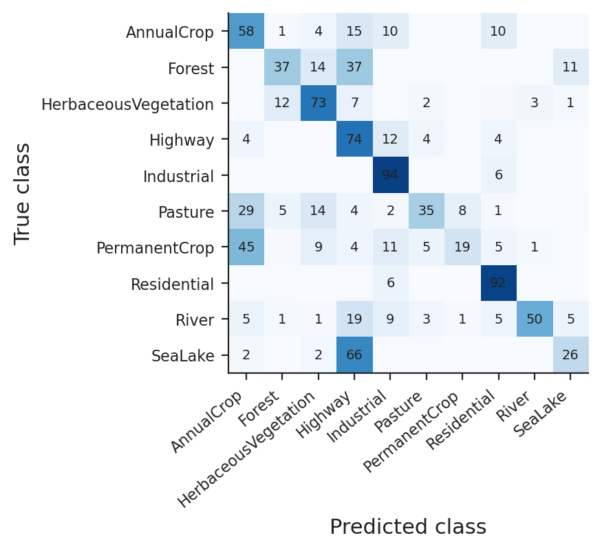
Chart: Zero-shot errors on visually similar land uses

Confusion matrix of the best zero-shot model, row percentages.

Source: EuroSAT, Sentinel-2 images (Helber et al., 2019). Data: 5400 test images; row percentages.

Industrial and residential areas are recognised in more than nine cases out of ten (93.6 % and 92.3 %), but permanent crops only in 18.6 % of cases, and 399 of the 600 sea-or-lake images were called highway. Look-alike classes need examples.

Text-to-image search

Slide 17 in the PDF

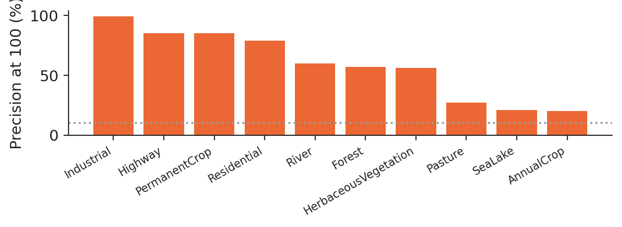
The same embeddings, used the other way round, turn a sentence into an image search: on average 58.9 % of the 100 images closest to a class prompt truly belong to the class, from 99.0 % for industrial areas to 20.0 % for annual crops. Searching first and labelling the hits is the cheapest way to build a labelled image set.

A linear probe on CLIP features

Slide 18 in the PDF

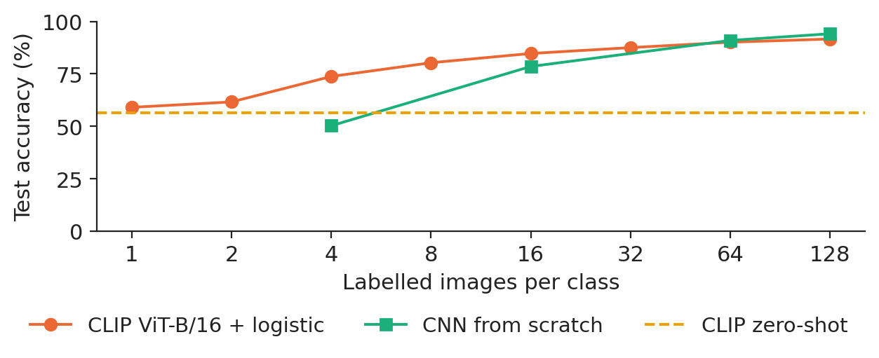
Keeping CLIP frozen and training only a logistic regression on its image embeddings already beats zero-shot with one labelled image per class (59.0 %), and reaches 95.5 % with all 21,600 training images.

Pre-trained features and the number of labels

Slide 19 in the PDF
Chart: Pre-trained features and a CNN trained from scratch, by number of labels

Test accuracy against labelled images per class: CLIP probe, CNN from scratch, zero-shot.

Source: EuroSAT, Sentinel-2 images (Helber et al., 2019). Data: 5400 test images; shaded = range over seeds.

With 16 labelled images per class the probe reaches 84.7 % against 78.5 % for a CNN trained from scratch; from about 64 per class the CNN catches up, and with 128 it is ahead (94.1 % against 91.6 %). On all training images the CNN reaches 97.4 %. Foundation models pay off when labels are scarce.

Size and speed

Slide 20 in the PDF

The CNN has 289.2 thousand parameters; CLIP ViT-B/32 embeds an image in 4.23 ms on a laptop and ViT-B/16 in 20.49 ms; the VLM needs about 262 ms per image and question.

Vision-language models: reading charts and tables

A VLM: an image encoder connected to a language model

Slide 22 in the PDF
\[\mathbf H_v=\mathbf W_p\,f_{\text{ViT}}(I),\qquad p(y_t\mid y_{<t},I,q)=\mathrm{LLM}_{\boldsymbol\theta}\big([\mathbf H_v;\ \mathbf e(q);\ \mathbf e(y_{<t})]\big)\]

Image patches are projected into the word-embedding space of a large language model (LLM), which reads them as extra tokens (Liu et al., 2023). We use Qwen2-VL-2B-Instruct, with 2.21 billion parameters (Wang et al., 2024).

Market regimes as a visual recognition task

Slide 23 in the PDF

Following Jheng, Pele, Tak and Găman (2026), each window of 120 trading days of the S&P 500 is drawn as a two-panel image (price and drawdown) and labelled "stress" when the 20-day volatility at its end exceeds its rolling 90th percentile of the previous three years. Models are trained on windows up to 2018 and tested on 394 windows from 2019, where the stress share is 8.4 %.

Stress detection from charts and from numbers

Slide 24 in the PDF
Chart: Detecting market stress from charts and from numbers

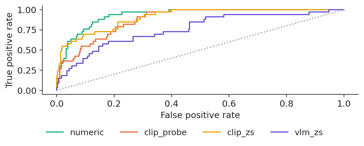
A calm and a stress window, and the ROC curves of four detectors on the test years.

Source: Yahoo Finance, daily quotes. Data: S&P 500, windows of 120 trading days every 5 days; test 7 Jan 2019 to 30 Oct 2026.

The area under the receiver operating characteristic curve (AUC) is 0.933 for logistic regression on returns, volatility and drawdown, 0.907 for CLIP zero-shot, 0.880 for logistic regression on CLIP image embeddings and 0.758 for Qwen2-VL zero-shot.

Discrimination and precision

Slide 25 in the PDF

Average precision, which matters for a rare event, is 0.578 for the numbers, 0.605 for CLIP zero-shot, 0.449 for the CLIP probe and 0.302 for the VLM. When the numbers exist, a picture adds a lossy step; images earn their place when numbers are missing.

Reading charts and tables with a small VLM

Slide 26 in the PDF

Asked whether the price ended higher or lower over the window, the VLM is right in 57.1 % of 394 charts at the 0.5 threshold, below the 74.9 % of always answering the majority, yet its AUC is 0.974: the ranking is right and the threshold is biased, so recalibration on validation charts fixes most of the problem. Reading the 10-year yield from 60 rendered tables, it gives the exact value in 25.0 % of cases, with a mean absolute error of 0.192 percentage points.

A document pipeline in a bank

Slide 27 in the PDF

Known templates go to a rule-based parser; optical character recognition and layout analysis handle text and tables; a VLM reads free-form pages and charts; checks on totals, dates and ranges send failures to a person; and an exact-match rate per field is measured on a labelled sample.

Synthesis of the course

Methods of the course by data type

Slide 30 in the PDF

Tables (lectures 1–3), images (4, 14), sequences (5, 13), text (6, 7, 12), generation (8), graphs (9), decisions (10) and trust (11): each data type has its architecture, and every lecture compared it with a benchmark on real data.

Choosing a model

Slide 31 in the PDF

Start with the decision and the cost of errors, fit the benchmark first, count the labels (few labels: a foundation model zero-shot or with a probe; many labels: a trained network), match the architecture to the data, and prove the result with a test, several seeds, calibration and an explanation.

Five evaluation rules

Slide 32 in the PDF

No leakage; a benchmark next to every network; seeds and intervals; metrics for rare events; real data and reproducible scripts.

Foundation models for images, text and time series

Slide 33 in the PDF

The same pattern, pre-train once and use zero-shot or with a small head, worked for text (Lecture 12), time series (Lecture 13) and images (this lecture: 56.4 % zero-shot, 95.5 % with a probe on all labels). The common caveat is that pre-training data may contain the test set.

Responsible use

Slide 36 in the PDF

The European Union Artificial Intelligence Act lists credit scoring among high-risk uses; a model card documents data, period, metric, benchmark, seeds and known failure cases; models are re-tested on new data; local open models keep client data in-house.

Section summary

Multimodal models label and search images without labels and read charts and tables imperfectly; with numbers available, numbers win. Across the course, the same discipline applies: benchmark first, real data, no leakage, several seeds, a test, an explanation.

Videos: the intuition behind the mathematics (in English)

Abbreviations

ASEBucharest University of Economic Studies
AUCarea under the receiver operating characteristic curve
CLIPcontrastive language–image pre-training
CNNconvolutional neural network
ECBEuropean Central Bank
ESGenvironmental, social and governance
GANgenerative adversarial network
GNNgraph neural network
GPTgenerative pre-trained transformer
ICBEInternational Conference on Business Excellence
InfoNCEinformation noise-contrastive estimation loss
IPEInstitute for Economic Forecasting, Romanian Academy
LLaVAlarge language and vision assistant
LLMlarge language model
LSTMlong short-term memory network
MLPmultilayer perceptron
OCRoptical character recognition
RAGretrieval-augmented generation
RGBred, green, blue (colour channels)
RLreinforcement learning
ROCreceiver operating characteristic
SHAPShapley additive explanations
VAEvariational autoencoder
VaRValue-at-Risk
ViTvision transformer
VLMvision-language model
XAIexplainable artificial intelligence

References

  • Abnar, S. & Zuidema, W. (2020). Quantifying attention flow in transformers. Proceedings of the 58th Annual Meeting of the Association for Computational Linguistics, 4190–4197. doi:10.18653/v1/2020.acl-main.385
  • Bishop, C. M. & Bishop, H. (2024). Deep Learning: Foundations and Concepts. Springer. doi:10.1007/978-3-031-45468-4
  • Diaconu, D. & Pele, D. T. (2026). Explainable AI in financial fraud detection: Evidence from the IEEE-CIS fraud dataset. Proceedings of the International Conference on Business Excellence, 20(1), 118–132. doi:10.2478/picbe-2026-0015
  • Dosovitskiy, A. et al. (2021). An image is worth 16x16 words: Transformers for image recognition at scale. International Conference on Learning Representations. arXiv:2010.11929
  • Găman, Ș., Tak, R., Jheng, S.-L. & Pele, D. T. (2026). ESG-aware asset selection and portfolio optimization: A comparative study of multi-criteria decision-making methods. Proceedings of the International Conference on Business Excellence, 20(1), 133–147. doi:10.2478/picbe-2026-0016
  • Helber, P., Bischke, B., Dengel, A. & Borth, D. (2019). EuroSAT: A novel dataset and deep learning benchmark for land use and land cover classification. IEEE Journal of Selected Topics in Applied Earth Observations and Remote Sensing, 12(7), 2217–2226. doi:10.1109/JSTARS.2019.2918242
  • Jheng, S.-L., Pele, D. T., Tak, R. & Găman, Ș. (2026). A multimodal vision-language framework for financial anomaly detection. Proceedings of the International Conference on Business Excellence, 20(1), 191–201. doi:10.2478/picbe-2026-0020
  • Liu, H., Li, C., Wu, Q. & Lee, Y. J. (2023). Visual instruction tuning. Advances in Neural Information Processing Systems, 36. arXiv:2304.08485
  • Oord, A. van den, Li, Y. & Vinyals, O. (2018). Representation learning with contrastive predictive coding. arXiv:1807.03748
  • Pele, D. T., Bolovăneanu, V., Lin, M.-B., Ren, R., Ginavar, A. T., Spilak, B., Andrei, A.-V., Toma, F.-M., Lessmann, S. & Härdle, W. K. (2026). In the beginning was the Word: LLM-VaR and LLM-ES. Expert Systems with Applications, 295, 128676. doi:10.1016/j.eswa.2025.128676
  • Radford, A. et al. (2021). Learning transferable visual models from natural language supervision. Proceedings of the 38th International Conference on Machine Learning, 8748–8763. arXiv:2103.00020
  • Wang, P. et al. (2024). Qwen2-VL: Enhancing vision-language model's perception of the world at any resolution. arXiv:2409.12191

Text written for the web version of the lecture; numbers, charts and sources come from the slides and their Quantlets.