Neural Networks and Deep Learning

Lecture 7: Attention and transformers

Lecture 7

Attention and transformers

Prof. dr. Daniel Traian PELE

Bucharest University of Economic Studies (ASE), Department of Statistics and Econometrics
Romanian Academy, Institute for Economic Forecasting (IPE)

Every trading desk, credit team and central-bank watcher reads text: news, posts, reports, speeches. Since 2017 almost every machine that reads text at scale has been built from the same component, the transformer, whose core operation is attention: every word looks at every other word and decides how much of it to borrow.

This lecture writes attention and the transformer block with every symbol defined, and tests them on 9,543 labelled finance tweets: a small transformer trained from scratch, a pretrained BERT model for finance (FinBERT) used as is, frozen and fine-tuned, and a term frequency–inverse document frequency (TF-IDF) benchmark. The result is a lesson in where the power of transformers comes from: pretraining.

What you will be able to do

  • Explain why attention replaced recurrence for text: one step between any two words, computed in parallel.
  • Write scaled dot-product attention, multi-head attention, positional encoding and the transformer block.
  • Compare a transformer from scratch, FinBERT and a TF-IDF benchmark on real finance tweets, with bootstrap intervals.
  • Read attention maps with care and decide when pretraining, fine-tuning or a simple model is the right choice.

Lecture plan

  1. Motivation for the attention mechanismText arrives fast and carries information that prices react to; recurrent networks read it slowly and forget.
  2. The attention mechanismQueries, keys and values; scaling; several heads; and what attention maps do and do not show.
  3. The transformer architecturePositions, the block, the two families and the tokenizer.
  4. Case study: sentiment of finance tweetsSeven models on one held-out test set, with bootstrap intervals and per-class errors.
  5. Transformers in practiceFrom scores to signals, long documents, and transformers beyond text.

Motivation for the attention mechanism

Text arrives fast and carries information that prices react to; recurrent networks read it slowly and forget.

Financial news as input for models

Slide 5 in the PDF

A sentiment model maps a text \(x_{1:n}\) to a fixed-size representation \(\mathbf h\) and then to the probabilities of three classes, \(\hat{\mathbf p}=\operatorname{softmax}(W_o\mathbf h+\mathbf b_o)\); the whole lecture is about how to compute \(\mathbf h\). Our data are finance tweets labelled bearish, bullish or neutral: 9,543 for training and 2,388 for the test, of which 14.5 % bearish, 19.9 % bullish and 65.6 % neutral. Media pessimism predicts next-day returns and trading volume (Tetlock, 2007), so such a model is a measurement instrument.

In practice: a sentiment model must be accurate on the rare bearish news, not only on average.
Limits of recurrent networks for long texts

Slide 6 in the PDF

A recurrent network updates one state vector token by token, \(\mathbf h_t=\phi(W_h\mathbf h_{t-1}+W_x\mathbf x_t+\mathbf b)\), so the gradient between words 1 and \(n\) is a product of \(n-1\) Jacobians that shrinks or explodes with the distance. The path between words \(i\) and \(j\) has \(|i-j|\) steps, and the \(n\) steps cannot run in parallel. The long short-term memory (LSTM) of Lecture 5 eases the first problem but keeps the second. In “profit fell, but guidance was raised”, the verdict depends on a word far from the subject.

Length of tweets and central-bank speeches in tokens

Slide 7 in the PDF

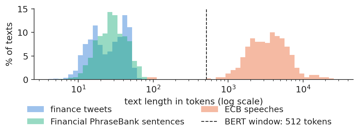
In WordPiece tokens, the median tweet has 25 tokens, the median Financial PhraseBank sentence 28 and the median speech of the European Central Bank (ECB) 3,338. Of the 400 speeches, 98.8 % exceed the 512-token window of BERT; only 0.19 % of the tweets exceed 64 tokens.

Chart: Length of tweets and central-bank speeches in tokens

Length in tokens of finance tweets, Financial PhraseBank sentences and ECB speeches, log scale.

Source: Twitter financial news (zeroshot); Malo et al. (2014); European Central Bank speeches; tokenizer of the ProsusAI model. Data: finance tweets; Financial PhraseBank; European Central Bank speeches 8 Jan 2022 to 30 Oct 2026.

In practice: match the model to the text length: a tweet fits any transformer, a speech needs chunking or a long-context model.

Section summary

Recurrence links distant words through long sequential paths; attention links every pair in one step.

The attention mechanism

Queries, keys and values; scaling; several heads; and what attention maps do and do not show.

Attention is a soft dictionary lookup

Slide 9 in the PDF

Each token \(i\) asks a question \(\mathbf q_i=W_Q^\top\mathbf x_i\), every token \(j\) offers a key \(\mathbf k_j=W_K^\top\mathbf x_j\) and a value \(\mathbf v_j=W_V^\top\mathbf x_j\), and the output is

\[\mathbf y_i=\sum_{j=1}^n a_{ij}\mathbf v_j,\qquad a_{ij}=\frac{\exp(\mathbf q_i^\top\mathbf k_j/\sqrt{d_k})}{\sum_{l}\exp(\mathbf q_i^\top\mathbf k_l/\sqrt{d_k})}.\]
(7.1)

A dictionary returns the value of the one matching key; attention returns a blend of all values, weighted by how well the keys match. The blend is differentiable, so the projections are learned, and any two words are one step apart.

In practice: each output word is a context-aware mixture: “guidance” can borrow meaning from “raised” ten words later.

Attention in matrix form for all words at once

Slide 10 in the PDF

Stacking the tokens in \(X\in\mathbb R^{n\times d}\) gives \(\operatorname{Attention}(Q,K,V)=\operatorname{softmax}(QK^\top/\sqrt{d_k}+\mathbf M)V\), with a mask \(\mathbf M\) equal to \(-\infty\) for padding or, in a decoder, for future tokens. The cost per layer is \(O(n^2d)\) operations and \(O(n^2)\) memory: attention over a median ECB speech costs about 17,828 times that over a median tweet. In exchange there is no loop over positions, and graphics processors multiply the whole sentence at once.

Scaling by √d_k and saturation of the softmax

Slide 11 in the PDF

If the entries of \(\mathbf q\) and \(\mathbf k\) are independent with mean 0 and variance 1, then \(\operatorname{Var}(\mathbf q^\top\mathbf k)=d_k\). With \(d_k=64\), as in each head of BERT, raw scores have a standard deviation of 8, so one word takes almost all the weight and the softmax Jacobian \(\operatorname{diag}(\mathbf a)-\mathbf a\mathbf a^\top\) is close to zero: the queries and keys stop learning. Dividing by \(\sqrt{d_k}\) restores unit variance for every \(d_k\).

Multi-head attention: several relations at once

Slide 12 in the PDF

Multi-head attention runs \(h\) attentions with projections of size \(d/h\) and concatenates them: \(\operatorname{MHA}(X)=[\mathbf H_1\|\cdots\|\mathbf H_h]W_O\), with \(4d^2\) parameters, the same as one large head. BERT-base has 12 layers of 12 heads with \(d\) = 768 and 64 dimensions per head; our small transformer has 2 layers of 4 heads with \(d=64\).

What FinBERT attends to in a real bearish tweet

Slide 13 in the PDF

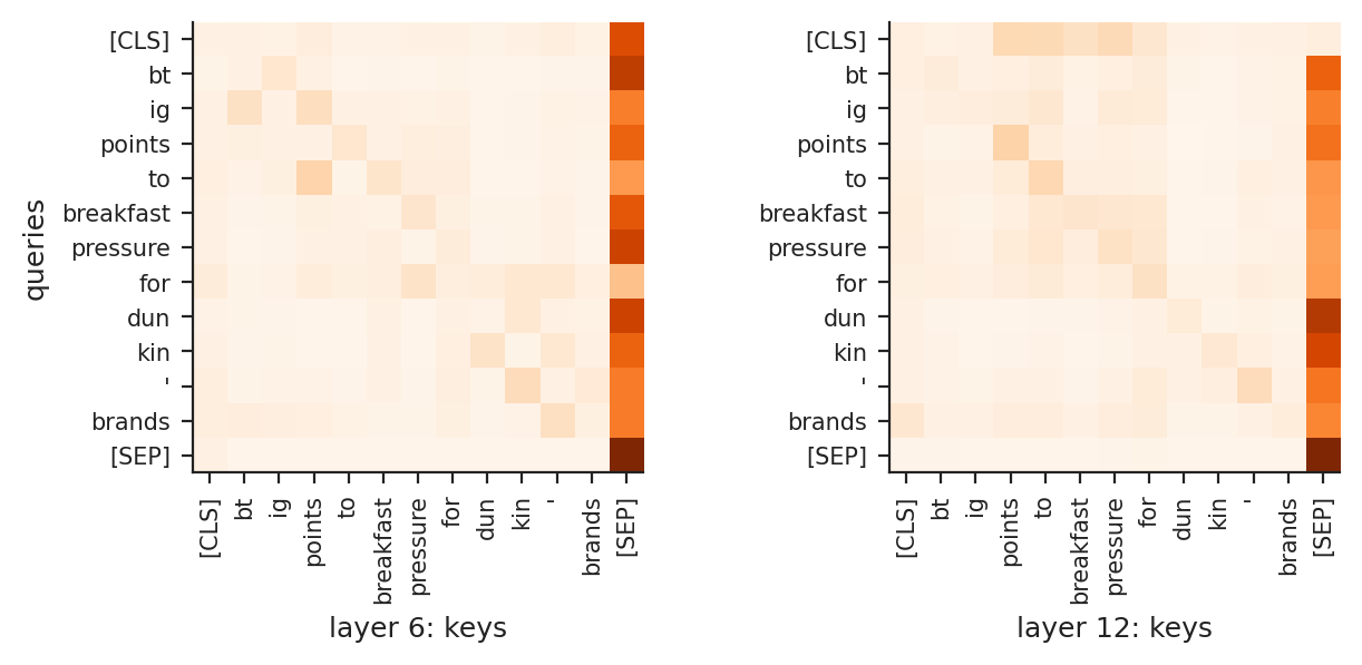
For the bearish test tweet shown, pretrained FinBERT gives only 7.3 % probability of negative: the bearish tone is implicit, and the zero-shot model misses it. In layer 6 the summary token [CLS] puts 5.7 % of its attention on “points”; in layer 12 most of the weight flows to the separator tokens.

Chart: What FinBERT attends to in a real bearish tweet

Attention of pretrained FinBERT, averaged over the 12 heads, layers 6 and 12; rows are queries, columns keys.

Source: Twitter financial news datasets (Hugging Face, zeroshot). Data: one test tweet; pretrained FinBERT, attention averaged over 12 heads.

Across layers, attention becomes concentrated on separator tokens

Slide 14 in the PDF

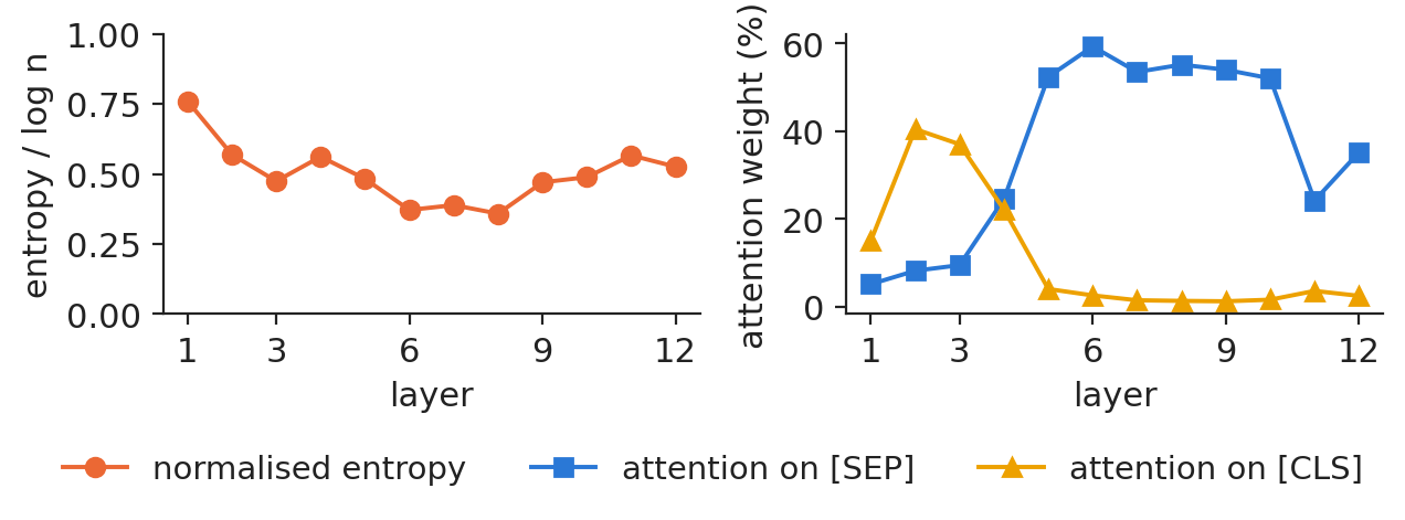
Over 500 test tweets, the entropy of the attention rows divided by \(\log n\) is 0.76 in layer 1 and falls to 0.36 in layer 8 (1 would be uniform attention). Up to 59.3 % of all attention (layer 6) goes to the separator [SEP], a “no-op” that a head uses when it has nothing to add (Clark et al., 2019).

Chart: Across layers, attention becomes concentrated on separator tokens

Normalised entropy of attention and share of attention on [CLS] and [SEP], by layer of FinBERT.

Source: Twitter financial news datasets (Hugging Face, zeroshot). Data: 500 test tweets; pretrained FinBERT.

Attention weights as explanations: limitations

Slide 15 in the PDF

The contribution of word \(j\) to word \(i\) is \(a_{ij}\) times a value vector whose norm can be large or small, and the residual stream carries information that attention never touches. Different attention maps can give the same prediction (Jain and Wallace, 2019), and heavy attention on [SEP] carries almost no information. Gradient-based attributions and occlusion tests (Lecture 11) are better tools.

In practice: never show an attention map to a regulator as “the reason” for a decision.

Section summary

Attention = softmax of scaled query–key scores times values; heads specialise; attention maps are clues, not explanations.

The transformer architecture

Positions, the block, the two families and the tokenizer.

Sinusoidal positional encoding

Slide 17 in the PDF

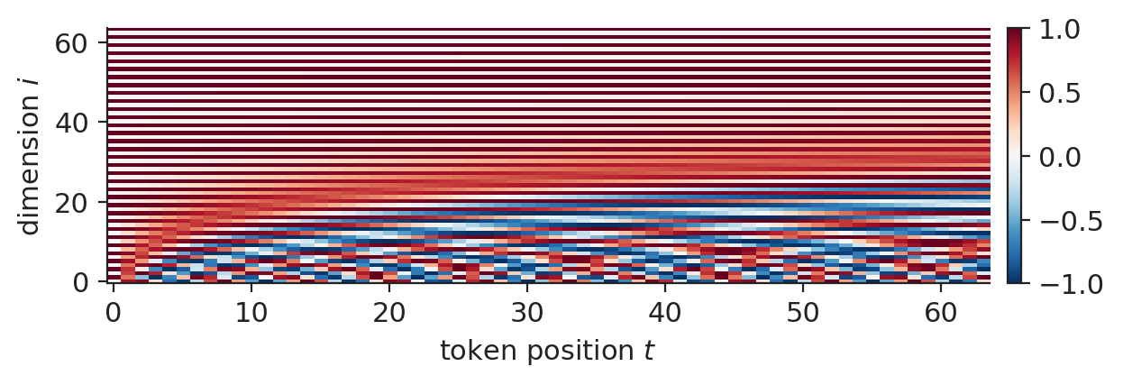
Self-attention is permutation-equivariant: without positions, “rates cut, stocks up” would equal “stocks cut, rates up”. The original transformer adds to each token embedding the vector \(p_{t,2i}=\sin(t/10000^{2i/d})\), \(p_{t,2i+1}=\cos(t/10000^{2i/d})\); low dimensions change fast with the position, high ones slowly, so every position has a unique code and relative shifts are linear maps.

Chart: Sinusoidal positional encoding

Sinusoidal positional encoding for 64 positions and 64 dimensions (mechanism illustration).

Source: Vaswani et al. (2017), sinusoidal formula. Data: mechanism illustration, d=64, 64 positions.

A transformer block: attention, feed-forward, residuals, normalisation

Slide 18 in the PDF

In the pre-norm form a block computes

\[Z=X+\operatorname{MHA}(\operatorname{LN}(X)),\qquad X'=Z+\operatorname{FFN}(\operatorname{LN}(Z)),\]
(7.2)

where the position-wise feed-forward network (FFN) is \(W_2\,\mathrm{GELU}(W_1\mathbf z+\mathbf b_1)+\mathbf b_2\) with the Gaussian error linear unit (GELU), and LN is layer normalisation over the features of one token. A block has about \(12d^2\) parameters, two thirds of them in the feed-forward part. Our block has \(d=64\), an FFN of width 128 and dropout 0.1; two blocks have 67,139 parameters outside the embeddings.

Encoders and decoders: two pretraining objectives

Slide 19 in the PDF

Bidirectional Encoder Representations from Transformers (BERT) is pretrained by masked language modelling (MLM): 15 % of the tokens are hidden and predicted from both sides. The Generative Pre-trained Transformer (GPT) predicts the next token with a causal mask, \(M_{ij}=-\infty\) for \(j>i\), and today's large language models (LLM) follow this design. Encoders suit classification and extraction, decoders generation; the original transformer had both, for translation.

In practice: for labelling texts use an encoder; for writing reports use a decoder (Lecture 12).

Subword tokenisation of text

Slide 20 in the PDF

A WordPiece tokenizer splits rare words into frequent pieces, so a fixed vocabulary, 30,522 pieces for FinBERT, covers any word, including tickers and new company names. The text becomes [CLS], the pieces and [SEP], and each token gets its embedding plus a position and a segment vector. Our tweets have a median of 25 tokens, a 99th percentile of 57 and a maximum of 82; we cut at 64 tokens. In small models the embedding table dominates: our small transformer has 2,020,547 parameters, only 67,139 outside the table.

Attention, recurrence and convolution compared

Slide 21 in the PDF
LayerCost per layerSequential stepsLongest path
Self-attention\(O(n^2d)\)\(O(1)\)\(O(1)\)
Recurrent\(O(nd^2)\)\(O(n)\)\(O(n)\)
Convolution, kernel \(k\)\(O(knd^2)\)\(O(1)\)\(O(\log_kn)\)

A recurrent neural network (RNN) is cheap per step but slow per sentence; a convolutional neural network (CNN) is parallel but needs depth to link distant words; self-attention has a constant path and full parallelism, paid with \(n^2\) memory, which for tweets of about 25 tokens is negligible.

Section summary

A transformer stacks attention and feed-forward blocks with residuals and normalisation; positions are added, tokens are subwords.

Case study: sentiment of finance tweets

Seven models on one held-out test set, with bootstrap intervals and per-class errors.

Seven models evaluated on a common test set

Slide 23 in the PDF

The published training tweets are split into 8,588 for training and 955 for validation (10 %, stratified); the published validation set is our test set of 2,388 tweets, used once. The models are a TF-IDF logistic regression on word 1–2-grams (17,119 features); a mean of learned token embeddings without attention; our small transformer, with and without positions; and FinBERT, a BERT model further trained on financial text (Araci, 2019), used zero-shot, frozen with a logistic regression on its 768-dimensional vectors, and fine-tuned. We do not test on Financial PhraseBank: FinBERT was fine-tuned on it, so the test would be contaminated.

Our small transformer, trained from scratch

Slide 24 in the PDF

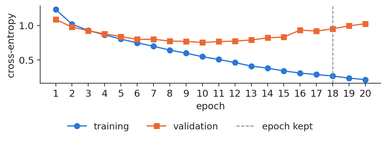
Two blocks sit on top of the token and position embeddings; the outputs are averaged over the real tokens and passed to a linear layer with three classes, trained with class-weighted cross-entropy, Adam with decoupled weight decay (AdamW), learning rate \(5\cdot10^{-4}\) and early stopping on the validation macro-F1, the mean of the three per-class F1 scores. The model has 2,020,547 parameters and trains in about 44 seconds per seed. For seed 1 the validation loss is lowest at epoch 10 and then rises, while the validation macro-F1 still peaks at epoch 18: the model becomes overconfident before it stops improving.

Chart: The small transformer overfits: the validation loss turns up after a few epochs

Training and validation cross-entropy by epoch, seed 1; the dashed line marks the epoch kept.

Source: Twitter financial news datasets (Hugging Face, zeroshot). Data: own estimates; small transformer, seed 1.

In practice: macro-F1 is the right yardstick when the rare class, bearish news, is the one that costs money.

Comparison of the models: macro-F1 on the test set

Slide 26 in the PDF

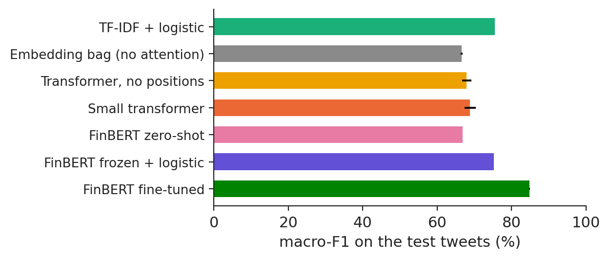
On the 2,388 test tweets, macro-F1 is 84.8 % for fine-tuned FinBERT, 75.5 % for TF-IDF and 68.8 % for the small transformer (standard deviation 1.5 over 3 seeds). FinBERT without any training on tweets reaches 66.9 %, and frozen FinBERT with a logistic regression 75.3 %.

Chart: Comparison of the models: macro-F1 on the test set

Macro-F1 on the test tweets, mean over the seeds with the standard deviation.

Source: Twitter financial news datasets (Hugging Face, zeroshot). Data: own estimates; 2,388 test tweets (published validation split).

The bearish class is where models differ most

Slide 27 in the PDF

Fine-tuned FinBERT finds 82.9 % of the bearish tweets with a precision of 77.9 %; TF-IDF finds 70.3 % with 63.5 %, and the small transformer 59.7 % with 51.1 %.

In practice: report per-class recall and precision: an average can hide a model that misses the news that matter.

Paired bootstrap test of the differences on the test tweets

Slide 28 in the PDF

Resampling the test tweets 1,000 times, with the same draw for both models, gives these differences in macro-F1 (percentage points, 95 % interval): fine-tuned FinBERT minus TF-IDF +9.3 [+7.3; +11.3]; small transformer minus TF-IDF −6.6 [−8.3; −4.9]; frozen FinBERT minus TF-IDF −0.2 [−2.5; +2.0].

In practice: an interval that excludes zero is the minimum evidence before replacing a production model.

With little labelled data, pretrained representations matter most

Slide 29 in the PDF

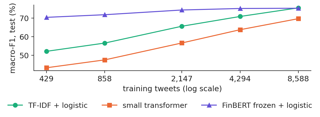
With only 429 training tweets, frozen FinBERT with a logistic regression reaches 70.4 % macro-F1, TF-IDF 52.1 % and the small transformer 43.3 %. Pretraining is data you did not have to label: billions of words already shaped the FinBERT vectors, whereas a model from scratch must learn the language and the task at once.

Chart: With little labelled data, pretrained representations matter most

Test macro-F1 by number of training tweets (seed 1).

Source: Twitter financial news datasets (Hugging Face, zeroshot). Data: own estimates; 2,388 test tweets (published validation split).

Zero-shot errors corrected by fine-tuning

Slide 30 in the PDF

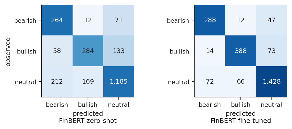
FinBERT was trained on sentences from news, not on tweets. Without training on tweets it finds 264 of the 347 bearish test tweets; after fine-tuning it finds 288. The remaining errors are mostly confusions with the neutral class: 47 bearish and 73 bullish tweets read as neutral, and only 12 bearish tweets read as bullish.

Chart: Zero-shot errors corrected by fine-tuning

Confusion matrices of FinBERT on the test tweets, zero-shot and fine-tuned (seed 1).

Source: Twitter financial news datasets (Hugging Face, zeroshot). Data: own estimates; 2,388 test tweets (published validation split).

Fine-tuning: pretrained initial weights and small learning rates

Slide 31 in the PDF

Fine-tuning starts from \(\boldsymbol\theta_0=\boldsymbol\theta_{\text{FinBERT}}\) and moves all 109.5 million weights with a small learning rate, \(2\cdot10^{-5}\) decaying linearly over 3 epochs; the epoch with the best validation macro-F1 is kept. It gains +17.9 points over the zero-shot model and +9.3 over TF-IDF, at a cost of about 5.2 minutes per seed on the graphics processor of a laptop. Too large a learning rate erases what pretraining learnt (catastrophic forgetting).

In practice: fine-tuning a pretrained encoder is today's default for any labelled text task with a few thousand examples.

Role of word order in tweet classification

Slide 32 in the PDF

The same small transformer reaches 68.8 % macro-F1 with positions and 67.9 % without them, a difference of +0.9 points with a bootstrap interval of [+0.1; +1.7]; the mean of embeddings without any attention reaches 66.6 %. Short, formulaic tweets are mostly bags of signal words; order matters for negation, contrast, long documents and numbers attached to the right entity.

In practice: test the simple version of your model first: on short texts much of the transformer's power is unused.

Section summary

Pretraining decides: fine-tuned FinBERT leads, TF-IDF is a strong benchmark, and a transformer from scratch needs far more data.

Transformers in practice

From scores to signals, long documents, and transformers beyond text.

Sentiment scores as a business signal

Slide 34 in the PDF

A production pipeline streams news and posts through the tokenizer and a fine-tuned encoder, then aggregates the class probabilities by firm and day, for example the share of bearish minus bullish messages weighted by reach. Such signals serve risk monitoring of a credit portfolio, early warning for issuers or an overlay on Value-at-Risk (VaR). The pitfalls are look-ahead (use only texts time-stamped before the decision), domain shift (a model of news sentences misreads tweets), label noise, sarcasm and drift in market vocabulary.

In practice: a sentiment score is an input to a model, not a trading decision: backtest it before use.

Long documents: central-bank speeches and annual reports

Slide 35 in the PDF

Our 400 ECB speeches, from 8 Jan 2022 to 30 Oct 2026, have a median of 3,338 tokens and up to 22,646. The options are chunking into windows of 512 tokens and pooling the chunk scores, hierarchical models with attention over sentence vectors, and long-context models with sparse or memory-efficient attention.

In practice: for a monetary-policy desk, chunking plus a well-tested encoder usually beats an untested long-context model.

Transformers for data other than text

Slide 36 in the PDF

Patches of a time series become tokens in pretrained forecasting models (Lecture 13); columns or past payments become tokens for tabular and transaction data; attention restricted to the edges of a graph is the graph attention network (Lecture 9); image patches become tokens in vision-language models that read charts and reports (Lecture 14).

In practice: whatever the data, the question is the same: what are the tokens, and which pairs may attend to each other?

Explore it visually

Free interactive tools and illustrated guides for this lecture; most run in the browser.

  • Transformer Explainer: a GPT-2 model running in the browser: type a sentence, open one attention head to see the scores \(\mathbf q^{\top}\mathbf k\), the softmax and the weighted sum of the values; move the temperature to sharpen or flatten the next-token distribution.
  • LLM Visualization (B. Bycroft): a 3D walk through a small GPT, block by block: every matrix product of normalisation, attention and the feed-forward layer.
  • The Illustrated Transformer (J. Alammar): queries, keys and values drawn step by step for one sentence.
  • Attention variants (S. Raschka): from multi-head to grouped-query and latent attention, sliding windows and sparse attention: how recent models reduce the memory of keys and values.

Section summary

Use transformers as measurement instruments: time-stamp the inputs, chunk long texts, and backtest the signal.

Videos: the intuition behind the mathematics (in English)

Abbreviations

ASEBucharest University of Economic Studies
BERTBidirectional Encoder Representations from Transformers
CNNconvolutional neural network
ECBEuropean Central Bank
ESexpected shortfall
FFNposition-wise feed-forward network
FinBERTBERT further trained on financial text
GELUGaussian error linear unit
GPTGenerative Pre-trained Transformer
IPEInstitute for Economic Forecasting, Romanian Academy
LLMlarge language model
LNlayer normalisation
LSTMlong short-term memory network
MHAmulti-head attention
MLMmasked language modelling
MPSMetal Performance Shaders (Apple graphics processor back end)
NLPnatural language processing
ReLUrectified linear unit
RNNrecurrent neural network
TF-IDFterm frequency–inverse document frequency
VaRValue-at-Risk

References

  • Araci, D. (2019). FinBERT: Financial sentiment analysis with pre-trained language models. arXiv:1908.10063
  • Ba, J. L., Kiros, J. R. & Hinton, G. E. (2016). Layer normalization. arXiv:1607.06450
  • Bahdanau, D., Cho, K. & Bengio, Y. (2015). Neural machine translation by jointly learning to align and translate. International Conference on Learning Representations. arXiv:1409.0473
  • Bishop, C. M. & Bishop, H. (2024). Deep Learning: Foundations and Concepts, ch. 12. Springer. doi:10.1007/978-3-031-45468-4
  • Clark, K., Khandelwal, U., Levy, O. & Manning, C. D. (2019). What does BERT look at? An analysis of BERT's attention. BlackboxNLP Workshop, 276–286. doi:10.18653/v1/W19-4828
  • Devlin, J., Chang, M.-W., Lee, K. & Toutanova, K. (2019). BERT: Pre-training of deep bidirectional transformers for language understanding. Proceedings of NAACL, 4171–4186. doi:10.18653/v1/N19-1423
  • Efron, B. & Tibshirani, R. J. (1993). An Introduction to the Bootstrap. Chapman & Hall. doi:10.1201/9780429246593
  • Jain, S. & Wallace, B. C. (2019). Attention is not explanation. Proceedings of NAACL, 3543–3556. doi:10.18653/v1/N19-1357
  • Jheng, S.-L., Tak, R., Găman, Ș., Mazurencu-Marinescu-Pele, M. & Pele, D. T. (2026). Can foundation models manage risk? Zero-shot VaR and ES forecasting with conformal calibration in CEE markets. Economic Computation and Economic Cybernetics Studies and Research, 60(2), 267–290. doi:10.24818/18423264/60.2.26.14
  • Loshchilov, I. & Hutter, F. (2019). Decoupled weight decay regularization. International Conference on Learning Representations. arXiv:1711.05101
  • Malo, P., Sinha, A., Korhonen, P., Wallenius, J. & Takala, P. (2014). Good debt or bad debt: Detecting semantic orientations in economic texts. Journal of the Association for Information Science and Technology, 65(4), 782–796. doi:10.1002/asi.23062
  • Pele, D. T., Bolovăneanu, V., Lin, M.-B., Ren, R., Ginavar, A. T., Spilak, B., Andrei, A.-V., Toma, F.-M., Lessmann, S. & Härdle, W. K. (2026). In the beginning was the word: LLM-VaR and LLM-ES. SSRN Working Paper 5104383. doi:10.2139/ssrn.5104383
  • Radford, A., Narasimhan, K., Salimans, T. & Sutskever, I. (2018). Improving language understanding by generative pre-training. OpenAI technical report. openai.com/research/language-unsupervised
  • Tetlock, P. C. (2007). Giving content to investor sentiment: The role of media in the stock market. Journal of Finance, 62(3), 1139–1168. doi:10.1111/j.1540-6261.2007.01232.x
  • Vaswani, A., Shazeer, N., Parmar, N., Uszkoreit, J., Jones, L., Gomez, A. N., Kaiser, Ł. & Polosukhin, I. (2017). Attention is all you need. Advances in Neural Information Processing Systems, 30. arXiv:1706.03762
  • Wu, Y., Schuster, M., Chen, Z. et al. (2016). Google's neural machine translation system: Bridging the gap between human and machine translation. arXiv:1609.08144

Text written for the web version of the lecture; numbers, charts and sources come from the slides and their Quantlets.