Neural Networks and Deep Learning

Lecture 8: Generative models: autoencoders, VAE, GAN, diffusion

Lecture 8

Generative models: autoencoders, VAE, GAN, diffusion

Prof. dr. Daniel Traian PELE

Bucharest University of Economic Studies (ASE), Department of Statistics and Econometrics
Romanian Academy, Institute for Economic Forecasting (IPE)

A classifier answers a narrow question: given this transaction, is it fraud? A generative model answers a wider one: what do transactions, images, daily returns or yield curves look like, and what else could they look like? Once a model has learnt the distribution of the data, it can flag observations that do not fit, simulate scenarios for stress tests, produce synthetic data that can be shared without client records, and compress many series into a few interpretable factors.

This lecture builds the four main families of deep generative models, the autoencoder (AE), the variational autoencoder (VAE), the generative adversarial network (GAN) and the denoising diffusion probabilistic model (DDPM), and tests each of them on real data against a classical benchmark: card fraud from the ULB Machine Learning Group, clothing images from Fashion-MNIST, daily returns of the S&P 500 and the daily AAA yield curve of the euro area published by the European Central Bank.

What you will be able to do

  • Explain the difference between a discriminative model \(p(y\mid\mathbf x)\) and a generative model \(p(\mathbf x)\), and why finance needs both.
  • Derive and train an autoencoder, a VAE, a GAN and a diffusion model.
  • Use them for fraud detection, image generation, synthetic returns and yield-curve scenarios, each against a benchmark.
  • Judge synthetic data by tails, volatility clustering, Value-at-Risk (VaR) backtests and the regimes they reproduce.

Lecture plan

  1. Principles of generative modellingA generative model learns the whole distribution of the data, not only the boundary between classes.
  2. Autoencoders: anomaly detection for card fraudAn autoencoder trained on normal transactions flags those it cannot rebuild.
  3. Variational autoencodersThe VAE turns the autoencoder into a probabilistic generator by learning a distribution of codes.
  4. Generative adversarial networksA GAN learns to sample from the data distribution by playing against a discriminator.
  5. Diffusion modelsA diffusion model learns to undo, step by step, a process that turns data into noise.
  6. Generative models in practiceSynthetic data are useful only after they pass the same checks as real data.

Principles of generative modelling

A generative model learns the whole distribution of the data, not only the boundary between classes.

A generative model learns how the data themselves arise

Slide 5 in the PDF

A discriminative model estimates \(p(y\mid\mathbf x)\), the probability of a label given the inputs. A generative model estimates \(p(\mathbf x)\), or the joint \(p(\mathbf x,y)=p(\mathbf x\mid y)p(y)\), and is usually fitted by maximum likelihood,

\[\hat{\boldsymbol\theta}=\arg\max_{\boldsymbol\theta}\sum_{i=1}^{n}\log p_{\boldsymbol\theta}(\mathbf x_i).\]
(8.1)

Knowing \(p(\mathbf x)\) gives four uses in finance: a low density marks a suspicious observation (anomaly detection); draws from the model are scenarios for stress tests and risk measures; synthetic samples can be shared without client records; and a latent representation compresses many correlated series into a few factors.

In practice: a classifier ranks clients, a generative model also shows what could happen.
Latent-variable models

Slide 6 in the PDF

Eleven yields or 784 pixels are driven by a handful of hidden factors. A latent-variable model writes \(p(\mathbf x)=\int p(\mathbf x\mid\mathbf z)p(\mathbf z)\,d\mathbf z\) with \(\mathbf z\in\mathbb R^k\), \(k\) much smaller than the dimension of the data. In the linear-Gaussian case, \(\mathbf x=W\mathbf z+\boldsymbol\mu+\boldsymbol\varepsilon\), this is probabilistic principal component analysis (PCA), whose likelihood has a closed form. With a neural decoder the integral has no closed form, and each family of this lecture pays for the flexibility differently: the VAE maximises a lower bound, the GAN gives up the likelihood, and diffusion builds a bound step by step.

Four families of generative models

Slide 7 in the PDF
FamilyTraining signalLikelihoodSampling
AEreconstruction errornonenot a generator
VAEevidence lower boundlower boundone pass, blurry
GANgame against a discriminatornoneone pass, sharp
DDPMdenoising errorlower boundmany steps, faithful

Likelihood, sample quality and speed rarely come together; normalising flows, with an exact likelihood, complete the picture.

Section summary

Generative models learn \(p(\mathbf x)\); the families differ in how they handle the intractable likelihood.

Autoencoders: anomaly detection for card fraud

An autoencoder trained on normal transactions flags those it cannot rebuild.

An autoencoder compresses the data through a bottleneck and reconstructs them

Slide 9 in the PDF

An encoder \(f_\phi\) maps the input to a code \(\mathbf z\in\mathbb R^k\) and a decoder \(g_\psi\) maps it back; both are small multilayer perceptrons (MLP) with rectified linear units (ReLU). Training minimises the reconstruction error, and the same error is the anomaly score:

\[\min_{\phi,\psi}\frac1n\sum_{i=1}^n\big\|\mathbf x_i-g_\psi(f_\phi(\mathbf x_i))\big\|^2,\qquad s(\mathbf x)=\tfrac1d\|\mathbf x-\hat{\mathbf x}\|^2.\]
(8.2)

With linear \(f\) and \(g\) the optimum spans the same subspace as PCA with \(k\) components, so PCA is the natural benchmark. Our autoencoder has 29 inputs (the 28 anonymised components and the log amount), a bottleneck of 8 and 1,253 parameters, and is trained on legitimate transactions only.

The fraud experiment: two days of card payments, split in time

Slide 10 in the PDF

The data are the credit-card transactions of European cardholders released by the ULB Machine Learning Group and Worldline (Dal Pozzolo et al., 2015). Our file keeps all 492 frauds and 10 % of the legitimate transactions, 28,924 rows, with weights that restore the full data. The first 60 % of the time span is the training part (legitimate transactions only, 16,994 rows), the next 20 % the validation part for early stopping, and the last 20 % the test part: 57,174 transactions of the full data with 75 frauds (0.131 %). The metrics are the area under the precision-recall curve (PR-AUC) and the area under the receiver operating characteristic curve (ROC-AUC), weighted to the full data.

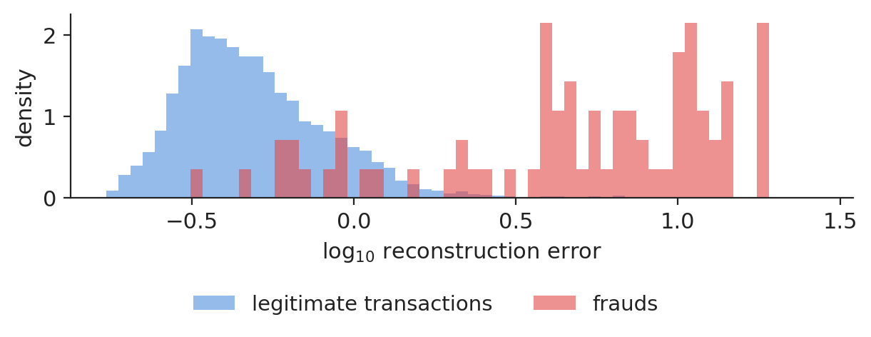
Reconstruction error of fraudulent and legitimate payments

Slide 11 in the PDF

On the test part the median reconstruction error of a fraud is 12.7 times that of a legitimate transaction. The two distributions still overlap: many frauds look normal to a model that only knows normal behaviour.

Chart: Reconstruction error of fraudulent and legitimate payments

Reconstruction error of the autoencoder on the test part, legitimate transactions (weighted) and frauds.

Source: ULB Machine Learning Group and Worldline, credit-card transactions (OpenML 1597). Data: own estimates; two days of September 2013; test = last 20 % of the time span.

Autoencoder without labels compared with a supervised classifier

Slide 12 in the PDF

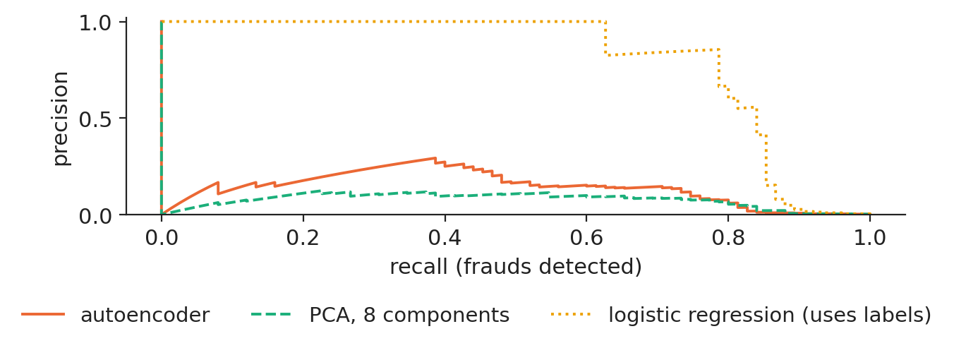
The PR-AUC on the test part is 14.2 % for the autoencoder (standard deviation 2.9 over 3 seeds), 7.6 % for PCA and 80.4 % for a logistic regression that uses the labels; a random score would give 0.131 %. The ROC-AUC is high for all three (94.4, 95.3 and 98.2 %): with one fraud in several hundred transactions it hides the differences that the PR-AUC shows.

Chart: Autoencoder without labels compared with a supervised classifier

Precision-recall curves on the test part, weighted to the full data.

Source: ULB Machine Learning Group and Worldline, credit-card transactions (OpenML 1597). Data: own estimates; two days of September 2013; test = last 20 % of the time span.

Bottleneck size and anomaly detection

Slide 13 in the PDF

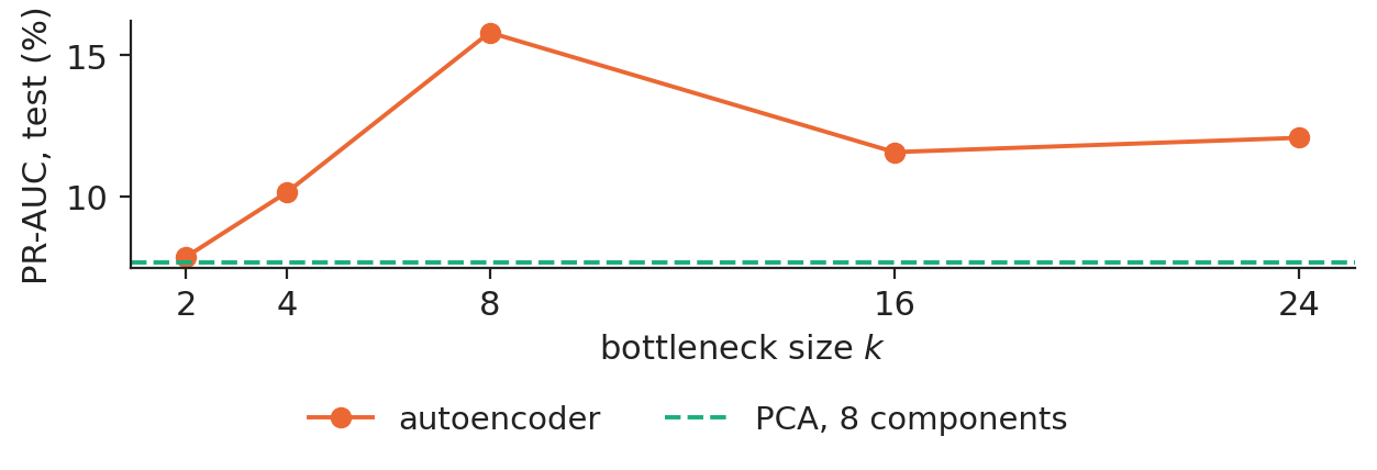
With a bottleneck of 2 the PR-AUC is 7.8 %, with 8 it is 15.8 % and with 24 it is 12.1 % (mean of 2 seeds); the best size is 8. Too narrow, and even normal payments are rebuilt badly; too wide, and the network learns to copy frauds as well.

Chart: Bottleneck size and anomaly detection

Test PR-AUC of the autoencoder by bottleneck size, with PCA as benchmark.

Source: ULB Machine Learning Group and Worldline, credit-card transactions (OpenML 1597). Data: own estimates; two days of September 2013; test = last 20 % of the time span.

In practice: choose \(k\) on a validation period, never on the frauds you will report on.

Frauds found among the top 0.1 % of scores

Slide 14 in the PDF

If the team reviews the 0.1 % highest scores of the test part, 57 alerts, it finds 8 frauds with the autoencoder (10.7 % of all test frauds), 0 with PCA and 48 with the logistic regression (64.0 %). Labels are worth a lot: supervised learning wins whenever confirmed frauds exist. The autoencoder is the detector of the unknown, a complement and not a replacement.

In practice: run both: the classifier for known fraud patterns, the autoencoder to surface new ones for investigators to label.

Section summary

An autoencoder is a model of normal behaviour; without labels it finds part of the frauds, with labels a supervised model finds far more.

Variational autoencoders

The VAE turns the autoencoder into a probabilistic generator by learning a distribution of codes.

The VAE makes the autoencoder a probabilistic generator

Slide 16 in the PDF

The encoder outputs a Gaussian \(q_\phi(\mathbf z\mid\mathbf x)=\mathcal N(\boldsymbol\mu_\phi(\mathbf x),\operatorname{diag}\boldsymbol\sigma_\phi^2(\mathbf x))\) and the decoder a likelihood \(p_\theta(\mathbf x\mid\mathbf z)\). The log-likelihood is bounded from below by the evidence lower bound (ELBO):

\[\log p_\theta(\mathbf x)\ge\mathbb E_{q_\phi(\mathbf z\mid\mathbf x)}\big[\log p_\theta(\mathbf x\mid\mathbf z)\big]-\mathrm{KL}\big(q_\phi(\mathbf z\mid\mathbf x)\,\|\,p(\mathbf z)\big).\]
(8.3)

The first term rewards good reconstructions; the second, the Kullback–Leibler divergence (KL) from the prior \(p(\mathbf z)=\mathcal N(0,I)\), packs all codes around the origin, so that a random code decodes to a realistic image. For Gaussians it has the closed form \(\tfrac12\sum_j(\mu_j^2+\sigma_j^2-\log\sigma_j^2-1)\).

The reparameterisation trick

Slide 17 in the PDF

Sampling \(\mathbf z\) is not differentiable, but \(\mathbf z=\boldsymbol\mu_\phi(\mathbf x)+\boldsymbol\sigma_\phi(\mathbf x)\odot\boldsymbol\varepsilon\) with \(\boldsymbol\varepsilon\sim\mathcal N(0,I)\) is: the randomness sits in \(\boldsymbol\varepsilon\), which does not depend on the parameters. Our VAE is trained on Fashion-MNIST, 60,000 training and 10,000 test grey images of 28 × 28 pixels showing 10 kinds of clothing, with a Bernoulli decoder; the network 784–400–200–\(k\) has 798,816 parameters for \(k=16\) and is trained for 20 epochs.

A two-dimensional latent space separates the product types

Slide 18 in the PDF

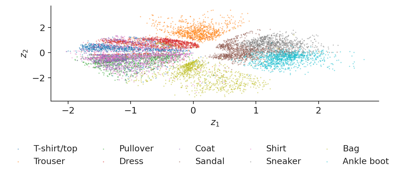
With only two latent dimensions and no labels, shoes, bags and garments fall into separate regions. A 15-nearest-neighbour classifier on the two latent means reaches 71.7 % accuracy (5-fold, test images): the VAE has learnt an organisation of the products without being told what they are.

Chart: A two-dimensional latent space separates the product types

Latent means of the 10,000 test images, VAE with \(k=2\), coloured by class.

Source: Fashion-MNIST, Zalando Research (Xiao et al., 2017). Data: own estimates; 60,000 training and 10,000 test images.

Quality of VAE reconstructions and generated samples

Slide 19 in the PDF

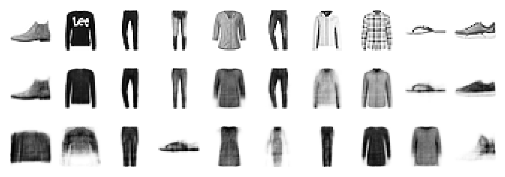
The first row shows real test images, the second their reconstructions through a 16-dimensional code, the third new images decoded from random codes. The blur comes from the Gaussian posterior and the pixel-wise loss: the decoder averages over the plausible details.

Chart: Quality of VAE reconstructions and generated samples

Real, reconstructed and generated images, VAE with \(k=16\).

Source: Fashion-MNIST, Zalando Research (Xiao et al., 2017). Data: own estimates; 60,000 training and 10,000 test images.

Trade-off between reconstruction and the KL penalty during training

Slide 20 in the PDF

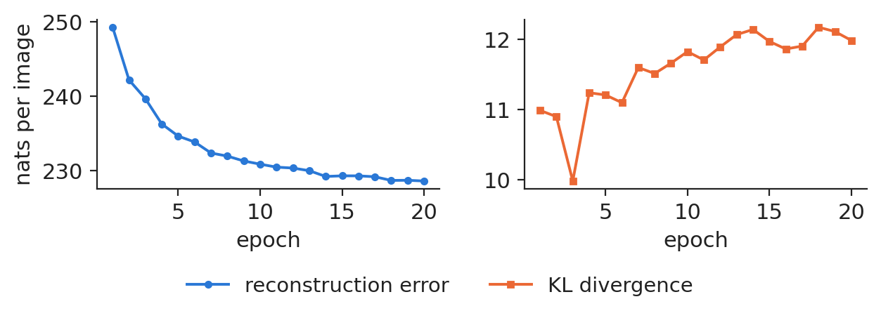
On the test images, after the last epoch, the reconstruction term is 228.6 nats per image and the KL term 12.0 nats, so the ELBO is −240.6 nats. The KL rises while the error falls: the encoder spends more information on each image as it learns.

Chart: Trade-off between reconstruction and the KL penalty during training

Reconstruction and KL terms of the ELBO on the test images, by epoch.

Source: Fashion-MNIST, Zalando Research (Xiao et al., 2017). Data: own estimates; 60,000 training and 10,000 test images.

β-VAE: reconstruction quality and latent-space structure

Slide 21 in the PDF

Multiplying the KL term by \(\beta\) changes the balance. With \(\beta=0.5\) the reconstruction term is 222.5 nats and 9 of the 16 latent dimensions are active (KL above 0.05); with \(\beta=4\) the reconstruction worsens to 242.5 nats and only 4 dimensions stay active. A larger \(\beta\) gives smoother and more disentangled codes; a smaller one gives better copies and poorer samples.

In practice: for scenario generation prefer a tidy latent space (\(\beta\ge1\)); for compression prefer reconstruction (\(\beta<1\)).

Section summary

The VAE maximises the ELBO = reconstruction − KL; the reparameterisation trick makes it trainable and β sets the balance.

Generative adversarial networks

A GAN learns to sample from the data distribution by playing against a discriminator.

Generative adversarial networks: generator and discriminator

Slide 23 in the PDF

The generator \(G\) turns noise \(\mathbf z\) into fake data; the discriminator \(D\) gives the probability that its input is real. They play

\[\min_G\max_D\ \mathbb E_{\mathbf x\sim p_{data}}[\log D(\mathbf x)]+\mathbb E_{\mathbf z}[\log(1-D(G(\mathbf z)))].\]
(8.4)

For a fixed generator the best discriminator is \(D^*(\mathbf x)=p_{data}(\mathbf x)/(p_{data}(\mathbf x)+p_G(\mathbf x))\), and the value of the game becomes \(-\log 4+2\,\mathrm{JS}(p_{data}\|p_G)\), where the Jensen–Shannon divergence (JS) is zero only when the generator reproduces the data. At that point \(D^*=1/2\) everywhere. A GAN never writes down a likelihood; it is judged by what its samples get right.

Training a GAN: alternate steps and the non-saturating loss

Slide 24 in the PDF

Each step first updates the discriminator on a batch of 256 real and 256 fake days, then the generator on fresh noise. The generator minimises \(-\log D(G(\mathbf z))\) instead of \(\log(1-D(G(\mathbf z)))\), whose gradient vanishes when the discriminator wins early. Our GAN learns the standardised daily log returns of the S&P 500 from 4 Jan 2005 to the end of 2019, 3,774 days; the generator has 4,801 and the discriminator 4,353 parameters, trained for 6,000 steps with 3 seeds.

The two losses settle near the equilibrium values

Slide 25 in the PDF

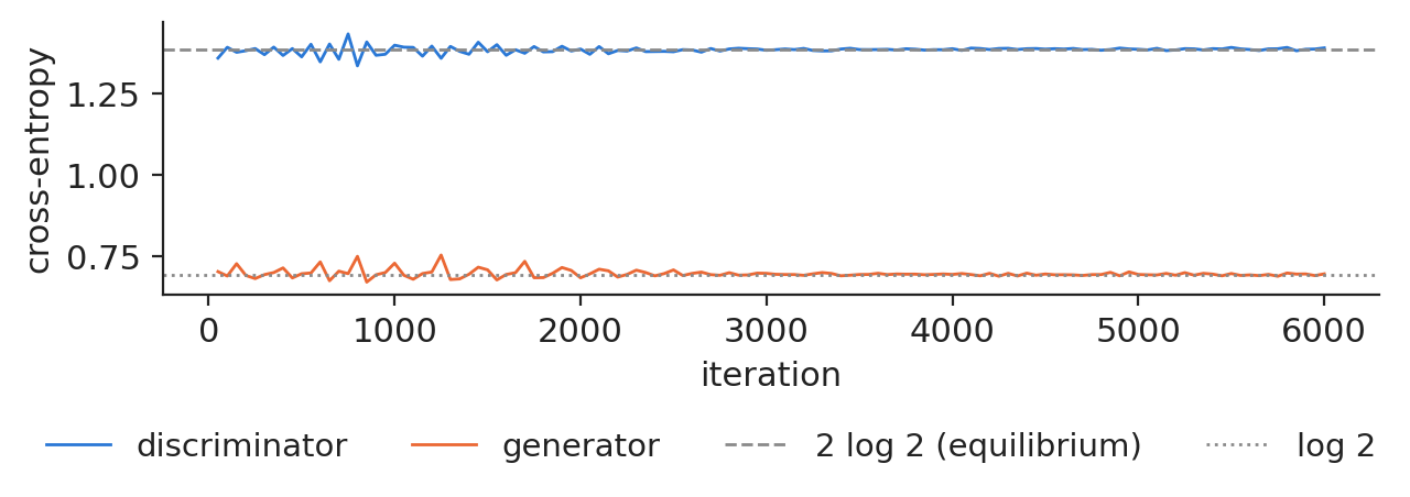
The discriminator loss hovers around \(2\log 2\) and the generator loss around \(\log 2\), the values that correspond to \(D^*=1/2\). There is no proof of convergence for gradient play, and the curves do not measure sample quality: they only show that neither player has won.

Chart: The two losses settle near the equilibrium values

Discriminator and generator losses during training, seed 1.

Source: Yahoo Finance, daily quotes. Data: own estimates; S&P 500 4 Jan 2005 to 31 Dec 2019, trading days.

The GAN reproduces the fat tails missed by the Gaussian model

Slide 26 in the PDF

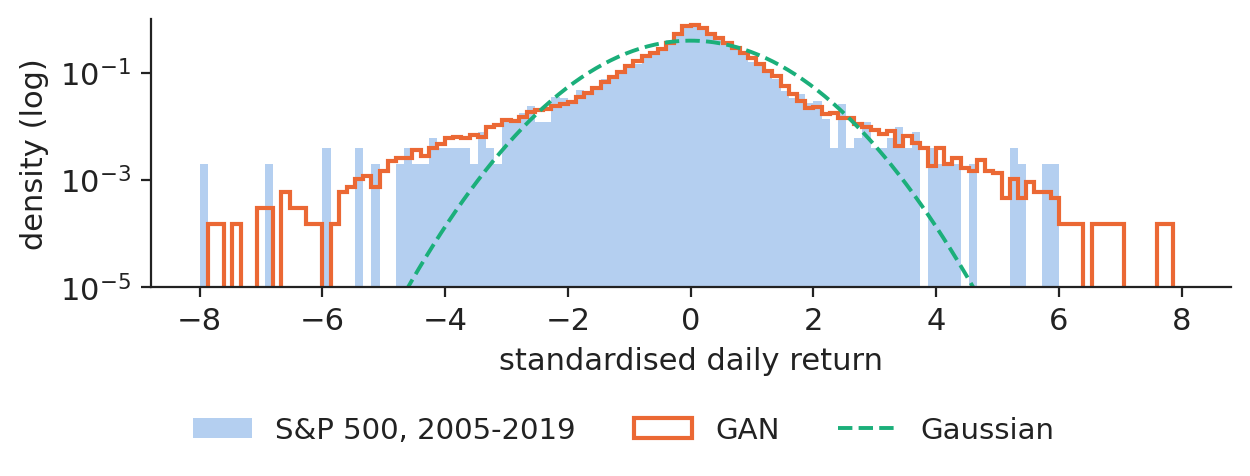
The excess kurtosis of the real returns is 11.86; the GAN samples reach 6.65 (standard deviation 0.48 over 3 seeds), against 0 for the Gaussian. The Kolmogorov–Smirnov distance to the real returns is 0.030 for the GAN and 0.115 for the fitted Gaussian.

Chart: The GAN reproduces the fat tails missed by the Gaussian model

Density, on a log scale, of real standardised returns, GAN samples and the Gaussian.

Source: Yahoo Finance, daily quotes. Data: own estimates; S&P 500 4 Jan 2005 to 31 Dec 2019, trading days.

A risk check: 1 % Value-at-Risk on the years after training

Slide 27 in the PDF

The 1 % quantile of daily returns fitted on 2005–2019 is −3.48 % by historical simulation, −3.61 % from the GAN samples and −2.67 % for the Gaussian. On the 1,717 days from 2 Jan 2020 to 30 Oct 2026, a correct 1 % VaR is exceeded on about 17 days. The exceedance rates are 1.11 % (historical), 0.95 % (GAN) and 2.39 % (Gaussian). The expected shortfall (ES), the mean loss beyond the VaR, depends on the same tail. These are unconditional quantiles: none of the three reacts to volatility.

In practice: a generator is only as good as the risk number it reproduces: backtest it like any VaR model.

A GAN on single days cannot learn volatility clustering

Slide 28 in the PDF

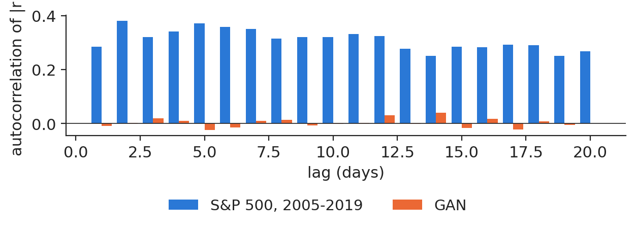
The autocorrelation of absolute real returns is 0.28 at lag 1 and still 0.27 at lag 20: calm and turbulent periods cluster. The GAN draws days independently, so its autocorrelation is −0.01: the right marginal distribution with the wrong dynamics. Sequence generators, such as TimeGAN or Quant GANs, generate whole paths for this reason.

Chart: A GAN on single days cannot learn volatility clustering

Autocorrelation of absolute returns, lags 1 to 20, real returns and GAN samples.

Source: Yahoo Finance, daily quotes. Data: own estimates; S&P 500 4 Jan 2005 to 31 Dec 2019, trading days.

Mode collapse and the Wasserstein GAN

Slide 29 in the PDF

A generator can win by producing only a few convincing samples, for example only calm days and never a crash: mode collapse. The Wasserstein GAN (WGAN) replaces the Jensen–Shannon divergence by the Wasserstein distance \(W_1(p_{data},p_G)=\sup_{\|f\|_L\le1}\mathbb E_{p_{data}}[f]-\mathbb E_{p_G}[f]\), computed by a 1-Lipschitz critic, which gives useful gradients even when the two distributions do not overlap.

In practice: a stress-test generator that has collapsed onto calm days is worse than no generator.

Section summary

A GAN reproduces the fat tails of returns and a usable 1 % VaR, but not volatility clustering when it is trained on single days.

Diffusion models

A diffusion model learns to undo, step by step, a process that turns data into noise.

Diffusion models: forward noising and reverse denoising

Slide 31 in the PDF

The forward process adds a little Gaussian noise at each of \(T\) = 200 steps, \(q(\mathbf x_t\mid\mathbf x_{t-1})=\mathcal N(\sqrt{1-\beta_t}\,\mathbf x_{t-1},\beta_tI)\), with \(\beta_t\) rising linearly from \(10^{-4}\) to 0.02. Any step can be reached in one draw,

\[\mathbf x_t=\sqrt{\bar\alpha_t}\,\mathbf x_0+\sqrt{1-\bar\alpha_t}\,\boldsymbol\varepsilon,\qquad \bar\alpha_t=\prod_{s=1}^t(1-\beta_s),\]
(8.5)

and at the last step \(\mathbf x_T\) is almost standard normal. The forward process has no parameters: only the reverse is learnt.

The forward process on a real yield curve

Slide 32 in the PDF

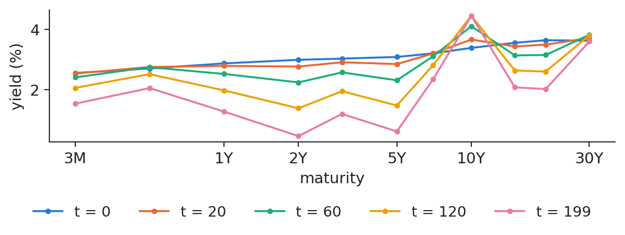
The chart applies (8.5) to the euro-area AAA curve of 30 Oct 2026, 11 maturities from 3 months to 30 years. By step 199 the shape is gone and only noise remains; the network must learn to walk back, one small step at a time.

Chart: The forward process on a real yield curve

The curve at noise steps 0, 20, 60, 120 and 199 (one draw of the noise).

Source: European Central Bank, euro area AAA yield curve. Data: curve of 30 Oct 2026; noise schedule of the lecture (mechanism).

Learning to denoise: predict the noise that was added

Slide 33 in the PDF

A network \(\boldsymbol\varepsilon_\theta(\mathbf x_t,t)\) sees a noisy curve and the step, and predicts the noise:

\[\mathcal L(\theta)=\mathbb E_{t,\mathbf x_0,\boldsymbol\varepsilon}\big\|\boldsymbol\varepsilon-\boldsymbol\varepsilon_\theta(\sqrt{\bar\alpha_t}\mathbf x_0+\sqrt{1-\bar\alpha_t}\boldsymbol\varepsilon,t)\big\|^2,\]
(8.6)

a simplified, reweighted ELBO. Generation starts from pure noise and applies \(\mathbf x_{t-1}=\big(\mathbf x_t-\beta_t\boldsymbol\varepsilon_\theta/\sqrt{1-\bar\alpha_t}\big)/\sqrt{\alpha_t}+\sqrt{\beta_t}\mathbf u\) down to \(t=0\). Our denoiser is an MLP with three hidden layers of 256 units and a sinusoidal embedding of \(t\), 145,675 parameters, trained for 12,000 steps on the 5,664 daily curves of the European Central Bank from 6 Sep 2004 to 30 Oct 2026.

The two regimes of euro rates in diffusion and Gaussian samples

Slide 34 in the PDF

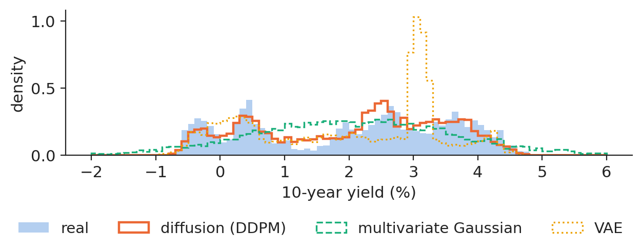
The real 10-year yield ranges from −0.82 % to 4.78 % and is negative on 13.8 % of the days: there is a low-rate and a normal-rate regime. The Wasserstein distance between the generated and the real 10-year yield is 0.149 percentage points for the diffusion model, 0.191 for a two-factor VAE and 0.325 for a multivariate Gaussian.

Chart: The two regimes of euro rates in diffusion and Gaussian samples

Density of the 10-year yield, real curves and 5,000 curves from each generator.

Source: European Central Bank, euro area AAA yield curve. Data: own estimates; 6 Sep 2004 to 30 Oct 2026, business days.

Diffusion preserves the nonlinear co-movement of level and slope

Slide 35 in the PDF

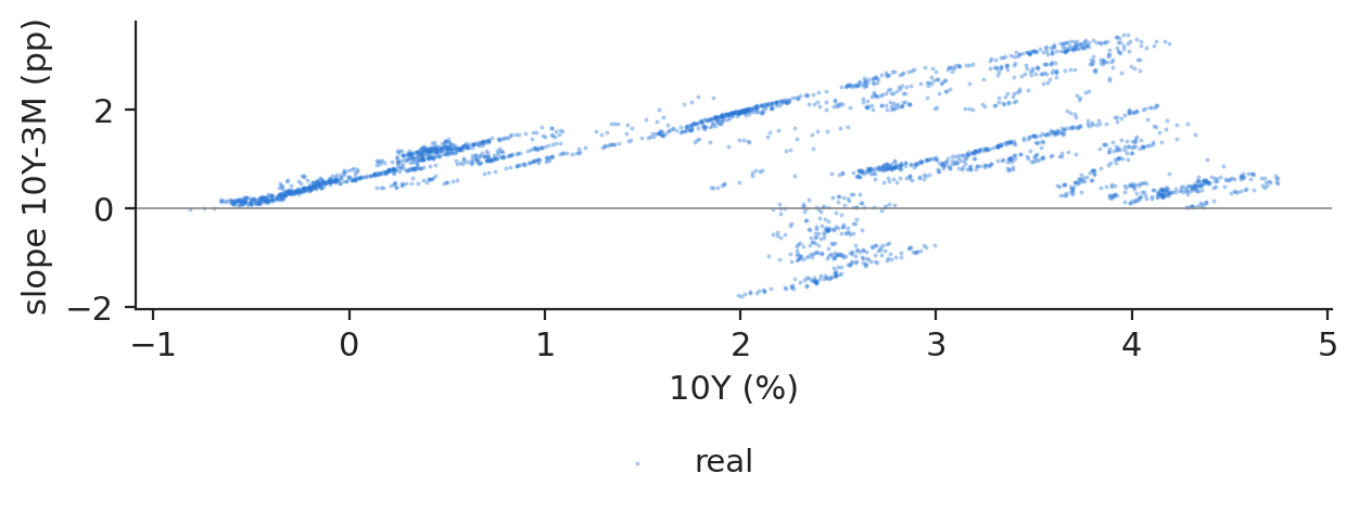
A curve is inverted when the 10-year yield is below the 3-month yield. This happened on 8.7 % of the real days; 10.2 % of the diffusion samples and 14.7 % of the Gaussian samples are inverted. The Wasserstein distance of the slope is 0.099 for the diffusion model, 0.242 for the VAE and 0.113 for the Gaussian.

Chart: Diffusion preserves the nonlinear co-movement of level and slope

Level (10-year yield) against slope (10 years minus 3 months): real curves, diffusion samples and Gaussian samples.

Source: European Central Bank, euro area AAA yield curve. Data: own estimates; 6 Sep 2004 to 30 Oct 2026, business days.

A two-factor VAE of the curve rediscovers level and slope

Slide 36 in the PDF

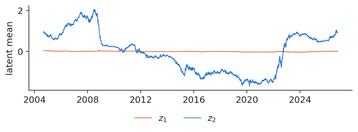
The VAE used as a benchmark compresses each curve into two latent numbers. Their correlations with the level (mean of the 11 yields) and the slope reach 0.99 and 0.66 in absolute value: without being told, the latent path tracks the low-rate era of 2014–2021 and the tightening of 2022.

Chart: A two-factor VAE of the curve rediscovers level and slope

Latent means of the two-factor VAE over time.

Source: European Central Bank, euro area AAA yield curve. Data: own estimates; 6 Sep 2004 to 30 Oct 2026, business days.

Section summary

Diffusion learns to undo noise; on euro yield curves it keeps both rate regimes and the inversions that a Gaussian misses.

Generative models in practice

Synthetic data are useful only after they pass the same checks as real data.

Evaluation criteria for synthetic financial data

Slide 38 in the PDF

Four questions. Fidelity: do the marginals, the tails and the dependence across assets and over time match? Diversity: are extreme days and regimes present in the right proportions, with no mode collapse? Utility: does a model trained on synthetic data and tested on real data (TSTR) work? Privacy: is any sample too close to a real record? On our data the GAN gets the tails right and the clustering wrong; the diffusion model gets the regimes and the inversions right, the Gaussian does not.

In practice: never use synthetic data for a decision before it passes the same backtests as the model it feeds.

Choosing a generative model

Slide 39 in the PDF

Autoencoders are the tool to monitor (an anomaly score), VAEs to compress and explore (smooth latent factors), diffusion models to simulate faithfully at the cost of 200 network passes per sample, and GANs when sampling must be fast and the training can be watched closely.

Section summary

Pick the family by the use: monitoring, compression, faithful simulation or fast sampling; then backtest the output.

Videos: the intuition behind the mathematics (in English)

Abbreviations

AEautoencoder
ASEBucharest University of Economic Studies
DDPMdenoising diffusion probabilistic model
ELBOevidence lower bound
ESexpected shortfall
GANgenerative adversarial network
IPEInstitute for Economic Forecasting, Romanian Academy
JSJensen–Shannon divergence
KLKullback–Leibler divergence
LLMlarge language model
MLPmultilayer perceptron
MNISTModified National Institute of Standards and Technology handwritten digits
PCAprincipal component analysis
PR-AUCarea under the precision-recall curve
ReLUrectified linear unit
ROCreceiver operating characteristic
ROC-AUCarea under the ROC curve
TSTRtrain on synthetic, test on real
VAEvariational autoencoder
VaRValue-at-Risk
WGANWasserstein GAN

References

  • Arjovsky, M., Chintala, S. & Bottou, L. (2017). Wasserstein generative adversarial networks. Proceedings of ICML, PMLR 70, 214–223. arXiv:1701.07875
  • Bishop, C. M. & Bishop, H. (2024). Deep Learning: Foundations and Concepts, ch. 16–20. Springer. doi:10.1007/978-3-031-45468-4
  • Cont, R. (2001). Empirical properties of asset returns: stylized facts and statistical issues. Quantitative Finance, 1(2), 223–236. doi:10.1080/713665670
  • Dal Pozzolo, A., Caelen, O., Johnson, R. A. & Bontempi, G. (2015). Calibrating probability with undersampling for unbalanced classification. IEEE Symposium Series on Computational Intelligence, 159–166. doi:10.1109/SSCI.2015.33
  • Goodfellow, I., Pouget-Abadie, J., Mirza, M., Xu, B., Warde-Farley, D., Ozair, S., Courville, A. & Bengio, Y. (2014). Generative adversarial nets. Advances in Neural Information Processing Systems, 27. arXiv:1406.2661
  • Higgins, I., Matthey, L., Pal, A. et al. (2017). beta-VAE: Learning basic visual concepts with a constrained variational framework. International Conference on Learning Representations. openreview.net
  • Ho, J., Jain, A. & Abbeel, P. (2020). Denoising diffusion probabilistic models. Advances in Neural Information Processing Systems, 33. arXiv:2006.11239
  • Jheng, S.-L., Tak, R., Găman, Ș., Mazurencu-Marinescu-Pele, M. & Pele, D. T. (2026). Can foundation models manage risk? Zero-shot VaR and ES forecasting with conformal calibration in CEE markets. Economic Computation and Economic Cybernetics Studies and Research, 60(2), 267–290. doi:10.24818/18423264/60.2.26.14
  • Kingma, D. P. & Welling, M. (2014). Auto-encoding variational Bayes. International Conference on Learning Representations. arXiv:1312.6114
  • Kupiec, P. H. (1995). Techniques for verifying the accuracy of risk measurement models. Journal of Derivatives, 3(2), 73–84. doi:10.3905/jod.1995.407942
  • Pele, D. T., Bolovăneanu, V., Lin, M.-B., Ren, R., Ginavar, A. T., Spilak, B., Andrei, A.-V., Toma, F.-M., Lessmann, S. & Härdle, W. K. (2026). In the beginning was the word: LLM-VaR and LLM-ES. SSRN Working Paper 5104383. doi:10.2139/ssrn.5104383
  • Sohl-Dickstein, J., Weiss, E., Maheswaranathan, N. & Ganguli, S. (2015). Deep unsupervised learning using nonequilibrium thermodynamics. Proceedings of ICML, PMLR 37, 2256–2265. arXiv:1503.03585
  • Svensson, L. E. O. (1994). Estimating and interpreting forward interest rates: Sweden 1992–1994. NBER Working Paper 4871. doi:10.3386/w4871
  • Wiese, M., Knobloch, R., Korn, R. & Kretschmer, P. (2020). Quant GANs: Deep generation of financial time series. Quantitative Finance, 20(9), 1419–1440. doi:10.1080/14697688.2020.1730426
  • Xiao, H., Rasul, K. & Vollgraf, R. (2017). Fashion-MNIST: A novel image dataset for benchmarking machine learning algorithms. arXiv:1708.07747
  • Yoon, J., Jarrett, D. & van der Schaar, M. (2019). Time-series generative adversarial networks. Advances in Neural Information Processing Systems, 32. papers.nips.cc/paper/8789

Text written for the web version of the lecture; numbers, charts and sources come from the slides and their Quantlets.