

Statistics of Financial Markets

Chapter 1 · Data, Returns and Indicators

The slide of the lecture is on the left, the same figure or table on the right, computed in the browser from the same data. The ▶ button moves the parameter step by step; the tables and worked examples are recomputed with it.

Financial Data: Sources and Quality · From Prices to Returns · Simple and Log Returns · Multi-Period and Portfolio Returns · Annualisation · Descriptive Statistics of Returns · Performance Indicators

Financial Data: Sources and Quality

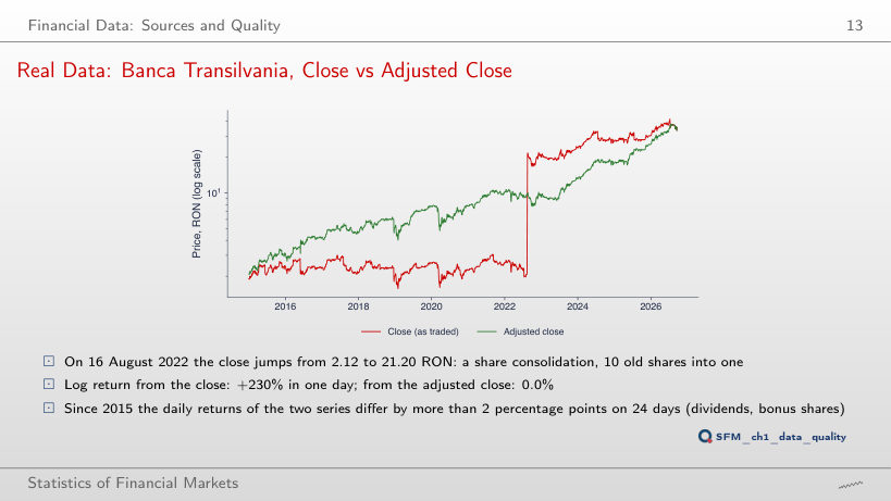
Real Data: Banca Transilvania, Close vs Adjusted Close
Slide 13: Real Data: Banca Transilvania, Close vs Adjusted Close
Slide 13
    Question for the room On the slide, the daily returns of the two series differ by more than 2 percentage points on 24 days since 2015. The ▶ button raises the threshold. How many days remain at a threshold of 10 percentage points?
    Answer

    11 days. Besides the consolidation of 16 August 2022 (+230.3% from the close, 0.0% from the adjusted close), 10 other days show a gap of more than 10 percentage points between the two log returns, all with the close falling; the largest, 19.5 percentage points, on 3 August 2017. Above 20 percentage points only the consolidation remains. A return computed from the close would treat these days as losses of the shareholders, although the value of the holding did not change.

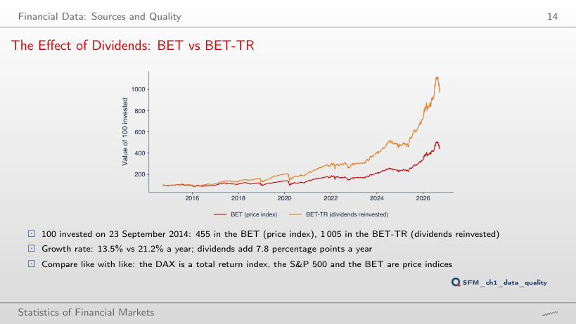
    The Effect of Dividends: BET vs BET-TR
    Slide 14: The Effect of Dividends: BET vs BET-TR
    Slide 14
      Question for the room The ▶ button moves the date of the investment from 2014 to 2025. With the investment made at the start of 2022, by how many percentage points a year does BET-TR grow faster than BET?
      Answer

      By 8.3 percentage points: 29.9% a year against 21.6%. The final values are 342 and 251, a gap of 91 units, much smaller than 1,005 against 455 for the investment of 23 September 2014. The gap between the growth rates, however, stays between 7.5 and 8.4 percentage points for every start year: dividends add roughly the same return every year, and their effect on wealth accumulates over time.

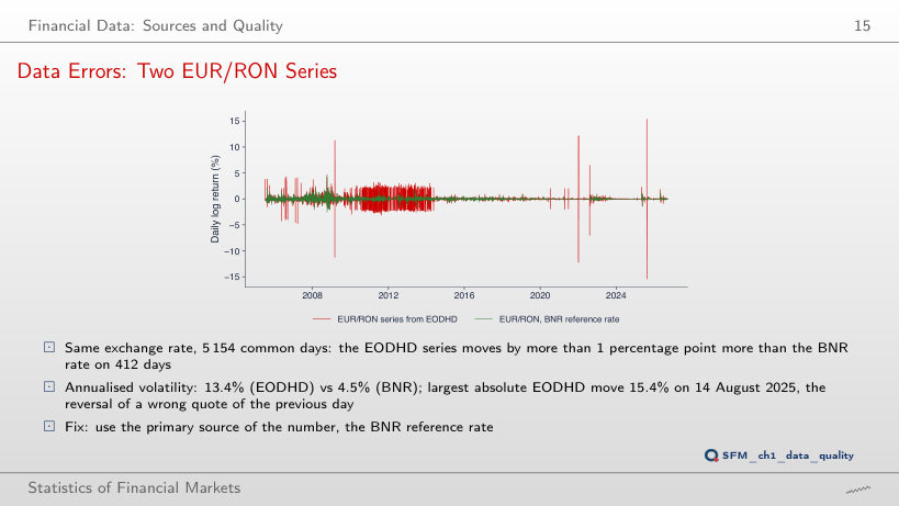
      Data Errors: Two EUR/RON Series
      Slide 15: Data Errors: Two EUR/RON Series
      Slide 15
        Question for the room The annualised volatility of the EODHD series is 13.4%, that of the BNR rate 4.5%. What does the volatility of the EODHD series become if we drop the 412 days on which the daily changes differ by more than 1 percentage point, that is 8% of the days?
        Answer

        About 4.7%, close to 4.3%, the volatility of the BNR rate on the same days. Volatility depends on squared deviations, so a few hundred wrong quotes triple it. Of the 412 days, 307 fall in 2010–2013. 283 days differ by more than 2 percentage points, 10 days by more than 5 percentage points.

        From Prices to Returns

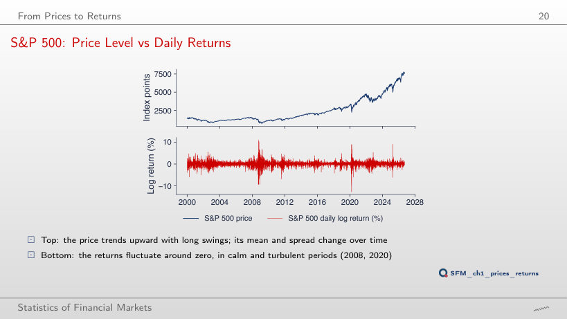
        S&P 500: Price Level vs Daily Returns
        Slide 20: S&P 500: Price Level vs Daily Returns
        Slide 20
          Question for the room The ▶ button splits the 2000–2026 sample into up to 6 equal subperiods. With 5 subperiods, what happens to the mean and the standard deviation of daily returns from one subperiod to the next?
          Answer

          The mean of returns stays close to zero, between −0.016% and 0.057% a day, while the mean of the price rises from 1,145 to 5,235 points. The standard deviation of returns, however, varies between 0.97% and 1.53% a day: returns fluctuate around a stable level, but their volatility changes over time. The ADF test rejects the unit root for returns (statistic −14.3), not for the log price (statistic −2.08, p-value 0.56).

          Simple and Log Returns

          Simple vs Log Returns on Real Extremes
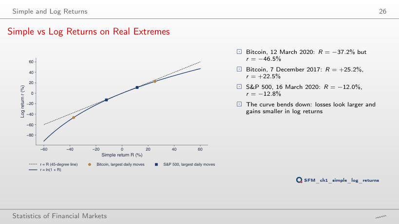
          Slide 26: Simple vs Log Returns on Real Extremes
          Slide 26

          Worked example: simple and log return of a real price pair

          \[r_t = \ln\frac{P_t}{P_{t-1}} = \ln(1+R_t) = R_t - \frac{R_t^2}{2} + \frac{R_t^3}{3} - \dots\]
              Question for the room Bitcoin, 7 December 2017: R = +25.2%, r = +22.5%, so R − r = 2.7 percentage points. What is the gap R − r for a fall of the same size, R = −25.2%?
              Answer

              3.8 percentage points: r = ln(0.748) = −29.0%. The function ln is concave, and the gap is larger for falls than for rises of the same size. The approximation R²/2 = 3.2 percentage points is the same for both signs; the R³/3 term of the Taylor series corrects it upwards for falls and downwards for rises. At R = −37.2% (Bitcoin, 12 March 2020), the gap reaches 9.3 percentage points.

              Multi-Period and Portfolio Returns

              Growth of 100 Invested, 2015–2026
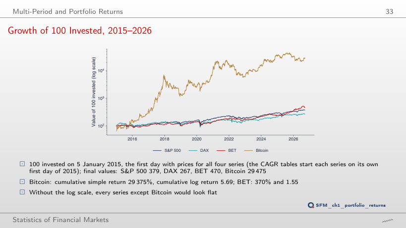
              Slide 33: Growth of 100 Invested, 2015–2026
              Slide 33

              Worked example: compounding over many periods

              \[W_T = W_0\prod_{t=1}^{T}(1+R_t) = W_0\exp\Big(\sum_{t=1}^{T} r_t\Big), \qquad \text{CAGR} = \Big(\frac{P_T}{P_0}\Big)^{1/Y} - 1\]
                  Question for the room The ▶ button moves the date of the investment from 2015 to 2025. With the investment made at the start of 2022, which of the four series has the largest final value?
                  Answer

                  BET: 251, against Bitcoin 170, S&P 500 161 and DAX 159. For the investment of 2015, Bitcoin reaches 29,475, and for that of 2018 592, still first. The ranking by cumulative return depends on the start date.

                  Real Data: a TLV–SNP Portfolio
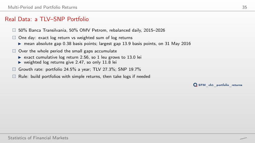
                  Slide 35: Real Data: a TLV–SNP Portfolio
                  Slide 35

                  Cumulative returns and annual growth, 2015–2026

                  Worked example: the portfolio return on the day with the largest gap

                  \[R_{p,t} = w\,R_{1,t} + (1-w)\,R_{2,t}, \qquad r_{p,t} = \ln(1+R_{p,t}) \neq w\,r_{1,t} + (1-w)\,r_{2,t}\]
                      Question for the room With equal weights, the weighted sum of log returns gives a cumulative log return of 2.47 instead of 2.56. The ▶ button moves the TLV weight from 10% to 90%. At which weight is the gap between the two cumulative returns largest?
                      Answer

                      At 50%: 0.093. At 25% and 75% the gap is about 0.07, at 10% and 90% only 0.033. The daily gap is about w(1 − w)(RTLV − RSNP)²/2, largest for equal weights and zero for a single stock. The largest daily gap, 13.9 basis points on 31 May 2016, covers three trading days: SNP has no prices on 27 and 30 May 2016, so both returns run from 26 May; TLV rises by 6.6%, SNP falls by 4.0%.

                      Annualisation

                      Annualising the Mean and the Volatility
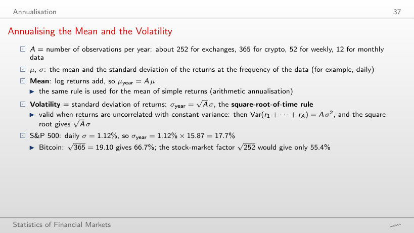
                      Slide 37: Annualising the Mean and the Volatility
                      Slide 37

                      Annualised volatility (%) by frequency of the log returns

                      Worked example: annualising the mean and the volatility

                      \[\mu_{\text{year}} = A\,\mu, \qquad \sigma_{\text{year}} = \sqrt{A}\,\sigma, \qquad A = n/Y\]
                          Question for the room From daily returns, the annualised volatility of the S&P 500 over 2015–2026 is 17.7%. The ▶ button switches to weekly and monthly returns. What does √12 × σ computed from the monthly returns give?
                          Answer

                          15.0%; from weekly returns, 16.7%. The square-root-of-time rule assumes uncorrelated returns with constant variance, and the S&P 500 does not follow it exactly over 2015–2026. The monthly series has only 140 returns, so its estimate also has a larger error. For Bitcoin the three values are close: 66.7%, 66.7% and 66.3%.

                          Precision of the Estimated Mean
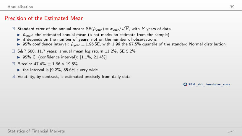
                          Slide 39: Precision of the Estimated Mean
                          Slide 39

                          Annual mean of the daily log returns and its precision

                          Worked example: the standard error of the annual mean

                          \[\text{SE}(\hat\mu_{\text{year}}) = \frac{\sigma_{\text{year}}}{\sqrt{Y}}, \qquad \hat\mu_{\text{year}} \pm z\,\text{SE}\]
                              Question for the room Over 2015–2026 (11.7 years), the 95% confidence interval of the annual mean of the S&P 500 is [1.1%; 21.4%]. The ▶ button moves the start of the sample. With the start in 2020 (6.7 years), does the interval contain 0?
                              Answer

                              Yes: 12.7% ± 15.3%, that is [−2.6%; 28.1%]. The estimated mean is higher than over 2015–2026, but the standard error rises from 5.2% to 7.8%, roughly as 1/√Y. The 1,686 daily returns do not help: the precision of the mean depends on the number of years. An interval that contains 0 does not show that the mean is zero, only that 6.7 years of data do not separate it from noise.

                              Descriptive Statistics of Returns

                              Daily Log Returns: Indices and Bitcoin, 2015–2026
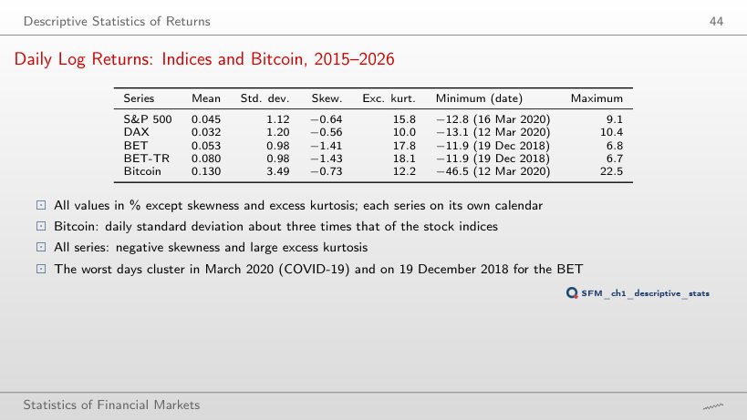
                              Slide 44: Daily Log Returns: Indices and Bitcoin, 2015–2026
                              Slide 44

                              Log returns (%), each series on its own calendar

                                Question for the room For daily returns, the excess kurtosis of the S&P 500 is 15.8. The ▶ button switches to weekly and monthly returns. What happens to the excess kurtosis?
                                Answer

                                It falls: 7.2 for weekly and 0.7 for monthly returns. A monthly return is the sum of about 21 daily returns, and the sum is closer to the Normal distribution than each term. For Bitcoin the excess kurtosis falls from 12.2 to 2.1 and 0.2. The skewness of the S&P 500 stays negative at all three frequencies (−0.64, −0.89, −0.50).

                                Daily Log Returns: Five BVB Stocks, 2015–2026
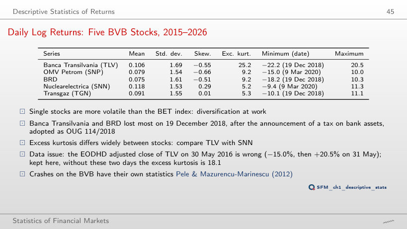
                                Slide 45: Daily Log Returns: Five BVB Stocks, 2015–2026
                                Slide 45

                                Log returns (%), adjusted prices

                                  Question for the room Banca Transilvania has an excess kurtosis of 25.2, the largest in the table. The ▶ button removes the returns of 30 and 31 May 2016. What does the excess kurtosis of TLV become?
                                  Answer

                                  18.1. The adjusted close of 30 May 2016 does not fit those of the neighbouring days, so the daily returns are −15.0% and +20.5%, although over the two days together the adjusted close rises by 5.5%. The two days raise the excess kurtosis from 18.1 to 25.2 and give the maximum of the table; without them, the largest daily return of TLV is 11.2%, and the skewness becomes −1.08. TLV remains the stock with the largest kurtosis. Two days out of 2,677 change the fourth moment, which depends on the fourth power of the deviations.

                                  Histograms vs the Normal Distribution
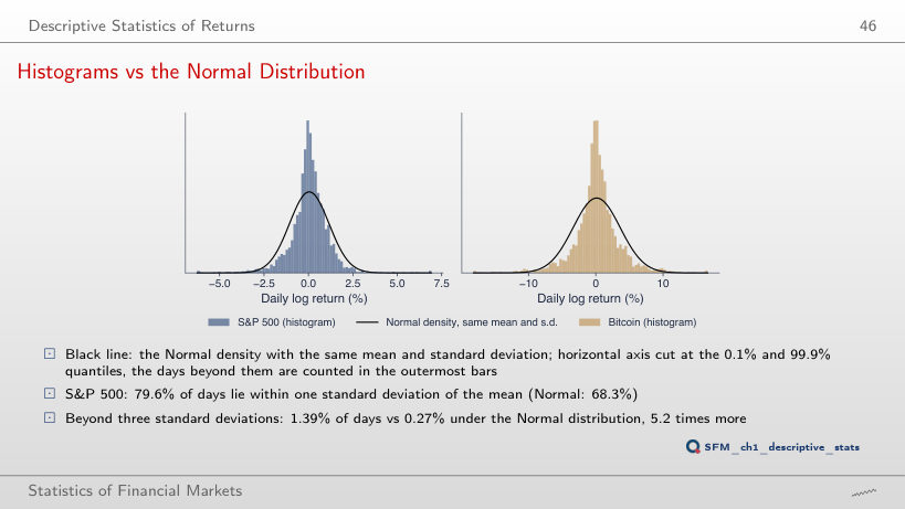
                                  Slide 46: Histograms vs the Normal Distribution
                                  Slide 46
                                    Question for the room Beyond 3 standard deviations, the S&P 500 has 5.2 times as many days as the Normal distribution. The ▶ button raises the threshold. How many times as many days does the S&P 500 have beyond 4 standard deviations?
                                    Answer

                                    About 113 times: 21 days out of 2,943 (0.71%), against 0.0063% for the Normal distribution. The ratio grows with the threshold, because the tail of the Normal distribution falls very fast; for Bitcoin the ratio is 103 (28 days). The frequency of extreme days does not follow from the standard deviation through the Normal distribution.

                                    Time-Varying Volatility
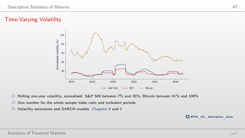
                                    Slide 47: Time-Varying Volatility
                                    Slide 47
                                      Question for the room With a 250-day window, the annualised volatility of the S&P 500 reaches at most 35.0%. The ▶ button changes the window. What is the maximum with a 21-day window (one month)?
                                      Answer

                                      97.5%, in the window ending on 6 April 2020. A short window follows a turbulent period such as March 2020 quickly; a one-year window dilutes it with the calm months before and after. The minimum falls too, from 6.7% to 3.5%. A short window reacts fast, but its estimate has a larger error.

                                      Performance Indicators

                                      Sharpe Ratios with 95% Intervals, 2015–2026
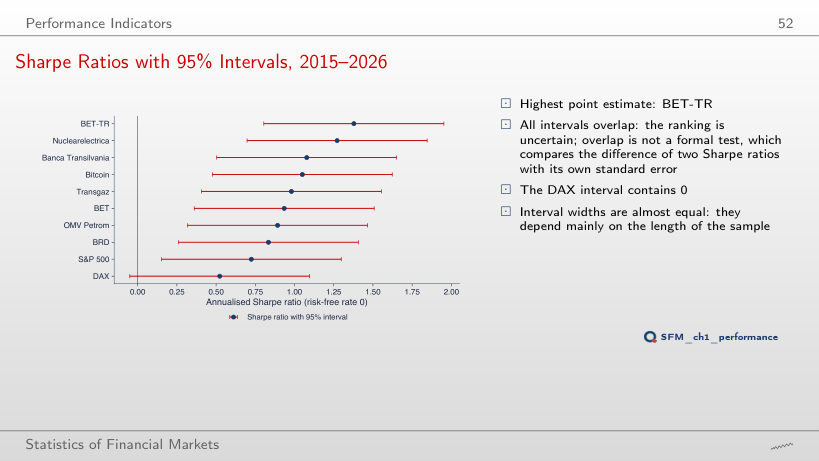
                                      Slide 52: Sharpe Ratios with 95% Intervals, 2015–2026
                                      Slide 52
                                        Question for the room Over 2015–2026 (11.7 years), the 95% confidence interval is the Sharpe ratio ± 0.57. The ▶ button moves the start of the sample towards 2024. With the start in 2023 (3.7 years), what does the half-width of the interval become?
                                        Answer

                                        About ± 1.02, roughly 1.96/√3.7. The standard error of the annual Sharpe ratio falls as 1/√Y, with Y the number of years, however many daily observations the sample holds. With the start in 2023, the Nuclearelectrica interval contains 0, and the DAX interval no longer does.

                                        Drawdowns over the Full History
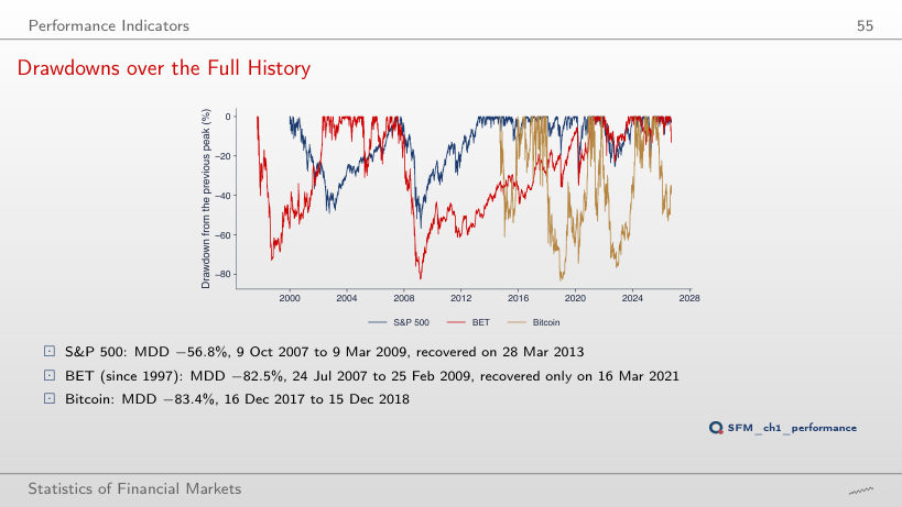
                                        Slide 55: Drawdowns over the Full History
                                        Slide 55

                                        Worked example: the maximum drawdown of a real price path

                                        \[\text{DD}_t = \frac{P_t}{\max_{s \le t} P_s} - 1, \qquad \text{MDD} = \min_t \text{DD}_t, \qquad g = \frac{x}{1-x},\ x = |\text{MDD}|\]
                                            Question for the room More than 20% below the peak lie 27% of the S&P 500 days, 56% of the BET days and 66% of the Bitcoin days. The ▶ button raises the threshold. What share of its days did BET, since 1997, spend more than 50% below the previous peak?
                                            Answer

                                            18%, almost one day in five; the S&P 500 only 0.3%, Bitcoin 31.6%. A fall of 50% needs a gain of 100% to recover. The depth of the maximum drawdown (−82.5% for BET) does not say how long the fall lasts; the share of days below the threshold shows the duration.

                                            Volatility Drag on Real Data
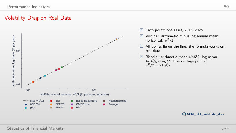
                                            Slide 59: Volatility Drag on Real Data
                                            Slide 59

                                            Worked example: arithmetic minus log mean, 2015–2026

                                            \[\mu_{\text{log}} \approx \mu_{\text{arith}} - \frac{\sigma^2}{2}, \qquad \text{CAGR} = e^{\mu_{\text{log}}} - 1\]
                                                Question for the room Arithmetic mean 10% a year, σ = 30%: the volatility drag is 4.5%, and 1 RON becomes 1.73 RON after 10 years. The ▶ button raises σ. With σ = 60%, does wealth grow over 10 years?
                                                Answer

                                                No. The drag is σ²/2 = 18%, four times larger, and the growth rate is 10% − 18% = −8% a year: after 10 years 1 RON becomes 0.45 RON. A positive arithmetic mean does not guarantee that wealth grows. On real data, the drag of Bitcoin is 22.1 percentage points, close to σ²/2 = 21.9%.

                                                Performance Indicators: Indices and Bitcoin, 2015–2026
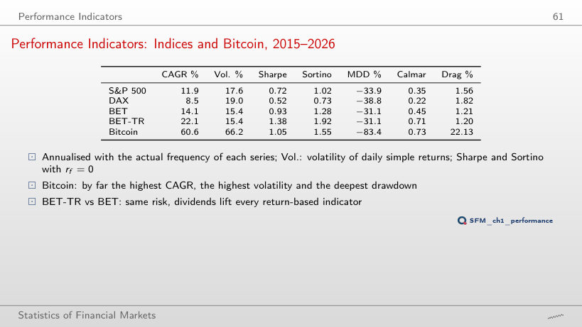
                                                Slide 61: Performance Indicators: Indices and Bitcoin, 2015–2026
                                                Slide 61

                                                Performance indicators; Sharpe with its standard error in brackets

                                                Worked example: the Sharpe ratio and its standard error

                                                \[\text{SR} = \frac{\mu - r_f}{\sigma}\sqrt{A}, \qquad \text{SE}(\widehat{\text{SR}}) \approx \sqrt{\frac{1 + \text{SR}_d^2/2}{n}}\,\sqrt{A}\]
                                                    Question for the room With rf = 0, the Sharpe ratio of the S&P 500 is 0.72. The ▶ button raises the risk-free rate up to 5% a year. What does the Sharpe ratio of the S&P 500 become at rf = 5%?
                                                    Answer

                                                    0.44: it falls by rf/σ = 5%/17.6% = 0.28. For Bitcoin it falls only from 1.05 to 0.97, because σ = 66.2%, and the DAX drops to 0.26. The standard error stays about 0.29, and the Sortino ratio of the S&P 500 falls from 1.02 to 0.62. The ranking by Sharpe ratio depends on the risk-free rate used.

                                                    Performance Indicators: BVB Stocks, 2015–2026
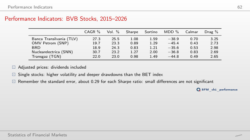
                                                    Slide 62: Performance Indicators: BVB Stocks, 2015–2026
                                                    Slide 62

                                                    Performance indicators; Sharpe with its standard error in brackets

                                                    Duration of the maximum-drawdown episode, all ten series

                                                    Worked example: the maximum drawdown and the Calmar ratio

                                                    \[\text{Calmar} = \frac{\text{CAGR}}{|\text{MDD}|}, \qquad \text{CAGR} = \Big(\frac{P_T}{P_0}\Big)^{1/Y} - 1\]
                                                        Question for the room Over 2015–2026, Nuclearelectrica has the highest Calmar ratio among the BVB stocks (0.83). The ▶ button moves the start of the sample. With the start in 2022, which BVB stock has the highest Calmar ratio?
                                                        Answer

                                                        OMV Petrom (SNP), 1.96: CAGR 38.0% and an MDD of only −19.3%. Transgaz has the highest CAGR (47.6%), but its MDD of −34.5% gives a Calmar ratio of 1.38. Nuclearelectrica drops to 0.40. The denominator is a single episode, so the Calmar ratio changes a lot with the period.

                                                        Risk and Return, 2015–2026
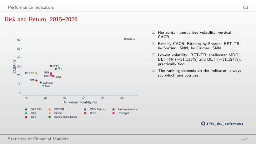
                                                        Slide 63: Risk and Return, 2015–2026
                                                        Slide 63
                                                          Question for the room Over 2015–2026, Bitcoin has the highest CAGR. The ▶ button moves the start of the sample. With the start in 2018, which asset has the highest CAGR?
                                                          Answer

                                                          Nuclearelectrica (SNN), with 40.7% a year; SNN also has the highest Sharpe, Sortino and Calmar ratios in this sample. The CAGR of Bitcoin falls from 60.6% to 22.7%, because the sample starts two weeks after the peak of 16 December 2017. The ranking depends on the indicator and on the period.

                                                          EODHD daily prices up to 18 September 2026: indices and Bitcoin at the close, BVB stocks adjusted for dividends and corporate actions; the BNR EUR/RON reference rate. Comparison period: from 2015; S&P 500 from 2000, BET from 1997 and Bitcoin from 2014 over the full history. Weekly and monthly returns (the last price of each week or month), a risk-free rate other than 0 and the TLV variant without the days of 30 and 31 May 2016 are extra computations on the same prices.