

Statistics of Financial Markets

Chapter 15 · Systemic Risk

The slide of the lecture is on the left, the same figure or table on the right, computed in the browser from the same data. The ▶ button moves the parameter step by step; the tables and worked examples are recomputed with it. Abbreviations: VaR (value at risk), CoVaR (the VaR of the system conditional on an institution), ΔCoVaR (the institution’s contribution to CoVaR), ES (expected shortfall), MES (marginal expected shortfall), LRMES (long-run MES), SRISK (the capital shortfall in a crisis), OLS (ordinary least squares), DGC (degree of Granger causality), VAR (vector autoregression), FROM, TO, NET (the shares received from the other banks, passed to them, and their difference), CET1 (common equity tier 1), G-SIB (global systemically important bank), BCBS (Basel Committee on Banking Supervision), BET (the index of the Bucharest Stock Exchange), VIX (the implied volatility index of the S&P 500), JPM, BAC, C, GS, MS, WFC (JPMorgan Chase, Bank of America, Citigroup, Goldman Sachs, Morgan Stanley, Wells Fargo), DBK, BNP, SAN, INGA, HSBA (Deutsche Bank, BNP Paribas, Santander, ING, HSBC), TLV (Banca Transilvania), BRD (BRD – Groupe Société Générale).

Four Crises in the Data · Correlation and Tail Dependence in Crises · CoVaR and Delta-CoVaR · MES and SRISK · Networks of Banks · Macroprudential Policy

Four Crises in the Data

Bank Portfolios since 2005
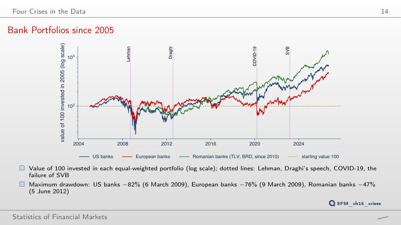
Slide 14: Bank Portfolios since 2005
Slide 14
    Question for the room ▶ moves the investment of the 100 units to the start of 2010 (extra run). What is the maximum drawdown of the US bank portfolio?
    Answer

    −51%, on 23 November 2011, against −82% with the 2005 investment: the March 2009 trough is no longer in the sample. The maximum drawdown depends on the start of the sample; for the European banks the deepest point after 2010 is 21 April 2020 (−61%).

    Four Episodes Side by Side
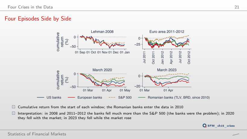
    Slide 21: Four Episodes Side by Side
    Slide 21
      Question for the room ▶ moves the start of each window 30 days later (extra run). What becomes of the minimum of the US banks in the March 2020 episode?
      Answer

      −10.8% instead of −47.6%: the window starts on 15 March 2020, after most of the fall, and the portfolio ends at +16.9%. The cumulative return is measured from the start of the window, so the comparison of episodes depends on that date.

      Correlation and Tail Dependence in Crises

      Correlation between Banks in Crises
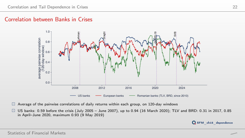
      Slide 22: Correlation between Banks in Crises
      Slide 22
        Question for the room With a 60-day window (▶, extra run), where does the maximum correlation of TLV and BRD go?
        Answer

        To 0.96, on 6 February 2019, still outside any crisis (with 120 days: 0.93 on 9 May 2019). For a single pair of stocks a short window gives larger extremes; the maximum of the US banks stays on 16 March 2020 (0.95).

        Interpretation: Limits of Diversification in Crises
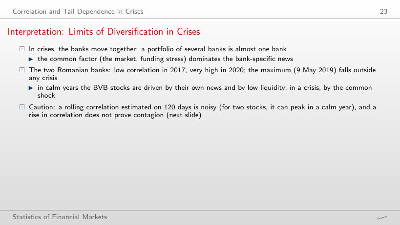
        Slide 23: Interpretation: Limits of Diversification in Crises
        Slide 23

        Mean of the average pairwise correlation by period (the numbers of the previous slide)

          Question for the room ▶ goes through the years 2005–2026. In which year is the yearly mean of the TLV–BRD correlation highest?
          Answer

          In 2019: 0.80, above 2020 (0.76) and 2011 (0.56). The 120-day correlation of two stocks is noisy and can peak in a calm year, as the daily maximum of 9 May 2019 also shows.

          Contagion and Interdependence: Forbes and Rigobon (2/2)
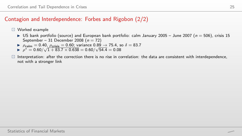
          Slide 25: Contagion and Interdependence: Forbes and Rigobon (2/2)
          Slide 25

          Worked example: the Forbes–Rigobon correction

          \[\rho^* = \frac{\rho}{\sqrt{1 + \delta(1 - \rho^2)}}, \qquad \delta = \frac{\sigma^2_{\text{crisis}}}{\sigma^2_{\text{calm}}} - 1\]
              Question for the room ▶ picks the March 2020 crisis (extra run). Does the corrected correlation ρ* exceed the calm-period correlation of 0.40?
              Answer

              No: ρ_crisis = 0.74, but the variance of the US portfolio rises 47-fold (δ = 46.0), so ρ* = 0.74/√(1 + 46.0 × 0.451) = 0.16. Of the four windows only March 2023 gives ρ* = 0.42, just above 0.40, because volatility rose little (δ = 3.7).

              Tail Dependence of Banks and Markets
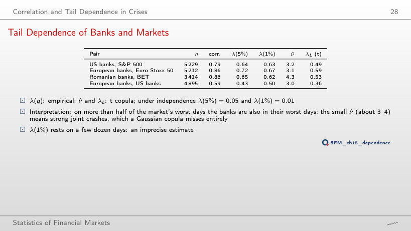
              Slide 28: Tail Dependence of Banks and Markets
              Slide 28

              Tail dependence (the table of the slide and λ(q) at the chosen level)

                Question for the room ▶ lowers q to 0.5% (extra run). What happens to λ(q) for the US banks and the S&P 500?
                Answer

                It rises to 0.73, from 0.64 at 5%; under independence it would be 0.005. The estimate rests on the 26 worst days of the S&P 500, so it is imprecise: for the European banks λ(0.5%) falls to 0.58.

                Joint Large Losses
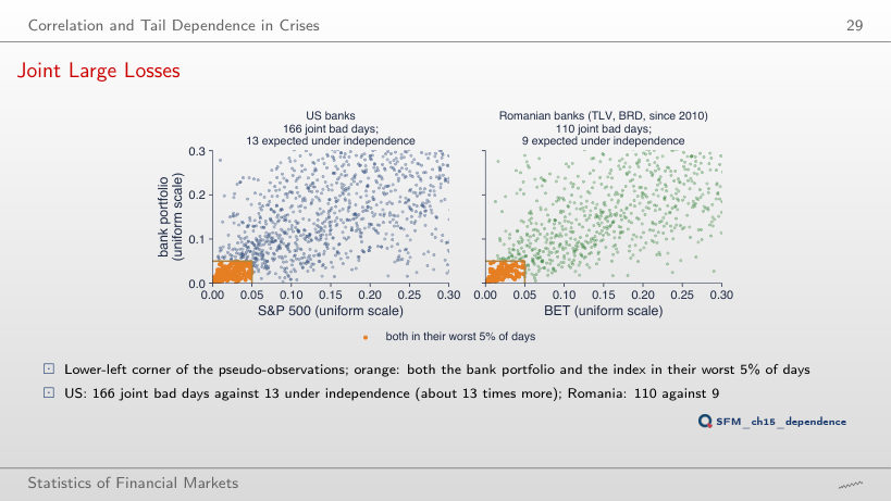
                Slide 29: Joint Large Losses
                Slide 29
                  Question for the room At q = 1% (▶, extra run), how many times as many joint bad days do the US banks and the S&P 500 have as under independence?
                  Answer

                  About 63 times: 33 days against q²n = 0.0001 × 5,229 = 0.52, against 12.7 times at q = 5%. The ratio grows towards the tail: very bad days come together.

                  CoVaR and Delta-CoVaR

                  Worked Example: JPMorgan Chase and the S&P 500
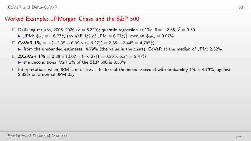
                  Slide 33: Worked Example: JPMorgan Chase and the S&P 500
                  Slide 33

                  Worked example: CoVaR from the quantile regression

                  \[\mathrm{CoVaR}_\alpha = -\big(\hat a + \hat b\,\hat q_\alpha(X^i)\big), \qquad \Delta\mathrm{CoVaR}_\alpha = \hat b\,\big(\hat q_{50\%}(X^i) - \hat q_\alpha(X^i)\big)\]
                      Question for the room ▶ moves to α = 5% (extra run). Is the CoVaR 5% of the S&P 500 conditional on JPM larger or smaller than 4.79%?
                      Answer

                      Smaller: 2.45%. The JPM quantile (−3.07%) and the intercept (−1.26) are less extreme, and the slope stays 0.39; ΔCoVaR 5% = 1.22%, about half of 2.47%.

                      CoVaR: a Graphical Illustration
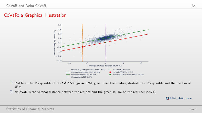
                      Slide 34: CoVaR: a Graphical Illustration
                      Slide 34
                        Question for the room ▶ goes through α = 2.5%, 5% and 10% (extra run). How does the slope b̂ of the red line change for JPM?
                        Answer

                        Hardly at all: 0.385, 0.390 and 0.401, against 0.390 at 1% and 0.398 at the median. The intercept moves, from −2.35 to −0.86: the lines are almost parallel, so ΔCoVaR falls because the distance between the JPM quantiles falls.

                        ΔCoVaR 1% of 13 Banks
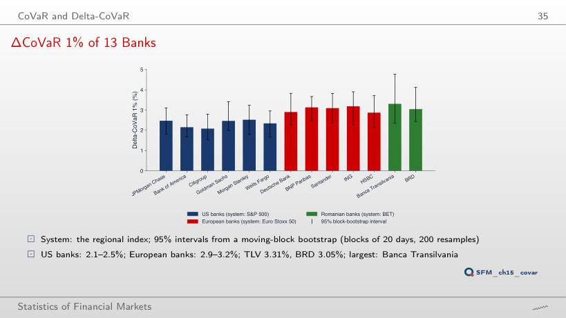
                        Slide 35: ΔCoVaR 1% of 13 Banks
                        Slide 35
                          Question for the room At the 5% level (▶, extra run), which group of banks has the largest ΔCoVaR?
                          Answer

                          Still the European banks: 1.43–1.68% (Santander 1.68%), against 1.12–1.33% for the US banks; TLV 1.51%, BRD 1.45%. At 1% the largest value was TLV’s (3.31%).

                          Interpretation of ΔCoVaR
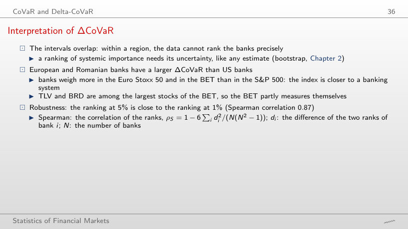
                          Slide 36: Interpretation of ΔCoVaR
                          Slide 36

                          CoVaR and ΔCoVaR 1% of the 13 banks (the numbers of the previous chart) and ΔCoVaR at α₂

                            Question for the room With α₂ = 10% (▶, extra run), what is the Spearman correlation between the ranking of the banks at 1% and at 10%?
                            Answer

                            0.84, against 0.87 at 5% and at 2.5%: the ranking stays close; the level of ΔCoVaR changes (0.74–1.20% at 10%), not the ranking.

                            Worked Example: Banca Transilvania and the BET
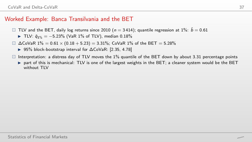
                            Slide 37: Worked Example: Banca Transilvania and the BET
                            Slide 37

                            Worked example: ΔCoVaR between the median and the stress state

                            \[\Delta\mathrm{CoVaR}_\alpha = \mathrm{CoVaR}^{sys|X^i = q_\alpha}_\alpha - \mathrm{CoVaR}^{sys|X^i = q_{50\%}}_\alpha = \hat b\,\big(\hat q_{50\%} - \hat q_\alpha\big)\]
                                Question for the room At α = 5% (▶, extra run), what is the ΔCoVaR of TLV?
                                Answer

                                1.51%, less than half of 3.31%: the slope falls from 0.611 to 0.542 and the distance between TLV’s median and its quantile falls from 5.41 to 2.79 percentage points; 0.542 × 2.79 = 1.51.

                                VaR and ΔCoVaR Compared
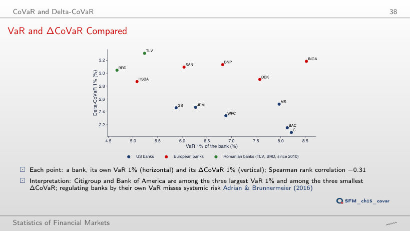
                                Slide 38: VaR and ΔCoVaR Compared
                                Slide 38
                                  Question for the room At the 10% level (▶, extra run), does the Spearman correlation between VaR and ΔCoVaR stay negative?
                                  Answer

                                  No: it becomes +0.20 (at 2.5%: −0.13; at 5%: +0.03). With 13 banks none of these correlations, not even −0.31 at 1% (p = 0.31), is significant at 5%; what remains is that a bank’s own VaR does not rank the banks by ΔCoVaR.

                                  ΔCoVaR 1% through Time
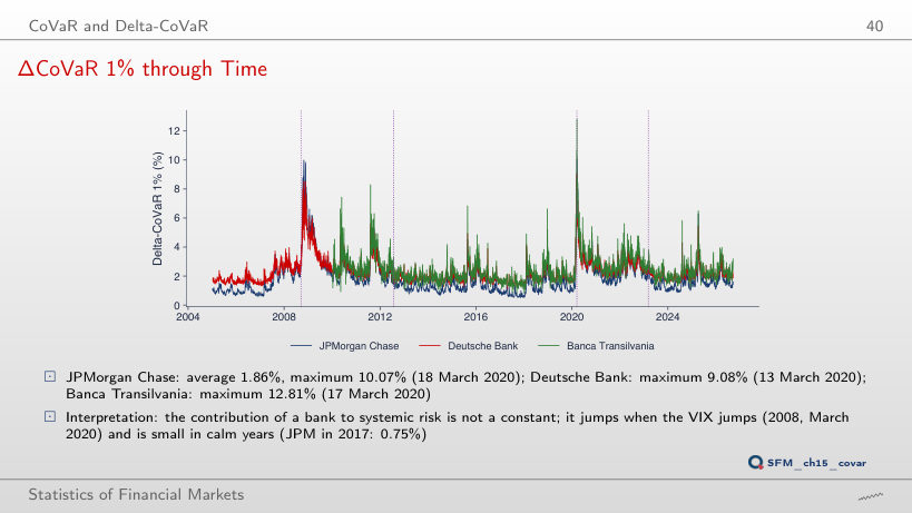
                                  Slide 40: ΔCoVaR 1% through Time
                                  Slide 40
                                    Question for the room At α = 2.5% (▶, extra run), when does the ΔCoVaR of JPMorgan Chase peak?
                                    Answer

                                    On 28 October 2008 (7.58%), not in March 2020 as at 1% and 5%; in March 2020 it reaches 7.52%. The two peaks are almost equal, so the date of the maximum depends on α.

                                    MES and SRISK

                                    Worked Example: MES from Ten Days
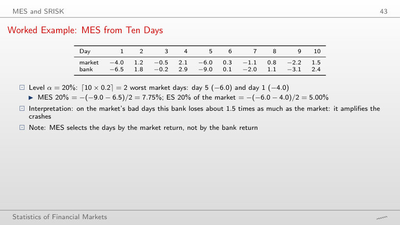
                                    Slide 43: Worked Example: MES from Ten Days
                                    Slide 43

                                    Worked example: MES as the average return of the bank on the market’s tail days

                                    \[\mathrm{MES}_\alpha = -\frac{1}{k}\sum_{t \in \text{worst } k \text{ market days}} X^i_t, \qquad k = \lceil n\alpha \rceil\]
                                        Question for the room At α = 30% (▶), what is MES?
                                        Answer

                                        6.20% = −(−9.0 − 6.5 − 3.1)/3: day 9 is added (market −2.2%, bank −3.1%). The ES 30% of the market = 4.07%, and MES falls from 7.75% because the third day is less extreme.

                                        MES 5% of 13 Banks
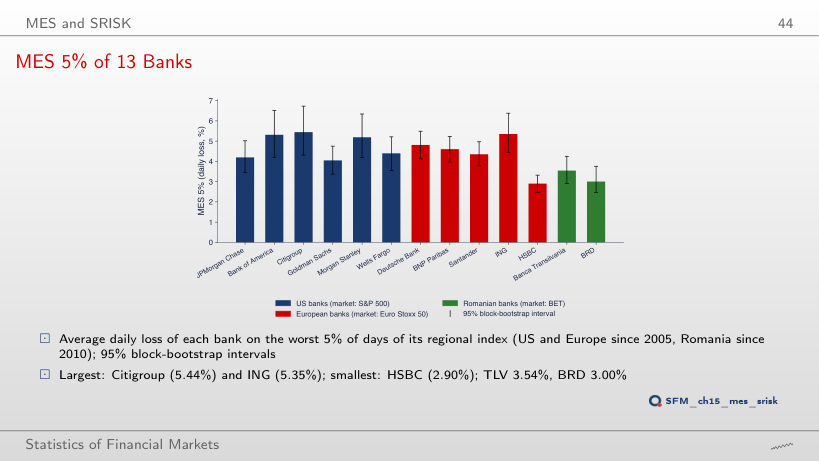
                                        Slide 44: MES 5% of 13 Banks
                                        Slide 44
                                          Question for the room At the 1% level (▶, extra run), which bank has the largest MES?
                                          Answer

                                          Citigroup, 10.64%, almost tied with Bank of America (10.62%); HSBC stays the smallest (4.86%). At 1% MES rests on 53 days of the S&P 500.

                                          Interpretation: MES and ΔCoVaR
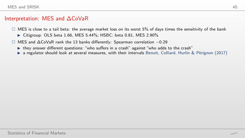
                                          Slide 45: Interpretation: MES and ΔCoVaR
                                          Slide 45

                                          MES, OLS beta, ES of the market, LRMES and the break-even leverage (the numbers of the slides)

                                            Question for the room At the 1% level (▶, extra run), how does the Spearman correlation between MES and ΔCoVaR 1% change?
                                            Answer

                                            It becomes more negative: −0.58, against −0.29 at 5%. The two measures answer different questions, and at the same 1% level their rankings differ even more.

                                            Case Study: MES and the Bank Losses of 2008
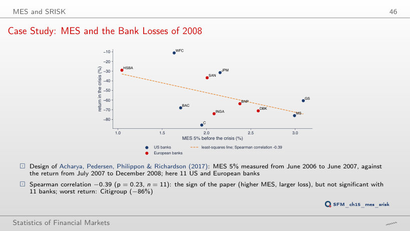
                                            Slide 46: Case Study: MES and the Bank Losses of 2008
                                            Slide 46
                                              Question for the room At the 1% level (▶, extra run), does the Spearman correlation between MES and the 2007–2008 loss become significant?
                                              Answer

                                              No: −0.37 (p = 0.26); at 10%: −0.41 (p = 0.21). The sign is the paper’s, but with 11 banks it is not separated from noise.

                                              Long-Run MES (LRMES)
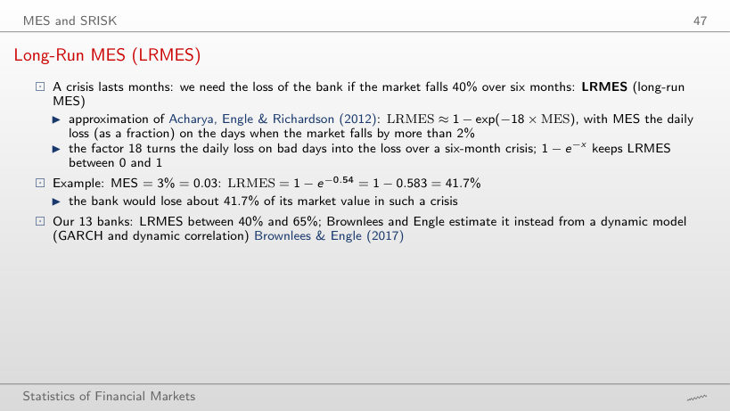
                                              Slide 47: Long-Run MES (LRMES)
                                              Slide 47

                                              Worked example: from MES to LRMES

                                              \[\mathrm{LRMES} \approx 1 - \exp(-18 \times \mathrm{MES})\]
                                                  Question for the room At MES = 6% (▶), what is LRMES?
                                                  Answer

                                                  66.0% = 1 − e^(−1.08), not 83.4% = 2 × 41.7%: the function 1 − e^(−x) rises more and more slowly and stays below 100%.

                                                  SRISK: the Capital Shortfall in a Crisis
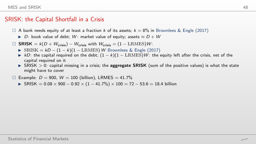
                                                  Slide 48: SRISK: the Capital Shortfall in a Crisis
                                                  Slide 48

                                                  Worked example: SRISK

                                                  \[\mathrm{SRISK} = kD - (1 - k)(1 - \mathrm{LRMES})\,W\]
                                                      Question for the room With W = 50 billion (▶), what is SRISK?
                                                      Answer

                                                      45.2 billion = 72 − 0.92 × 0.583 × 50 = 72 − 26.8. The leverage L = 950/50 = 19 is far above L* = 7.7: a fall in the market value of equity increases the shortfall.

                                                      SRISK and Leverage
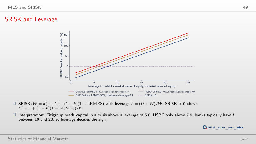
                                                      Slide 49: SRISK and Leverage
                                                      Slide 49
                                                        Question for the room With k = 5.5% (▶, the European rule of the next slide), above what leverage does Citigroup need capital in a crisis?
                                                        Answer

                                                        6.9, against 5.0 with k = 8%: a smaller k requires less capital, so the threshold L* = 1 + 0.945 × 0.345/0.055 rises. For HSBC the threshold rises to 11.3.

                                                        Networks of Banks

                                                        Granger Networks through Time
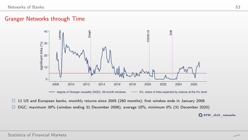
                                                        Slide 53: Granger Networks through Time
                                                        Slide 53
                                                          Question for the room With 60-month windows (▶, extra run), what is the maximum DGC?
                                                          Answer

                                                          35.5% (the window that ends in January 2010), against 39.1% with 36 months; the mean rises from 9.6% to 12.0%, because 2007–2009 stays in more windows.

                                                          Two Networks: 2007–2009 and 2017–2019
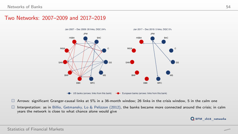
                                                          Slide 54: Two Networks: 2007–2009 and 2017–2019
                                                          Slide 54
                                                            Question for the room ▶ moves both windows 12 months earlier (2006–2008 and 2016–2018). How many links does the crisis window have?
                                                            Answer

                                                            43 (DGC 39%), against 26 in 2007–2009; the calm window has 7. The window that ends in December 2008 is the maximum of the previous chart.

                                                            Diebold–Yilmaz Connectedness
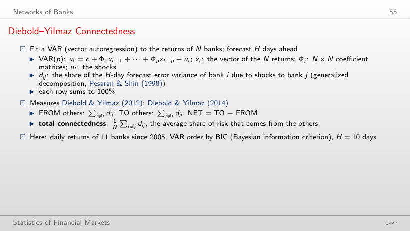
                                                            Slide 55: Diebold–Yilmaz Connectedness
                                                            Slide 55

                                                            Worked example: a share of the variance decomposition and the total connectedness

                                                            \[\mathrm{FROM}_i = \sum_{j \ne i} d_{ij} = 100 - d_{ii}, \quad \mathrm{TO}_i = \sum_{j \ne i} d_{ji}, \quad \text{total} = \frac{1}{N}\sum_{i \ne j} d_{ij}\]
                                                                Question for the room With H = 1 day (▶), what is FROM for JPMorgan Chase?
                                                                Answer

                                                                80.6%, practically as at H = 10 (80.65%); the total connectedness is 78.0% against 78.3%. Daily returns are almost unpredictable, so the decomposition comes almost entirely from the correlation of same-day shocks, not from the VAR dynamics.

                                                                The Connectedness Table
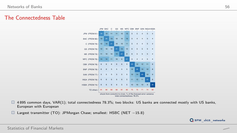
                                                                Slide 56: The Connectedness Table
                                                                Slide 56
                                                                  Question for the room With H = 30 days (▶), how does the total connectedness change?
                                                                  Answer

                                                                  It stays 78.3%: from H = 5 on, the value no longer changes at the first decimal. The VAR(1) coefficients of daily returns are small, so the effects of a shock die out within a few days.

                                                                  Interpretation of the Connectedness Table
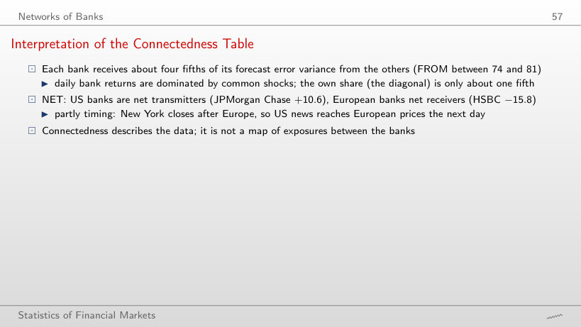
                                                                  Slide 57: Interpretation of the Connectedness Table
                                                                  Slide 57

                                                                  Own share, FROM, TO and NET (in %, horizon of 10 days)

                                                                    Question for the room In the 2020–2026 sub-period (▶, extra run), which bank has the most negative NET?
                                                                    Answer

                                                                    HSBC, −20.1, as over the whole period; the US banks stay net transmitters (JPMorgan Chase +8.8, Bank of America +11.3), and the total connectedness is 80.2%.

                                                                    Total Connectedness through Time
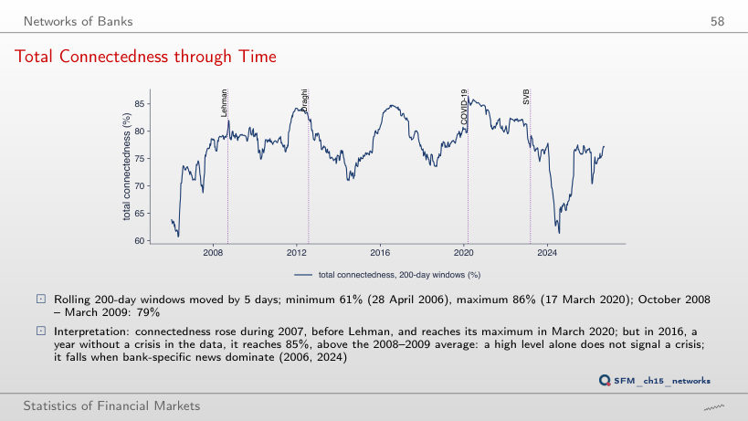
                                                                    Slide 58: Total Connectedness through Time
                                                                    Slide 58
                                                                      Question for the room With 100-day windows (▶, extra run), does the maximum of the total connectedness stay in March 2020?
                                                                      Answer

                                                                      Yes: 87.9% on 17 March 2020. The 2016 maximum rises to 86.0% and the minimum falls to 54.5% (20 May 2024): short windows give larger extremes in both directions.

                                                                      Macroprudential Policy

                                                                      Basel III Capital Buffers
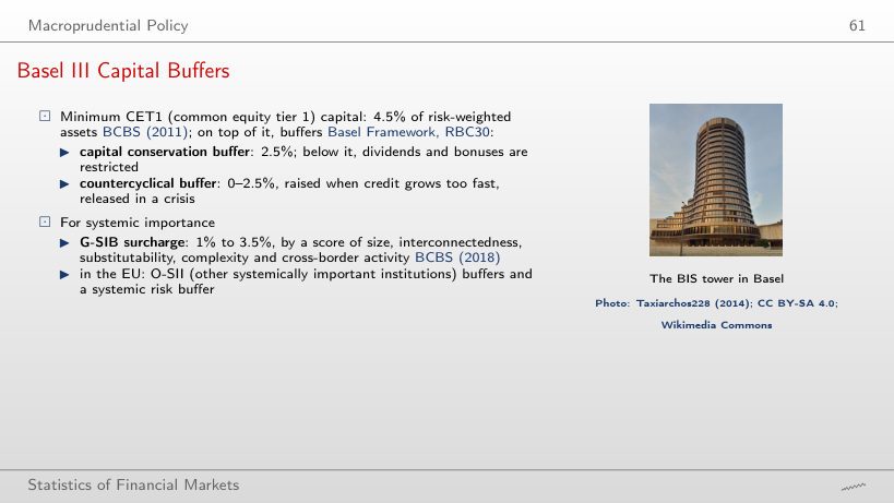
                                                                      Slide 61: Basel III Capital Buffers
                                                                      Slide 61

                                                                      Worked example: the CET1 requirement of a bank

                                                                      \[\text{CET1 required} = 4.5\% + 2.5\% + \text{countercyclical} + \text{G-SIB surcharge}\]
                                                                          Question for the room At the end of ▶ the countercyclical buffer reaches 2.5%. What is the CET1 requirement of a G-SIB with the minimum surcharge of 1%?
                                                                          Answer

                                                                          10.5% = 4.5 + 2.5 + 2.5 + 1 of risk-weighted assets (BCBS (2011); BCBS (2018)). With the maximum surcharge of 3.5% it would be 13%.

                                                                          Course data in data/market (EODHD, January 2005 – 18 September 2026): daily adjusted closes of the 13 banks and the closes of the S&P 500, Euro Stoxx 50 and BET; the Romanian banks since 2010. The quantile-regression coefficients, the block-bootstrap intervals of ΔCoVaR 1% and MES 5%, the t-copula parameters, the time-varying ΔCoVaR and the rolling total connectedness come from the code of the chapter (Quantlets/Ch_15). From the prices the browser recomputes the returns, the bank portfolios, the episodes, the correlations, the Forbes–Rigobon test, the empirical tail dependence, the quantiles, CoVaR and ΔCoVaR, MES, LRMES, SRISK, the Granger networks and the Diebold–Yilmaz table. Other levels α, windows, thresholds, periods and horizons are extra runs of the same code. The examples of MES from ten days, LRMES, SRISK and the Basel III buffers use the numbers of the slides; the capital requirements follow BCBS (2011) and BCBS (2018).