

Statistics of Financial Markets

Chapter 6 · Model Selection and Risk Management

The slide of the lecture is on the left, the same figure or table on the right, computed in the browser from the same data. The ▶ button moves the parameter step by step; the tables and worked examples are recomputed with it.

Candidate Distributions · Review of Maximum Likelihood Estimation · Nested Models: the Likelihood-Ratio Test · Information Criteria: AIC and BIC · Goodness-of-Fit Tests · PP and QQ Plots · Comparing the Models on VaR 1% · Out of Sample: Validation and Overfitting · Model Uncertainty

Candidate Distributions

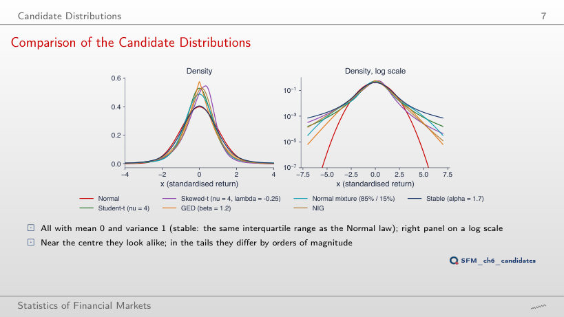
Comparison of the Candidate Distributions
Slide 7: Comparison of the Candidate Distributions
Slide 7

P(X < −x) for each candidate (mean 0, variance 1)

    Question for the room At x = 4, the Student-t distribution (ν = 4) gives a probability P(X < −4) 76 times that of the Normal distribution. The ▶ button moves the threshold from 2 to 6. How many times larger is the Student-t probability at x = 6?
    Answer

    About 536,000 times: 5.3 × 10⁻⁴ against 9.9 × 10⁻¹⁰. At x = 2 the two probabilities are almost equal (ratio 1.0), at x = 3 the ratio is 4.9, at x = 5 it is 3,682. The Normal tail falls as e−x²/2, the Student-t tail as a power of x, so the ratio grows ever faster with the threshold. The mean and the variance are the same; the difference lies only in the tail, where VaR 1% sits.

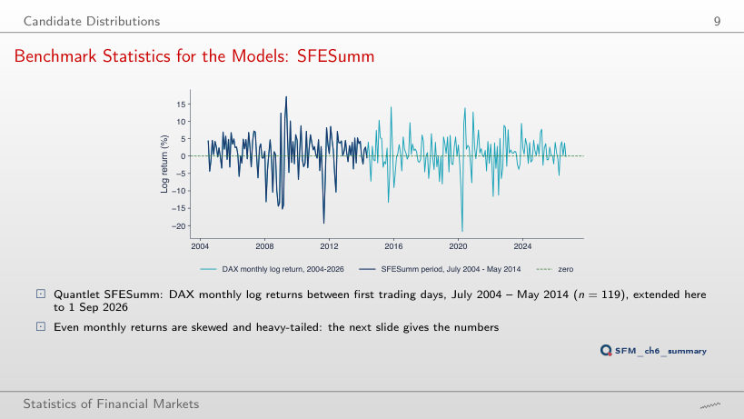
    Benchmark Statistics for the Models: SFESumm
    Slide 9: Benchmark Statistics for the Models: SFESumm
    Slide 9

    Summary statistics, DAX monthly log returns (%)

      Question for the room The kurtosis of the DAX monthly returns is 4.60 on the SFESumm sample (July 2004 – May 2014) and 5.06 on 2004–2026. The ▶ button extends the sample one year at a time. Does the kurtosis rise gradually as years are added?
      Answer

      No. Between 2014 and 2019 it falls, to 4.30 in May 2016, because the months added are calm. It jumps to 4.93 when the return from early March to early April 2020 enters, −21.70%, the new minimum of the sample (the old one was −19.35%). The kurtosis depends on a few extreme months, not on the number of months. On 2004–2026 the skewness stays negative (−0.72), and the Jarque–Bera test rejects Normality with JB = 70.2.

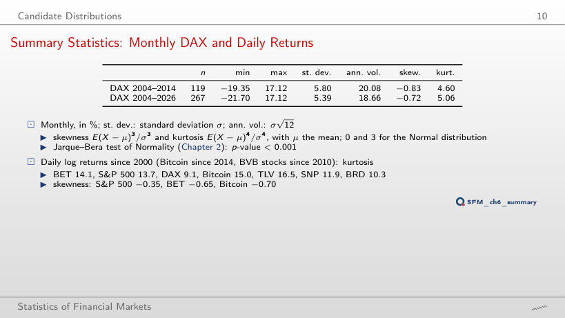
      Summary Statistics: Monthly DAX and Daily Returns
      Slide 10: Summary Statistics: Monthly DAX and Daily Returns
      Slide 10

      Daily log returns (%)

      Worked example: the Jarque–Bera test

      \[JB = \frac{n}{6}\Big[S^2 + \frac{(K-3)^2}{4}\Big] \approx \chi^2(2)\]
          Question for the room Without the two erroneous days of May 2016, the kurtosis of the TLV daily returns is 16.5. What does it become if the two days, −15.0% and +20.5%, stay in the data?
          Answer

          20.5. Kurtosis uses the fourth power of the deviations from the mean, so two extreme days move it a lot, even though their sum, +5.5%, is small. The skewness moves from −0.87 to −0.58. In the lecture, ν̂ of the Student-t falls from 3.44 to 3.33, and the AIC ranking does not change (Student-t wins in both cases). The JB of TLV rises too, because (K − 3)² rises.

          Review of Maximum Likelihood Estimation

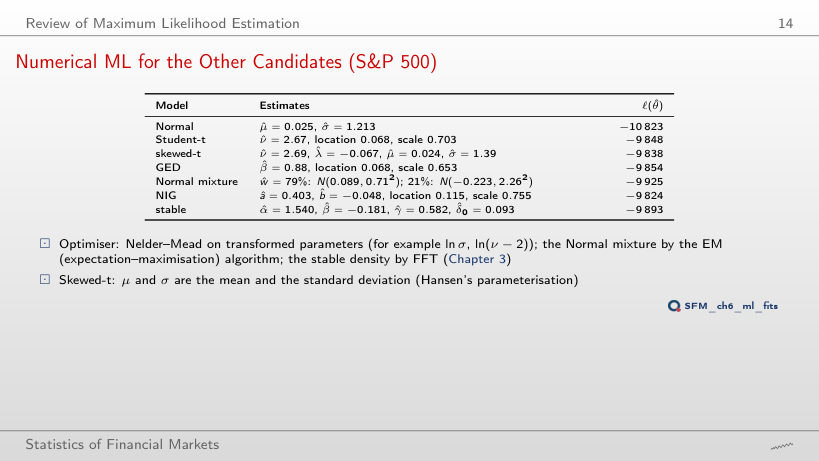
          Numerical ML for the Other Candidates (S&P 500)
          Slide 14: Numerical ML for the Other Candidates (S&P 500)
          Slide 14

          ML estimates and the maximised log-likelihood

          Worked example: the Normal model, step by step

          \[\ell(\hat\mu, \hat\sigma) = -\frac{n}{2}\big[\ln(2\pi\hat\sigma^2) + 1\big], \quad \hat\sigma^2 = \frac{1}{n}\sum_t (r_t - \bar r)^2\]
              Question for the room For the S&P 500, ν̂ of the Student-t distribution is 2.67. Bitcoin has a larger sample kurtosis (15.0 against 13.7). Is the ν̂ of Bitcoin smaller or larger?
              Answer

              Smaller: 2.23, the smallest of the seven series, hence the heaviest tail. BET has 2.43, DAX 3.09, BRD 4.67. A ν̂ close to 2 means a variance that is barely finite. The large standard deviation of Bitcoin (3.5% per day) goes into the scale, not into ν: the Student-t scale of Bitcoin is 1.85, and the implied standard deviation, scale·√(ν/(ν − 2)), is 5.75%, above the sample standard deviation (3.49%), because ν̂ is close to 2.

              Precision of ν: the Profile Log-Likelihood
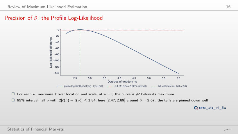
              Slide 16: Precision of ν: the Profile Log-Likelihood
              Slide 16

              Worked example: is the tested ν inside the interval?

              \[LR(\nu) = 2\big[\ell(\hat\nu) - \ell(\nu)\big] \le \chi^2_{1-a}(1)\]
                  Question for the room The slide gives the 95% interval for ν of the S&P 500, [2.47, 2.89], where the profile crosses the cut-off. Which points of the grid of step 0.1 used in the chart lie inside the interval?
                  Answer

                  From 2.5 to 2.8. The true end points, 2.47 and 2.89, lie between grid points (2.4–2.5 and 2.8–2.9); a 0.1 grid read directly would give [2.5, 2.8], an interval that is too narrow. The interval is not symmetric around ν̂ = 2.67: 0.20 to the left, 0.22 to the right, because the profile is not a parabola. At ν = 5, the profile log-likelihood is 92.3 below its maximum.

                  Nested Models: the Likelihood-Ratio Test

                  Worked Example: Testing the Skewness Parameter
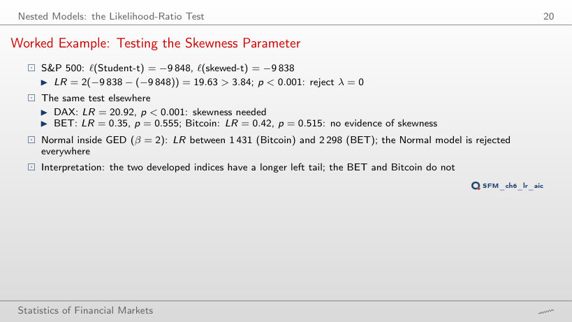
                  Slide 20: Worked Example: Testing the Skewness Parameter
                  Slide 20

                  Worked example: the likelihood-ratio test

                  \[LR = 2\,[\ell_1(\hat\theta_1) - \ell_0(\hat\theta_0)] \approx \chi^2(k_1 - k_0)\]

                    The same test on the seven series

                    The p-value as a function of LR

                      Question for the room For BRD, the test of Student-t inside skewed-t (λ = 0) gives LR = 3.01. Is the skewness parameter needed at 5%?
                      Answer

                      No: 3.01 < 3.84, p = 0.083. The fixed value λ = 0 lies inside the interval (−1, 1), so Wilks' theorem applies and the critical value is 3.84; 2.71 is the boundary value (Normal inside Student-t). AIC still prefers skewed-t (ΔAIC of Student-t: 1.0), because AIC is not a test: it charges 2 for a parameter, and LR > 2. The skewness is significant only for the S&P 500 (LR = 19.63) and the DAX (20.92).

                      Non-Nested Models: the Vuong Test
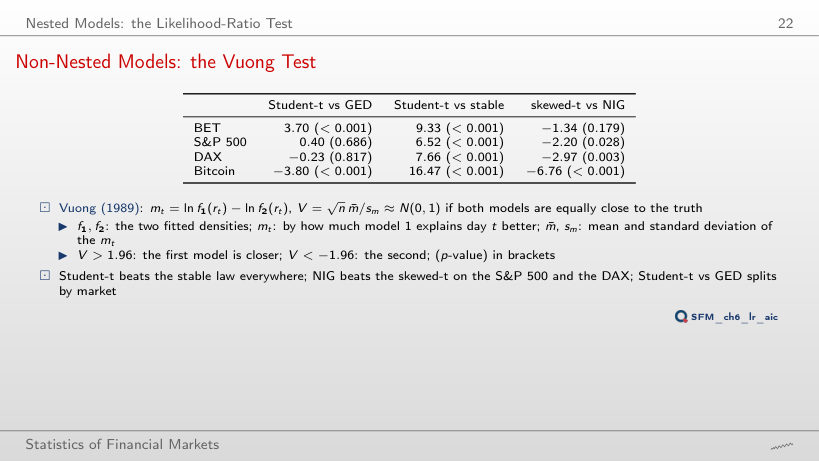
                      Slide 22: Non-Nested Models: the Vuong Test
                      Slide 22

                      Worked example: the Vuong statistic

                      \[m_t = \ln f_1(r_t) - \ln f_2(r_t), \qquad V = \frac{\sqrt{n}\,\bar m}{s_m} \approx N(0, 1)\]

                        The statistic V and its p-value on the seven series

                        Cumulative sum of the daily differences mt

                          Question for the room On the slide, Student-t is preferred to the stable distribution on all four markets. For BRD, V = 1.89. Is the preference significant at 5%?
                          Answer

                          No: |V| = 1.89 < 1.96, p = 0.059. Student-t explains the BRD days better on average, but the difference is not separated from noise. The day with the largest |mt| is 19 December 2018 (mt = −2.48: the stable distribution explains this fall better). For TLV and SNP, V = 3.77 and 4.16. The sum of the daily differences is exactly the difference of the log-likelihoods, ℓ(Student-t) − ℓ(stable).

                          Information Criteria: AIC and BIC

                          Worked Example: Seven Models for the S&P 500
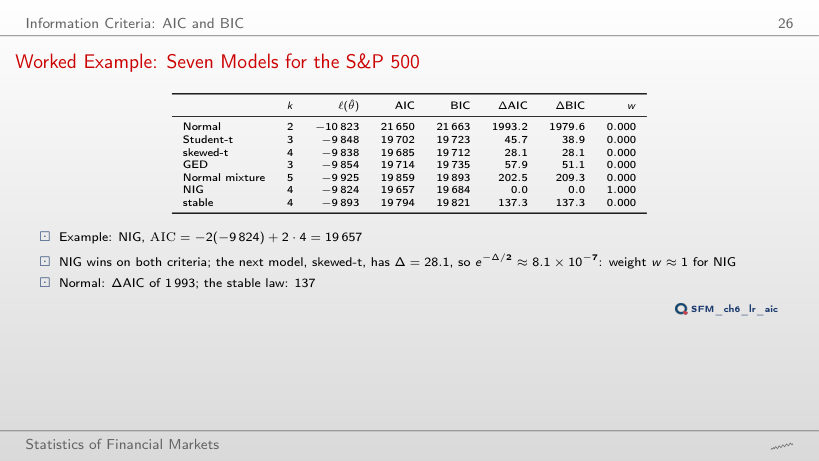
                          Slide 26: Worked Example: Seven Models for the S&P 500
                          Slide 26

                          Worked example: AIC, BIC and the Akaike weight

                          \[\mathrm{AIC} = -2\ell(\hat\theta) + 2k, \quad \mathrm{BIC} = -2\ell(\hat\theta) + k\ln n, \quad w_i = \frac{e^{-\Delta_i/2}}{\sum_j e^{-\Delta_j/2}}\]
                              Question for the room For BRD, AIC prefers skewed-t, and Student-t has ΔAIC = 1.0. What Akaike weights do the two models get?
                              Answer

                              0.62 for skewed-t and 0.38 for Student-t (the other five models have weights of practically zero): w = e−Δ/2/Σ e−Δj/2, with e−0.5 = 0.61. A difference of 1 leaves both models plausible; AIC is not a test. With BIC weights the order reverses: 0.93 for Student-t.

                              ΔAIC across Seven Series
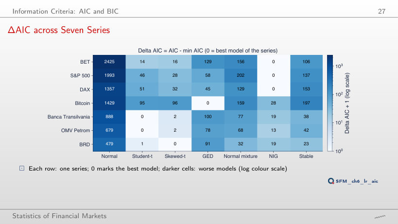
                              Slide 27: ΔAIC across Seven Series
                              Slide 27

                              The best model under each criterion

                                Question for the room For BRD, AIC prefers skewed-t (ΔAIC of Student-t: 1.0). The ▶ button switches to BIC. Which model does BIC prefer?
                                Answer

                                Student-t, with ΔBIC = 5.2 for skewed-t. BIC charges the extra parameter ln 3,771 = 8.24, more than the gain in fit (LR = 3.01). For TLV and SNP, both criteria choose Student-t; for BET, S&P 500 and DAX, NIG; for Bitcoin, GED. The Normal model has ΔBIC between 472 and 2,412.

                                Goodness-of-Fit Tests

                                Worked Example: KS on Five Returns
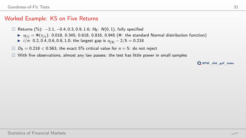
                                Slide 31: Worked Example: KS on Five Returns
                                Slide 31

                                Worked example: the KS statistic

                                \[D_n = \max_i \max\Big\{\frac{i}{n} - u_{(i)},\ u_{(i)} - \frac{i-1}{n}\Big\}, \quad u_{(i)} = F(r_{(i)})\]
                                    Question for the room With H0: N(0, 1), D5 = 0.218 < 0.563. The ▶ button moves σ of the null from 0.5 to 2. For which σ in this range does the test reject at 5%?
                                    Answer

                                    None: D5 lies between 0.188 (σ = 1.4) and 0.364 (σ = 0.5), always below 0.563. With five observations, the test cannot separate a standard deviation of 0.5% from one of 2%: its power is very low. With μ and σ estimated from the five returns (Lilliefors), D5 = 0.175, and the critical value falls to 0.351 (the lecture's simulation, as on the slide).

                                    Low Power of KS in the Tails
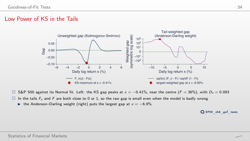
                                    Slide 34: Low Power of KS in the Tails
                                    Slide 34

                                    Worked example: the KS distance at its maximum

                                    \[D_n = \max_i \max\Big\{\frac{i}{n} - u_{(i)},\ u_{(i)} - \frac{i-1}{n}\Big\}, \qquad c_{0.05} = \frac{1.358}{\sqrt n}\]
                                        Question for the room For the S&P 500, the KS distance between the empirical distribution and the fitted Normal distribution is largest at x = −0.41%, close to the centre. Where is the maximum for Bitcoin?
                                        Answer

                                        Also in the body of the distribution: at x = −1.69% (F = 30%), with Dn = 0.099. For all seven series, the KS maximum lies between x = −1.7% and +1.0%, where the distribution functions are steep. The Anderson–Darling weighted distance is largest in the tail: −6.9% for the S&P 500, −20.1% for Bitcoin. KS measures the shape of the body, AD the shape of the tails.

                                        Power of the Three Tests
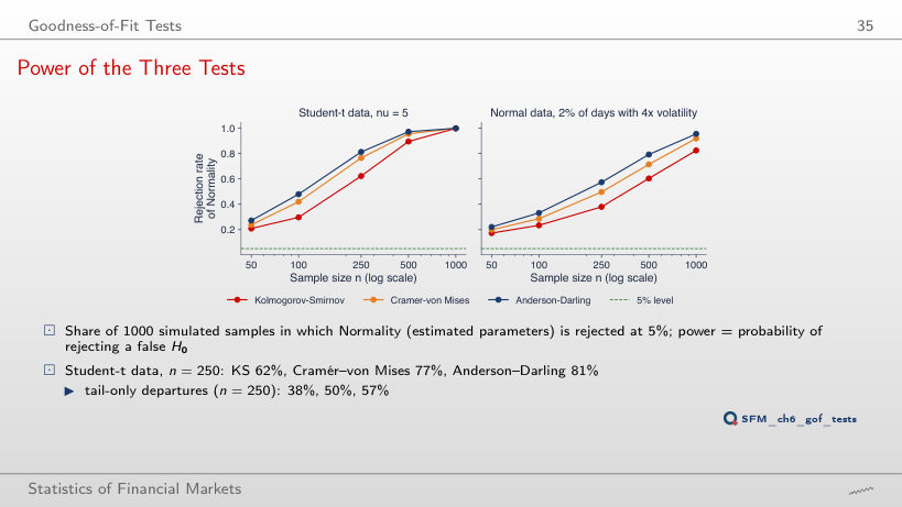
                                        Slide 35: Power of the Three Tests
                                        Slide 35

                                        Power at 5%: Student-t data (ν = 5) and Normal data with 2% of days 4 times as volatile

                                        KS critical values at 5%: estimated parameters (simulation, 4,000 samples) and known F

                                          Question for the room At n = 250, when the departures from the Normal distribution are only in the tails, the power is 38% (KS), 50% (CvM) and 57% (AD). The ▶ button raises n to 1,000. What does the power of the KS test become?
                                          Answer

                                          82.5%, below that of AD (95.6%) and CvM (92.0%). With Student-t data (ν = 5), at n = 1,000 all three reject almost always (99.9%–100%). The AD test puts more weight on the tails, where the departure is. At n = 100, KS rejects Student-t data in only 30% of the samples: a KS test on 100 returns that does not reject the Normal distribution says little about VaR 1%.

                                          EDF Tests on the S&P 500
                                          Slide 36: EDF Tests on the S&P 500
                                          Slide 36

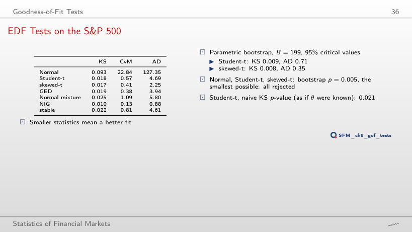
                                          EDF statistics of the fitted models; ranks by AD and by AIC

                                            Question for the room Does the AD statistic rank the S&P 500 models in the same order as AIC?
                                            Answer

                                            Not exactly. By AD: NIG (0.88), skewed-t (2.25), GED (3.94), stable (4.61), Student-t (4.69), Normal mixture (5.80), Normal (127.35). By AIC: NIG, skewed-t, Student-t, GED, stable, Normal mixture, Normal. The first two and the last two places agree; Student-t drops from 3rd to 5th. AD and AIC measure different things: AD the weighted distance between distribution functions, AIC the density at the observed points.

                                            PP and QQ Plots

                                            PP Plots: S&P 500
                                            Slide 39: PP Plots: S&P 500
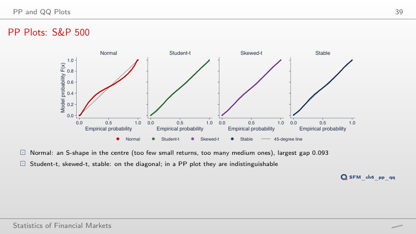
                                            Slide 39
                                              Question for the room In the PP plot of the S&P 500, the largest vertical distance of the Normal model is 0.093. What is it for the Student-t?
                                              Answer

                                              0.018, practically the KS statistic (0.018). Skewed-t has 0.017, the stable distribution 0.022: in the PP plot the three cannot be told apart, although their tails differ by orders of magnitude. The PP plot squeezes the tails into the corners; the QQ plot on the next slide stretches them.

                                              QQ Plots: S&P 500
                                              Slide 40: QQ Plots: S&P 500
                                              Slide 40

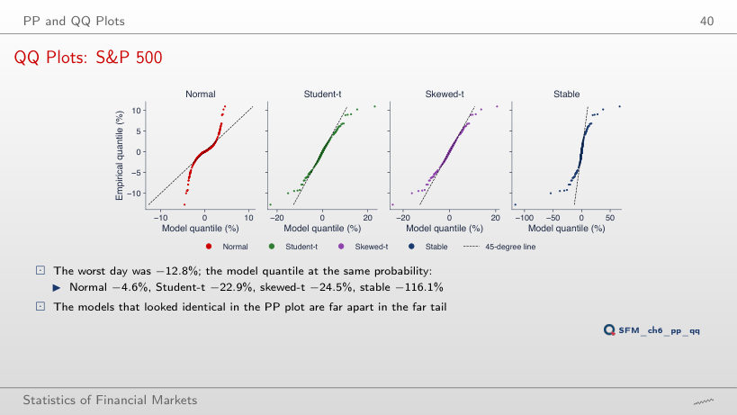
                                              Quantile of each model at the probability of the smallest return, 0.5/n (%)

                                                Question for the room For the S&P 500, the quantile of the stable distribution at the probability of the smallest return (−12.8%) is −116.1%. For Bitcoin, with the smallest return −46.5% (12 March 2020), what does the stable distribution give?
                                                Answer

                                                −385.6%, more than 8 times the observed value. Student-t gives −85.0%, NIG −31.3%, GED −24.2%, the Normal model −12.7%. At the probability 0.5/n = 1.1 × 10⁻⁴, the models differ most and the data hold a single point: the uncertainty is largest there.

                                                QQ Plots for BET, Bitcoin and Banca Transilvania
                                                Slide 41: QQ Plots for BET, Bitcoin and Banca Transilvania
                                                Slide 41
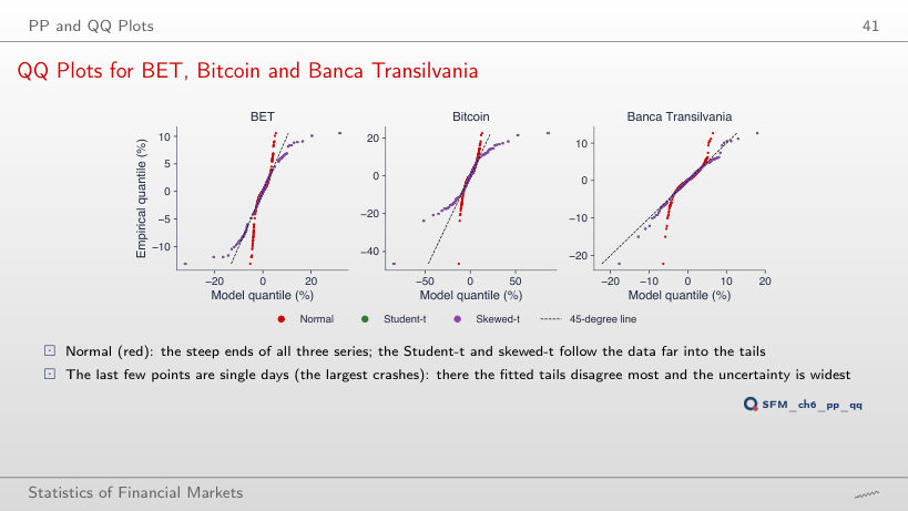
                                                  Question for the room For Bitcoin, the largest daily fall (12 March 2020, −46.5%) has the Student-t quantile −85.0%. The ▶ button moves to the second, third… smallest return. What Student-t quantile does the second smallest return, −23.8%, get?
                                                  Answer

                                                  −51.9%, more than twice the observed return; at the tenth (−15.5%), −22.5%. The Student-t tail fitted to Bitcoin (ν̂ = 2.23) is longer than that of the data. For TLV it is the other way round: the largest fall, −22.2%, has the Student-t quantile −17.8%. The Normal model stays far inside the data for all three series (Bitcoin: −12.7%).

                                                  Comparing the Models on VaR 1%

                                                  VaR 1% and ES 2.5% under Each Model (In Sample)
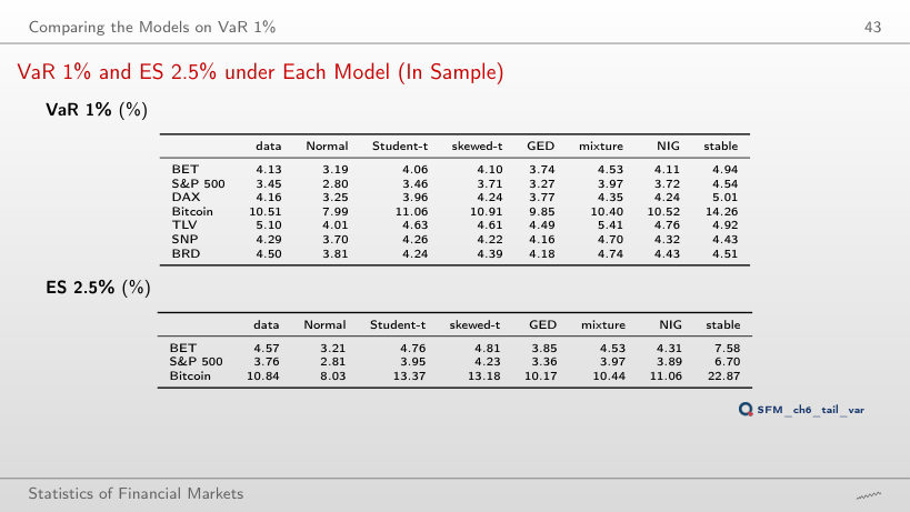
                                                  Slide 43: VaR 1% and ES 2.5% under Each Model (In Sample)
                                                  Slide 43

                                                  Worked example: VaR and ES of the Normal model

                                                  \[\mathrm{VaR}_\alpha = -(\hat\mu + \hat\sigma z_\alpha), \qquad \mathrm{ES}_\alpha = -\hat\mu + \hat\sigma\,\frac{\varphi(z_\alpha)}{\alpha}\]
                                                      Question for the room At VaR 1%, the Normal model gives 2.80% for the S&P 500 and the data 3.45%. The ▶ button goes through the levels. At VaR 0.1%, what do the Normal model and the data give?
                                                      Answer

                                                      The Normal model 3.72%, the data 7.22%: at 0.1% the Normal model covers only half of the loss. Student-t gives 8.58%, NIG 6.98%, the stable distribution 19.70%. At VaR 5% the order reverses: the Normal model gives 1.97%, above the data (1.85%). The Normal ES 2.5% from the formula φ(z)/α (2.81%) equals the value obtained by integrating the quantile.

                                                      Model VaR 1% Relative to the Data
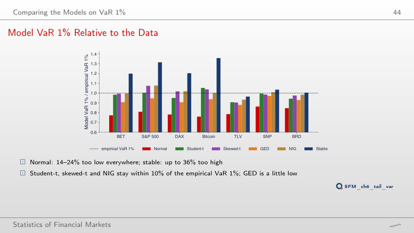
                                                      Slide 44: Model VaR 1% Relative to the Data
                                                      Slide 44
                                                        Question for the room At VaR 1%, the ratio of the Normal VaR to the empirical VaR lies between 0.76 and 0.86 on the seven series. The ▶ button goes through the levels. What does the ratio become at VaR 5%?
                                                        Answer

                                                        Above 1 on every series, between 1.03 (DAX) and 1.16 (BET): at 5% the Normal model overstates the loss. The same standard deviation σ̂ is too large for the body of the distribution and too small for its tail; the two errors cancel somewhere between 2.5% and 5%. At 0.1% the ratio falls to 0.45–0.65.

                                                        The Left Tail on Log-Log Axes (S&P 500)
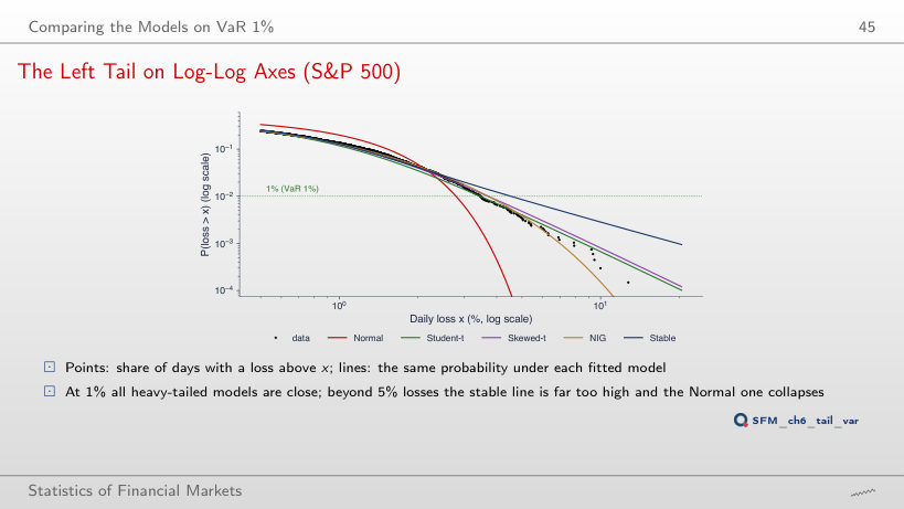
                                                        Slide 45: The Left Tail on Log-Log Axes (S&P 500)
                                                        Slide 45
                                                          Question for the room The S&P 500 has a single day with a loss above 10% (16 March 2020) in 6,714 days. How many such days does the fitted stable distribution expect in the sample?
                                                          Answer

                                                          About 19. The Normal model expects practically zero (probability 7 × 10⁻¹⁷), Student-t 4.5, NIG 1.0, GED 0.08. For losses above 5%, the data have 23 days, the stable expects 57, Student-t 27, NIG 26. The stable tail (α̂ = 1.54) is far too heavy for the S&P 500.

                                                          Counting Exceedances: the Kupiec Test
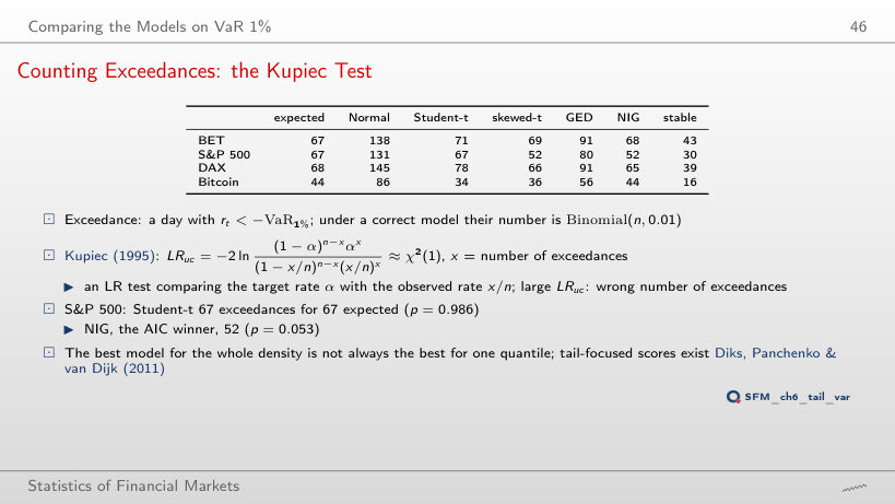
                                                          Slide 46: Counting Exceedances: the Kupiec Test
                                                          Slide 46

                                                          In-sample exceedances (Kupiec p-value in brackets)

                                                          Worked example: the Kupiec test

                                                          \[LR_{uc} = -2\ln\frac{(1-\alpha)^{n-x}\alpha^x}{(1 - x/n)^{n-x}(x/n)^x} \approx \chi^2(1)\]
                                                              Question for the room At VaR 1%, NIG (the AIC winner) has 52 exceedances for the S&P 500 against 67 expected (p = 0.053). The ▶ button goes through the levels. At VaR 2.5%, is the number of NIG exceedances rejected at 5%?
                                                              Answer

                                                              No: 151 exceedances against 167.9 expected, p = 0.18. Student-t, perfect at 1% (67 against 67), is rejected at 2.5%: 211 exceedances, p = 0.001. A model that is good for one quantile is not necessarily good for another. At VaR 0.1%, NIG has 7 exceedances against 6.7 expected, the Normal model 52.

                                                              Out of Sample: Validation and Overfitting

                                                              Out-of-Sample Results, 2020–2026
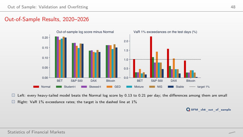
                                                              Slide 48: Out-of-Sample Results, 2020–2026
                                                              Slide 48

                                                              VaR 1% exceedances on the test days, 2020–2026 (Kupiec p-value in brackets)

                                                              Worked example: the pinball loss of the 1% quantile

                                                              \[\frac{1}{n}\sum_t \big(\alpha - \mathbf{1}\{r_t < q\}\big)(r_t - q), \qquad \alpha = 0.01\]
                                                                  Question for the room On the test period 2020–2026, which method has the lowest pinball loss of the 1% quantile for BET?
                                                                  Answer

                                                                  The Normal model (0.0475), followed by GED (0.0494); Student-t, the best by log score, has 0.0517, and NIG, the AIC winner on 2000–2019, 0.0513. The test period was calmer for BET, and the smaller Normal VaR had 17 exceedances against 16.7 expected. The right number for the wrong reason: a static model does not follow the volatility.

                                                                  Overfitting: Normal Mixtures with 1 to 6 Components
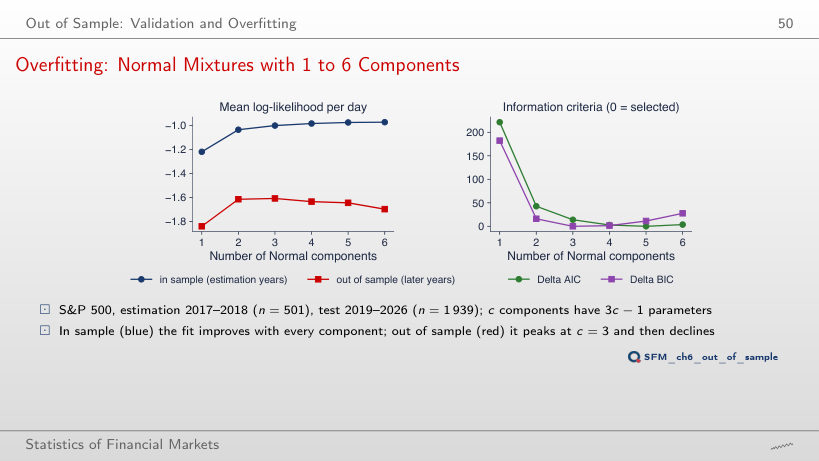
                                                                  Slide 50: Overfitting: Normal Mixtures with 1 to 6 Components
                                                                  Slide 50

                                                                  Worked example: AIC and BIC

                                                                  \[\mathrm{AIC} = -2\ell + 2k, \quad \mathrm{BIC} = -2\ell + k\ln n, \quad k = 3c - 1\]
                                                                      Question for the room With a penalty of 2 per parameter (AIC), the criterion selects c = 5 components; with ln 501 = 6.22 (BIC), c = 3. The ▶ button raises the penalty from 0 to 10. From which penalty does the choice fall to c = 3?
                                                                      Answer

                                                                      From 5.71 (in the slider's steps of 0.1, from 5.8): going from 3 to 4 components gains 2(ℓ4 − ℓ3) = 17.14 for 3 extra parameters, i.e. 5.71 per parameter. Below 0.8, c = 6 is selected, between 0.8 and 3 c = 5, between 3 and 5.71 c = 4. Out of sample the best is c = 3 (−1.608 per day), while c = 6 gives −1.698.

                                                                      Rolling VaR 1%: Refit Every Month
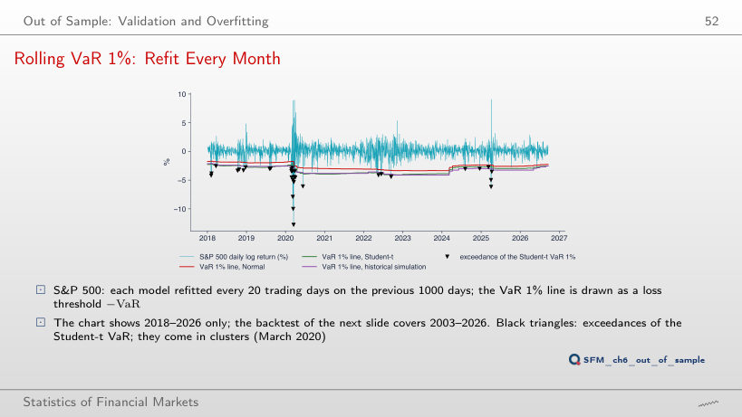
                                                                      Slide 52: Rolling VaR 1%: Refit Every Month
                                                                      Slide 52

                                                                      Exceedances per year

                                                                      Backtest over the whole test period

                                                                      Worked example: the Christoffersen independence test (extra run)

                                                                      \[LR_{ind} = -2\ln\frac{(1-\hat\pi)^{n_{00}+n_{10}}\,\hat\pi^{\,n_{01}+n_{11}}}{(1-\hat\pi_{01})^{n_{00}}\hat\pi_{01}^{\,n_{01}}(1-\hat\pi_{11})^{n_{10}}\hat\pi_{11}^{\,n_{11}}} \approx \chi^2(1)\]
                                                                          Question for the room S&P 500, rolling Student-t VaR 1%: 89 exceedances in 5,714 days (1.56%), Kupiec p < 0.001. Are the exceedances independent over time? (the Christoffersen test, extra run)
                                                                          Answer

                                                                          No: LRind = 19.81, p < 0.001. After a day with an exceedance, another follows in 10.1% of the cases (9 of 89), against 1.4% after a day without. The exceedances pile up in August 2007, September–November 2008 (6, 9 and 6) and March 2020 (9). For BET, historical simulation passes the Kupiec test (p = 0.066) but not the independence test (p = 0.014).

                                                                          The VaR Reliability Plot (SFEVaRqqplot)
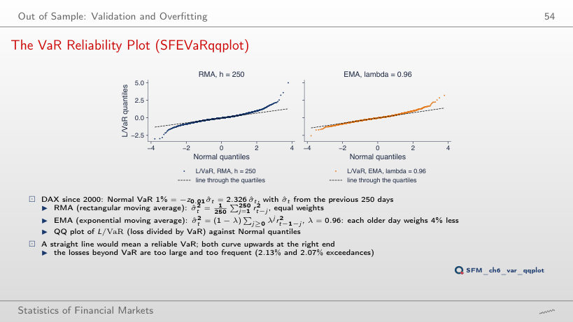
                                                                          Slide 54: The VaR Reliability Plot (SFEVaRqqplot)
                                                                          Slide 54
                                                                            Question for the room With λ = 0.96, the Normal VaR with EMA volatility is exceeded on 2.07% of the DAX days. The ▶ button moves λ from 0.90 to 0.99. Does the rate approach 1% for any λ?
                                                                            Answer

                                                                            No: the rate stays between 1.96% (λ = 0.97) and 2.40% (λ = 0.99). The EMA volatility adapts, but the Normal quantile z0.01 = −2.326 remains too small for the standardised returns, whose tails are heavier than those of the Normal distribution: the right end of the QQ plot bends upwards for every λ. RMA with h = 250 has 2.13%; with h = 125, 2.21%.

                                                                            Model Uncertainty

                                                                            Uncertainty of the Model Ranking
                                                                            Slide 55: Uncertainty of the Model Ranking
                                                                            Slide 55

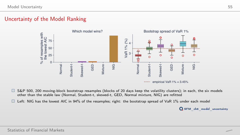
                                                                            Moving-block bootstrap resamples, S&P 500

                                                                              Question for the room With all 200 resamples, NIG has the lowest AIC in 93.5% of them. The ▶ button raises B from 20 to 200. What share do the first 20 resamples give?
                                                                              Answer

                                                                              100%: NIG wins all of the first 20. With B = 40, 95%; with B = 100, 95%; with B = 200, 93.5% (GED 3.5%, skewed-t 3%). A small number of resamples overstates the certainty about the winner. The 90% intervals of VaR 1% (Student-t [3.14, 3.87]%, NIG [3.34, 4.18]%) overlap: the uncertainty between models is comparable to the uncertainty within a model.

                                                                              Model Averaging and Model Risk
                                                                              Slide 57: Model Averaging and Model Risk
                                                                              Slide 57

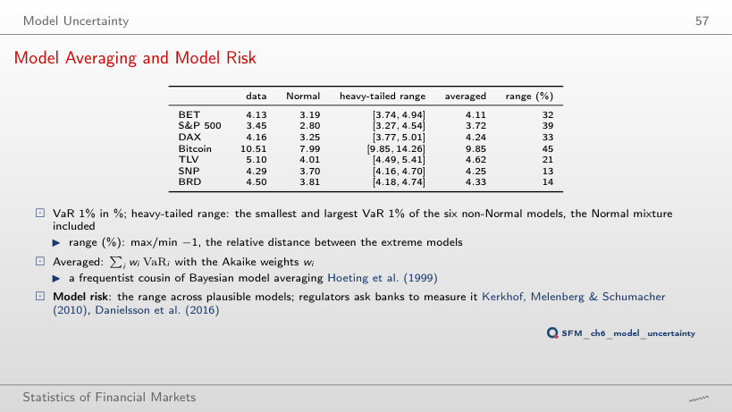
                                                                              VaR (%) of the data, of the models and averaged

                                                                              Worked example: the averaged VaR

                                                                              \[\mathrm{VaR}^{avg}_\alpha = \sum_i w_i\,\mathrm{VaR}_{\alpha,i}, \qquad \text{range} = \frac{\max_i \mathrm{VaR}_i}{\min_i \mathrm{VaR}_i} - 1\]
                                                                                  Question for the room For TLV, the VaR 1% range of the heavy-tailed models is [4.49, 5.41]. The stable distribution, with the heaviest tails, gives 4.92%. Which model gives the upper end, 5.41%?
                                                                                  Answer

                                                                                  The Normal mixture (the mixture column of the lecture's VaR table), one of the six non-Normal models. Without it, the TLV range becomes [4.49, 4.92], 10% instead of 21%. The same holds for SNP (4.70%) and BRD (4.74%). For the indices and Bitcoin, the upper end comes from the stable distribution.

                                                                                  Daily log returns, in %: BET, S&P 500 and DAX from January 2000, Bitcoin from September 2014 (7 days a week), Banca Transilvania (TLV), OMV Petrom (SNP) and BRD from 2010, from the adjusted price, to 18 September 2026; the two erroneous TLV days of May 2016 are removed. Monthly DAX: first trading day of each month (SFESumm). EODHD closing prices. The fitted parameters, log-likelihoods, model quantiles, rolling VaR and bootstrap resamples are those of the lecture (the same code and the same generator seed); the summary statistics, empirical VaR and ES, exceedances, Kupiec tests, pinball losses and the SFEVaRqqplot chart are recomputed in the browser from the same returns. VaR levels other than 1%, the profile of ν for the other series, the Christoffersen test and the BIC weights are extra runs of the same code.