

Statistics of Financial Markets

Chapter 7 · Efficient Markets, Random Walk and Variance-Ratio Tests

The slide of the lecture is on the left, the same figure or table on the right, computed in the browser from the same data. The ▶ button moves the parameter step by step; the tables and worked examples are recomputed with it. Abbreviations: ACF (autocorrelation function), VR (variance ratio), ADF (augmented Dickey–Fuller), PP (Phillips–Perron), KPSS (Kwiatkowski–Phillips–Schmidt–Shin), LB (Ljung–Box), CD (Chow–Denning), OLS (ordinary least squares), GARCH (generalised autoregressive conditional heteroskedasticity).

Predictability of Prices · Random Walk Hypotheses · White Noise and the Autocorrelation Function · Testing for Autocorrelation · Unit Roots: Prices against Returns · The Variance-Ratio Test · Efficiency across Markets and over Time · Semi-Strong Form, Strong Form and Anomalies

Predictability of Prices

Question for the Room: Which Path Is the S&P 500?
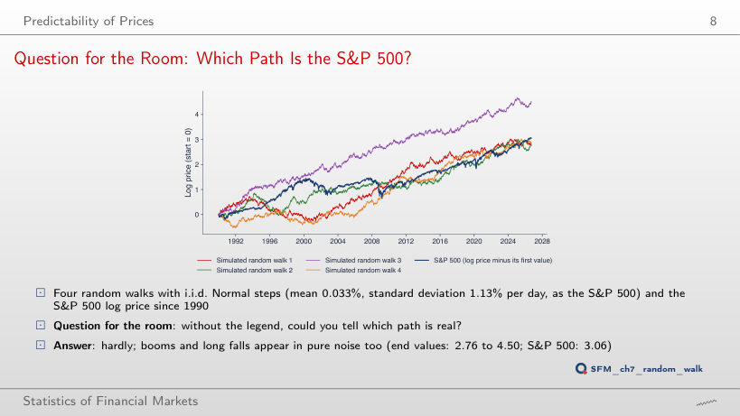
Slide 8: Question for the Room: Which Path Is the S&P 500?
Slide 8
    Question for the room Four random walks with i.i.d. Normal steps (the mean and standard deviation of the S&P 500) and the S&P 500 itself. The ▶ button draws the paths year by year, from 1991 to 2026. At the end of 2008, how many of the four random walks are above the S&P 500?
    Answer

    Three. At the end of 2008 the S&P 500 is at 0.91 (log price minus its first value), the simulated walks at 1.12, 1.24, 2.69 and 0.65. In September 2026 only one (4.50) is above the S&P 500 (3.06). The falls of 2000–2002 and 2008 have the size of episodes that pure noise also produces: a single path does not separate the S&P 500 from a random walk.

    Yesterday's Return and Today's Return
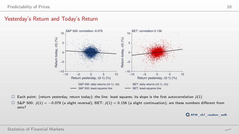
    Slide 10: Yesterday's Return and Today's Return
    Slide 10
      Question for the room The correlation between today's and yesterday's return is −0.079 for the S&P 500 and 0.156 for the BET. The ▶ button moves the lag from 1 to 10. What is the BET correlation at lag 2, between today's return and that of two days ago?
      Answer

      0.033, almost five times smaller; at lag 3 it is −0.008, at lag 5 0.031, at lag 10 0.004. For the S&P 500 the lag-2 correlation is −0.004. Almost all the dependence of the BET returns sits at lag 1, as thin trading produces: news enters the index over two days.

      Random Walk Hypotheses

      Worked Example: Risk as a Function of the Horizon
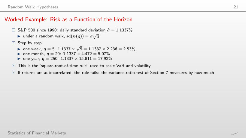
      Slide 21: Worked Example: Risk as a Function of the Horizon
      Slide 21

      Standard deviation of q-day returns: the square-root rule and the data

      Worked example: the square-root-of-time rule

      \[\mathrm{sd}\big(r_t(q)\big) = \sigma\sqrt{q}, \qquad \frac{\mathrm{sd}\big(r_t(q)\big)}{\sigma\sqrt{q}} \approx \sqrt{\mathrm{VR}(q)}\]
          Question for the room The square-root-of-time rule gives the S&P 500 a 250-day standard deviation of 1.1337% × √250 = 17.92%. Is the standard deviation of 250-day returns, computed directly from the overlapping sums, larger or smaller?
          Answer

          Smaller: 15.66%, that is 0.874 of the rule's value. The daily S&P 500 returns are slightly negatively autocorrelated (ρ̂(1) = −0.079, VR(250) = 0.785), so daily moves partly cancel over time. The BET, with ρ̂(1) = 0.156, shows the opposite: 35.91% against 23.38% (1.54 times). The rule assumes uncorrelated returns; scaling VaR or volatility by √q inherits this assumption.

          White Noise and the Autocorrelation Function

          Gaussian White Noise and Its Sample ACF
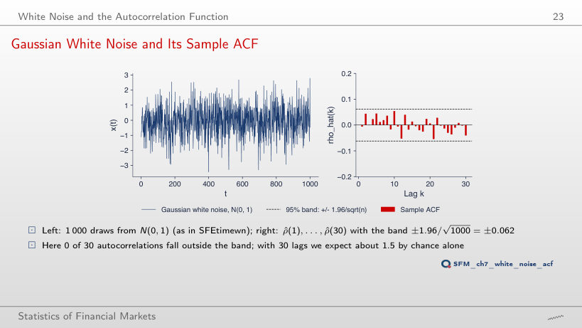
          Slide 23: Gaussian White Noise and Its Sample ACF
          Slide 23
            Question for the room For n = 1,000 draws the 95% band is ±0.062 and 0 of 30 sample autocorrelations lie outside it. The ▶ button uses only the first n draws, from 100 to 1,000. For n = 100, with the band ±0.196, how many autocorrelations lie outside the band?
            Answer

            One: the largest in absolute value is 0.223. With 30 lags we expect 1.5 exceedances by chance alone, at any n: the band widens as 1/√n, and the sample autocorrelations of white noise grow at the same rate. At n = 400 one lies outside as well, at the other values of n none.

            Theoretical and Sample ACF of Six Processes
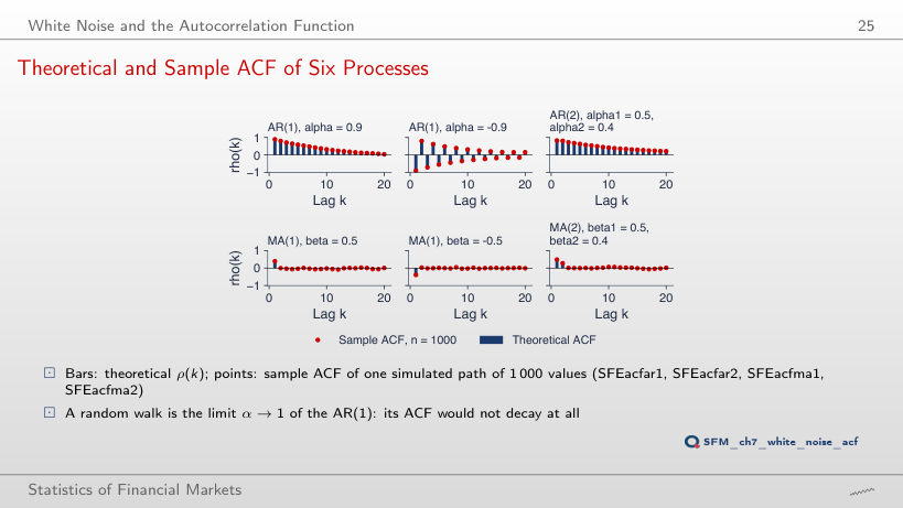
            Slide 25: Theoretical and Sample ACF of Six Processes
            Slide 25
              Question for the room The red points are the sample ACF of one simulated path of 1,000 values. The ▶ button uses only the first n values, from 50 to 1,000. For the AR(1) with α = 0.9, how far does the sample ACF get from the theoretical one at n = 50?
              Answer

              Up to 0.40 (the largest deviation over lags 1–20), against 0.08 at n = 1,000. The white-noise band for n = 50 is ±0.28 (1/√50 = 0.14), but the deviation is larger, because the variance of ρ̂(k) of a persistent process exceeds 1/T. For the MA(2), the largest deviation is 0.19 at n = 50 and 0.06 at n = 1,000.

              The ACF of Daily Returns
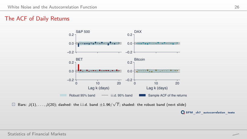
              Slide 26: The ACF of Daily Returns
              Slide 26

              Worked example: the robust band of the ACF

              \[\hat\delta(k) = \frac{T\sum_t e_t^2 e_{t-k}^2}{\big(\sum_t e_t^2\big)^2}, \qquad \pm 1.96\sqrt{\hat\delta(k)/T}, \qquad e_t = r_t - \bar r\]
                  Question for the room From 1990, the S&P 500 has 9 autocorrelations (of 20) outside the i.i.d. band and 3 outside the robust band. The ▶ button moves the start of the sample towards 2022. What happens to the S&P 500 ρ̂(1) on the sample that starts in 2016?
                  Answer

                  It becomes more negative: −0.142, against −0.079 from 1990, with 13 lags outside the i.i.d. band and 7 outside the robust band. On the sample that starts in 2022, ρ̂(1) is only −0.015. On rolling windows (section "Efficiency across Markets and over Time") the S&P 500 reversals are strongest in crises: the sample from 2016 includes 2020, the one from 2022 does not.

                  Autocorrelation of Returns and of Absolute Returns
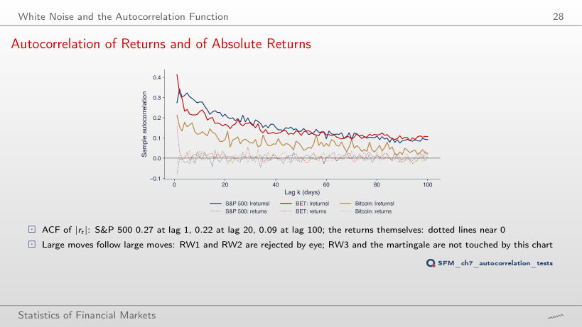
                  Slide 28: Autocorrelation of Returns and of Absolute Returns
                  Slide 28
                    Question for the room The ACF of |rt| for the S&P 500 is 0.27 at lag 1, 0.22 at lag 20 and 0.09 at lag 100. The ▶ button raises the power d in |rt|d up to 2 (squared returns). What happens to the lag-100 autocorrelation when d goes from 1 to 2?
                    Answer

                    It falls: 0.039 for d = 2, against 0.092 for d = 1; at lag 1 it rises slightly (0.311 against 0.275). High powers give weight to a few extreme days, and their autocorrelation dies out faster. For every d the size of the returns stays correlated, so RW1 and RW2 are rejected.

                    Testing for Autocorrelation

                    Worked Example: Ljung–Box Step by Step
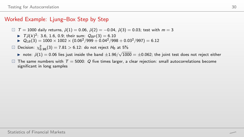
                    Slide 30: Worked Example: Ljung–Box Step by Step
                    Slide 30

                    Worked example: Box–Pierce and Ljung–Box

                    \[Q_{BP}(m) = T\sum_{k=1}^{m}\hat\rho(k)^2, \qquad Q_{LB}(m) = T(T+2)\sum_{k=1}^{m}\frac{\hat\rho(k)^2}{T-k} \approx \chi^2(m)\]
                        Question for the room With T = 1,000 and the autocorrelations 0.06, −0.04 and 0.03, QLB(3) = 6.12 < 7.81: we do not reject. The ▶ button raises T up to 5,000, with the same autocorrelations. From which T does the test reject at 5%?
                        Answer

                        From T = 1,500 (in steps of 500): QLB(3) = 9.17 > 7.81, p = 0.027. The statistic grows almost in proportion to T (30.52 at T = 5,000); the exact threshold is around T = 1,280. The autocorrelations are the same; with more data they are estimated more precisely and separate from zero. In long samples, small autocorrelations become significant without being larger.

                        Autocorrelation Tests on Real Data
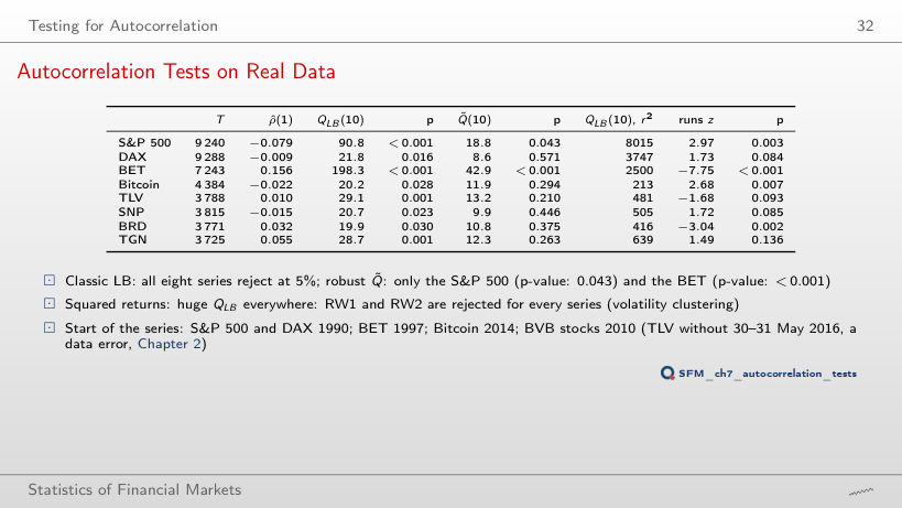
                        Slide 32: Autocorrelation Tests on Real Data
                        Slide 32

                        Tests on the daily returns (p-value below 0.05 in red)

                        Worked example: QLB and Q̃ on real data

                        \[\tilde Q(m) = \sum_{k=1}^{m}\frac{T\hat\rho(k)^2}{\hat\delta(k)} \approx \chi^2(m)\]
                            Question for the room With m = 10 lags, the classical QLB rejects for all eight series, the robust Q̃ only for the S&P 500 and the BET. The ▶ button raises m up to 30. With m = 30, for which series does the robust Q̃ reject?
                            Answer

                            Only for the BET (Q̃(30) = 67.9 > 43.77). The S&P 500 no longer rejects: Q̃(30) = 39.7, because its lag-1 autocorrelation is diluted among 29 nearly zero lags; the slide says the same: a larger m dilutes a short-lived effect. The classical QLB rejects at m = 30 for five series, with a χ² distribution that ignores volatility clustering.

                            The Runs Test
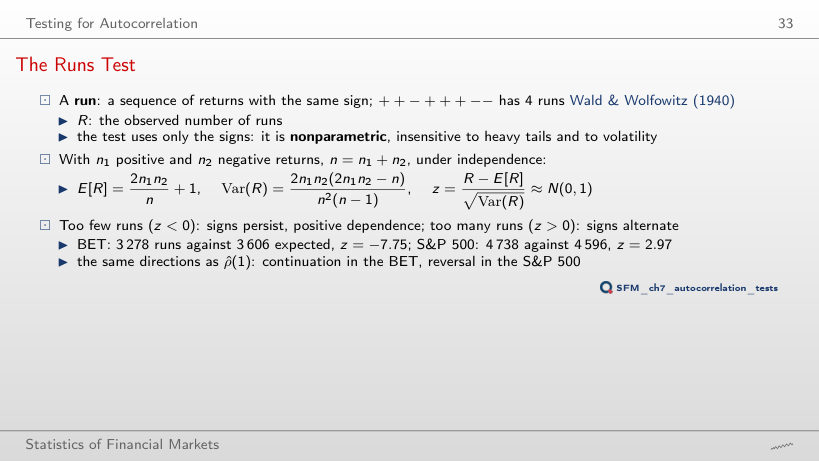
                            Slide 33: The Runs Test
                            Slide 33

                            Worked example: the runs test

                            \[E[R] = \frac{2n_1n_2}{n} + 1, \quad \mathrm{Var}(R) = \frac{2n_1n_2(2n_1n_2 - n)}{n^2(n-1)}, \quad z = \frac{R - E[R]}{\sqrt{\mathrm{Var}(R)}}\]
                                Question for the room Over the whole sample, the BET has 3,278 runs against 3,606 expected (z = −7.75), the S&P 500 4,738 against 4,596 (z = 2.97). The ▶ button moves the start of the sample towards 2022. On the sample that starts in 2022, does either of these two rejections remain?
                                Answer

                                Only the BET one, much weaker: z = −2.03, against 0.06 for the S&P 500. The BET signs persist in recent years too, but much less than over the whole sample; for the S&P 500 the alternation of signs disappears. From 2022, BRD has z = −3.79.

                                Unit Roots: Prices against Returns

                                Practical Consequence: Spurious Regression
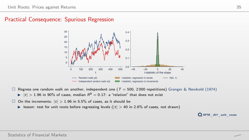
                                Slide 35: Practical Consequence: Spurious Regression
                                Slide 35
                                  Question for the room With T = 500, regressing one random walk on another, independent one gives |t| > 1.96 in 90% of the 2,000 replications. The ▶ button raises T to 1,000 and 2,000 (T ≠ 500: extra runs of the lecture code). Does the share of rejections approach 5% as T grows?
                                  Answer

                                  No, it rises: 92.7% at T = 1,000 and 94.5% at T = 2,000 (77.3% at T = 100); |t| > 40 occurs in 21.6% of the regressions at T = 2,000. In the regression in levels the t-statistic grows with T, so more data make the spurious relation more convincing. The median R² stays between 0.16 and 0.18. In increments, the share stays between 5.1% and 6.0% for every T.

                                  The Augmented Test and a Worked Example
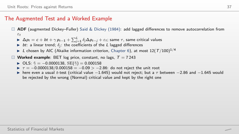
                                  Slide 37: The Augmented Test and a Worked Example
                                  Slide 37

                                  Worked example: the Dickey–Fuller regression

                                  \[\Delta p_t = c + bt + \gamma\, p_{t-1} + \sum_{j=1}^{L}\delta_j\Delta p_{t-j} + \varepsilon_t, \qquad \tau = \frac{\hat\gamma}{\mathrm{SE}(\hat\gamma)}\]
                                      Question for the room For the BET log price, the Dickey–Fuller regression with a constant and no lags gives τ = −0.09. The ▶ button runs through the eight series; the curve shows τ for L = 0–40 lags of the differences. Does the test with a constant reject the unit root for any series, at any L?
                                      Answer

                                      No. The lowest τ with a constant is −1.41 (Bitcoin, L = 20), far from −2.86; for TLV, SNP, BRD and TGN τ is even positive. Prices grow over time, so the right specification has a constant and a trend: with it, TLV falls below −3.41 at 12 of the 16 values of L (τ = −3.46 at L = 20, the order chosen by AIC).

                                      The BET: Log Price and Returns
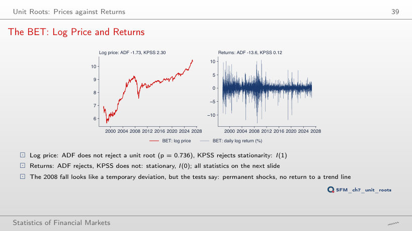
                                      Slide 39: The BET: Log Price and Returns
                                      Slide 39
                                        Question for the room For the BET, ADF on the log price is −1.73 (p = 0.736) and KPSS 2.30: the price is I(1). The ▶ button runs through the eight series. For which series do the tests on the log price not give the conclusion I(1)?
                                        Answer

                                        TLV: ADF = −3.46 < −3.41 (p = 0.044) rejects the unit root, and KPSS = 0.57 > 0.146 rejects trend stationarity. The tests contradict each other: an inconclusive case, not evidence of reversion to a trend. For the other seven series ADF does not reject and KPSS rejects. The returns are I(0) for all eight.

                                        Unit-Root Tests on Prices and Returns
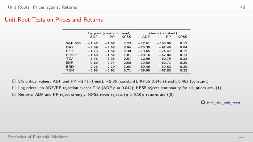
                                        Slide 40: Unit-Root Tests on Prices and Returns
                                        Slide 40

                                        Test statistics (in red: rejection at 5%)

                                        Worked example: the KPSS statistic on the log price

                                        \[\mathrm{KPSS} = \frac{\sum_{t=1}^{T} S_t^2}{T^2\hat\lambda^2}, \quad S_t = \sum_{s \le t} e_s, \quad \hat\lambda^2 = \hat\gamma(0) + 2\sum_{j=1}^{l}\Big(1 - \frac{j}{l+1}\Big)\hat\gamma(j)\]
                                            Question for the room With the bandwidth of the lecture (l = 38 for the S&P 500), KPSS rejects stationarity of the prices for all eight series; KPSS on the S&P 500 price is 2.23. The ▶ button changes the bandwidth l of the long-run variance, starting with l = 0. What is KPSS for the S&P 500 price at l = 0?
                                            Answer

                                            86.0. An integrated price has large positive autocovariances; without them, λ̂² is just the variance of the residuals and understates the long-run variance by a factor of several dozen. The statistic falls as l grows, but at l = 80 it is still 1.09 > 0.146. On returns, KPSS stays below 0.463 for every l: the conclusion I(1) for prices and I(0) for returns does not depend on the bandwidth.

                                            The Variance-Ratio Test

                                            Worked Example: VR from the ACF of the S&P 500
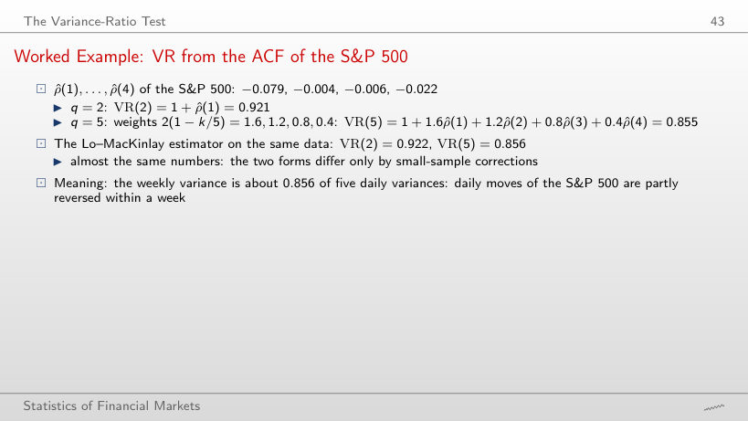
                                            Slide 43: Worked Example: VR from the ACF of the S&P 500
                                            Slide 43

                                            Worked example: VR from the ACF

                                            \[\mathrm{VR}(q) = 1 + 2\sum_{k=1}^{q-1}\Big(1 - \frac{k}{q}\Big)\hat\rho(k)\]
                                                Question for the room From the ACF of the S&P 500, VR(5) = 1 + 1.6ρ̂(1) + 1.2ρ̂(2) + 0.8ρ̂(3) + 0.4ρ̂(4) = 0.855, and the Lo–MacKinlay estimator gives 0.856. The ▶ button raises q up to 20. How much do the two values differ at q = 20?
                                                Answer

                                                Very little: 0.768 from the ACF and 0.767 with the Lo–MacKinlay estimator, a difference of 0.0005. For the BET at q = 20: 1.514 and 1.517. The two forms differ only by small-sample corrections, which matter little with T = 9,240 and q = 20.

                                                Lo and MacKinlay (1988): Estimator and Tests
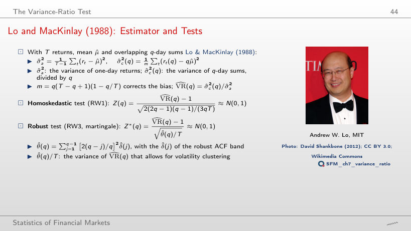
                                                Slide 44: Lo and MacKinlay (1988): Estimator and Tests
                                                Slide 44

                                                Worked example: Z(q) and Z*(q)

                                                \[Z(q) = \frac{\widehat{\mathrm{VR}}(q) - 1}{\sqrt{2(2q-1)(q-1)/(3qT)}}, \qquad Z^*(q) = \frac{\widehat{\mathrm{VR}}(q) - 1}{\sqrt{\hat\theta(q)/T}}, \qquad \hat\theta(q) = \sum_{j=1}^{q-1}\Big[\frac{2(q-j)}{q}\Big]^2\hat\delta(j)\]
                                                    Question for the room For the S&P 500 at q = 2, Z(2) = −7.54 and Z*(2) = −3.37: the homoskedastic statistic is 2.24 times larger in absolute value. The ▶ button raises q up to 40. At q = 40, does Z* still reject the random walk for the S&P 500?
                                                    Answer

                                                    No: Z*(40) = −1.81, although Z(40) = −3.70 still rejects. At q = 40, Z* rejects only for the BET. The ratio Z/Z* stays between 2.0 and 2.3 at all horizons: volatility clustering doubles the standard error of the estimated VR(q), and Z(q) ignores it.

                                                    The Need for a Robust Test: a Monte Carlo Study
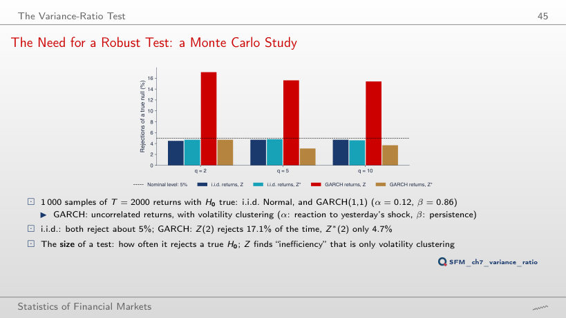
                                                    Slide 45: The Need for a Robust Test: a Monte Carlo Study
                                                    Slide 45
                                                      Question for the room Under a GARCH(1,1) martingale with α = 0.12 and β = 0.86, Z(2) rejects the true null in 17.1% of the cases, Z*(2) in 4.7%. The ▶ button moves the reaction α from 0 to 0.12, with β = 0.86 fixed (α ≠ 0.12: extra runs of the lecture simulation). At α = 0.09, how often does Z(2) reject?
                                                      Answer

                                                      In 9.0% of the cases; at α = 0.06 in 6.2%, at α = 0 in 4.8%. The distortion grows fast as α + β approaches 1 (0.95 at α = 0.09, 0.98 at α = 0.12), because volatility becomes very persistent. Z*(2) stays between 4.3% and 4.9% for every α.

                                                      Variance Ratios for Horizons of 2 to 40 Days
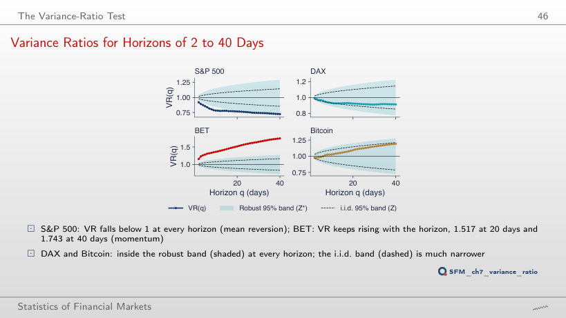
                                                      Slide 46: Variance Ratios for Horizons of 2 to 40 Days
                                                      Slide 46
                                                        Question for the room From 1990, VR(40) is 0.724 for the S&P 500 and 1.743 for the BET, and Z* rejects for the BET at all 39 horizons. The ▶ button moves the start of the sample towards 2022. On the sample that starts in 2010, does Z* still reject the BET momentum at any horizon q = 2, …, 40?
                                                        Answer

                                                        No: the BET VR(40) falls to 1.193 and no Z*(q) exceeds 1.96. The BET momentum comes from the early years (1997–2006, ρ̂(1) = 0.270). From 2010 the S&P 500 rejects at a single horizon of 39, with VR(40) = 0.663, below the value from 1990: the mean reversion remains, but the robust band widens with the shorter sample.

                                                        Variance Ratios and Robust Tests
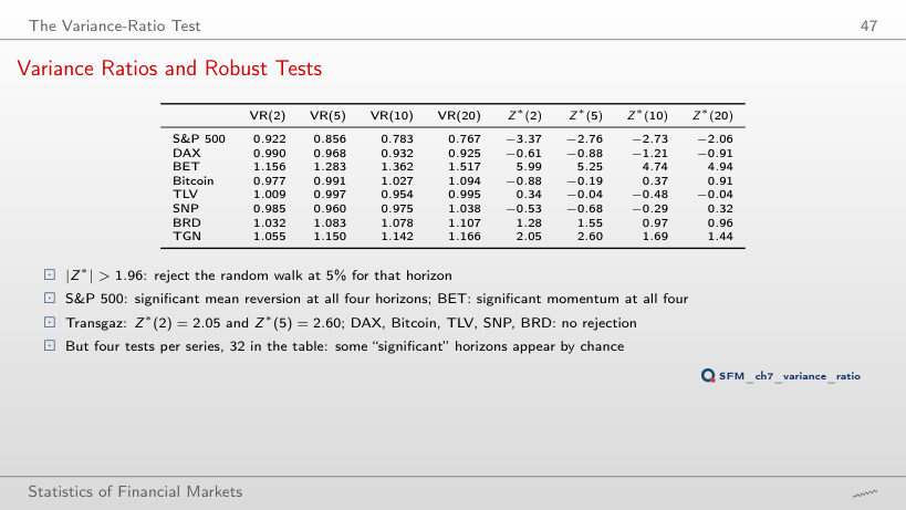
                                                        Slide 47: Variance Ratios and Robust Tests
                                                        Slide 47
                                                          Question for the room Over the whole sample, 10 of the 32 Z* statistics in the table exceed 1.96 in absolute value. The ▶ button moves the start of the sample towards 2022. On the sample that starts in 2010, how many remain?
                                                          Answer

                                                          Three: the S&P 500 at q = 2 and Transgaz at q = 2 and 5 (for Transgaz the sample starts in 2010 anyway). The BET no longer rejects at any horizon. With the homoskedastic Z there would be 13, because Z ignores volatility clustering. With 32 independent tests at 5% we would expect 1.6 false rejections on average.

                                                          Joint and Automatic Tests on Real Data
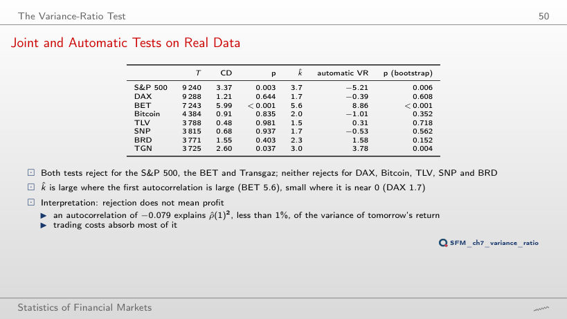
                                                          Slide 50: Joint and Automatic Tests on Real Data
                                                          Slide 50

                                                          Worked example: the Chow–Denning test

                                                          \[\mathrm{CD} = \max_i |Z^*(q_i)|, \qquad P(\mathrm{CD} \le c) = \big(2\Phi(c) - 1\big)^m\]

                                                            Worked example: the automatic VR test

                                                            \[\hat k = 1.3221\,(\hat a_2 T)^{1/5}, \quad \hat a_2 = \frac{4\hat\rho^2}{(1-\hat\rho)^4}, \qquad \frac{\sqrt{T/\hat k}\,\big(\mathrm{VR}(\hat k) - 1\big)}{\sqrt 2} \approx N(0, 1)\]
                                                                Question for the room With the horizons 2, 5, 10, 20 (m = 4), the 5% Chow–Denning critical value is 2.49 and the test rejects for the S&P 500, the BET and Transgaz. The ▶ button changes the set of horizons. With all horizons 2, …, 20 (m = 19), which series still reject?
                                                                Answer

                                                                The S&P 500 and the BET. The critical value rises to 3.00, and Transgaz, with CD = 2.77, no longer exceeds it. More horizons mean more chances of a false rejection, hence a higher threshold; CD rises only if the added horizons have a larger |Z*|.

                                                                Efficiency across Markets and over Time

                                                                Sixteen Markets over the Last Ten Years
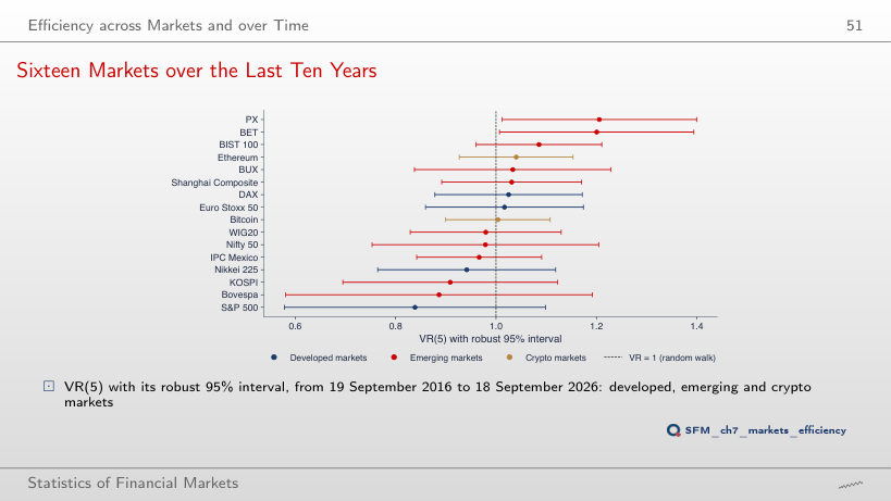
                                                                Slide 51: Sixteen Markets over the Last Ten Years
                                                                Slide 51
                                                                  Question for the room At q = 5, only the robust 95% intervals of PX (Z* = 2.08) and the BET (Z* = 2.03) exclude the value 1. The ▶ button raises the horizon q up to 20. At q = 20, which market excludes the value 1?
                                                                  Answer

                                                                  Only Ethereum (VR(20) = 1.29, Z* = 2.45); PX and the BET return inside the interval. At q = 2 it is the S&P 500 (VR(2) = 0.86, Z* = −2.33). Each horizon shows a different market: with 16 markets and many horizons, some intervals exclude 1 by chance, and the Chow–Denning test on four horizons rejects for no market.

                                                                  Rolling Variance Ratios
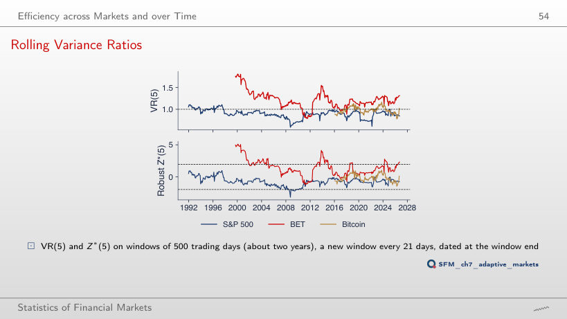
                                                                  Slide 54: Rolling Variance Ratios
                                                                  Slide 54
                                                                    Question for the room On 500-day windows, 29% of the BET windows and 4% of the S&P 500 windows reject at 5%. The ▶ button lengthens the window to 750, 1,000 and 1,500 days. What happens to the share of rejecting S&P 500 windows at 1,500 days?
                                                                    Answer

                                                                    It rises to 20%, all with VR < 1. A long window estimates the same small negative autocorrelation more precisely, so it separates it from zero more easily; at 250 days the share is 1.6%. Consecutive windows share 1,479 of 1,500 days, so the share describes the data and is not a test.

                                                                    Three Sub-Periods per Market
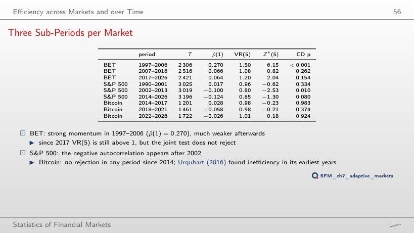
                                                                    Slide 56: Three Sub-Periods per Market
                                                                    Slide 56
                                                                      Question for the room At q = 5, the S&P 500 rejects in 2002–2013 (Z*(5) = −2.53). The ▶ button raises q to 10 and 20. At q = 20, does any S&P 500 sub-period still reject?
                                                                      Answer

                                                                      None: Z*(20) = −1.33, −1.54 and −0.91, although VR(20) = 0.72 in 2002–2013, further from 1 than VR(5) = 0.80. The variance of VR(q) grows with q, and with about 3,000 days per sub-period the robust interval becomes wide. Only the BET 1997–2006 rejects at q = 20 (Z*(20) = 5.14).

                                                                      Semi-Strong Form, Strong Form and Anomalies

                                                                      Day-of-Week Returns: S&P 500 and BET
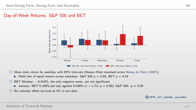
                                                                      Slide 60: Day-of-Week Returns: S&P 500 and BET
                                                                      Slide 60

                                                                      Worked example: the January effect

                                                                      \[r_t = a + b\,\mathbf{1}\{\text{January}\}_t + u_t, \qquad t = \frac{\hat b}{\mathrm{SE}_{NW}(\hat b)}\]
                                                                          Question for the room The Wald test of equal means across the days of the week gives p = 0.69 for the S&P 500 and 0.24 for the BET (Newey–West standard errors with 5 lags). The ▶ button moves the start of the sample towards 2022. Does the BET p-value fall below 0.05 for any start?
                                                                          Answer

                                                                          No: the lowest is 0.088, for the sample that starts in 2016; the S&P 500 stays above 0.62. Trying 17 different starts is itself a repeated search of the data: even a p below 0.05 at one of them would not be evidence of a day-of-week effect.

                                                                          Daily log returns, in %: S&P 500 and DAX from January 1990, BET from September 1997, Bitcoin from September 2014 (7 days a week), Banca Transilvania (TLV), OMV Petrom (SNP), BRD and Transgaz (TGN) from 2010, from the adjusted price, to 18 September 2026; the two erroneous TLV days of May 2016 are removed. Cross-market comparison: 16 indices and cryptocurrencies, 19 September 2016 to 18 September 2026. EODHD closing prices. The simulated random walks, the white noise, the ARMA paths, the spurious regressions, the size simulation of Z and Z*, the ADF lag orders chosen by AIC and the wild-bootstrap p-values are those of the lecture (the same code and the same generator seed); the autocorrelations, the portmanteau and runs tests, the Dickey–Fuller regressions, PP, KPSS, the variance ratios, the Chow–Denning test, the automatic VR test, the rolling windows, the sub-periods and the calendar regressions are recomputed in the browser from the same data. Other lengths T of the spurious regression, other values α of the GARCH simulation, and other bandwidths, lags, horizons and sample starts are extra runs of the same code.