

Time Series Analysis

Chapter 10 · State Space Models, the Kalman Filter and Markov Switching

The slide of the lecture is on the left, the same figure or table on the right, computed in the browser from the same data. The ▶ button moves the parameter step by step; the “Worked example” boxes redo the calculation with the numbers of the chapter.

The state space form · The Kalman filter · Smoothing, likelihood and missing data · Trend, cycle and common factors · Markov switching

The state space form

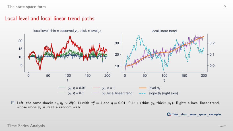
Local level and local linear trend paths
Slide 9: Local level and local linear trend paths
Slide 9
    Question for the room With T = 200, which path has the lag-1 autocorrelation of Δyt closest to −0.5?
    Answer

    The one with q = 0.01: −0.51 (theory −1/2.01 = −0.50); for q = 1 the autocorrelation is −0.28 (theory −1/3). When the noise dominates, Δyt ≈ εt − εt−1, an MA(1) with ρ(1) = −1/2; the first difference of a random walk without noise would be uncorrelated.

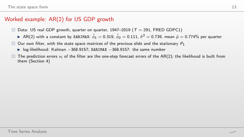
    Worked example: AR(2) for US GDP growth
    Slide 13: Worked example: AR(2) for US GDP growth
    Slide 13

    Worked example

    \[\mathrm{vec}(P_1)=(I-T\otimes T)^{-1}\mathrm{vec}(Q),\quad v_t=y_t-\hat\mu-Za_t,\quad F_t=ZP_tZ^{\prime},\quad \log L=-\tfrac12\sum_t\Big(\log 2\pi+\log F_t+\frac{v_t^2}{F_t}\Big)\]
        Question for the room What is F1, the variance of the first prediction error of the AR(2) filter?
        Answer

        0.858 = γ(0), the stationary variance of the AR(2), the (1,1) element of P1. F2 = 0.748, and from t = 3 on, with two lags known, Ft = σ̂² = 0.739. A stationary model needs no diffuse start.

        The Kalman filter

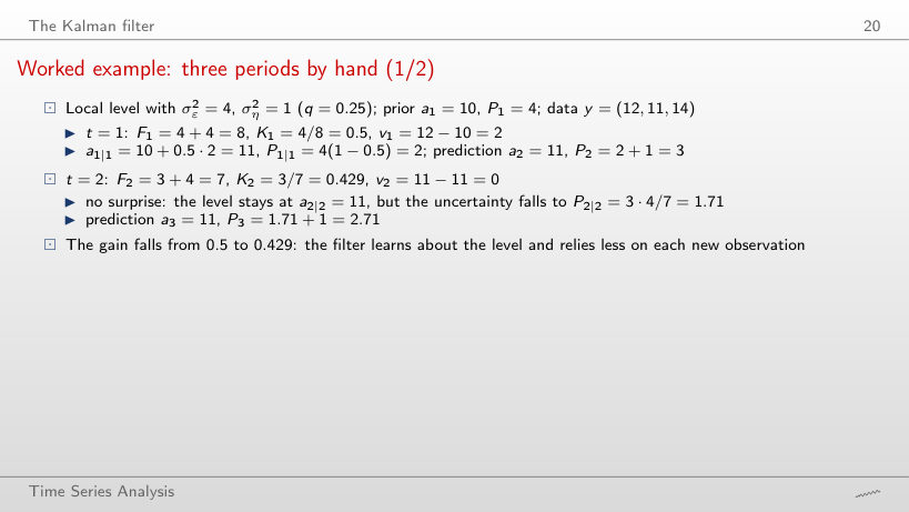
        Worked example: three periods by hand (1/2)
        Slide 20: Worked example: three periods by hand (1/2)
        Slide 20

        Worked example

        \[F_t=P_t+\sigma^2_\varepsilon,\quad K_t=\frac{P_t}{F_t},\quad a_{t|t}=a_t+K_tv_t,\quad P_{t|t}=P_t(1-K_t),\quad P_{t+1}=P_{t|t}+\sigma^2_\eta\]
            Question for the room ▶ raises σ²ε. At σ²ε = 8 (with P1 = 4), what is K1?
            Answer

            K1 = 4/(4 + 8) = 0.333: with noisier measurements the filter relies less on the observation, and the filtered level stays closer to the prediction (a1|1 = 10.67 instead of 11).

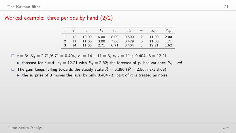
            Worked example: three periods by hand (2/2)
            Slide 21: Worked example: three periods by hand (2/2)
            Slide 21
              Question for the room Set y3 = 18 (the surprise becomes 7 instead of 3). How far does the level move at t = 3?
              Answer

              By K3v3 = 0.404·7 = 2.83, to a3|3 = 13.83. The gain K3 = 2.71/6.71 = 0.404 does not depend on the data, only on P3 and σ²ε: a larger surprise moves the level proportionally, not to the observation.

              Steady state and exponential smoothing
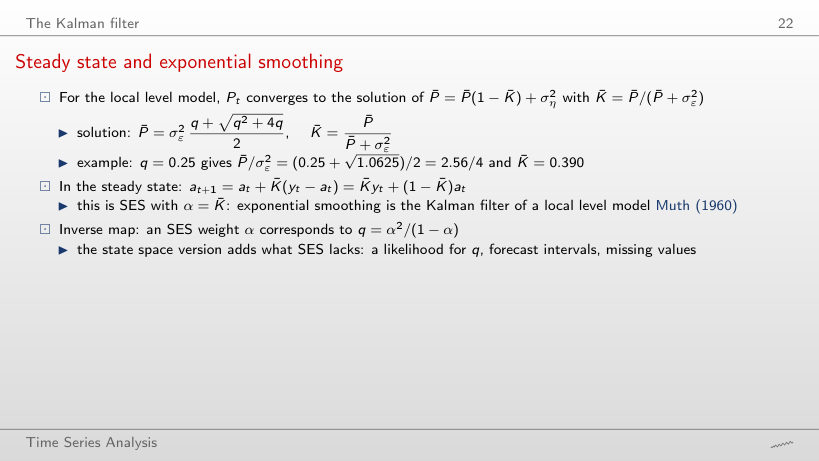
              Slide 22: Steady state and exponential smoothing
              Slide 22

              Worked example

              \[\bar P=\sigma^2_\varepsilon\,\frac{q+\sqrt{q^2+4q}}{2},\qquad \bar K=\frac{\bar P}{\bar P+\sigma^2_\varepsilon}=\alpha_{SES},\qquad q=\frac{\alpha^2}{1-\alpha}\]
                  Question for the room ▶ moves q from 0.01 to 10. What is K̄ at q = 10?
                  Answer

                  P̄/σ²ε = (10 + √140)/2 = 10.92, so K̄ = 10.92/11.92 = 0.916. K̄ stays below 1 for every finite q; q/(q + 1) = 0.909 is not the steady state.

                  The Nile: the Kalman filter of the local level model
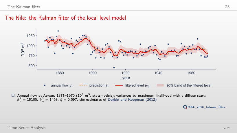
                  Slide 23: The Nile: the Kalman filter of the local level model
                  Slide 23
                    Question for the room ▶ takes q to 1. Where is the filtered level in 1899, the year with flow 774?
                    Answer

                    At 899, against 1037 at q̂ = 0.097: with q = 1, K̄ = 0.618, and the level takes almost two thirds of the surprise (757 in 1905). The level adapts to the dam faster, but it also follows isolated years.

                    Interpreting the Nile filter
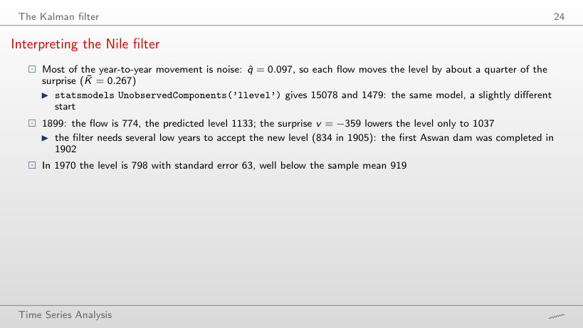
                    Slide 24: Interpreting the Nile filter
                    Slide 24
                      Question for the room Cut the sample at 1920. Does q̂ rise or fall compared to the full sample?
                      Answer

                      It rises, to 0.163 (0.097 on 1871–1970), with σ̂²ε = 19103. Over 50 years the 1899 break weighs more, and the likelihood attributes it to movement of the level.

                      Convergence of the Kalman gain and equivalence with SES
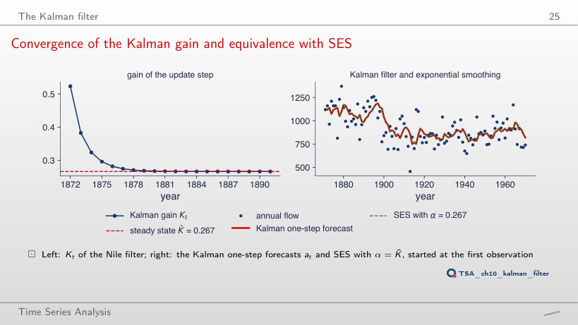
                      Slide 25: Convergence of the Kalman gain and equivalence with SES
                      Slide 25
                        Question for the room ▶ takes q to 1. From which year on is Kt within 0.001 of K̄?
                        Answer

                        From year 5 (from year 11 at q̂ = 0.097 and from year 17 at q = 0.03). With a large q, Pt settles quickly: every new observation dominates the uncertainty left by the diffuse start.

                        Smoothing, likelihood and missing data

                        Smoothing: using the whole sample
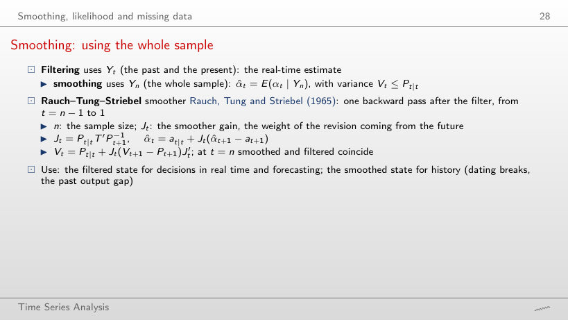
                        Slide 28: Smoothing: using the whole sample
                        Slide 28

                        Worked example

                        \[J_t=\frac{P_{t|t}}{P_{t+1}},\qquad \hat\alpha_t=a_{t|t}+J_t(\hat\alpha_{t+1}-a_{t+1}),\qquad V_t=P_{t|t}+J_t^2(V_{t+1}-P_{t+1})\]
                            Question for the room Move the year to 1898. What is the difference between the filtered and the smoothed level?
                            Answer

                            Filtered 1133, smoothed 1000: a difference of 134, larger than in 1897 (1145 against 1038, i.e. 107). The smoother uses the low years after 1899, so it lowers the level before the drop appears in the data.

                            The Nile: filtered against smoothed level
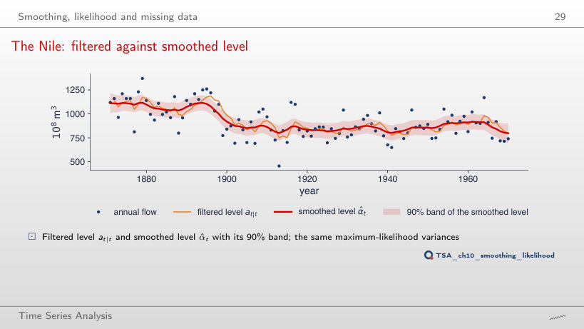
                            Slide 29: The Nile: filtered against smoothed level
                            Slide 29
                              Question for the room Set q = 0.001 (an almost constant level). What does the smoothed level look like around 1899?
                              Answer

                              Almost a straight line, falling slowly from 956 in 1897 to 881 in 1950: the step disappears. With a small q the model attributes the drop to noise, and the smoother cannot show a break that the model rules out.

                              The likelihood: prediction-error decomposition
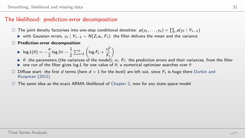
                              Slide 31: The likelihood: prediction-error decomposition
                              Slide 31

                              Worked example

                              \[\log L=\sum_{t=2}^{n}\ell_t,\qquad \ell_t=-\tfrac12\Big(\log 2\pi+\log F_t+\frac{v_t^2}{F_t}\Big)\]
                                  Question for the room At q̂ = 0.097, which year contributes the most negative term to log L?
                                  Answer

                                  1913 (ℓt = −9.78), a single very dry year; then 1916 (−9.18) and 1899 (−9.02). The year 1871 is not in the sum: the diffuse start gives it a huge Ft.

                                  Profile likelihood and the choice of q
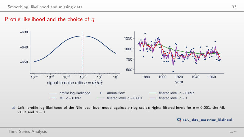
                                  Slide 33: Profile likelihood and the choice of q
                                  Slide 33
                                    Question for the room Take the chosen q to 10. What is the likelihood-ratio statistic against the maximum?
                                    Answer

                                    23.3, as far from the data as q = 0.001 (23.1); q = 1 gives 7.2. A level that chases every flood predicts one step ahead as badly as an almost constant level.

                                    Diagnostics of the Nile model
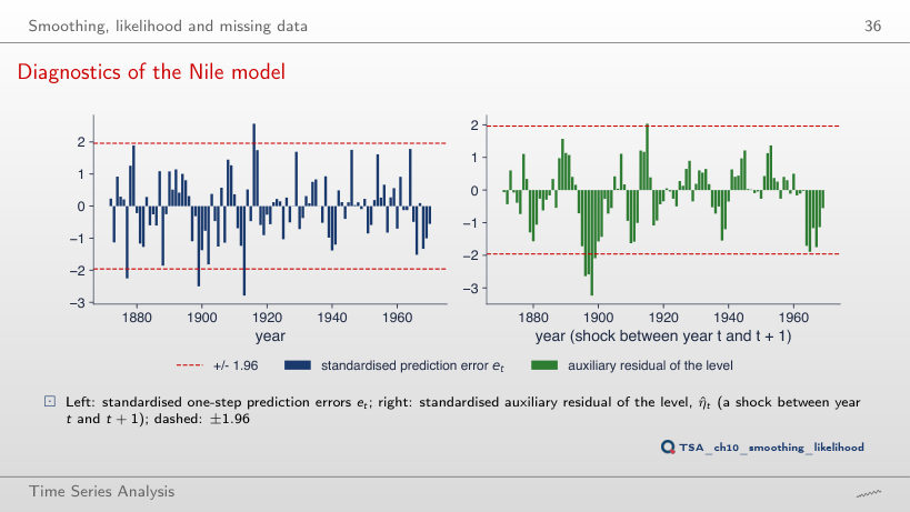
                                    Slide 36: Diagnostics of the Nile model
                                    Slide 36
                                      Question for the room Set q = 0.001. Is the Ljung–Box Q(10) test still passed?
                                      Answer

                                      No: Q(10) = 20.9, p = 0.022. An almost constant level leaves the drop after 1899 in the prediction errors, which become autocorrelated; at q̂ = 0.097, p = 0.21.

                                      Missing years and forecasts of the Nile
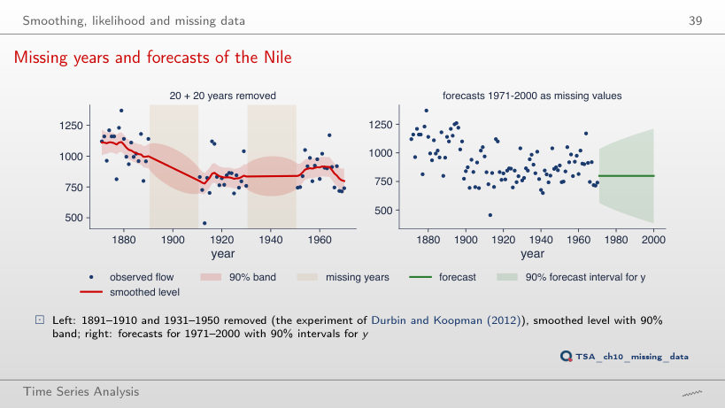
                                      Slide 39: Missing years and forecasts of the Nile
                                      Slide 39
                                        Question for the room Gaps of 10 years (1891–1900 and 1931–1940): what is the standard error of the smoothed level in 1895?
                                        Answer

                                        78, against 99 in 1900 with 20-year gaps and 48 with all data. The band grows with the distance to the nearest observed year.

                                        Trend, cycle and common factors

                                        The HP filter is a state space smoother
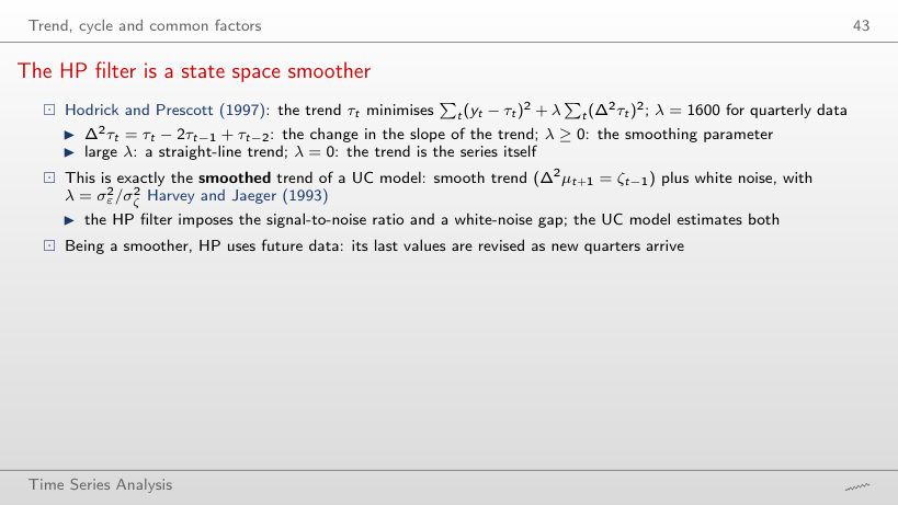
                                        Slide 43: The HP filter is a state space smoother
                                        Slide 43

                                        Worked example

                                        \[\min_{\tau}\sum_t(y_t-\tau_t)^2+\lambda\sum_t(\Delta^2\tau_t)^2\ \Longleftrightarrow\ y_t=\mu_t+\varepsilon_t,\ \ \Delta^2\mu_{t+1}=\zeta_{t-1},\ \ \lambda=\frac{\sigma^2_\varepsilon}{\sigma^2_\zeta}\]
                                            Question for the room ▶ takes λ to 100000. What becomes of the standard deviation of the HP gap?
                                            Answer

                                            5.5, against 2.9 at λ = 1600 and 1.3 at λ = 1: a stiffer trend leaves more of the movement of GDP in the gap.

                                            Romanian GDP: trend
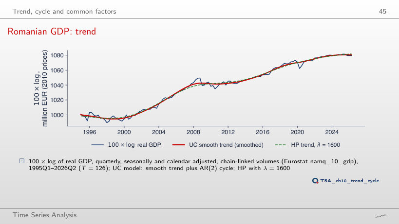
                                            Slide 45: Romanian GDP: trend
                                            Slide 45
                                              Question for the room Which λ of the grid brings the HP trend closest to the UC trend?
                                              Answer

                                              λ = 400: the largest distance is 0.63 points (1.01 at λ = 100 and 2.65 at λ = 1600). The UC trend is more flexible than the trend imposed by λ = 1600, so a smaller λ approximates it better.

                                              The Romanian output gap: three methods
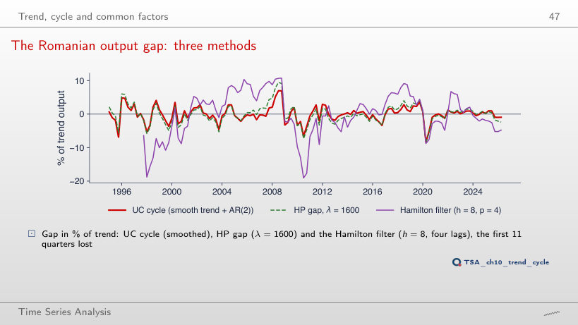
                                              Slide 47: The Romanian output gap: three methods
                                              Slide 47
                                                Question for the room ▶ takes h to 4. How does the standard deviation of the Hamilton gap change?
                                                Answer

                                                It falls to 4.6 (6.5 at h = 8 and 7.7 at h = 12): the residual of the regression contains the surprises of a shorter horizon.

                                                The output gap in real time and with the full sample
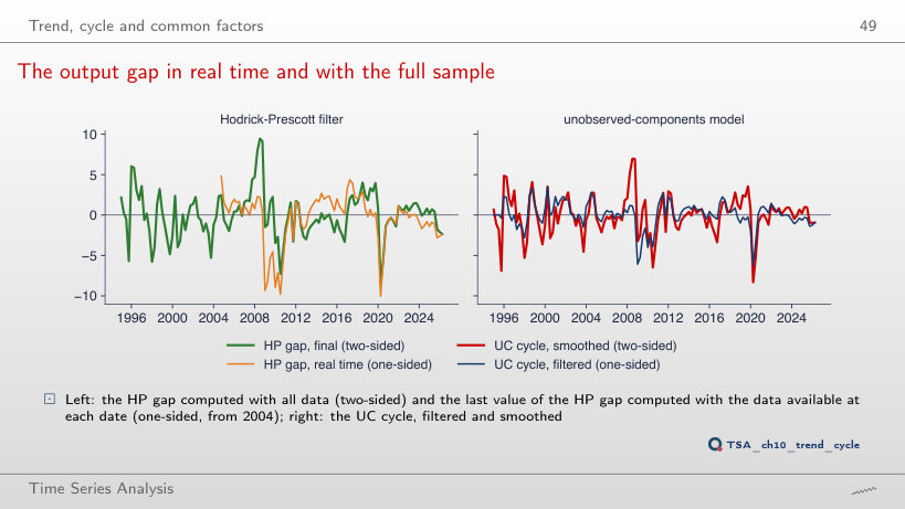
                                                Slide 49: The output gap in real time and with the full sample
                                                Slide 49
                                                  Question for the room Choose the data up to 2008Q3. What is the two-sided HP gap in 2008Q3?
                                                  Answer

                                                  2.2%, exactly the real-time value: at the end of the sample the two-sided filter becomes one-sided. With the data up to 2026Q2, the gap of 2008Q3 is 9.5%.

                                                  A time-varying beta: the BET and the euro area
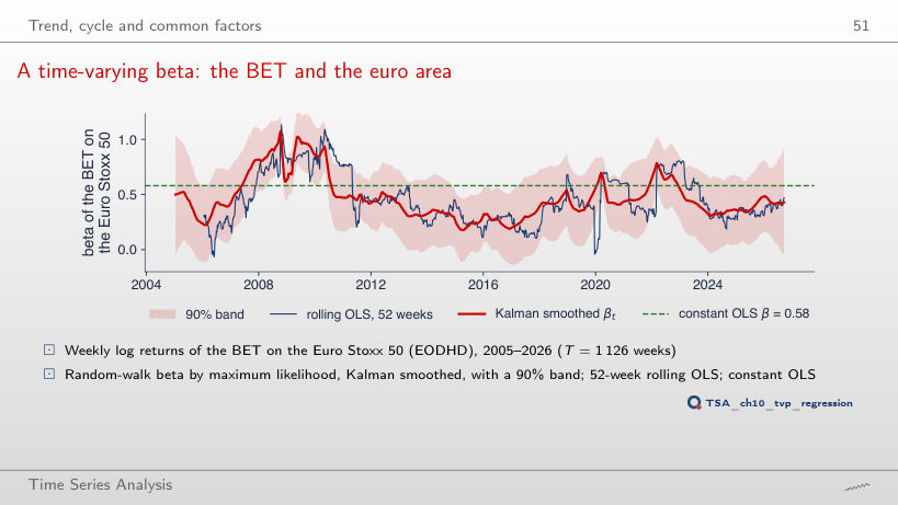
                                                  Slide 51: A time-varying beta: the BET and the euro area
                                                  Slide 51
                                                    Question for the room Set the variance of the beta shocks to 0. What becomes of the Kalman beta?
                                                    Answer

                                                    A flat line at 0.58, the OLS beta: with σ²β = 0 the Kalman filter computes the OLS estimate recursively, and the smoother gives every week the full-sample estimate.

                                                    A common factor of US activity
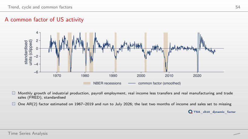
                                                    Slide 54: A common factor of US activity
                                                    Slide 54
                                                      Question for the room Without missing months (k = 0), what is the value of the factor for July 2026?
                                                      Answer

                                                      −0.78 with today’s FRED data, against −0.87 with two missing months (the slide, with the data of that time: −0.9). The factor uses whatever has arrived: missing income and sales move the latest value, they do not make it impossible to compute.

                                                      Markov switching

                                                      Transition matrix, durations and ergodic probabilities
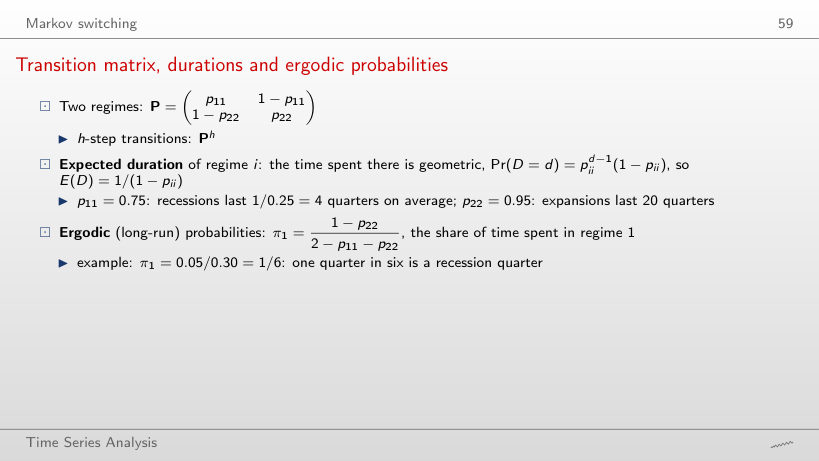
                                                      Slide 59: Transition matrix, durations and ergodic probabilities
                                                      Slide 59

                                                      Worked example

                                                      \[E(D_i)=\frac{1}{1-p_{ii}},\qquad \pi_1=\frac{1-p_{22}}{2-p_{11}-p_{22}},\qquad \Pr(S_{t+h}=1\mid S_t=1)=\pi_1+(1-\pi_1)(p_{11}+p_{22}-1)^h\]
                                                          Question for the room Set p11 = 0.5. How long does regime 1 last on average?
                                                          Answer

                                                          1/(1 − 0.5) = 2 periods. p11/(1 − p11) = 1 counts only the periods after the first, and 1/p11 is not a duration.

                                                          The Hamilton filter
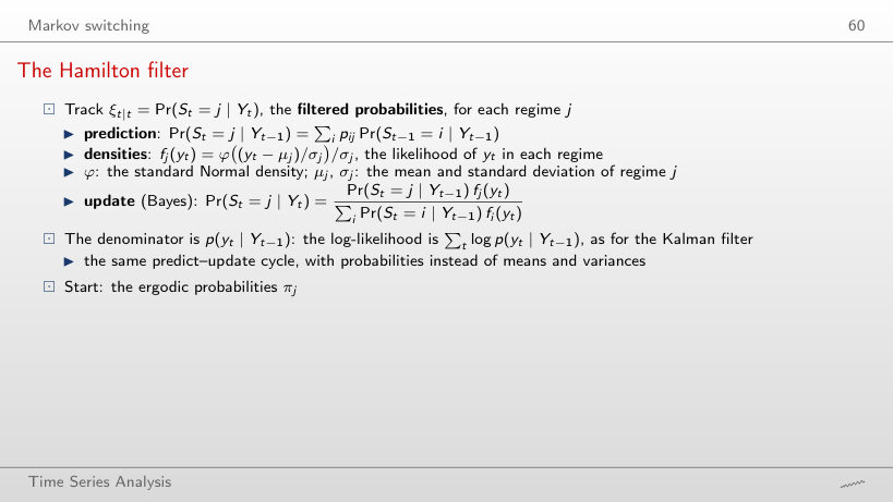
                                                          Slide 60: The Hamilton filter
                                                          Slide 60

                                                          Worked example

                                                          \[\Pr(S_t=j\mid Y_{t-1})=\sum_i p_{ij}\Pr(S_{t-1}=i\mid Y_{t-1}),\qquad \Pr(S_t=j\mid Y_t)=\frac{\Pr(S_t=j\mid Y_{t-1})\,f_j(y_t)}{\sum_i\Pr(S_t=i\mid Y_{t-1})\,f_i(y_t)}\]
                                                              Question for the room ▶ reaches 2008Q4 (growth −2.21%). What is the filtered probability of recession?
                                                              Answer

                                                              0.993: the prediction was 0.349, but f1(−2.21) is much larger than f2(−2.21), and Bayes’ rule takes the probability close to 1.

                                                              Hamilton's specification on today's data
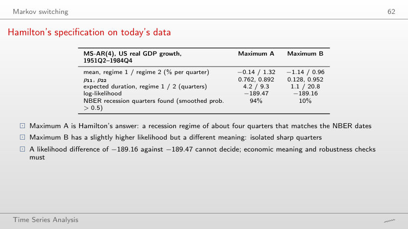
                                                              Slide 62: Hamilton's specification on today's data
                                                              Slide 62
                                                                Question for the room Raise the threshold to 0.7. Which share of the NBER recession quarters does maximum A still find?
                                                                Answer

                                                                90% (94% at the threshold 0.5); maximum B stays at 10%. The smoothed probabilities of maximum A are close to 0 or 1, so the threshold changes little.

                                                                US recessions from GDP growth
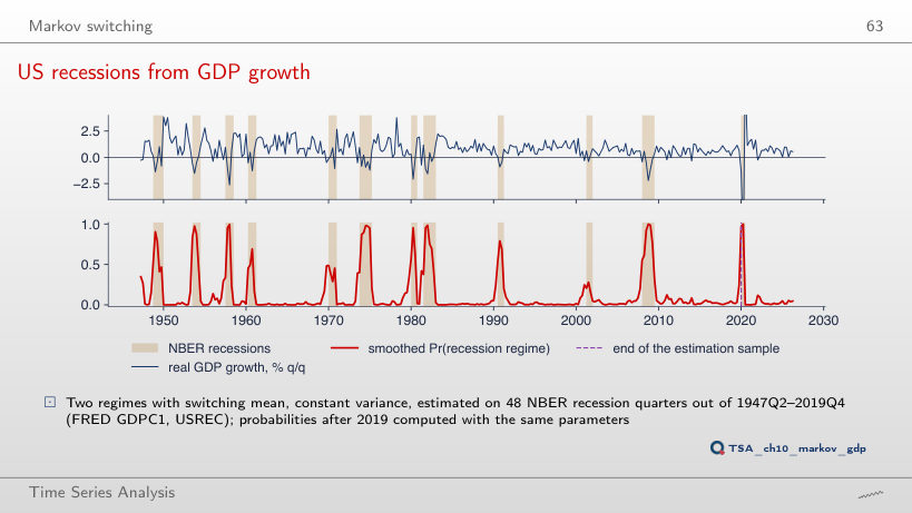
                                                                Slide 63: US recessions from GDP growth
                                                                Slide 63
                                                                  Question for the room Lower p11 to 0.3. What become the duration of a recession and the share of NBER quarters detected?
                                                                  Answer

                                                                  1.4 quarters and 39.6% (3.2 quarters and 62.5% at p̂11 = 0.685). A less persistent regime needs weaker data for every recession quarter, so short and mild recessions are no longer found; 2020Q2 keeps the probability 1.00.

                                                                  Filtered against smoothed probabilities: 2008
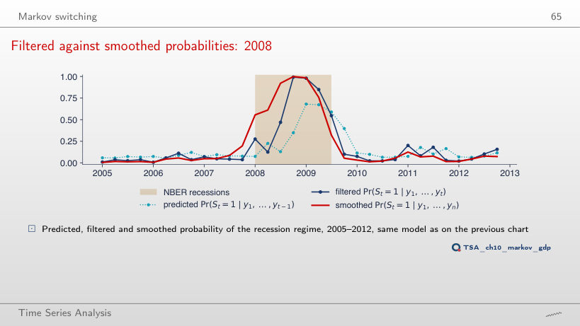
                                                                  Slide 65: Filtered against smoothed probabilities: 2008
                                                                  Slide 65
                                                                    Question for the room Choose the window 2000–2002 (the mild recession of 2001). Does the filtered probability cross 0.5?
                                                                    Answer

                                                                    No: its maximum is 0.38, and the smoothed one does not cross 0.5 either. The 2001 recession was too mild for the mean of −0.42% per quarter of the recession regime.

                                                                    Checks: which regimes did the model find?
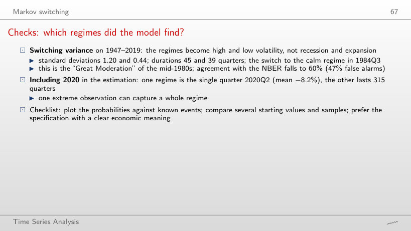
                                                                    Slide 67: Checks: which regimes did the model find?
                                                                    Slide 67
                                                                      Question for the room End the sample in 2020Q2. How many quarters form the low-mean regime?
                                                                      Answer

                                                                      One, 2020Q2 (mean −8.2%); on 1947–2019 the regime holds 30 quarters. A single extreme observation forms a regime on its own.

                                                                      Romanian GDP growth regimes
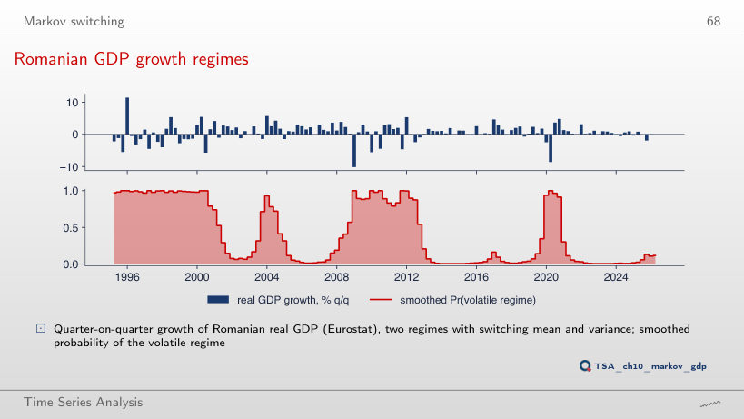
                                                                      Slide 68: Romanian GDP growth regimes
                                                                      Slide 68
                                                                        Question for the room Lower p11 of the volatile regime to 0.5. Which share of the quarters stays volatile?
                                                                        Answer

                                                                        29% (40% at p̂11 = 0.911): a less persistent volatile regime keeps only the quarters with large rises or falls.

                                                                        Calm and turbulent stock markets
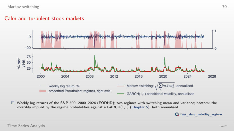
                                                                        Slide 70: Calm and turbulent stock markets
                                                                        Slide 70
                                                                          Question for the room Set p11 = 0.5 for the turbulent regime. Which share of the weeks stays turbulent?
                                                                          Answer

                                                                          12% (26% at p̂11 = 0.930). p11 = 0.5 does not mean a random classification: a turbulent regime that lasts two weeks on average remains only for the extreme weeks.

                                                                          Regime switching and spurious long memory
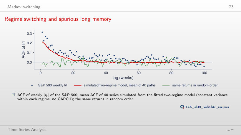
                                                                          Slide 73: Regime switching and spurious long memory
                                                                          Slide 73
                                                                            Question for the room ▶ adds simulated paths, from 1 to 40. Where does the mean ACF at lag 1 settle?
                                                                            Answer

                                                                            Around 0.21, below the 0.31 of the data: the regimes explain much of the short-run clustering, not all of it. The first path gives 0.26, the second 0.19: the mean over 40 paths removes the sampling variation.

                                                                            Recap: Markov switching
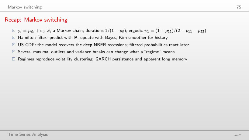
                                                                            Slide 75: Recap: Markov switching
                                                                            Slide 75
                                                                              Question for the room Which regime lasts longer in calendar time: the calm regime of the S&P 500 (36.8 periods) or the US expansion (19.7 periods)?
                                                                              Answer

                                                                              The US expansion: 19.7 quarters = 4.9 years, against 36.8 weeks = 0.7 years. The duration 1/(1 − pii) is in the time unit of the data.

                                                                              Annual flow of the Nile at Aswan, 1871–1970 (the statsmodels data set). Weekly S&P 500, BET and Euro Stoxx 50 prices (data/market, up to 18 September 2026). US real GDP growth and the NBER dates (FRED GDPC1, USREC), read with the chapter’s loader on 4 November 2026 and cut at 2026Q2, the last quarter of the slides; they reproduce the numbers of the lecture exactly. The four coincident indicators (FRED INDPRO, PAYEMS, W875RX1, CMRMTSPL), also read on 4 November 2026 and cut at July 2026: they have been revised since the slides were made; the parameters of the factor model (estimated on 1967–2019) are those of the lecture, but the latest months of the factor differ slightly (the July 2026 value: −0.87 with today’s data, −0.9 on the slide). Romanian real GDP (Eurostat namq_10_gdp) has been revised since the slides were made; the page uses the series of the slides, read from the vector line of the lecture chart (charts/tsa_ch10_ro_trend.pdf, all 126 quarters), which reproduces the numbers of the lecture to the sixth significant digit. The components of the UC model, the common factor, the probabilities of the two maxima of the MS-AR(4), the GARCH(1,1) volatility and the simulated regime paths come from the chapter’s code, with the same seed; the browser recomputes the Kalman filter and smoother, the likelihood, the diagnostics, the HP filter, the Hamilton (2018) filter, the real-time gaps, the time-varying beta, the Hamilton (1989) filter and the Kim smoother. Variants that do not appear in the lecture (another q, λ, h, sample end, p₁₁ or number of missing months) are extra runs of the chapter’s code with the same data; the chart “Checks: which regimes did the model find?” is an extra run for a slide that gives only numbers.