

Time Series Analysis

Chapter 2 · ARMA Models

The slide of the lecture is on the left, the same figure or table on the right, computed in the browser from the same data. The ▶ button moves the parameter step by step; the “Worked example” boxes redo the calculation with the numbers of the chapter.

Autoregressive models · Moving-average models · ARMA(p,q) models · Estimation · Model selection and diagnostics · Forecasting with ARMA models · Case study: Romanian GDP growth · More real series

Autoregressive models

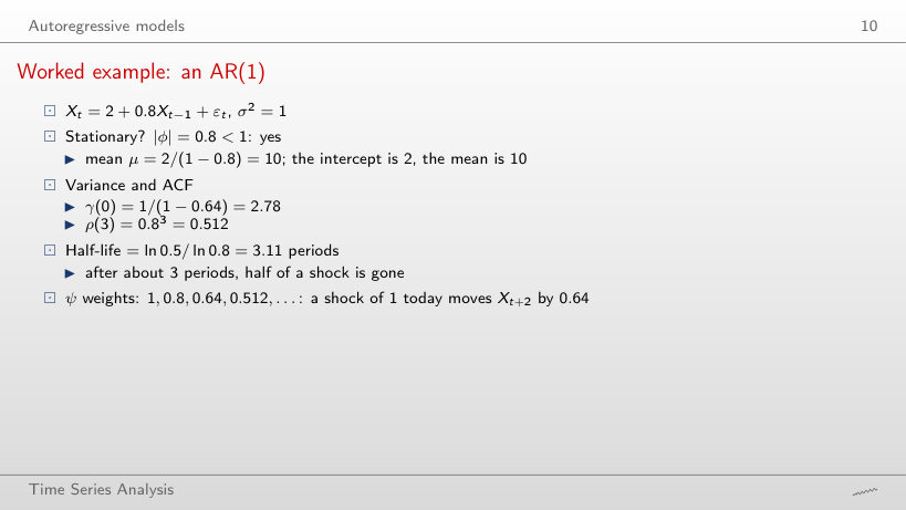
Worked example: an AR(1)
Slide 10: Worked example: an AR(1)
Slide 10

Worked example

\[\begin{gathered}X_t=c+\phi X_{t-1}+\varepsilon_t:\quad \mu=\frac{c}{1-\phi},\quad \gamma(0)=\frac{\sigma^2}{1-\phi^2},\\ \rho(h)=\phi^h,\quad h_{1/2}=\frac{\ln 0.5}{\ln|\phi|},\quad \psi_j=\phi^j\end{gathered}\]
      Question for the room In Xt = 2 + 0.8Xt−1 + εt, the intercept is 2. Is 2 the mean of the process?
      Answer

      No: μ = c/(1 − φ) = 2/0.2 = 10. The variance is γ(0) = 1/(1 − 0.64) = 2.78, ρ(3) = 0.512, and the half-life is 3.11 periods. With the same c and φ = 0.9, the mean rises to 20, γ(0) to 5.26 and the half-life to 6.58 periods.

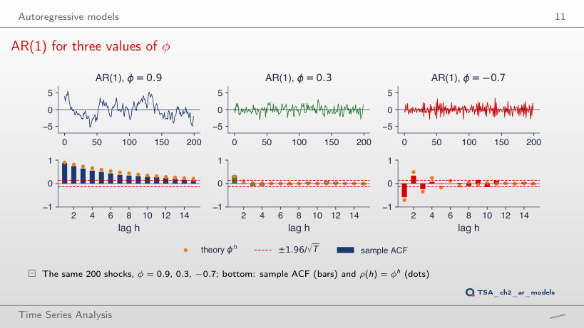
      AR(1) for three values of φ
      Slide 11: AR(1) for three values of φ
      Slide 11
        Question for the room With the same 200 shocks, the ▶ button raises φ in the left panel from 0 to 0.99; φ in the other two panels follows in proportion, up to 0.33 and −0.77. What happens in the left panel to ρ̂(1) and to the sample variance?
        Answer

        Both rise: ρ̂(1) goes from 0.10 to 0.95, and the sample variance from 1.04 to 14.5. The theoretical variance, 1/(1 − φ²), rises faster: 5.26 at φ = 0.9 and 50.3 at φ = 0.99. At φ = 0.9 the sample gives 4.98, below the theoretical value: a short path of a persistent process does not cover all its variation. With φ = −0.7 the sign of the autocorrelations alternates: ρ̂(1) = −0.58, ρ̂(2) = 0.34; at the end of the sweep, with φ = −0.77, ρ̂(1) = −0.66 and ρ̂(2) = 0.44.

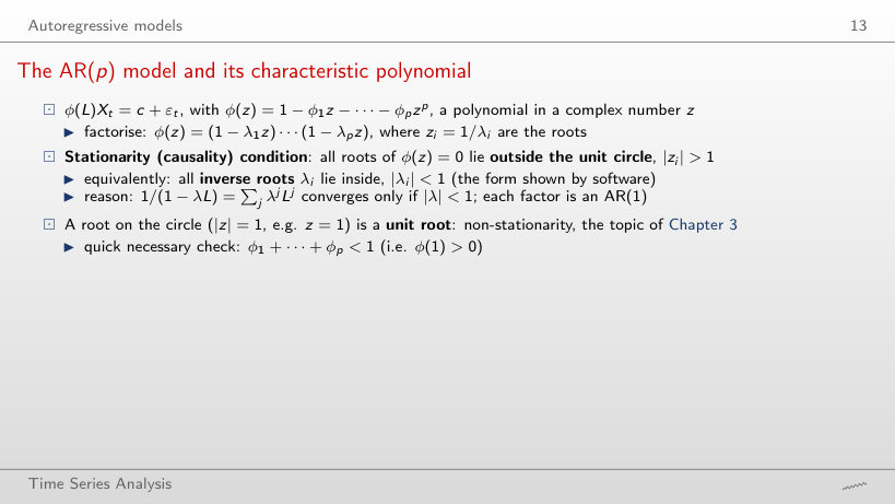
        The AR(p) model and its characteristic polynomial
        Slide 13: The AR(p) model and its characteristic polynomial
        Slide 13

        Worked example

        \[\begin{gathered}\phi(z)=1-\phi_1z-\phi_2z^2=0\ \Rightarrow\ z_{1,2}=\frac{-\phi_1\pm\sqrt{\phi_1^2+4\phi_2}}{2\phi_2},\\ \text{stationary}\iff |z_i|>1\iff \phi_1+\phi_2<1,\ \phi_2-\phi_1<1,\ |\phi_2|<1\end{gathered}\]
            Question for the room Example B has φ₁ = 1.0. Is the process stationary?
            Answer

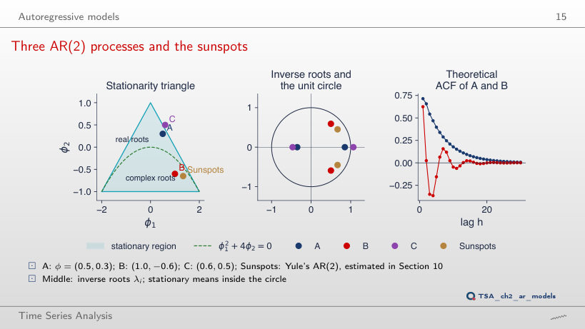
            Yes. The discriminant φ₁² + 4φ₂ = −1.4 is negative, the roots are complex, 0.833 ± 0.986i, with modulus 1.291 > 1 (the inverse roots have modulus 0.775). The triangle conditions hold: 0.4 < 1, −1.6 < 1, 0.6 < 1. Conversely, in example C both coefficients are below 1, yet the root 0.936 lies inside the unit circle.

            Three AR(2) processes and the sunspots
            Slide 15: Three AR(2) processes and the sunspots
            Slide 15
              Question for the room In example C, φ₁ = 0.6 and φ₂ = 0.5 are both below 1. Is the process stationary?
              Answer

              No. φ₁ + φ₂ = 1.1 > 1, so the point lies outside the triangle. The roots of 1 − 0.6z − 0.5z² are −2.14 and 0.936; the second lies inside the unit circle (its inverse root has modulus 1.068). Stationarity is read from the roots, not from the coefficients one at a time. B has complex roots, 0.833 ± 0.986i, with modulus 1.291: its ACF is a wave with a period of 7.2 lags, damped by 0.775 per lag.

              Moving-average models

              MA(1): θ = 0.8 and θ = -0.8
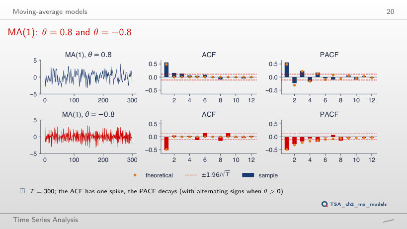
              Slide 20: MA(1): θ = 0.8 and θ = -0.8
              Slide 20
                Question for the room The ▶ button raises θ from 0 to 2. Can an MA(1) have ρ(1) above 0.5?
                Answer

                No. ρ(1) = θ/(1 + θ²) reaches its maximum of 0.5 at θ = 1 and then falls: at θ = 2 it is 0.4, the same as at θ = 0.5. At θ = ±0.8 the theoretical values are ±0.488, and the sample values, with T = 300, are 0.56 and −0.51. The ACF has a single non-zero value, while the PACF decays: φ̂₂₂ = −0.23 for θ = 0.8.

                The largest autocorrelation of an MA(1)
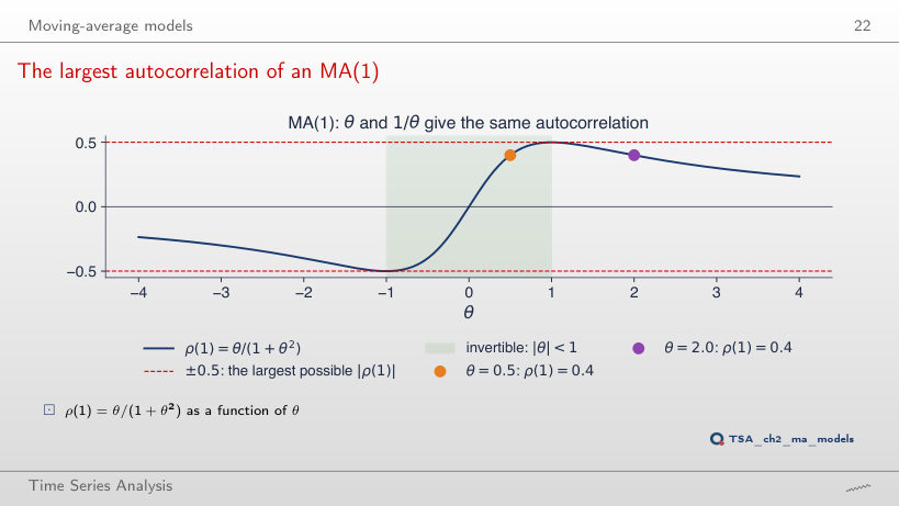
                Slide 22: The largest autocorrelation of an MA(1)
                Slide 22
                  Question for the room Which other value of θ gives the same ρ(1) = 0.4 as θ = 0.5, and which one do we keep?
                  Answer

                  θ = 2 = 1/0.5. The two models have the same ACF (with σ² multiplied by θ²), so the data cannot tell them apart: an identification problem. The invertibility convention, |θ| < 1, keeps θ = 0.5.

                  Worked example: θ = 2 or θ = 0.5?
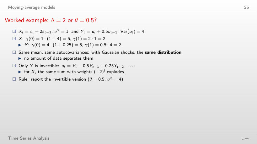
                  Slide 25: Worked example: θ = 2 or θ = 0.5?
                  Slide 25

                  Worked example

                  \[\begin{gathered}X_t=\varepsilon_t+\theta\varepsilon_{t-1}:\quad \gamma(0)=\sigma^2(1+\theta^2),\quad \gamma(1)=\theta\sigma^2;\\ (\theta,\sigma^2)\ \text{and}\ (1/\theta,\ \theta^2\sigma^2)\ \text{have the same ACF};\quad \varepsilon_t=\sum_{j\ge0}(-\theta)^jX_{t-j}\end{gathered}\]
                      Question for the room The ▶ button moves θ from −3 to 3. For which values is the MA(1) invertible, and what happens to the AR(∞) weights at θ = 2?
                      Answer

                      For |θ| < 1. At θ = 2 the weights (−θ)j are 1, −2, 4, −8, … and reach 256 at j = 8: the shocks cannot be recovered from the past of the series. The twin representation, θ = 0.5 with σ² = 4, has the weights 1, −0.5, 0.25, … and the same γ(0) = 5, γ(1) = 2.

                      ARMA(p,q) models

                      The ψ weights and the impulse response
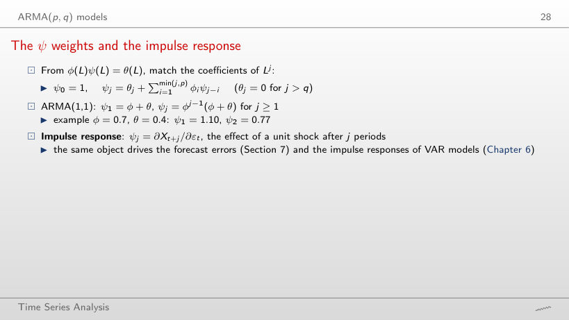
                      Slide 28: The ψ weights and the impulse response
                      Slide 28

                      Worked example

                      \[\begin{gathered}\psi_0=1,\quad \psi_j=\theta_j+\sum_{i=1}^{\min(j,p)}\phi_i\psi_{j-i};\\ \text{ARMA(1,1)}:\ \psi_j=\phi^{j-1}(\phi+\theta),\quad \sum_{j\ge0}\psi_j^2=1+\frac{(\phi+\theta)^2}{1-\phi^2}=\frac{\gamma(0)}{\sigma^2}\end{gathered}\]
                          Question for the room For φ = 0.7 and θ = 0.4, how many ψ weights cover at least 95% of γ(0)/σ² = 3.37?
                          Answer

                          Five, ψ₀…ψ₄: the cumulative sum of squares reaches 3.236, that is 95.9%; with ψ₀…ψ₃ it reaches 91.7%. ψ₁² = 1.21 alone accounts for 35.9%, more than the current shock (ψ₀² = 1, 29.7%), because ψ₁ = φ + θ = 1.10 > 1.

                          Impulse responses of four models
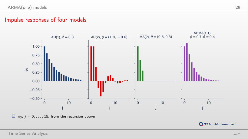
                          Slide 29: Impulse responses of four models
                          Slide 29
                            Question for the room In the ARMA(1,1) with φ = 0.7 and θ = 0.4, why is the first impulse response, ψ₁ = 1.10, above 1?
                            Answer

                            ψ₁ = φ + θ = 0.7 + 0.4 = 1.1: yesterday’s shock enters once through the MA term and once through the AR part. From j = 2 on, ψⱼ = φψⱼ₋₁: 0.77, 0.54, 0.38. The sum Σψⱼ² = 3.37 is the variance of the process in units of σ². For the MA(2) the response is exactly zero after two periods, and for the AR(2) with complex roots it changes sign: ψ₃ = −0.20, ψ₄ = −0.44. The ▶ button gives the first coefficient of the four models (θ₁ for the MA(2)) the same value, from 0 to 0.95 and back to 0.7: the AR responses last longer, the MA(2) response stays zero after j = 2.

                            Moments of the ARMA(1,1)
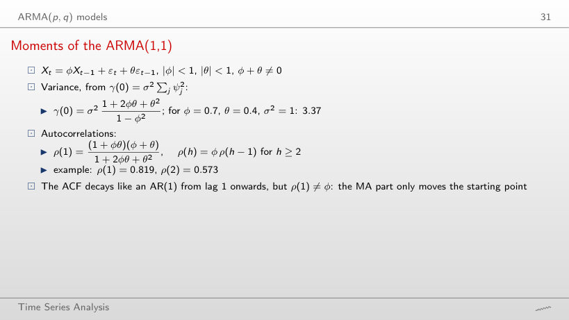
                            Slide 31: Moments of the ARMA(1,1)
                            Slide 31

                            Worked example

                            \[\gamma(0)=\sigma^2\frac{1+2\phi\theta+\theta^2}{1-\phi^2},\quad \rho(1)=\frac{(1+\phi\theta)(\phi+\theta)}{1+2\phi\theta+\theta^2},\quad \rho(h)=\phi\,\rho(h-1)\ \ (h\ge2)\]
                                Question for the room For φ = 0.7 and θ = 0.4, does the ACF start above or below φ? And for θ = −0.4?
                                Answer

                                Above: ρ(1) = 0.819 > 0.7. The difference ρ(1) − φ = θ(1 − φ²)/(1 + 2φθ + θ²) has the sign of θ, so with θ = −0.4 the ACF starts below φ: ρ(1) = 0.360, ρ(2) = 0.252, and γ(0) falls from 3.37 to 1.18. In both cases the ratio ρ(h)/φh is constant (1.169 and 0.514): after lag 1 the ACF decays like that of an AR(1).

                                Identification: the ACF–PACF table
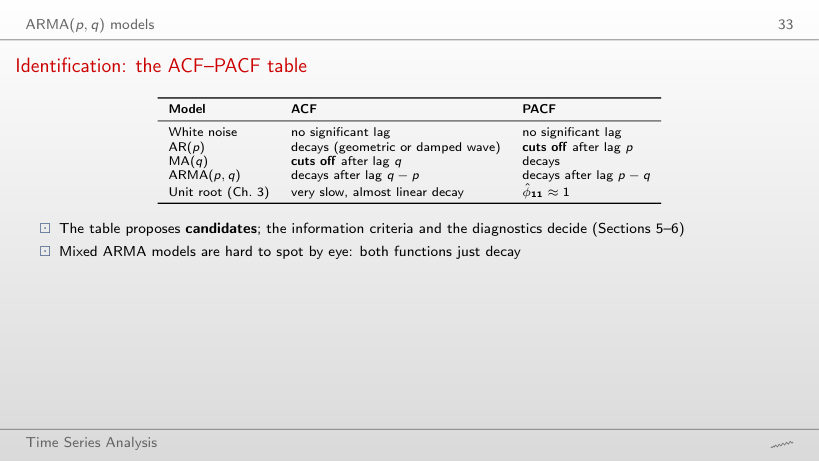
                                Slide 33: Identification: the ACF–PACF table
                                Slide 33
                                  Question for the room For the AR(2) with T = 500, the sample PACF leaves the band only at lags 1 and 2. Does the pattern survive with T = 100?
                                  Answer

                                  Yes for the PACF: the band widens to ±0.196 and the PACF still leaves it only at lags 1 and 2. The ACF leaves it at lags 1, 3, 4 and 5: the damped-wave decay is visible in the short sample too. For the MA(2) with T = 500, the ACF leaves the band at lags 1 and 2 and the PACF at lags 1–4: the table is read the other way round.

                                  Theoretical and sample ACF and PACF
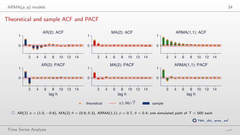
                                  Slide 34: Theoretical and sample ACF and PACF
                                  Slide 34
                                    Question for the room The ▶ button raises T from 50 to 500. What happens to the ±1.96/√T band and to the sample values?
                                    Answer

                                    The band narrows from ±0.28 to ±0.09, and the sample values move towards the theoretical ones. At T = 500, for the AR(2), φ̂₂₂ = −0.56 against φ₂₂ = −0.60; for the MA(2), ρ̂(1) = 0.51 and ρ̂(2) = 0.15 against 0.54 and 0.21. With short samples, the correlograms of different models can be confused.

                                    Estimation

                                    Worked example: Yule–Walker on Romanian GDP growth
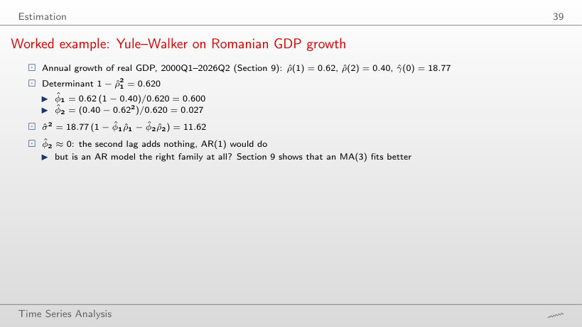
                                    Slide 39: Worked example: Yule–Walker on Romanian GDP growth
                                    Slide 39

                                    Worked example

                                    \[\hat R\hat\phi=\hat\rho:\quad \hat\phi_1=\frac{\hat\rho_1(1-\hat\rho_2)}{1-\hat\rho_1^2},\quad \hat\phi_2=\frac{\hat\rho_2-\hat\rho_1^2}{1-\hat\rho_1^2},\quad \hat\sigma^2=\hat\gamma(0)\big(1-\hat\phi_1\hat\rho_1-\hat\phi_2\hat\rho_2\big)\]
                                        Question for the room The slide writes 1 − ρ̂₁² = 0.620, but 1 − 0.62² = 0.616. Which value is right?
                                        Answer

                                        0.620, computed with the unrounded ρ̂₁ = 0.6167; 0.616 comes from rounding ρ̂₁ to 0.62. With the unrounded values, φ̂₁ = 0.600, φ̂₂ = 0.027 and σ̂² = 11.62, as on the slide (γ̂(0) = 18.77, dividing by T); with the rounded 0.62 and 0.40 one would get φ̂₁ = 0.604 and φ̂₂ = 0.025. On the sample that stops in 2019Q4, φ̂₂ = 0.102.

                                        Maximum likelihood
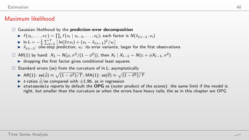
                                        Slide 40: Maximum likelihood
                                        Slide 40

                                        Worked example

                                        \[\begin{gathered}\ln L(\mu,\phi,\sigma^2)=-\tfrac12\ln\frac{2\pi\sigma^2}{1-\phi^2}-\frac{(1-\phi^2)(x_1-\mu)^2}{2\sigma^2}\\ -\sum_{t=2}^{T}\Big[\tfrac12\ln 2\pi\sigma^2+\frac{(x_t-\mu-\phi(x_{t-1}-\mu))^2}{2\sigma^2}\Big],\qquad \mathrm{se}(\hat\phi)=\Big(-\frac{d^2\ln L}{d\phi^2}\Big)^{-1/2}\end{gathered}\]
                                            Question for the room For the AR(1) on GDP growth, statsmodels reports se(φ̂) = 0.085, while the curvature of the log-likelihood gives 0.076. Which one matches the formula √((1 − φ̂²)/T)?
                                            Answer

                                            The curvature: 0.076, against 0.075 from the asymptotic formula. 0.085 is the OPG (outer product of gradients) standard error, the statsmodels default. The conclusion does not change: φ̂ = 0.630, the t-ratio is 8.3 with the curvature, and the 95% interval is [0.481; 0.779].

                                            Sampling distributions of the estimators
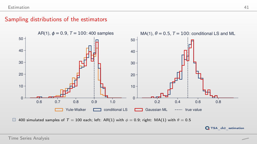
                                            Slide 41: Sampling distributions of the estimators
                                            Slide 41
                                              Question for the room With φ = 0.9 and T = 100, are the estimators of the AR(1) coefficient unbiased?
                                              Answer

                                              No. The means of the 400 estimates are 0.853 (Yule–Walker), 0.864 (conditional least squares) and 0.866 (MLE), all below 0.9; the approximation −(1 + 3φ)/T gives −0.037. The standard deviations, 0.054–0.056, exceed the asymptotic value 0.044. In the browser simulation with T = 400, the means rise to 0.889–0.891. For the MA(1) with θ = 0.5, the means are 0.504 and 0.506.

                                              Model selection and diagnostics

                                              Information criteria
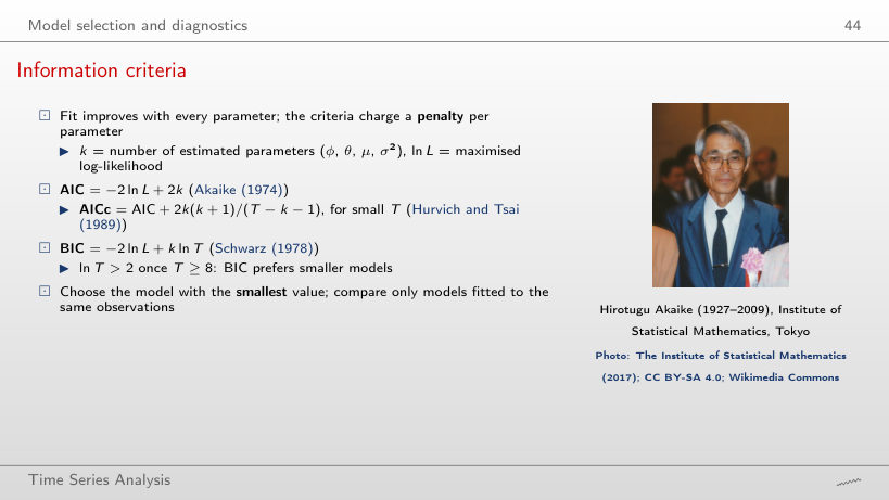
                                              Slide 44: Information criteria
                                              Slide 44

                                              Worked example

                                              \[k=p+q+2,\qquad \mathrm{AIC}=-2\ln L+2k,\qquad \mathrm{BIC}=-2\ln L+k\ln T,\qquad \mathrm{AICc}=\mathrm{AIC}+\frac{2k(k+1)}{T-k-1}\]
                                                  Question for the room ARMA(1,3) has a log-likelihood 1.54 higher than the MA(3). Why does BIC still prefer the MA(3)?
                                                  Answer

                                                  The extra parameter costs 2 in AIC and ln 106 = 4.66 in BIC, while −2 ln L falls by only 3.07. AIC therefore falls by 1.07 (548.97 against 550.04), and BIC rises by 1.59 (564.95 against 563.36). AICc, with the small-T correction, gives 549.82 and 550.64.

                                                  How often AIC and BIC find the true order
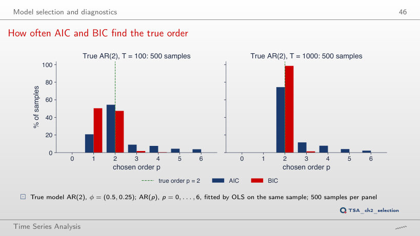
                                                  Slide 46: How often AIC and BIC find the true order
                                                  Slide 46
                                                    Question for the room With T = 1000, which criterion finds the true order p = 2 more often?
                                                    Answer

                                                    BIC, in 98.6% of the samples, against 74.4% for AIC, which picks an order that is too large in 25.6% of the cases. With T = 100 the ranking reverses: AIC 54.4%, BIC 47.4%, and BIC picks a model that is too small in 50.4% of the cases, because φ₂ = 0.25 is hard to detect in 100 observations.

                                                    Residual diagnostics
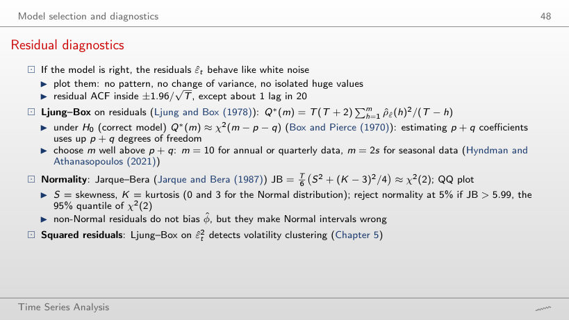
                                                    Slide 48: Residual diagnostics
                                                    Slide 48

                                                    Worked example

                                                    \[\begin{gathered}Q^*(m)=T(T+2)\sum_{h=1}^{m}\frac{\hat\rho_{\hat\varepsilon}(h)^2}{T-h}\approx\chi^2(m-p-q),\\ \mathrm{JB}=\frac{T}{6}\Big(S^2+\frac{(K-3)^2}{4}\Big)\approx\chi^2(2)\end{gathered}\]
                                                        Question for the room For the AR(1), Ljung–Box with m = 8 gives Q*(8) = 16.23. Do we reject at 5% that the residuals are uncorrelated?
                                                        Answer

                                                        Yes: with 8 − 1 = 7 degrees of freedom p = 0.023; even with the (wrong) 8 degrees of freedom p = 0.039. For the MA(3), Q*(8) = 5.35 with 5 degrees of freedom gives p = 0.375, so we do not reject. Normality is rejected for both: Jarque–Bera 25.9 for the AR(1) and 39.0 for the MA(3), above 5.99.

                                                        Why m - p - q degrees of freedom
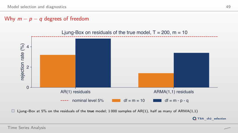
                                                        Slide 49: Why m - p - q degrees of freedom
                                                        Slide 49
                                                          Question for the room The residuals of the true ARMA(1,1) are tested with Ljung–Box, m = 10, at 5%. How often does the test reject with 10 degrees of freedom?
                                                          Answer

                                                          In 1.4% of the samples, not in 5%: the estimated residuals are less correlated than true white noise at the first lags. With m − p − q = 8 degrees of freedom the rate is 3.4%; for the AR(1), 3.2% with 10 and 4.8% with 9. At m = 3 the gap widens: for the ARMA(1,1), 0.2% with 3 degrees of freedom and 4.8% with 1.

                                                          Forecasting with ARMA models

                                                          Worked example: forecasting an AR(1)
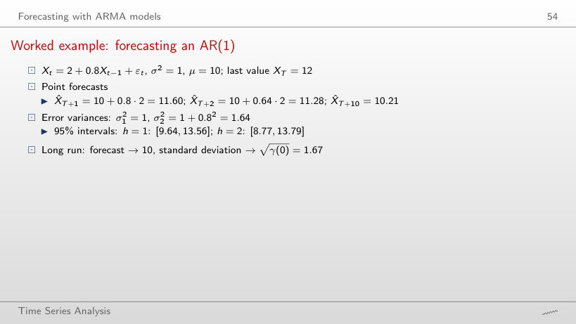
                                                          Slide 54: Worked example: forecasting an AR(1)
                                                          Slide 54

                                                          Worked example

                                                          \[\begin{gathered}\hat X_{T+h|T}=\mu+\phi^h(X_T-\mu),\quad \hat X_{T+h|T}\pm1.96\,\sigma_h,\\ \sigma_h^2=\sigma^2\sum_{j=0}^{h-1}\psi_j^2=\sigma^2\frac{1-\phi^{2h}}{1-\phi^2}\end{gathered}\]
                                                              Question for the room For Xt = 2 + 0.8Xt−1 + εt, towards which width does the 95% forecast interval tend?
                                                              Answer

                                                              Towards 2 × 1.96 × √γ(0) = 2 × 1.96 × 1.67 = 6.53. The width is 3.92 at h = 1, 5.02 at h = 2 and 6.50 at h = 10: uncertainty grows fast over the first horizons, then settles at the unconditional level.

                                                              Mean reversion in forecasts
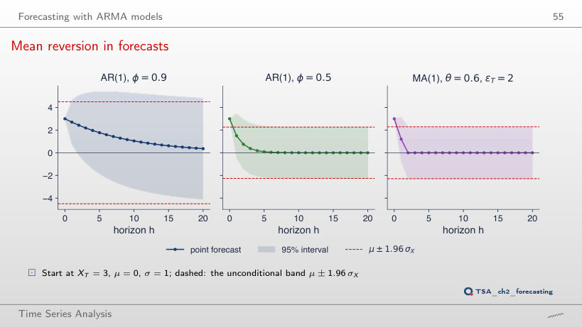
                                                              Slide 55: Mean reversion in forecasts
                                                              Slide 55
                                                                Question for the room Starting from XT = 3, what is the forecast 5 periods ahead for the AR(1) with φ = 0.9 and with φ = 0.5?
                                                                Answer

                                                                1.77 for φ = 0.9 (standard error 1.85) and 0.094 for φ = 0.5, practically the mean. The interval approaches the unconditional band μ ± 1.96σX, with σX = 2.29 for φ = 0.9 and 1.15 for φ = 0.5. For the MA(1) only the first step is informative, θεT = 1.2; from h = 2 on, the forecast is the mean and the interval has its long-run width. The ▶ button moves XT from 3 to −4 and back: the AR(1) forecasts return to the mean from any starting point, and the intervals do not change, because the standard errors do not depend on XT.

                                                                Case study: Romanian GDP growth

                                                                Step 1: identification
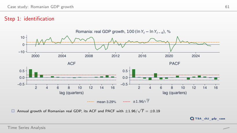
                                                                Slide 61: Step 1: identification
                                                                Slide 61
                                                                  Question for the room The ACF of annual GDP growth cuts off after lag 3. Does the pattern remain if the sample stops in 2019Q4, before the pandemic?
                                                                  Answer

                                                                  Yes. With 80 quarters, the first autocorrelations are 0.62, 0.45 and 0.24, then 0.04 at lag 4, inside the ±0.22 band. On the full sample of 106 quarters: 0.62, 0.40, 0.21 and −0.01. The pattern comes from the construction of the series: the annual rate is the sum of four quarterly rates, and consecutive annual rates share three quarters. Ljung–Box Q*(8) = 64.9 on the full sample.

                                                                  Step 2: estimation and information criteria
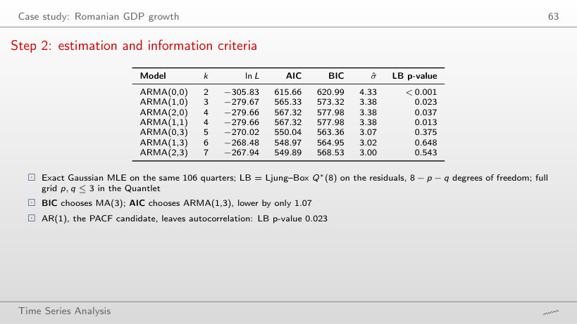
                                                                  Slide 63: Step 2: estimation and information criteria
                                                                  Slide 63
                                                                    Question for the room Over the whole grid p, q ≤ 3, which model has the smallest AICc, and by how much does it beat the MA(3)?
                                                                    Answer

                                                                    ARMA(1,3), with AICc 549.82 against 550.64 for the MA(3), a difference of 0.82. On AIC, ARMA(2,3) is second, 0.92 above the minimum, ahead of the MA(3) (1.07), and ARMA(3,3) is 2.37 above. On BIC, the MA(3) has 563.36 and ARMA(1,3) follows 1.59 higher.

                                                                    Interpreting the estimated MA(3)
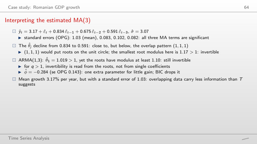
                                                                    Slide 64: Interpreting the estimated MA(3)
                                                                    Slide 64

                                                                    Worked example

                                                                    \[\begin{gathered}\hat y_t=\hat\mu+\hat\varepsilon_t+\hat\theta_1\hat\varepsilon_{t-1}+\hat\theta_2\hat\varepsilon_{t-2}+\hat\theta_3\hat\varepsilon_{t-3},\\ \text{invertible}\iff \theta(z)=1+\theta_1z+\theta_2z^2+\theta_3z^3\ne0\ \ \text{for}\ |z|\le1\end{gathered}\]
                                                                        Question for the room In the ARMA(1,3), θ̂₁ = 1.019 > 1. Is the model invertible?
                                                                        Answer

                                                                        Yes: the roots of θ(z) have moduli 1.102, 1.181 and 1.181, all above 1. For q > 1 invertibility is read from the roots, not from the coefficients one at a time. The AR coefficient, φ̂ = −0.284 with se 0.143, has a t-ratio of −1.98, just beyond the 1.96 threshold.

                                                                        Step 3: diagnostics of the MA(3)
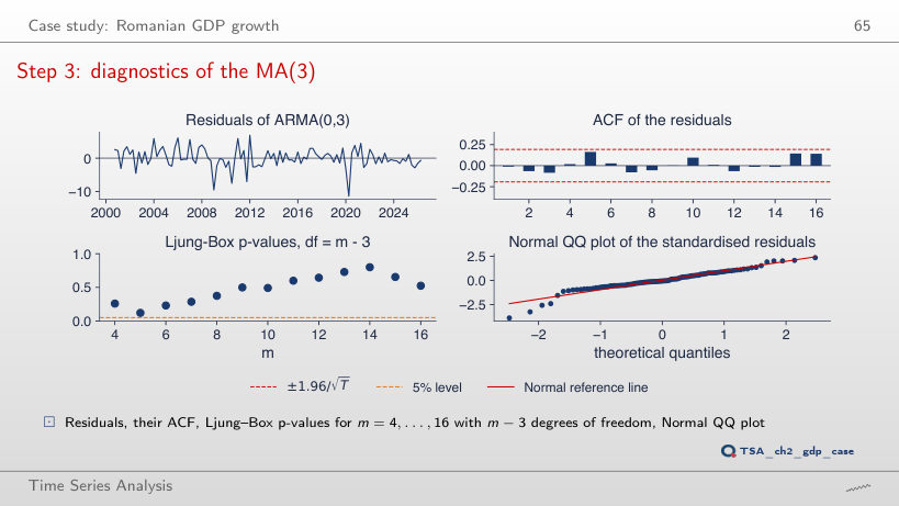
                                                                        Slide 65: Step 3: diagnostics of the MA(3)
                                                                        Slide 65
                                                                          Question for the room For the MA(3), the Ljung–Box test with m = 8 gives p = 0.375 with 5 degrees of freedom. Which p-value would it give with 8 degrees of freedom?
                                                                          Answer

                                                                          0.720, a conclusion that is too reassuring: the degrees of freedom must be reduced by the number of estimated ARMA parameters. The residuals are not Normal: Jarque–Bera 39.0, p < 0.001, skewness −0.75, kurtosis 5.61; the largest residual, −11.4 in 2020Q2, is −3.89 standard deviations. The AR(1) leaves correlation in the residuals: Q*(8) = 16.2 with 7 degrees of freedom, p = 0.023.

                                                                          Step 4: forecasts
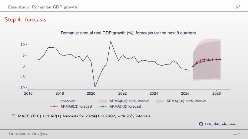
                                                                          Slide 67: Step 4: forecasts
                                                                          Slide 67
                                                                            Question for the room From which horizon on is the MA(3) forecast constant?
                                                                            Answer

                                                                            From the fourth quarter: −0.14, 1.81, 2.77, then the mean of 3.17%. After q = 3 steps the model only knows the mean. The AR(1) returns gradually: 2.99% after 8 quarters, with a mean of 3.12%. The 95% intervals are [−6.1, 5.9] for one quarter and [−6.3, 12.7] from four quarters on. With the origin in 2019Q4, both models forecast more than 3.8% for 2020, while the series falls to −9.9% in 2020Q2.

                                                                            Interpreting the GDP forecasts
                                                                            Slide 68: Interpreting the GDP forecasts
                                                                            Slide 68

                                                                            Worked example

                                                                            \[\begin{gathered}\sigma_h^2=\hat\sigma^2\sum_{j=0}^{h-1}\hat\psi_j^2;\\ \text{MA(3)}:\ \hat\psi_j=\hat\theta_j,\ \ \sigma_h^2=\hat\sigma^2(1+\hat\theta_1^2+\hat\theta_2^2+\hat\theta_3^2)\ \ (h\ge4)\end{gathered}\]
                                                                                Question for the room Why does the MA(3) interval stop widening after h = 4, while the AR(1) interval keeps growing?
                                                                                Answer

                                                                                For the MA(3), ψj = 0 for j > 3, so σh stays at σ̂√(1 + θ̂₁² + θ̂₂² + θ̂₃²) = 3.07 × √2.50 = 4.85 from h = 4 on. For the AR(1), σh grows from 3.38 to 4.35 at h = 8. The width of the 95% interval goes from 12.0 to 19.0 for the MA(3) and from 13.2 to 17.0 for the AR(1). With the origin in 2019Q4, the RMSE over the 8 observed quarters is 7.41 for the MA(3) and 7.06 for the AR(1).

                                                                                More real series

                                                                                Romanian inflation: an AR(2) forecast
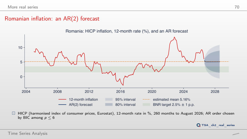
                                                                                Slide 70: Romanian inflation: an AR(2) forecast
                                                                                Slide 70
                                                                                  Question for the room Towards which value does the AR(2) forecast return: the BNR target or the estimated mean?
                                                                                  Answer

                                                                                  Towards the estimated mean, 5.16%, the average of 2005–2026, not towards the 2.5% target: from 6.09% in August 2026 to 5.44% in September and 5.13% in August 2028. φ̂₁ + φ̂₂ = 0.976 and the largest inverse root has modulus 0.963, so the return is slow. The Ljung–Box test on the residuals rejects: Q*(12) = 71.6 with 10 degrees of freedom, p < 0.001.

                                                                                  Daily returns: BET and EUR/RON
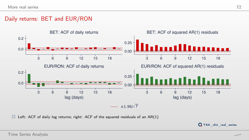
                                                                                  Slide 72: Daily returns: BET and EUR/RON
                                                                                  Slide 72
                                                                                    Question for the room For the BET, φ̂ = 0.109 is highly significant. Does the AR(1) explain a large part of the variation of daily returns?
                                                                                    Answer

                                                                                    No: R² is 1.2% for the BET and 2.9% for EUR/RON. The effect is real statistically but small economically. The squared residuals are strongly autocorrelated (Ljung–Box Q*(10) = 2496 for the BET and 2351 for EUR/RON), and the kurtosis of the residuals is 14.0 and 17.0: the model describes the mean, not the variance.

                                                                                    Interpreting the AR(1) for daily returns
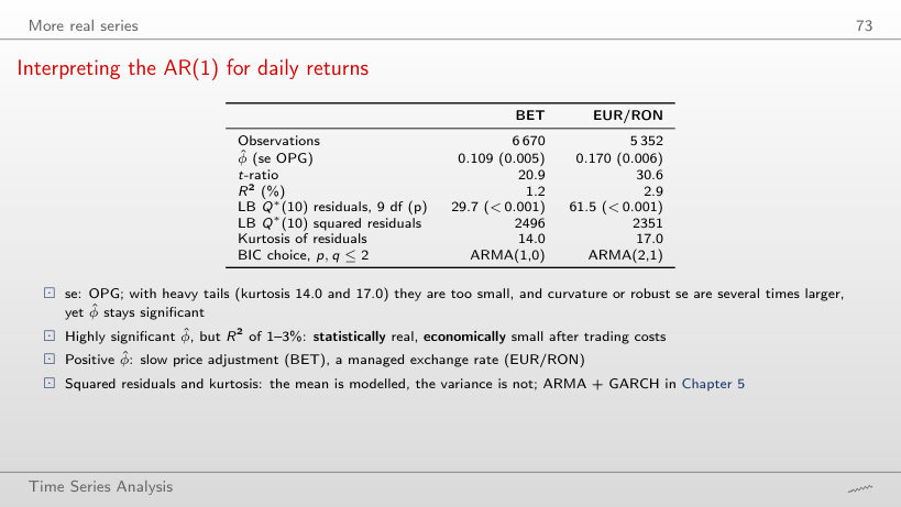
                                                                                    Slide 73: Interpreting the AR(1) for daily returns
                                                                                    Slide 73

                                                                                    Worked example

                                                                                    \[\mathrm{se}_{\text{OPG}}=\Big[\Big(\sum_t s_ts_t^\top\Big)^{-1}\Big]_{\phi\phi}^{1/2},\qquad \mathrm{se}_{\text{classical}}\approx\sqrt{\frac{1-\hat\phi^2}{T}},\qquad t=\frac{\hat\phi}{\mathrm{se}}\]
                                                                                        Question for the room The slide gives the BET a t-ratio of 20.9. Is this the t-ratio from the classical standard error?
                                                                                        Answer

                                                                                        No. The standard error of the slide, 0.0052, is the OPG one, the statsmodels default; the classical standard error, from the curvature of the log-likelihood, is 0.0122, close to √((1 − φ̂²)/T) = 0.0122, and the t-ratio is 9.0. For EUR/RON, 12.6 instead of 30.6. The coefficients remain highly significant, but R² is 1.2% and 2.9%.

                                                                                        The sunspots: AR(2) and the information criteria
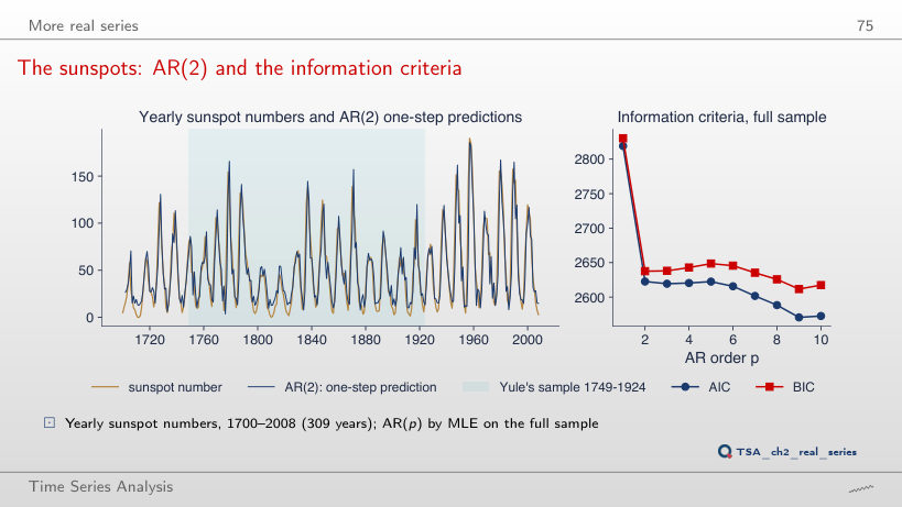
                                                                                        Slide 75: The sunspots: AR(2) and the information criteria
                                                                                        Slide 75
                                                                                          Question for the room What period of the solar cycle does Yule's AR(2), estimated on 1749–1924, imply?
                                                                                          Answer

                                                                                          10.6 years. The estimated coefficients, φ̂₁ = 1.336 and φ̂₂ = −0.650, give complex roots; the period is 2π/arccos(φ̂₁/(2√−φ̂₂)) = 10.6, and the modulus of the inverse root is 0.806. On the full sample, the AR(2) explains 83% of the variance one year ahead, and AIC and BIC both pick p = 9 among p ≤ 10.

                                                                                          Simulations: shocks from the Normal distribution, drawn with the seeds of the chapter code; when the parameters differ from those of the lecture, the simulation is redone in the browser. GDP: Eurostat, chain-linked volumes (2010), not seasonally adjusted, in the version used in the lecture. HICP: Eurostat, up to August 2026. BET: EODHD; EUR/RON: BNR reference rate. Sunspots: the statsmodels data set, 1700–2008.