

Time Series Analysis

Chapter 8 · Long Memory and ARFIMA

The slide of the lecture is on the left, the same figure or table on the right, computed in the browser from the same data. The ▶ button moves the parameter step by step; the “Worked example” boxes redo the calculation with the numbers of the chapter.

Short and long memory · Fractional differencing · The ARFIMA(p,d,q) model · Estimating d · Forecasting with ARFIMA · Long memory in volatility · Spurious long memory

Short and long memory

Four persistent series
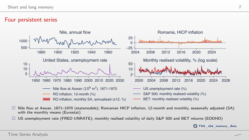
Slide 7: Four persistent series
Slide 7
    Question for the room For how many consecutive months, at most, does US unemployment stay on one side of its 1948–2026 mean?
    Answer

    106 months, almost nine years; the Nile stays 11 years on one side of its mean, Romanian 12-month inflation 103 months. For a series without memory such long runs would be very rare.

    Sample ACF against an AR(1)
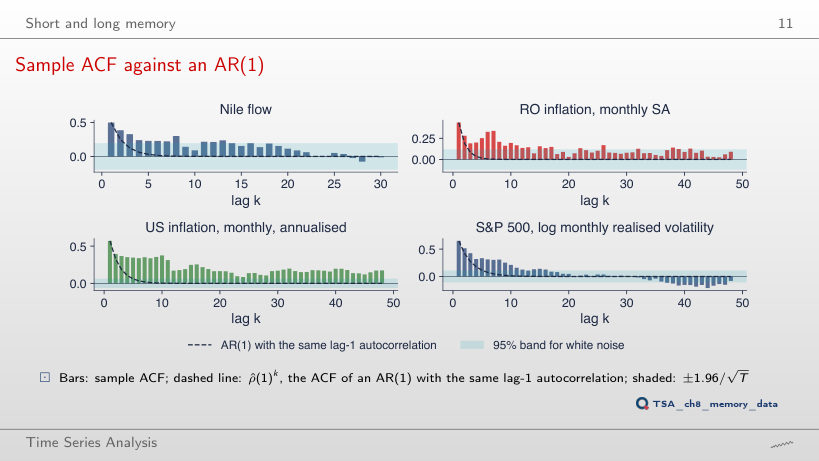
    Slide 11: Sample ACF against an AR(1)
    Slide 11
      Question for the room Drop the first 50% of each sample (US inflation then starts in November 1986). How many of the 48 autocorrelations of US monthly inflation stay above the band?
      Answer

      11 of 48, against 48 of 48 on 1947–2026; ρ̂(10) falls from 0.38 to 0.16. Much of the memory of the full series comes from the 1970s and early 1980s.

      Hyperbolic against exponential decay
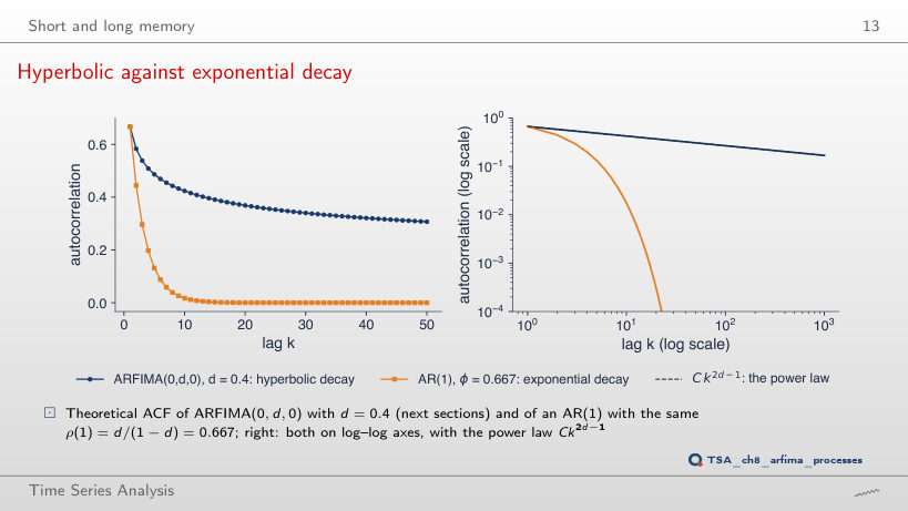
      Slide 13: Hyperbolic against exponential decay
      Slide 13
        Question for the room Set d = 0.2. What is ρ(10) for ARFIMA(0, 0.2, 0) and for the AR(1) with the same ρ(1) = 0.25?
        Answer

        0.064 against 9.5 · 10⁻⁷. With a small d the hyperbolic tail is low, but still five orders of magnitude above the exponential one.

        Interpreting the two decay laws
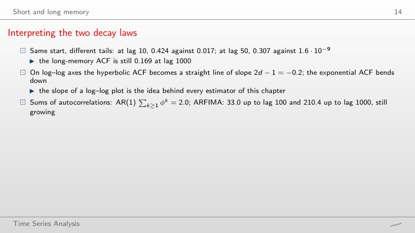
        Slide 14: Interpreting the two decay laws
        Slide 14

        Worked example

        \[\rho(k)=\frac{\Gamma(k+d)\,\Gamma(1-d)}{\Gamma(k-d+1)\,\Gamma(d)}\approx C\,k^{2d-1},\quad C=\frac{\Gamma(1-d)}{\Gamma(d)};\qquad \rho_{AR}(k)=\phi^k,\ \ \phi=\frac{d}{1-d}\]
            Question for the room Set d = 0.1. How many times larger is the sum of the first 1000 ARFIMA autocorrelations than the full sum of the AR(1)?
            Answer

            14 times: 1.74 against 0.125. Even a weak long memory accumulates far more than a short memory with the same ρ(1).

            Fractional differencing

            Worked example: the weights of (1-L)^0.4
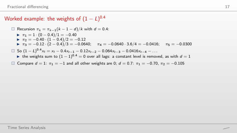
            Slide 17: Worked example: the weights of (1-L)^0.4
            Slide 17

            Worked example

            \[\pi_0=1,\qquad \pi_k=\pi_{k-1}\,\frac{k-1-d}{k},\qquad (1-L)^d x_t=\sum_{k\ge0}\pi_k x_{t-k},\qquad \sum_{k\ge0}\pi_k=(1-1)^d=0\]
                Question for the room Set d = 1.5. What are π₁ and π₂, and what sign has π₂?
                Answer

                π₁ = −1.5 and π₂ = −1.5 · (1 − 1.5)/2 = +0.375. For d > 1 the factor (k − 1 − d) is negative at k = 2, so the weights change sign after the first lag.

                Fractional differencing and fractional integration
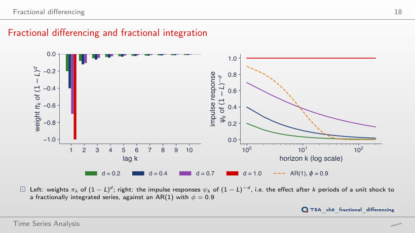
                Slide 18: Fractional differencing and fractional integration
                Slide 18
                  Question for the room Move the blue curve to d = 0.9. What share of a unit shock is left after 100 periods?
                  Answer

                  ψ₁₀₀ = 0.59 (0.74 after 10 periods), against 0.9¹⁰⁰ = 2.7 · 10⁻⁵ for the AR(1) with φ = 0.9. The series reverts to its mean, but very slowly.

                  The degree of differencing a price needs
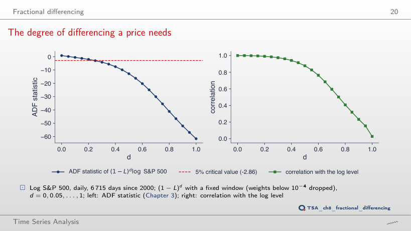
                  Slide 20: The degree of differencing a price needs
                  Slide 20
                    Question for the room Choose the threshold 10⁻³ (a shorter window). From which d does the ADF statistic pass the 5% critical value, and with how many weights?
                    Answer

                    From d = 0.35, with 61 weights, against 0.25 with 445. The truncated weights no longer sum to 0, so the filter keeps part of the level and a larger d is needed for stationarity.

                    The ARFIMA(p,d,q) model

                    The parameter d: what each range means
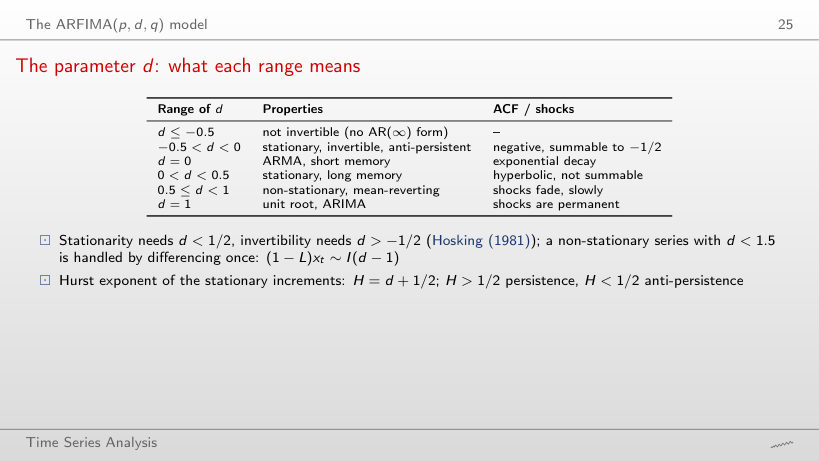
                    Slide 25: The parameter d: what each range means
                    Slide 25
                      Question for the room Set d = 0.6. Is the series stationary, and what is its first difference?
                      Answer

                      It is not stationary (d ≥ 0.5) but it reverts to its mean: ψ₁₀₀ = 0.11. The first difference is ARFIMA(0, −0.4, 0), anti-persistent with ρ(1) = −0.29.

                      Worked example: ARFIMA(0, 0.3, 0)
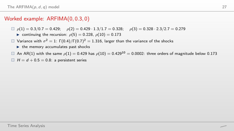
                      Slide 27: Worked example: ARFIMA(0, 0.3, 0)
                      Slide 27

                      Worked example

                      \[\rho(1)=\frac{d}{1-d},\quad \rho(k)=\rho(k-1)\,\frac{k-1+d}{k-d},\quad \gamma(0)=\sigma^2\,\frac{\Gamma(1-2d)}{\Gamma(1-d)^2},\quad H=d+\tfrac12\]
                          Question for the room Set d = 0.45. What are ρ(1) and ρ(10)?
                          Answer

                          ρ(1) = 0.818 and ρ(10) = 0.652; an AR(1) with the same ρ(1) has ρ(10) = 0.134. The variance rises to 3.64.

                          ARFIMA(0,d,0) with d = 0.4 and d = -0.4
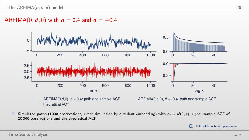
                          Slide 28: ARFIMA(0,d,0) with d = 0.4 and d = -0.4
                          Slide 28
                            Question for the room Set d = 0.45. What is the theoretical variance of the series (σ² = 1)?
                            Answer

                            Γ(0.1)/Γ(0.55)² = 3.64. The variance of the 1000-observation path is only 2.31: the sample mean absorbs part of the slow component.

                            Fractional Brownian motion for three Hurst exponents
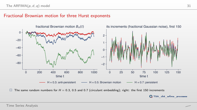
                            Slide 31: Fractional Brownian motion for three Hurst exponents
                            Slide 31
                              Question for the room Move H to 0.05 and 0.95 (Δ = 0.45). What is the lag-1 autocorrelation of the increments for H = 0.95, in theory and in the sample?
                              Answer

                              In theory 20.9 − 1 = 0.87, in the sample 0.72. With such strong persistence the mean of the 1000 increments absorbs part of the dependence, so the sample ACF is biased downwards.

                              Estimating d

                              The R/S statistic, step by step
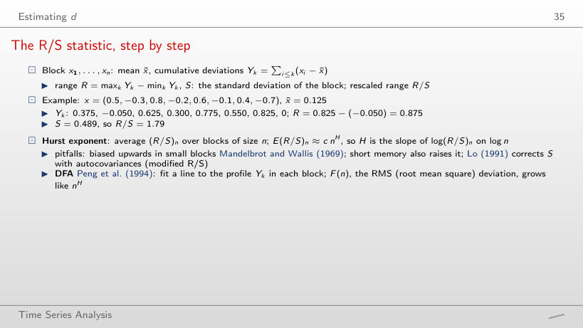
                              Slide 35: The R/S statistic, step by step
                              Slide 35

                              Worked example

                              \[Y_k=\sum_{i\le k}(x_i-\bar x),\qquad R=\max_k Y_k-\min_k Y_k,\qquad S=\sqrt{\tfrac1n\sum_i(x_i-\bar x)^2},\qquad R/S\]
                                  Question for the room Set x₈ = 0.5. What does R/S become?
                                  Answer

                                  The mean becomes 0.275, R = 0.575, S = 0.386, so R/S = 1.49 (against 1.79). One value changes the mean, hence all cumulative deviations.

                                  R/S and DFA on three series
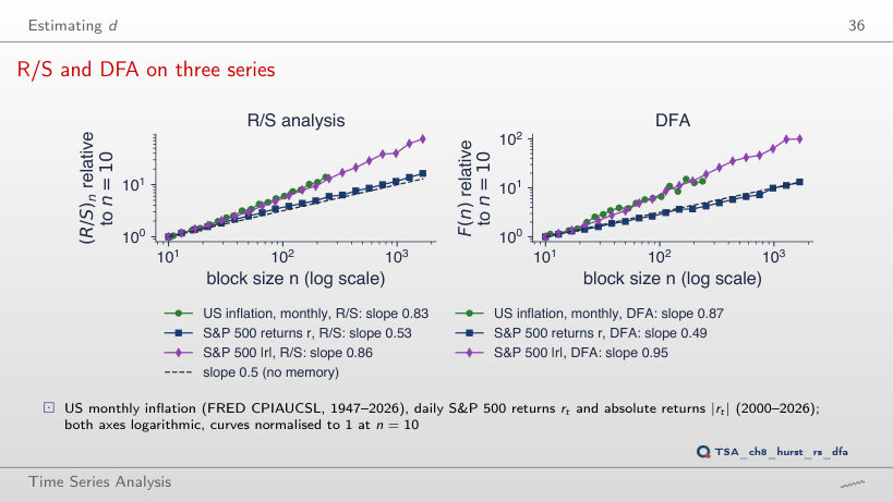
                                  Slide 36: R/S and DFA on three series
                                  Slide 36
                                    Question for the room Raise the smallest block to n = 60. What R/S slope do the S&P 500 absolute returns get?
                                    Answer

                                    0.92, against 0.86 with n from 10; returns stay at 0.53. In small blocks the day-to-day noise of |rt| dominates; the persistent part shows in large blocks.

                                    The periodogram and the GPH estimator
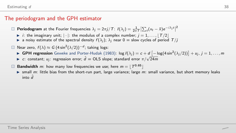
                                    Slide 38: The periodogram and the GPH estimator
                                    Slide 38

                                    Worked example

                                    \[\log I(\lambda_j)=c+d\,X_j+u_j,\quad X_j=-\log\!\big(4\sin^2(\lambda_j/2)\big),\quad \hat d=\frac{\sum_j(X_j-\bar X)(Y_j-\bar Y)}{\sum_j(X_j-\bar X)^2},\quad \mathrm{SE}=\frac{\pi}{\sqrt{24m}}\]
                                        Question for the room Romanian inflation with a = 0.5 (m = 16): what are d̂ and its SE?
                                        Answer

                                        d̂ = 0.56, SE 0.16. With fewer frequencies the estimate moves towards 0.5, and the standard error grows like 1/√m.

                                        GPH regressions: the Nile and Romanian inflation
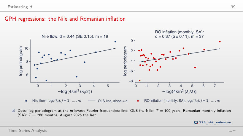
                                        Slide 39: GPH regressions: the Nile and Romanian inflation
                                        Slide 39
                                          Question for the room Set a = 0.8. What do GPH and local Whittle give for Romanian monthly inflation (m = 85)?
                                          Answer

                                          GPH 0.62 (SE 0.07), local Whittle 0.29 (SE 0.05). GPH works with log I, and the near-zero ordinates at the seasonal frequencies removed by the adjustment pull its slope up; local Whittle uses I itself and is not affected.

                                          Interpreting the GPH regressions
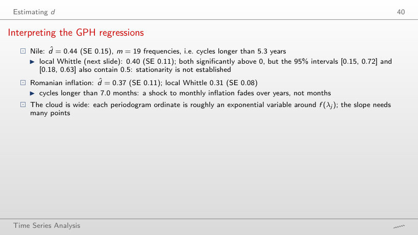
                                          Slide 40: Interpreting the GPH regressions
                                          Slide 40
                                            Question for the room Set a = 0.5. Does the GPH interval of the Nile still exclude 0?
                                            Answer

                                            No: d̂ = 0.39, SE 0.20, interval [−0.01, 0.79]. With m = 10 GPH no longer separates d from 0; local Whittle [0.15, 0.77] still does.

                                            The local Whittle estimator
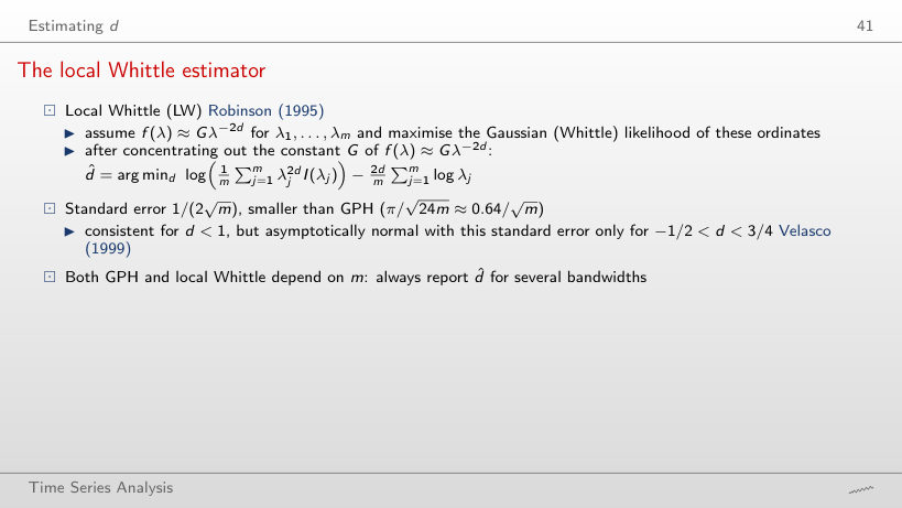
                                            Slide 41: The local Whittle estimator
                                            Slide 41

                                            Worked example

                                            \[R(d)=\log\Big(\frac1m\sum_{j=1}^m\lambda_j^{2d}I(\lambda_j)\Big)-\frac{2d}{m}\sum_{j=1}^m\log\lambda_j,\qquad \hat d=\arg\min_d R(d),\qquad \mathrm{SE}=\frac{1}{2\sqrt m}\]
                                                Question for the room Choose US unemployment (a = 0.65). Is the standard error 1/(2√m) valid?
                                                Answer

                                                No: d̂ = 0.91 > 3/4, outside the range of the normal approximation. The interval [0.80, 1.01] contains 1 anyway, so mean reversion is not established.

                                                Sensitivity to the bandwidth
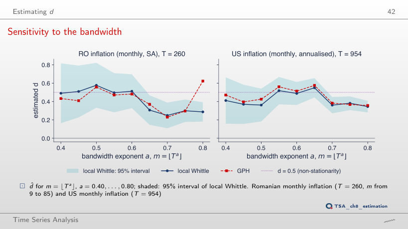
                                                Slide 42: Sensitivity to the bandwidth
                                                Slide 42
                                                  Question for the room End both samples in August 2019. Between which values does local Whittle move for the US and for Romania (T = 176)?
                                                  Answer

                                                  US: 0.35–0.54; Romania: 0.24–0.59. The conclusion of long memory stays, and the uncertainty of about ±0.15 is there without the years 2020–2026 too.

                                                  Monte Carlo: five estimators of d
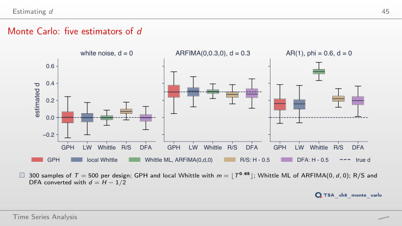
                                                  Slide 45: Monte Carlo: five estimators of d
                                                  Slide 45
                                                    Question for the room Use only the first 30 replications. Which estimator is the most precise at d = 0.3?
                                                    Answer

                                                    Whittle ML: standard deviation 0.033, against 0.076 (local Whittle) and 0.086 (GPH), the same order as with 300 replications (0.04, 0.08, 0.10).

                                                    Romanian inflation: ARMA or ARFIMA?
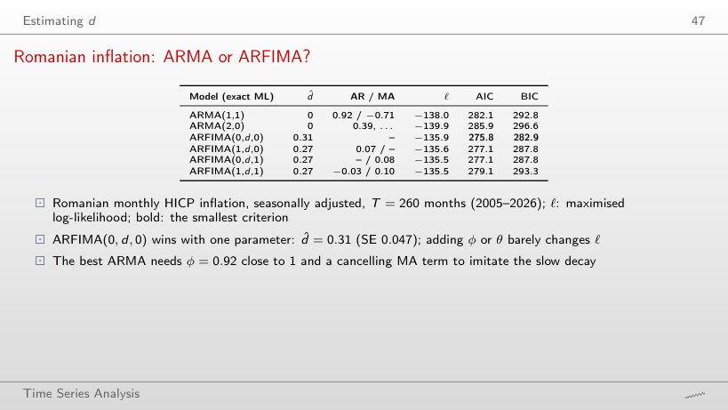
                                                    Slide 47: Romanian inflation: ARMA or ARFIMA?
                                                    Slide 47
                                                      Question for the room End the sample in December 2018 (T = 168). Which model has the smallest BIC, and what is d̂?
                                                      Answer

                                                      ARFIMA(0,d,0), with d̂ = 0.24: BIC 191.2 against 195.5 for ARMA(1,1). The conclusion of the lecture holds on the shorter sample too.

                                                      Romanian inflation: fitted autocorrelations
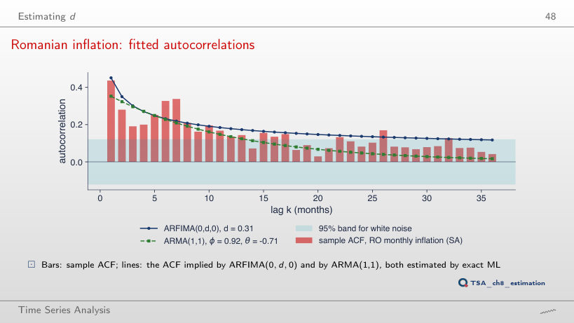
                                                      Slide 48: Romanian inflation: fitted autocorrelations
                                                      Slide 48
                                                        Question for the room Raise d by 0.14, to 0.45. How much does the log-likelihood fall, and is 2Δℓ above 3.84?
                                                        Answer

                                                        ℓ falls from −135.9 to −139.8; 2Δℓ = 7.8 > 3.84, so d = 0.45 is rejected at 5%. The ARFIMA curve becomes too high at lags 12 and 24 (0.65 and 0.60).

                                                        Long memory in twelve series
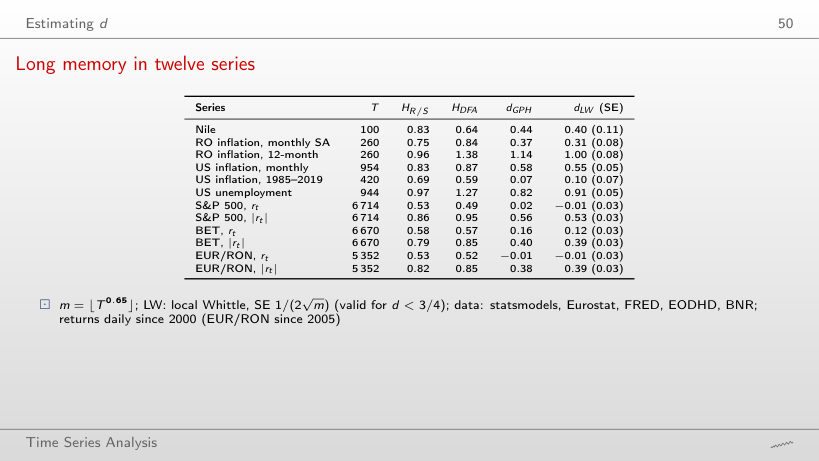
                                                        Slide 50: Long memory in twelve series
                                                        Slide 50
                                                          Question for the room Set a = 0.5 (m = 30 for US unemployment). Does the local Whittle interval still contain 1?
                                                          Answer

                                                          No: d̂ = 0.64, interval [0.46, 0.82], and the SE is valid (d̂ < 3/4). With a = 0.65 (m = 85): 0.91, [0.80, 1.01]. The verdict depends on the bandwidth.

                                                          Forecasting with ARFIMA

                                                          US inflation: ARFIMA and AR forecasts
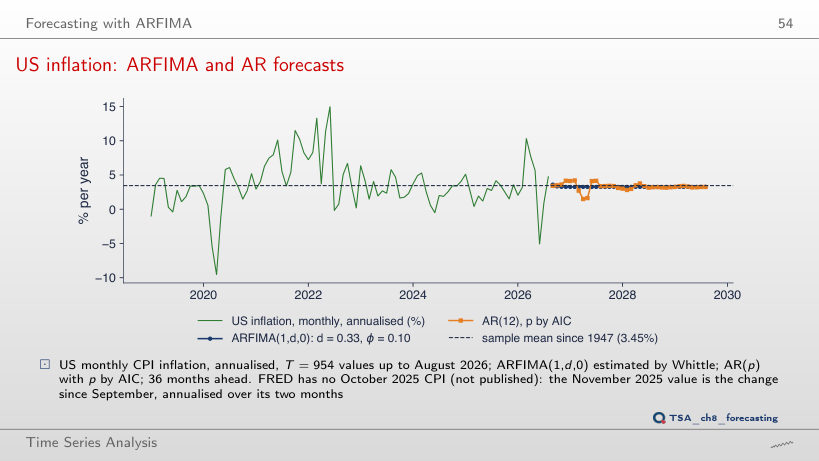
                                                          Slide 54: US inflation: ARFIMA and AR forecasts
                                                          Slide 54
                                                            Question for the room Move the origin to June 2022. Over the 36 months observed after it, which forecast has the smaller RMSE?
                                                            Answer

                                                            ARFIMA: 3.37 pp, against 4.02 pp for the AR(12). Both started high, but the AR(12) extended the 2022 peak (6.2% a year ahead, against 5.4%), and inflation fell faster.

                                                            Does long memory improve forecasts?
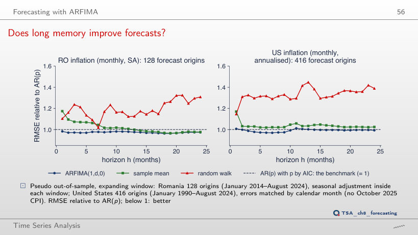
                                                            Slide 56: Does long memory improve forecasts?
                                                            Slide 56
                                                              Question for the room Drop the first 50% of the origins (Romania from May 2019). Does ARFIMA still beat the AR at every horizon in Romania?
                                                              Answer

                                                              No: the ratio is 1.038 at 1 month (the AR is better), 0.999 at 12 and 0.976 at 24. The gain remains at the long horizons only.

                                                              Interpreting the forecast comparison
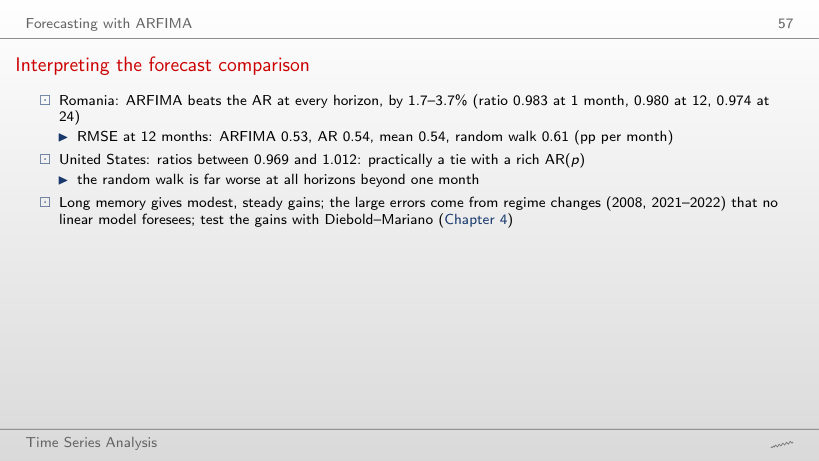
                                                              Slide 57: Interpreting the forecast comparison
                                                              Slide 57
                                                                Question for the room Drop the first 50% of the origins (Romania from May 2019). What are the 12-month RMSE of ARFIMA and of the random walk for Romania?
                                                                Answer

                                                                0.57 and 0.64 pp per month (against 0.53 and 0.61 on all origins): the random walk stays the worst.

                                                                Long memory in volatility

                                                                Returns, absolute and squared returns
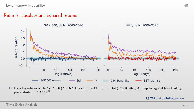
                                                                Slide 60: Returns, absolute and squared returns
                                                                Slide 60
                                                                  Question for the room Choose shuffled days. How many of the 250 autocorrelations of S&P 500 |rt| stay above the band, and what does local Whittle give?
                                                                  Answer

                                                                  6 of 250 (against 227), and local Whittle 0.00. The shuffle keeps the distribution and destroys the order: the memory lies in the sequence of calm and turbulent days.

                                                                  Monthly realised volatility: ARFIMA or ARMA?
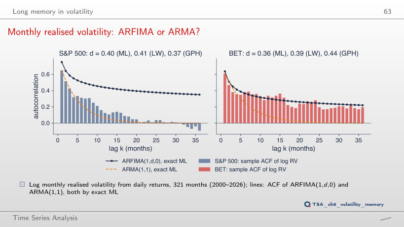
                                                                  Slide 63: Monthly realised volatility: ARFIMA or ARMA?
                                                                  Slide 63
                                                                    Question for the room Lower d by 0.30 (with φ fixed). By how much does the log-likelihood fall for the BET and for the S&P 500?
                                                                    Answer

                                                                    By 43.8 (BET) and 33.4 (S&P 500): both values are clearly rejected. For the BET the model ACF at lag 24 would be 0.004, against 0.28 in the sample.

                                                                    Interpreting realised volatility
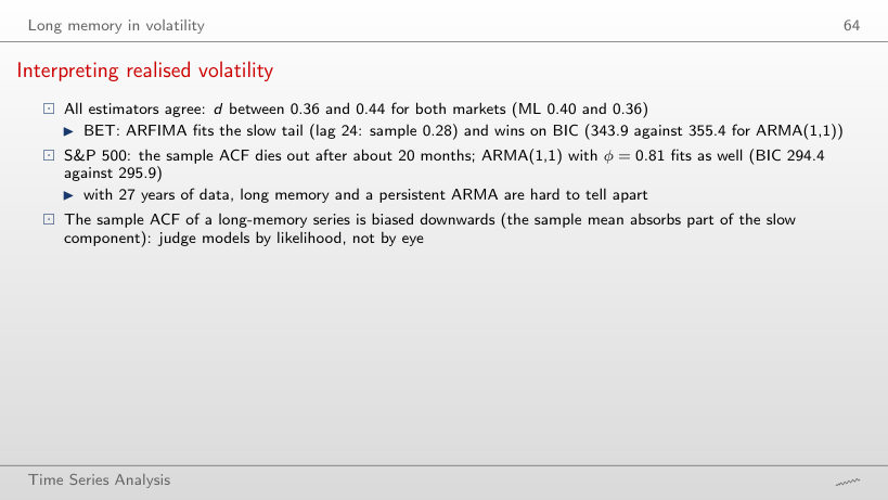
                                                                    Slide 64: Interpreting realised volatility
                                                                    Slide 64
                                                                      Question for the room Set a = 0.5 (m = 17). Between which values do the six estimates lie?
                                                                      Answer

                                                                      Between 0.36 (ML, BET) and 0.74 (GPH, BET), against 0.36–0.44 in the lecture. With few frequencies the semiparametric estimates scatter; ML does not depend on m.

                                                                      FIGARCH and HAR
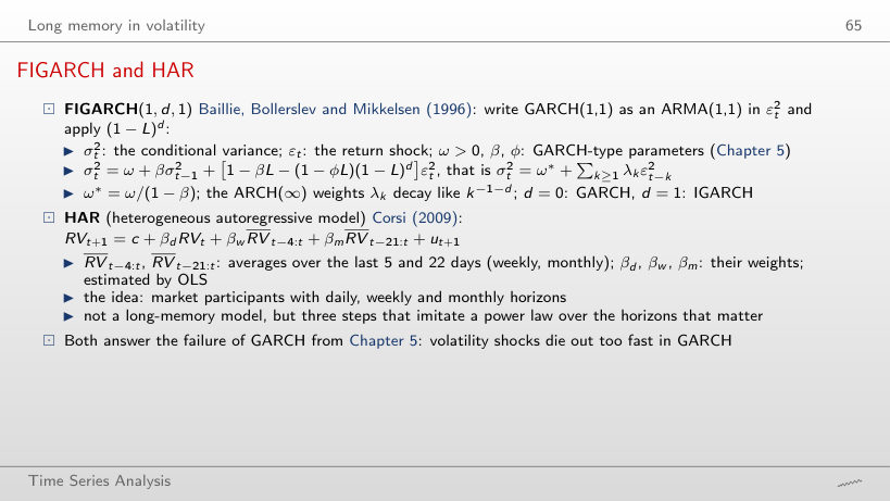
                                                                      Slide 65: FIGARCH and HAR
                                                                      Slide 65

                                                                      Worked example

                                                                      \[RV_{t+1}=c+\beta_d RV_t+\beta_w \overline{RV}_{t-4:t}+\beta_m \overline{RV}_{t-21:t}+u_{t+1},\quad w_1=\beta_d+\tfrac{\beta_w}{5}+\tfrac{\beta_m}{22},\ \ w_{2..5}=\tfrac{\beta_w}{5}+\tfrac{\beta_m}{22},\ \ w_{6..22}=\tfrac{\beta_m}{22}\]
                                                                          Question for the room End the sample in 2008. Which component has the largest coefficient, and what is β̂d?
                                                                          Answer

                                                                          The weekly one: β̂w = 0.62; β̂d = 0.10, half of 0.20 on 2000–2026.

                                                                          FIGARCH against GARCH; HAR against (1-L)^d
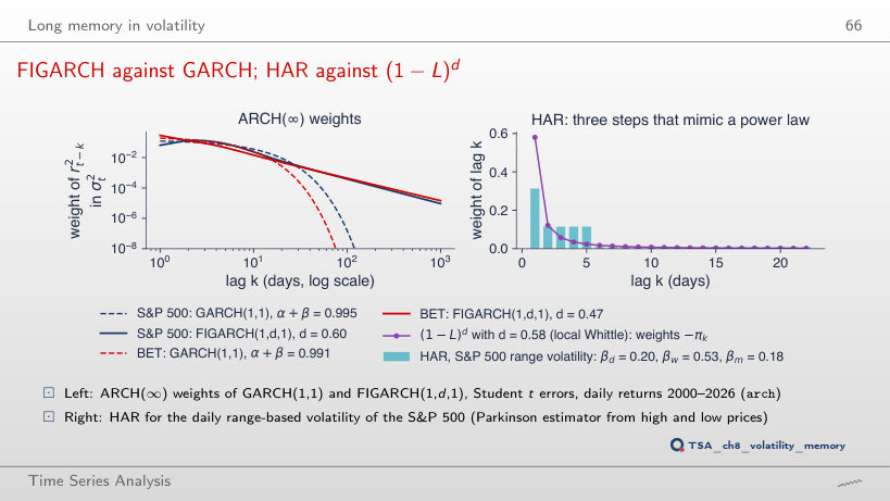
                                                                          Slide 66: FIGARCH against GARCH; HAR against (1-L)^d
                                                                          Slide 66
                                                                            Question for the room Move k to 500 days. What are the FIGARCH and GARCH weights of the S&P 500?
                                                                            Answer

                                                                            FIGARCH 2.9 · 10⁻⁵, GARCH 2.8 · 10⁻³¹. Even with α + β = 0.995 the GARCH weights fall exponentially; the FIGARCH weights fall like a power.

                                                                            Interpreting FIGARCH and HAR
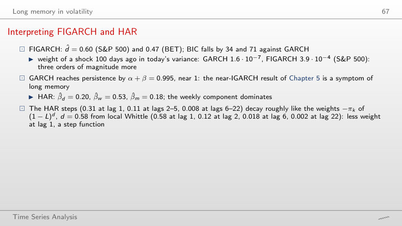
                                                                            Slide 67: Interpreting FIGARCH and HAR
                                                                            Slide 67
                                                                              Question for the room Raise d by 0.3 (to 0.88). How do the weights of (1 − L)d at lags 1 and 22 compare with HAR?
                                                                              Answer

                                                                              Lag 1: 0.88 against 0.31; lag 22: 0.0003 against 0.008. A larger d puts more weight on the first lag and less on the tail.

                                                                              Spurious long memory

                                                                              Apparent long memory in short-memory processes
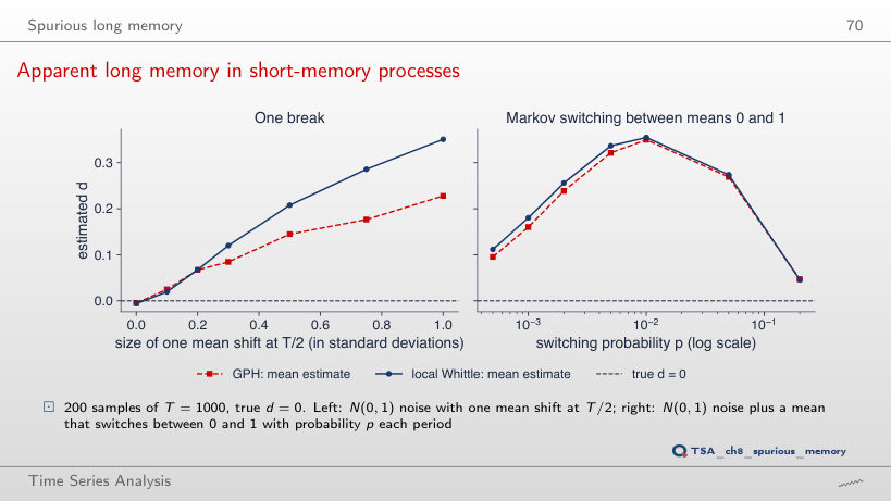
                                                                              Slide 70: Apparent long memory in short-memory processes
                                                                              Slide 70
                                                                                Question for the room Show the 5%–95% band. With a shift of one standard deviation, what is the 5% quantile of d̂ (local Whittle)?
                                                                                Answer

                                                                                0.31, above the 95% quantile without a shift (0.07): the distributions do not overlap, so every one of the 200 samples with a break shows “long memory”.

                                                                                The Nile in 1898: memory or a break?
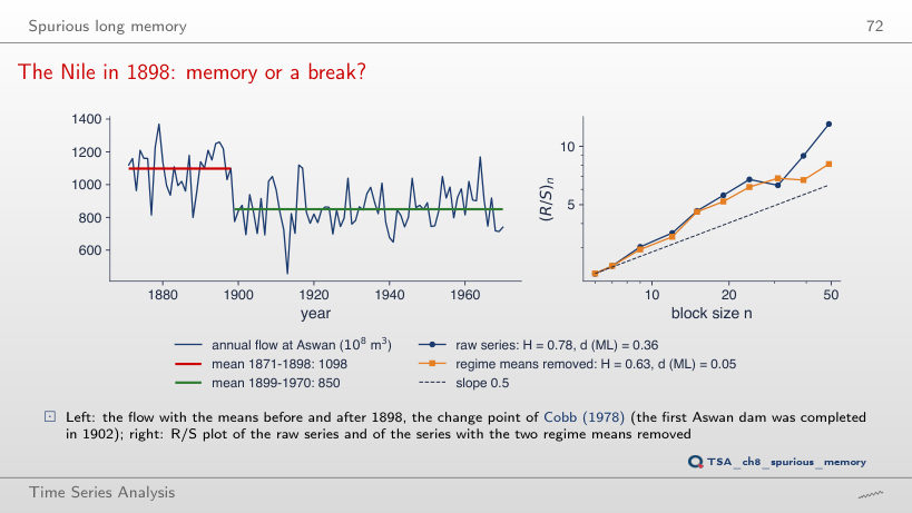
                                                                                Slide 72: The Nile in 1898: memory or a break?
                                                                                Slide 72
                                                                                  Question for the room Move the break to 1930. What d (exact ML) is left after removing the two means?
                                                                                  Answer

                                                                                  0.35, almost as in the raw series (0.36). A break placed in another year does not explain the memory; only the 1898 break brings it down to 0.05.

                                                                                  The stability of memory over time
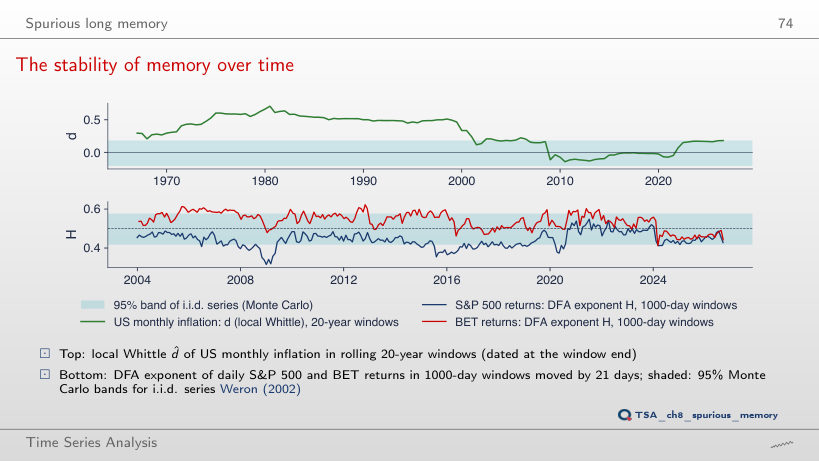
                                                                                  Slide 74: The stability of memory over time
                                                                                  Slide 74
                                                                                    Question for the room Halve the windows (10 years, 500 days). When and how high does d of US inflation peak?
                                                                                    Answer

                                                                                    0.64 in the window ending July 1974, against 0.71 in July 1980 with 20-year windows; the band of no memory widens to [−0.33, 0.25].

                                                                                    Nile flow at Aswan, 1871–1970 (statsmodels). Romanian HICP inflation, monthly and 12-month (Eurostat prc_hicp_minr, January 2005 – August 2026). US CPI inflation (FRED CPIAUCSL, February 1947 – August 2026) and the unemployment rate (FRED UNRATE, January 1948 – September 2026). The BNR EUR/RON reference rate and the daily S&P 500 and BET prices (data/market, up to 18 September 2026). The FRED, Eurostat and BNR series are read with the chapter’s loaders (downloaded on 4 November 2026) and cut at the end dates of the slides; they reproduce the numbers of the lecture exactly. The R/S, DFA, GPH and local Whittle estimators, the exact likelihood, the HAR regression and fractional differencing are recomputed in the browser; the simulations use the draws of the chapter’s seed, and the Monte Carlo estimates, the out-of-sample forecast errors, the Whittle ARFIMA(1,d,0) fits and the model tables are those of the chapter code. Variants that do not appear in the lecture (another sample, another bandwidth, another forecast origin, other windows, another d) are extra runs of the chapter code with the same data and seed.