Chapter 0: Introduction: components and exponential smoothing
Daniel Traian PELE
Bucharest University of Economic Studies IDA Institute Digital Assets Blockchain Research Center AI4EFin Artificial Intelligence for Energy Finance Romanian Academy, Institute for Economic Forecasting MSCA Digital Finance
Almost all of the phenomena of economic life, like many other processes, social, meteorological, and others, occur in sequences of rising and falling movements, like waves.
A time series is a sequence of observations of one variable, ordered in time. Unlike a sample of independent units, the order of the observations carries information: this quarter resembles the previous one, this January resembles last January, and a shock to the exchange rate persists for years. The chapter asks three questions that run through the whole course: which patterns repeat in economic, financial, energy and climate data, how these patterns can be separated from one another, and how a forecast is produced and judged.
The running example is Romanian real GDP, observed every quarter from 1995 Q1 to 2026 Q2. Three patterns overlap in one series. The economy grew about 2.3 times between 1995 and 2025, a trend. Within each year the first quarter lies about 23.8% below the trend and the fourth about 20.7% above it, a seasonal pattern. Annual GDP fell by 5.5% in 2009 and by 3.6% in 2020, interruptions of the trend that come at no fixed date. Slutzky (1937) showed that wave-like movements of this kind need not have a periodic cause: they can arise from the summation of purely random shocks. A chart alone therefore cannot tell which mechanism produced a wave.
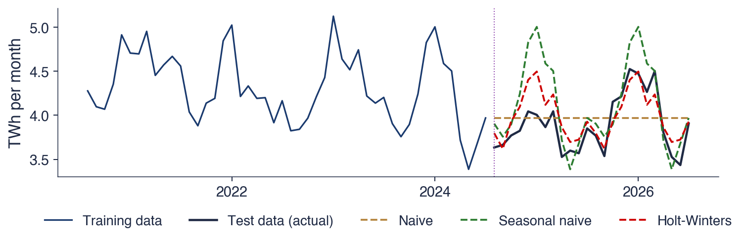
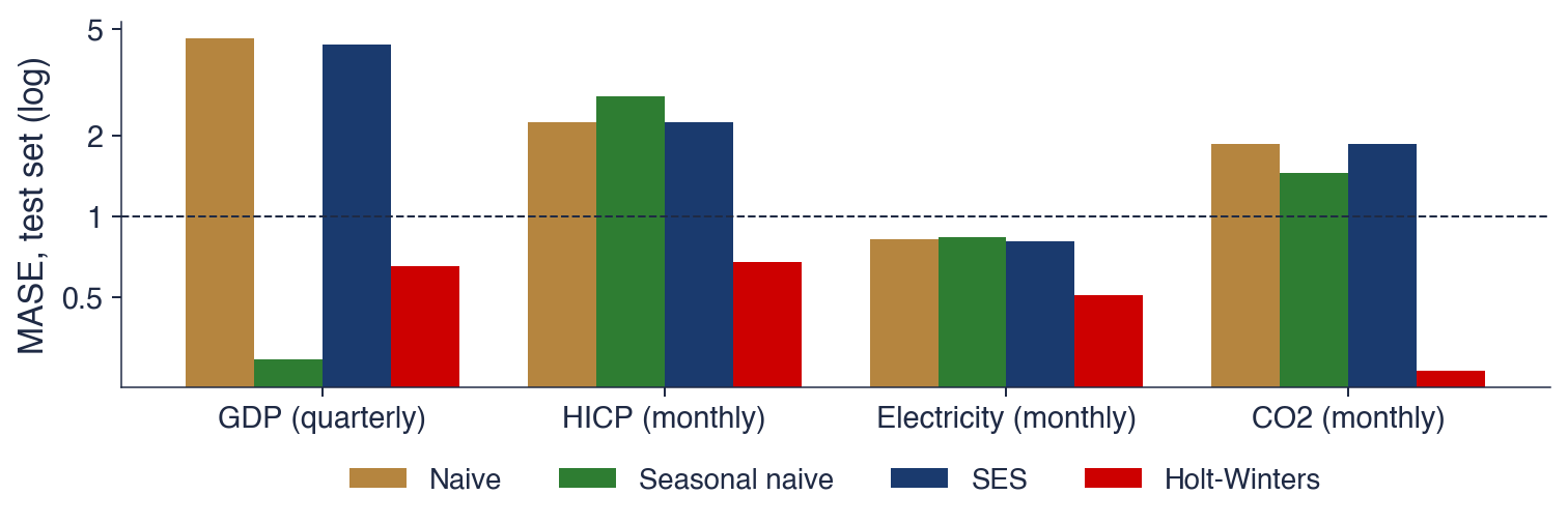
The methods of this chapter are descriptive and need no probability model: the decomposition of a series into trend, seasonality and remainder, moving averages, growth rates, the sample autocorrelation function, exponential smoothing, and the evaluation of forecasts against simple benchmarks on data the method has not seen. On Romanian electricity generation, the Holt–Winters method reaches a mean absolute error of 0.17 TWh per month on a two-year test set, against 0.28 TWh for the naive forecast. On GDP, the seasonal naive forecast, which simply repeats last year's quarter, beats Holt–Winters. The probability models that explain these results start in Chapter 1.
Romanian real GDP, quarterly, 1995 Q1 to 2026 Q2, chain-linked volumes at 2010 prices, in billion EUR: the series as measured (blue) and the series adjusted for seasonal and calendar effects (red). Trend, seasonality and recessions are visible in one chart.
What you will be able to do
Recognise trend, seasonality, cycle and remainder in a chart, and choose between an additive and a multiplicative decomposition.
Compute growth rates, a centred moving average, seasonal factors and a sample autocorrelation.
Produce naive, seasonal naive, simple exponential smoothing and Holt–Winters forecasts.
Evaluate forecasts on a test set with MAE, RMSE, MAPE and MASE.
Chapter plan
Course organisationThe programme, the assessment, the textbooks, the map of the chapters, the seminars, the team project and the AI policy.
What a time series isDefinition, the three kinds of data, the goals of the analysis, flows and stocks, adjusted data.
Time series on real dataSix series: GDP, inflation, EUR/RON, stock indices, electricity and CO2, each read for its patterns.
A short historySunspots, Yule and Slutsky, Kolmogorov and Wiener, Box and Jenkins.
Components and decompositionTrend, seasonality, cycle and remainder; moving averages, classical decomposition and STL.
ConclusionsKey ideas, self-assessment and the link to Chapter 1.
Course organisation
This section describes how the course is built: the programme it belongs to, the assessment, the textbooks, the order of the chapters, the materials available for each chapter, the format of the seminars, the team project and the rules for using AI tools. The conventions introduced here, such as the reproducible chart folders and the declaration of AI use, apply to every later chapter.
The chapter is organised around three questions. The first is what a time series is and where one meets it; the answer is a definition, a distinction from other kinds of data, and six real series from economics, finance, energy and climate. The second is which patterns repeat in such data; the answer is the decomposition into trend, seasonality, cycle and remainder. The third is how a series is forecast and how one knows whether the forecast is good; the answer is a set of simple forecasting methods and a protocol for measuring their errors on data the method has not seen.
Part I builds the vocabulary: the organisation of the course, the examples, a short history of the field and the components of a series. Part II introduces the formal tools: notation, transformations, the sample autocorrelation function, exponential smoothing, and forecast evaluation. Each learning outcome on the slide corresponds to a computation that the chapter carries out twice, once by hand on a few numbers and once on a real series. Seminar 0 takes place before this lecture and practises the first tools on data; the lecture then explains why the tools work and when they fail.
In brief
Guiding questions
what is a time series, and where do we meet one?
which patterns repeat in economic, financial, energy and climate data?
how do we forecast a series, and how do we know the forecast is good?
Part I
how the course works
time series on real data and a short history
components: trend, seasonality, cycle, noise
Part II
notation, transformations and a first look at the ACF
exponential smoothing; forecasts and their evaluation
tools, and the possible contribution of AI
Learning outcomes: after this chapter you can
explain how the course is organised and graded
recognise trend, seasonality, cycle and noise in a chart
compute growth rates, a moving average and a sample autocorrelation
produce naive and exponential smoothing forecasts
evaluate forecasts on a test set with MAE, RMSE and MASE
Seminar 0 comes before this lecture and practises the first tools on data
Time Series Analysis is a course of the Bachelor's programmes Economic Informatics and Economic Cybernetics, in the second semester of the third year, at the Faculty of Cybernetics, Statistics and Economic Informatics (CSIE) of the Bucharest University of Economic Studies (ASE). It carries 4 ECTS credits and is taught in the academic year 2026/2027 by Prof. Daniel Traian Pele.
The course assumes three prerequisites. Probability and statistics provide the language of random variables, expectations and tests, which Chapter 1 extends from one random variable to a sequence of them, a stochastic process. Econometrics, in particular the linear regression model, is used directly: many time-series models are regressions of a variable on its own past values, and the course explains which classical results survive when the observations are dependent. Python is the computing environment of all examples. The course website collects the slides, the seminars, the notebooks, the Quantlets and the quizzes of every chapter.
In brief
Programme
Bachelor's programmes Economic Informatics and Economic Cybernetics, year 3, semester 2
Faculty of Cybernetics, Statistics and Economic Informatics (CSIE), ASE Bucharest
4 ECTS credits; 2 hours of lecture and 1 hour of seminar a week; academic year 2026/2027
The final grade has three components. The written exam counts for 70% and tests three skills: reading and interpreting the output of time-series software, carrying out short derivations, and choosing a suitable model for a given series. It covers the lectures and seminars of Chapters 0 to 10 and the review in Chapter 15. The team project counts for 20%: two to four students analyse and forecast real time series with the methods of the course and present the work as a GitHub repository, a short report, a presentation and an oral defence. Attendance at lectures and seminars and the chapter quizzes together count for the remaining 10%.
The three components add up to 100%. The quizzes, one per chapter on the course website, are taken with the ASE Google account, and the name and score are recorded for the grade. Each quiz draws 20 questions from a bank of 24 and explains every answer, so it also shows which parts of a chapter need another reading before the exam.
In brief
Written exam: 70%
reading and interpreting software output, short derivations, choosing a model for a given series
covers the lectures and seminars of Chapters 0–10 and 15
Team project: 20%
2–4 students analyse and forecast real time series with the methods of the course
a GitHub repository, a short report, a presentation and an oral defence
Attendance and quizzes: 10%
lectures and seminars
one quiz per chapter on the website: 20 questions drawn from a bank of 24, each answer explained
taken with the ASE account; name and score are recorded for the grade
The main textbook is Huang & Petukhina (2022),Applied Time Series Analysis and Forecasting with Python. The chapters of the course follow its order: components and smoothing, stationarity, ARMA models, ARIMA models, seasonality, volatility and multivariate models. The free companion is Hyndman & Athanasopoulos (2021),Forecasting: Principles and Practice, available online in its third edition. It is the reference for the topics of this chapter: decomposition, exponential smoothing and the evaluation of forecasts.
Two books provide the theory. Brockwell & Davis (2016) give a rigorous introduction to stationary processes, ARMA models and forecasting, with proofs. Hamilton (1994) is the standard reference of time-series econometrics, with full treatments of unit roots, vector autoregressions and cointegration, the topics of the later chapters. The companion is the place to look for how a method is used; the two theoretical books are the place to look for why it works.
The course has sixteen chapters. Chapters 0 to 5 study one series at a time: this introduction, stochastic processes and stationarity, ARMA models, unit roots and ARIMA models, seasonality and forecasting with SARIMA, TBATS and Prophet, and conditional volatility with ARCH and GARCH. Chapters 6 and 7 study several series together: vector autoregressions (VAR) with Granger causality, and cointegration with the vector error correction model (VECM). Chapters 8 to 10 extend the framework: long memory and ARFIMA models, machine learning for time series, and state space models with the Kalman filter and Markov switching. Chapter 15 reviews the course and prepares the exam.
The order goes from the dynamics of one series, first its mean and then its variance, to the joint dynamics of several series. Chapters 11 to 14, marked with an asterisk, are self-study: foundation models for time series, spectral analysis, speculative bubbles with LPPL (log-periodic power law) models, and multivariate GARCH models. They have shorter materials and a quiz, without a compulsory seminar, and they are not part of the exam.
In brief
No.
Chapter
0
Introduction: components and exponential smoothing
1
Stochastic processes and stationarity
2
ARMA models
3
Unit roots and ARIMA models
4
Seasonality and forecasting: SARIMA, TBATS, Prophet
5
Conditional volatility: ARCH and GARCH
6
VAR models and Granger causality
7
Cointegration and VECM
No.
Chapter
8
Long memory and ARFIMA
9
Machine learning for time series
10
State space models, Kalman filter and Markov switching
11
Foundation models for time series\(^*\)
12
Spectral analysis\(^*\)
13
Speculative bubbles: LPPL models\(^*\)
14
Multivariate GARCH models\(^*\)
15
Review and exam preparation
Univariate models (0–5), several series (6, 7), extensions (8–10), review (15)
Self-study, marked \(^*\): Chapters 11–14 (shorter materials and a quiz, no compulsory seminar)
Every chapter has the same set of materials: lecture and seminar slides in Romanian and in English, a lecture notebook and a seminar notebook in Python that open in Google Colab with one click, and a quiz of 20 questions. The notebooks repeat the computations of the slides on the same data, so that every result can be reproduced and modified.
Every chart of the slides has a Quantlet: a public folder with the code that produces it, a short description file and the chart itself. The icon under each chart opens its Quantlet on GitHub. The data come from public sources and are read directly in the code: Eurostat, the National Institute of Statistics (INS), the National Bank of Romania (BNR) and FRED (Federal Reserve Economic Data, the database of the Federal Reserve Bank of St. Louis). Daily market data come from EODHD (EOD Historical Data) and are stored in the course repository up to 18 September 2026, so that the market charts can be reproduced exactly.
In brief
For every chapter
lecture and seminar slides, in Romanian and in English
a lecture notebook and a seminar notebook (Python), opened in Google Colab with one click
a quiz of 20 questions
Quantlets: every chart has a public folder with its code, a description file (Metainfo.txt) and the chart
the icon under each chart opens its Quantlet on GitHub
Data: public sources, read directly in the code
Eurostat, INS (National Institute of Statistics), BNR (National Bank of Romania), FRED (Federal Reserve Bank of St. Louis)
daily market data from EODHD (EOD Historical Data), saved in the course repository until 18 September 2026
Each seminar has three parts. Part A consists of short calculations on paper, such as a moving average or an autocorrelation computed from a few numbers. Part B works with real data, and every task ends with an interpretation question, because a number without an interpretation is not an answer. Part C contains an open idea that can grow into a project, and the critique of an answer produced by an AI assistant.
The exercises are of two kinds. A solved exercise, marked [Solved], has its full solution in the slides and in the notebook and serves as a model. A proposed exercise, marked [Proposed], is solved by the students, and the solution is discussed in class. Nothing is handed in: the seminar is practice for the exam and for the project. Since each seminar precedes its lecture, it is written as a self-contained introduction to the tools of the chapter.
In brief
Three parts
A: short calculations on paper; B: real data, each task ending with an interpretation question; C: an open idea and the critique of an AI answer
Two kinds of exercises
[Solved]: full solution in the slides and in the notebook, a model to follow
[Proposed]: you solve it; the solution is discussed in class
Nothing is handed in: the seminar is practice for the exam and for the project
The project starts from one question about real time series, chosen by the team: a forecasting question, such as the electricity demand of next winter, or a modelling question, such as the response of inflation to the exchange rate. The methods are those of the course: decomposition and smoothing, ARIMA and SARIMA, GARCH, VAR or VECM, Granger causality, impulse responses and forecast evaluation. Romanian data from INS, BNR, Eurostat and the Bucharest Stock Exchange (BVB) are encouraged.
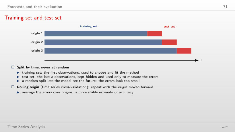
The deliverables are a GitHub repository whose code reproduces every number and every chart, a short report, a presentation and a file that declares the use of AI tools. Four criteria determine the grade: a clear question, correct methods with their diagnostic checks, an honest out-of-sample evaluation, and the oral defence, in which each member explains the code and the results. An honest out-of-sample evaluation means that the forecasts are scored on observations that played no role in choosing or estimating the model; the section on forecast evaluation shows how this is done.
In brief
Question: one forecasting or modelling question on real time series, chosen by the team
Methods: those of the course
decomposition and smoothing, ARIMA and SARIMA, GARCH, VAR or VECM, Granger causality, impulse responses, forecast evaluation
Romanian data (INS, BNR, Eurostat, BVB) are encouraged
Deliverables
a GitHub repository whose code reproduces every number and every chart
a short report, a presentation and the file AI_USE.md
Grading
a clear question, correct methods and diagnostics, an honest out-of-sample evaluation
oral defence: each member explains the code and the results
AI tools are allowed and must be declared. Here AI means assistants based on a large language model (LLM) that write text and code. Every use is recorded in a declaration file: the tool, the prompt, what was kept and what was corrected. The declaration makes the work reproducible and shows where the student's own judgement entered.
The student remains responsible for every number and every reference. The typical errors of AI assistants are invented references, wrong formulas, and code that runs but computes something other than what it claims. Two checks follow: every reference is opened through its DOI (Digital Object Identifier) and its title is compared with the citation, and every number is recomputed with the student's own code. The oral defence applies the same principle to the code: a line that the student cannot explain does not count as the student's work. The section on AI lists the time-series errors that AI-generated code makes most often.
In brief
AI tools are allowed and must be declared
AI: artificial intelligence; here, assistants based on an LLM (large language model) that write text and code
every use goes into AI_USE.md: the tool, the prompt, what was kept, what was corrected
You are responsible for every number and every reference
typical AI errors: invented references, wrong formulas, code that runs but computes something else
every reference: open its DOI (Digital Object Identifier) and check the title
every number: recompute it with your own code
Oral defence
a line of code you cannot explain does not count as your work
Section summary
The course combines a written exam on Chapters 0 to 10 and 15 with a team project on real data, attendance and quizzes. Its materials are bilingual, reproducible and open: every chart has its code, every chapter has notebooks and a quiz. AI tools may be used, provided that every use is declared and every number and reference is checked. The next section defines the object of the course.
What a time series is
This section defines a time series, sets the notation, and explains what distinguishes time series from the other kinds of data met in statistics and econometrics. It then lists the goals of time-series analysis and three practical distinctions that matter before any computation: the frequency of the data, flows versus stocks, and adjusted versus unadjusted series.
A time series is a set of observations of one variable, recorded at successive moments and ordered in time. It is written \(y_1, y_2, \ldots, y_T\), where \(t\) is the time index (a quarter, a month, a day) and \(T\) is the number of observations. The frequency is the number of observations per year: 4 for quarterly data, 12 for monthly data, and about 252 for daily market data, since exchanges trade only on working days.
The example is Romanian real GDP, in billion EUR at 2010 prices: 38.7 in 2024 Q1, 45.6 in Q2, 52.8 in Q3, 59.2 in Q4, and 38.9 in 2025 Q1. Read in order, the five numbers tell a story: output rises through the year, peaks in the fourth quarter and falls back at the start of the next year to roughly the level of a year earlier. Shuffled, the same five numbers keep their mean and their variance, but the story disappears. This is the sense in which the order carries information.
The figures are in real terms, at the prices of 2010, so their changes measure changes in volume and not in prices. In the language of Chapter 1, the observed series is one realisation of a stochastic process: \(T\) observations, but a single path of the process, which can never be observed twice.
In brief
Time series: observations of one variable, recorded at successive moments and ordered in time
Notation: \(y_1, y_2, \ldots, y_T\)
\(t\): the time index (quarter, month, day); \(T\): the number of observations
frequency: the number of observations per year (4 quarterly, 12 monthly, about 252 for trading days)
Example: Romanian real GDP, quarterly, billion EUR at 2010 prices
Statistical data come in three structures. Cross-section data observe many units at one moment, such as the GDP of the 27 countries of the European Union (EU) in 2025. A time series observes one unit at many moments, such as Romanian GDP in every quarter since 1995. Panel data observe many units at many moments, such as the GDP of the 27 EU countries in every quarter. The methods of this course are those of the second row; panels combine both dimensions.
What changes in a time series is the dependence between observations. In a random sample of countries, knowing the GDP of one country says nothing about the next one drawn. In a time series, this quarter resembles the previous one. This dependence is the information used to forecast: if consecutive values were independent, the past would contain nothing about the future beyond the overall mean. It also means that the classical formulas derived for independent samples must be adapted. The standard error of a sample mean, \(s/\sqrt{T}\), assumes independent observations; with positively dependent observations, \(T\) values contain less information than \(T\) independent ones, and the formula understates the uncertainty. The corrections are developed from Chapter 1 onwards.
In brief
Type
Structure
Example
Cross-section
many units, one moment
GDP of the 27 EU countries in 2025
Time series
one unit, many moments
Romanian GDP, every quarter since 1995
Panel
many units, many moments
GDP of the 27 EU countries, every quarter
What changes in a time series
observations are not independent: this quarter resembles the previous one
this dependence is the information we use to forecast
the classical formulas for independent samples (standard errors, tests) must be adapted
The table pairs four fields with their series and a typical question. In economics, GDP, inflation and unemployment are followed by governments and central banks, and a typical question is where inflation will be in a year. In finance, exchange rates, stock indices and interest rates are the objects, and a typical question is how risky the BET index will be tomorrow. In energy, the production and consumption of electricity and its prices are planned months ahead. In climate science, the concentration of CO2 and temperatures are measured to separate a long-run rise from the seasonal swing.
The questions differ in kind. Some ask for the level of a variable at a horizon, some for its risk, some for a quantity to be planned, and some for a trend hidden under a seasonal pattern. What they have in common is that decisions depend on the answer. A central bank sets its interest rate on its inflation forecast, because monetary policy acts with a delay; a grid operator plans production on its demand forecast, because electricity cannot be stored cheaply at scale. A biased forecast leads to a wrong decision even when the model fits the past well.
In brief
Field
Series
Typical question
Economics
GDP, inflation, unemployment
Where will inflation be in a year?
Finance
exchange rates, stock indices, interest rates
How risky is the BET tomorrow?
Energy
electricity production and consumption, prices
How much electricity is needed next January?
Climate
CO2 concentration, temperatures
How fast does CO2 rise, beyond the seasonal swing?
Decisions depend on forecasts: the central bank sets the interest rate on its inflation forecast; the grid operator plans production on its demand forecast
Time-series analysis pursues four goals. Description summarises a series by its trend, seasonality, cycles and unusual observations, through charts, decomposition and autocorrelations; this is the subject of this chapter and of Chapter 1. Modelling proposes a probability model that could have produced the data, such as the ARMA, ARIMA and GARCH models of Chapters 2 to 5. A model turns a description into a statement about uncertainty: it says not only what the series did but how it could have behaved.
Forecasting predicts values not yet observed, together with their uncertainty, and is the goal that runs through the whole course. Explanation and control study how one series responds to another, for example how inflation responds to a change in the interest rate, with VAR models, Granger causality and cointegration in Chapters 6 and 7. Box & Jenkins (1970) framed the same goals as a cycle of four steps applied to a single series: identify a model, estimate it, check it, and forecast with it.
A flow is measured over a period; a stock is measured at a moment. The GDP of a quarter and the electricity produced in a month are flows: they accumulate over the period, and the flow of a year is the sum of the flows of its quarters. The exchange rate on a given day, the concentration of CO2 and the level of a stock index are stocks: they describe a state at a point in time, and adding them over time has no meaning.
The distinction decides how the frequency of a series is changed. To go from monthly to quarterly data, flows are summed, while stocks are averaged or represented by their last value. The monthly EUR/RON series used later in the chapter is the average of the daily rates of each month.
Statistical offices publish many series in two versions. The seasonally adjusted series removes the regular pattern within the year and the calendar effects, such as the number of working days in a quarter. The unadjusted series is what was measured; the adjusted series is an estimate, which is revised when new observations arrive and the seasonal pattern is re-estimated. For Romanian GDP in 2026 Q2, the unadjusted value is 45.9 billion EUR and the adjusted value 48.8 billion EUR: the second quarter is seasonally weak, so adjustment raises it. A model of the seasonal pattern itself needs the unadjusted series.
In brief
Flow: measured over a period; stock: measured at a moment
flows: GDP of a quarter, electricity produced in a month; they add up over time
stocks: exchange rate on a day, CO2 concentration, an index level; we average them, we do not add them
Changing the frequency
monthly to quarterly: the sum for flows, the average or the last value for stocks
Seasonally adjusted data
the statistical office removes the regular within-year pattern and the calendar effects (number of working days)
the unadjusted series is what was measured; the adjusted one is an estimate, revised when new data arrive
The chapter uses six series, chosen so that each displays a different combination of patterns. Romanian real GDP comes from Eurostat, quarterly, from 1995 Q1 to 2026 Q2. The Romanian Harmonised Index of Consumer Prices (HICP), computed with the same method in every EU country, comes from Eurostat, monthly, from 1996 to August 2026. Romanian electricity generation comes from Eurostat, monthly, from January 2008 to July 2026. The EUR/RON exchange rate is the daily reference rate of the BNR, from 2005 to 2026.
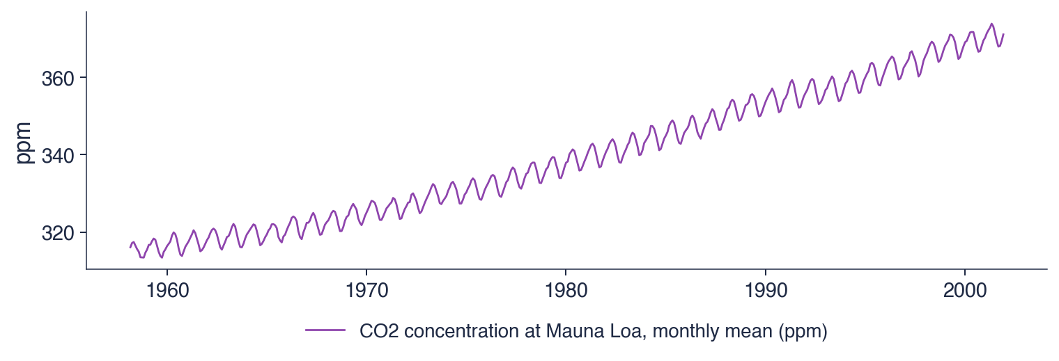
The two stock indices are daily, from 2000 to 2026: the BET, the reference index of the Bucharest Stock Exchange (BVB), and the S&P 500, which covers 500 large companies in the United States. The CO2 concentration at Mauna Loa is the classic data set distributed with statsmodels, the Python library for statistical models used throughout the course; its weekly measurements are averaged by month, from 1958 to 2001. The sources are public, so every number in the chapter can be recomputed.
In brief
Series
Source
Frequency
Sample
Romanian real GDP
Eurostat
quarterly
1995 Q1 – 2026 Q2
Romanian HICP (consumer prices)
Eurostat
monthly
1996 – August 2026
Electricity generation, Romania
Eurostat
monthly
January 2008 – July 2026
EUR/RON
BNR reference rate
daily
2005 – 2026
BET, S&P 500
EODHD
daily
2000 – 2026
CO2 at Mauna Loa
statsmodels data set
weekly, averaged monthly
1958 – 2001
HICP: Harmonised Index of Consumer Prices, computed with the same method in every EU country
BET: the reference index of the BVB (Bucharest Stock Exchange); S&P 500: 500 large US companies
statsmodels: the Python library for statistical models used throughout the course
A time series is one variable observed over time, and the order of its observations carries information. Consecutive observations depend on one another, and this dependence is both the basis of forecasting and the reason why the formulas for independent samples must be adapted.
Time-series analysis describes, models, forecasts and explains. Before any computation three facts about the data must be settled: the frequency, whether the variable is a flow, which adds up over time, or a stock, which is averaged, and whether the series is the measured one or a seasonally adjusted estimate.
In brief
A time series is one variable observed over time; the order of the observations carries information
Consecutive observations depend on each other: this is the basis of forecasting
Goals: describe, model, forecast, explain
Flows add up, stocks are averaged; adjusted series are estimates
Section summary
A time series differs from a cross-section through the dependence between its observations, which makes forecasting possible and changes the inference. Its frequency, its nature as a flow or a stock, and its adjustment status determine how it can be aggregated and modelled. The next section reads six real series and identifies the patterns that the rest of the chapter formalises.
Time series on real data
This section reads six real series, from Romanian GDP to atmospheric CO2. Each series is shown as a chart, and the following slide interprets the chart: which patterns are present, how large they are, and which events explain the unusual observations. The six readings prepare the vocabulary of the section on components: trend, seasonality, cycle and noise.
The chart shows Romanian real GDP every quarter from 1995 Q1 to 2026 Q2, in billion EUR. The values are chain-linked volumes at 2010 prices: each year's growth is computed at the prices of the previous year, and the growth rates are linked into one index expressed in the prices of 2010. Changes in the series therefore measure changes in production, not in prices.
Two lines are drawn. The blue line is the series as measured, which zigzags within every year. The red line is the series adjusted by Eurostat for seasonal and calendar effects; it runs through the middle of the zigzag and shows the underlying movement. The vertical distance between the two lines in a given quarter is the seasonal effect of that quarter.
In brief
Quarterly, 1995 Q1 – 2026 Q2, chain-linked volumes at 2010 prices (billion EUR); blue: as measured; red: seasonally and calendar adjusted (Eurostat)
The trend is the dominant feature: the Romanian economy grew about 2.3 times from 1995 to 2025, an average real growth of 2.8% a year. The two numbers are linked by compounding, since a growth of 2.8% a year over thirty years multiplies the level by \(1.028^{30} \approx 2.3\).
The seasonal pattern is equally clear: in every year the first quarter lies far below the fourth. Winter brings less construction and agricultural work, while autumn brings the harvest and the activity of the end of the year. The swing grows with the level of GDP: in 2024 the fourth quarter exceeded the first by about 20 billion EUR (59.2 against 38.7), and since the seasonal effects are percentages of the level, the gap in billion EUR was smaller when the economy was smaller. A swing proportional to the level is the mark of a multiplicative pattern, which the section on components estimates.
Recessions interrupt the trend at irregular dates: annual GDP fell by 5.5% in 2009, during the global financial crisis, and by 3.6% in 2020, during the COVID-19 pandemic. These are the cyclical movements of the series. The last observation, 2026 Q2, is 45.9 billion EUR unadjusted and 48.8 billion EUR adjusted.
In brief
Trend: the economy grew about 2.3 times from 1995 to 2025
an average real growth of 2.8% a year
Seasonality: every year, Q1 is far below Q4
winter: less construction and agriculture; autumn: the harvest and year-end activity
the swing grows with the level of GDP: a multiplicative pattern
Cycle: recessions interrupt the trend
annual GDP fell by 5.5% in 2009 (global financial crisis) and by 3.6% in 2020 (COVID-19 pandemic)
Last value, 2026 Q2: 45.9 billion EUR unadjusted, 48.8 adjusted
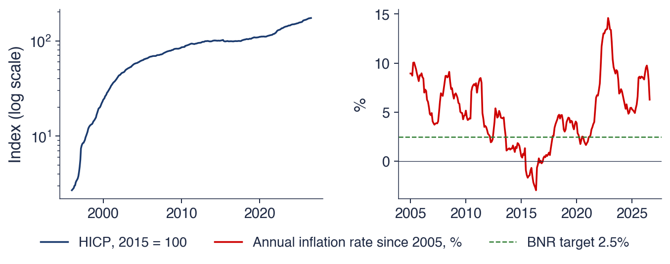
The left panel shows the HICP, with 2015 = 100, on a logarithmic scale. On such a scale equal vertical distances correspond to equal percentage changes, so the slope of the line is the inflation rate: a steep line means fast inflation, a flat line stable prices. The right panel shows the annual inflation rate since 2005,
where \(P_t\) is the HICP in month \(t\), together with the inflation target of the BNR, 2.5%.
The two panels are two transformations of the same data. The index is the level of prices, the rate its percentage change over twelve months. Most of the analysis in later chapters is done on such transformed series, because the rate has a stable mean and the level does not.
In brief
Left: HICP, 2015 = 100, log scale; right: annual inflation rate \(100\,(P_t/P_{t-12} - 1)\) since 2005, against the BNR target of 2.5%; \(P_t\): the HICP in month \(t\)
The level and the rate tell different stories. The price index almost never falls, so its trend is the inflation accumulated since the base year. The inflation rate rises and falls, and it is the series a central bank targets. Four episodes mark the history of the rate: 178% in June 1997, after the liberalisation of prices that year; −3.0% in May 2016, after the cuts in value added tax (VAT) of 2015 and 2016; 14.6% in November 2022, during the energy price shock; and 6.3% in August 2026, the last observation.
The negative rate of 2016 shows that a tax change can move the measured inflation rate for exactly twelve months: the lower price level enters the numerator of \(P_t/P_{t-12}\) at once, and leaves the comparison a year later. The same mechanism explains why a rate over twelve months removes the seasonal pattern but reacts with a delay. Comparing each month with the same month a year earlier cancels the regular within-year movements, but the rate reflects the whole past year, so a change in the price trend appears in it only gradually.
In brief
Level and rate tell different stories
the price index almost never falls: its trend is the accumulated inflation
the inflation rate rises and falls: it is the series the central bank targets
Episodes
June 1997: 178%, after the price liberalisation of 1997
May 2016: \(-\)3.0%, after the VAT cuts of 2015–2016
November 2022: 14.6%, the energy price shock
August 2026: 6.3%
A rate over 12 months removes the seasonal pattern but reacts with a delay: it reflects the whole past year
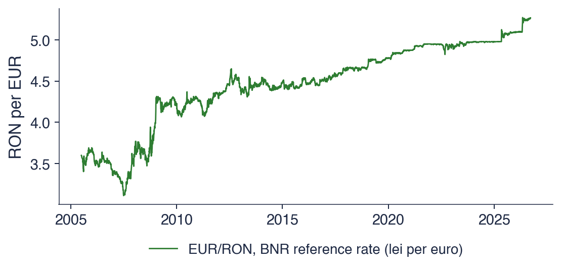
The chart shows the number of lei paid for one euro, according to the daily reference rate of the BNR, on every working day from 4 July 2005 to 18 September 2026, a total of 5,353 observations. The reference rate is fixed once a day from quotes of the interbank market, so the series is a stock: the value at a moment, not the sum over a period.
The series has no seasonal zigzag, unlike GDP and electricity. Its movement consists of long periods in which the rate changes little, interrupted by short episodes of fast depreciation of the leu. The interpretation slide quantifies both.
In brief
Lei per euro, every working day from 4 July 2005 to 18 September 2026 (5 353 observations)
The rate rose from 3.5986 lei at the start of the sample to 5.2644 at the end, with a minimum of 3.1112 on 2 July 2007. The rise did not follow a fixed shape, such as a straight line: long calm periods alternate with jumps, in the autumn of 2008, in 2012 and in 2025. A trend of this kind, built from the accumulation of shocks that are never reversed, is called a stochastic trend; it is the subject of Chapters 1 and 3.
The series has no seasonality, and an argument from market behaviour explains why. If the euro were predictably cheaper every spring, traders would buy it in spring and sell it later in the year; their purchases would raise the spring price until the pattern disappeared. Predictable patterns in the prices of freely traded assets tend to be removed by the trading they invite.
The daily changes are small: the standard deviation of the daily log change is 0.28%. The largest move, 2.93% on 3 October 2008, is about ten standard deviations, an event that a Normal distribution with the same standard deviation would practically never produce. Rare large moves of this kind are typical of financial series and return in Chapter 5.
In brief
A trend without a fixed shape
from 3.5986 to 5.2644 lei; lowest value 3.1112 on 2 July 2007
long calm periods, interrupted by jumps (autumn 2008, 2012, 2025)
No seasonality
if the euro were predictably cheaper every spring, traders would buy it in spring and the pattern would disappear
Daily changes
standard deviation of the daily log change: 0.28%; the largest move: 2.93% on 3 October 2008
A trend like this one, built from accumulated shocks, is called a stochastic trend (Chapters 1 and 3)
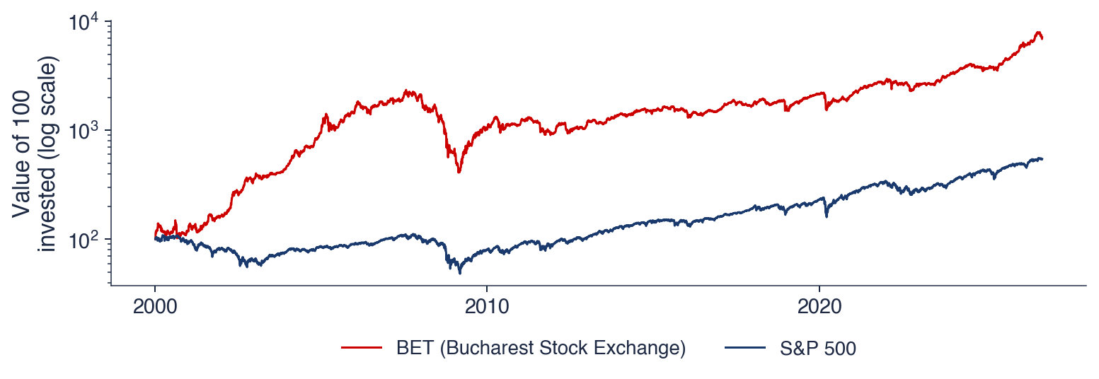
The chart shows the value of 100 units invested on 5 January 2000 in each of the two indices, computed from closing prices. The vertical axis is logarithmic, so equal vertical distances are equal percentage changes: a fall from 200 to 100 and a fall from 2,000 to 1,000 have the same height.
Rebasing both indices to 100 on the same day makes their paths comparable even though their levels differ by orders of magnitude. The chart answers a simple question: what became of the same amount invested in the Romanian and in the US stock market at the start of 2000.
In brief
Value of 100 invested on 5 January 2000, closing prices, log scale: equal vertical distances are equal percentage changes
Both indices grew over the long run, with deep falls. An amount invested in the BET was multiplied by about 71, an amount invested in the S&P 500 by about 5.5. Both are price indices, without dividends, so the total return of an investor was higher. In 2008 and 2009 the BET lost more than three quarters of its value; a loss of 75% requires a gain of 300% to return to the previous level, which is why the recovery took years.
The logarithmic scale is necessary for such a series. On a linear scale the early years look flat and the recent moves look huge, because a change of 10% is ten times larger in index points when the index is ten times higher. The logarithm turns constant percentage growth into a straight line, so the slope of the chart can be read as a growth rate in every period.
The prices of traded assets are hard to forecast, for the same reason as the exchange rate: predictable price moves are removed by trading. Their risk, the size of future moves regardless of sign, is much easier to forecast, as Chapter 5 shows with GARCH models.
In brief
Long-run growth with deep falls
100 invested grew about 71-fold in the BET and 5.5-fold in the S&P 500 (price indices, without dividends)
2008–2009: the BET lost more than three quarters of its value; it took years to recover
Why the log scale
on a linear scale, the early years look flat and recent moves look huge
the logarithm turns constant percentage growth into a straight line
Prices of traded assets are hard to forecast; their risk is easier to forecast (Chapter 5)
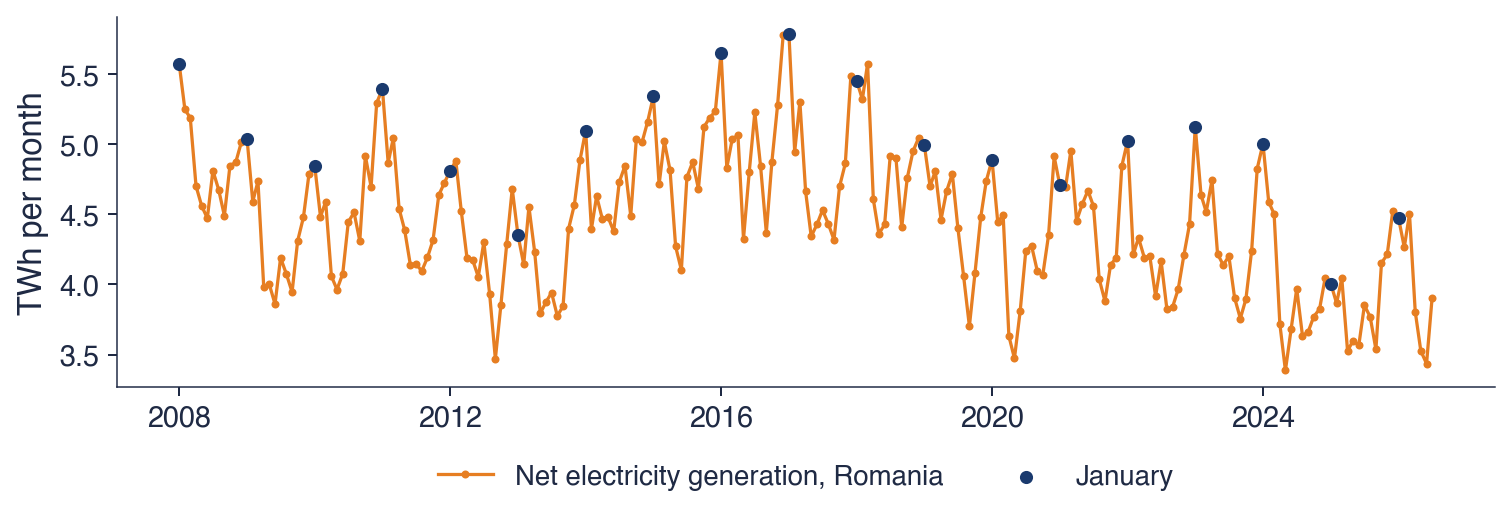
The chart shows the net electricity generation of Romania, in TWh per month, from January 2008 to July 2026, according to Eurostat. Net generation is the electricity delivered by power plants after their own consumption. The dots mark January of each year, so that the seasonal peak can be followed from one winter to the next.
The series is a flow: the generation of a year is the sum of its months. Three features are visible at once: a regular yearly wave, a level that drifts down over the sample, and years whose wave is higher or lower than usual.
In brief
Net electricity generation, TWh per month, January 2008 – July 2026 (Eurostat); dots: January of each year
The seasonal pattern is strong. The month with the highest average generation is January, with 5.03 TWh, and the month with the lowest is September, with 4.06 TWh; the ratio of the two averages is 1.24, so a typical January generates about a quarter more than a typical September. The cause is the winter demand for heating and lighting.
The level falls over the sample: the generation of the year was 58.5 TWh in 2008 and 46.7 TWh in 2025. More imports and a lower industrial demand explain the decline. A forecasting method for this series must therefore combine a falling level with a stable winter peak, which is what the Holt–Winters method of the section on smoothing does.
Some years are irregular: dry years reduce hydropower generation, and mild winters reduce demand. These deviations do not repeat with a fixed period and form the remainder of the series. The units are the terawatt-hour, TWh, equal to \(10^{12}\) watt-hours, and the gigawatt-hour, GWh, equal to \(10^{9}\) watt-hours.
In brief
Strong seasonality
highest average month: January (5.03 TWh); lowest: September (4.06 TWh)
winter demand for heating and lighting; the ratio of the two averages is 1.24
A falling level
58.5 TWh in 2008, 46.7 TWh in 2025: more imports, less industrial demand
Irregular years
dry years reduce hydropower; mild winters reduce demand
In 1958 Charles David Keeling started measuring the concentration of CO2 (carbon dioxide) at Mauna Loa, in Hawaii, a site far from local sources of pollution (Keeling, 1960). The measurements have continued since then and form the longest continuous record of atmospheric CO2. The unit is ppm, parts per million: molecules of CO2 per million molecules of dry air.
The series contains two patterns. The trend rises because emissions from fossil fuels accumulate in the atmosphere. The yearly wave comes from the vegetation of the Northern Hemisphere, which holds most of the land surface: plants absorb CO2 in summer through photosynthesis and release it in winter, when leaves decay. The Keeling curve is the textbook example of a series in which trend and seasonality are both clear and almost free of noise.
In brief
1958: Charles David Keeling starts measuring CO2 at Mauna Loa, Hawaii, far from local sources (Keeling (1960))
the longest continuous record of atmospheric CO2
Two patterns in one series
a rising trend: fossil fuel emissions accumulate
a yearly wave: plants of the Northern Hemisphere absorb CO2 in summer and release it in winter
ppm: parts per million, molecules of CO2 per million molecules of dry air
The chart shows the monthly averages of the weekly measurements from March 1958 to December 2001, a total of 526 months. This is the classic data set distributed with statsmodels, which ends in 2001; its four decades are long enough to show how both the trend and the seasonal wave evolve.
The chart is read in two scales at once. Over decades, the line rises steadily. Within each year, a regular wave goes up and down. The section on components separates the two with the STL method.
In brief
Monthly averages of the weekly measurements, March 1958 – December 2001 (526 months; the classic data set of statsmodels)
The trend rises from 316.1 ppm in March 1958 to 371.0 ppm in December 2001, on average 1.26 ppm a year. The slope itself increases over time: the curve bends upwards, so the concentration rises faster at the end of the sample than at the start. A straight line fitted to the whole sample would underestimate the recent slope.
The seasonal wave is regular, with a size of a few ppm. It keeps roughly its size while the level rises, which is the mark of an additive pattern, in contrast to GDP. The series has almost no noise, because it is a careful physical measurement and not an economic statistic built from surveys or a price formed by trading. A smooth series with a clear trend and season is the easiest case for decomposition and smoothing, and the CO2 series is therefore the reference case in the rest of the chapter.
In brief
Trend: from 316.1 to 371.0 ppm
on average 1.26 ppm a year; the slope itself increases over time
Seasonality: a regular yearly wave of a few ppm
the wave keeps roughly its size while the level rises: an additive pattern
Almost no noise
a careful physical measurement, unlike GDP or exchange rates
A smooth series with a clear trend and season: the easiest case for decomposition and smoothing
The table summarises the six readings by the four components. Unadjusted GDP has a rising trend, a strong multiplicative season, cycles in the form of recessions and little noise. The inflation rate falls after 1997, its season is removed by the twelve-month rate, its cycles are shocks, and its noise is medium. EUR/RON has a stochastic trend, no season, no cycle and medium noise. The BET rises with crashes, has no season, shows booms and busts, and has large noise. Electricity falls, with a strong winter peak and medium noise. CO2 rises at an accelerating pace, with a regular additive season and very small noise.
Question for the room. Which of these series would you forecast most accurately one year ahead? Answer. CO2, because its trend is smooth, its season stable and its noise small; the BET is the hardest, because it has neither a season to repeat nor a trend that can be extrapolated, and its noise is large. The ranking anticipates the results of the section on forecast evaluation, where Holt–Winters forecasts CO2 with a MASE of 0.26, the smallest error of the chapter.
In brief
Series
Trend
Season
Cycle
Noise
GDP (unadjusted)
up
strong, multiplicative
recessions
small
Inflation rate
down after 1997
removed by the 12-month rate
shocks
medium
EUR/RON
stochastic
–
–
medium
BET
up, with crashes
–
booms and busts
large
Electricity
down
strong, winter peak
–
medium
CO2
up, accelerating
regular, additive
–
very small
Question for the room: which of these series would you forecast most accurately one year ahead?
Answer: CO2: a smooth trend and a stable season, little noise; the BET is the hardest: no season and large noise
Section summary
The six series show the four components in different proportions. GDP and electricity are dominated by trend and season; EUR/RON and the BET by accumulated shocks, with no season; CO2 by a smooth trend and a regular wave; the inflation rate by episodes. Seasonal swings may be proportional to the level, as for GDP, or constant, as for CO2. The next section shows how the first models of such waves were found.
A short history
The methods of time-series analysis grew from a few problems, each solved by a person whose name is still attached to a model. This section follows them from the sunspot numbers of the nineteenth century to the method of Box and Jenkins in 1970 and places the later developments on one time line. The history is not decoration: each step introduced an idea that the course uses directly.
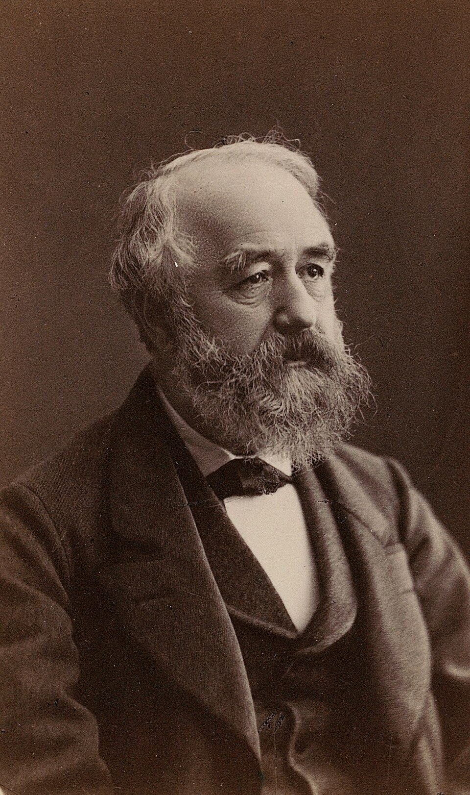
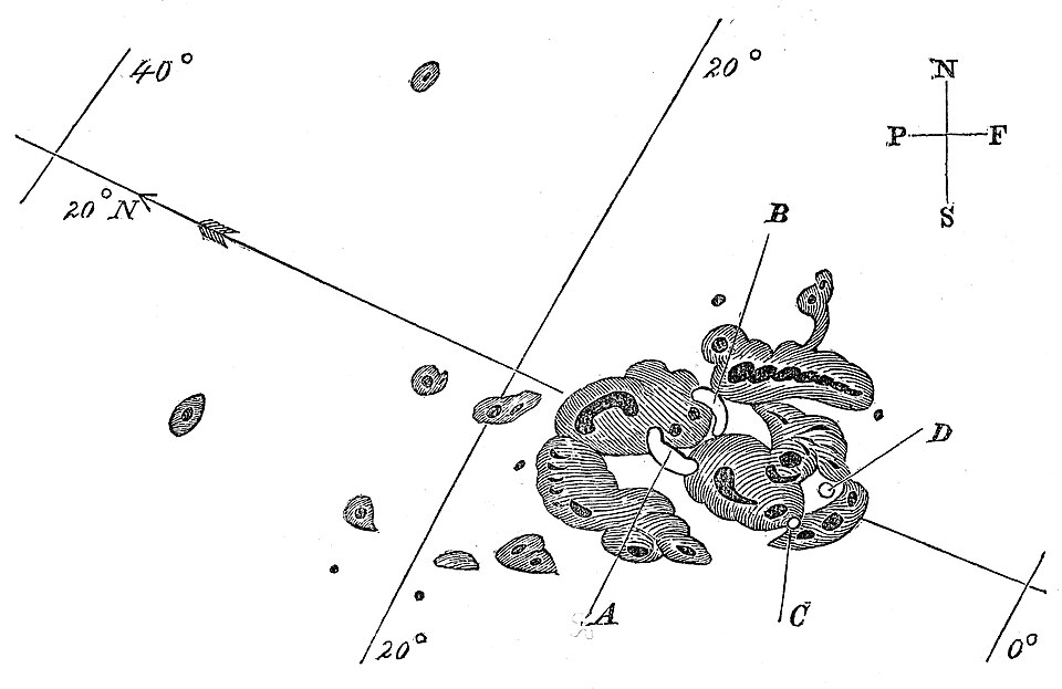
In 1848 the Swiss astronomer Rudolf Wolf defined a daily index of solar activity based on the number of sunspots and reconstructed it back to 1749. These are the Wolf numbers, later continued by his successor Alfred Wolfer. The drawing by Richard Carrington, from 1 September 1859, shows the kind of observation from which the index is built.
The series rises and falls in waves of about 11 years, but neither the length nor the height of the waves is constant. This raised the question that shaped the early history of the field: is the series a hidden periodic signal, a sum of sine waves, plus measurement noise, or is it produced by a different mechanism? If it were a sum of sine waves, the period would be fixed and the waves could be forecast far ahead; the drift of the period in the data argues against it.
Yule (1926) studied what he called nonsense correlations between time series. Two series with no causal link but with trends can show a correlation close to 1, simply because both rise or fall over the sample. His example was the share of marriages celebrated by the Church of England and the mortality rate in England and Wales, which moved together over decades. The problem reappears in Chapter 3 as spurious regression and in Chapter 7, where cointegration distinguishes a genuine long-run relation from a coincidence of trends.
Yule (1927) explained Wolfer's sunspot numbers by their own past instead of by hidden sine waves:
where \(y_t\) is the sunspot number in year \(t\),\(\phi_1\) and \(\phi_2\) are coefficients estimated from the data, and \(\varepsilon_t\) are random disturbances. Without disturbances, suitable coefficients make the equation oscillate with a damped wave whose length and damping are set by \(\phi_1\) and \(\phi_2\). With disturbances, each shock pushes the wave and shifts its phase, so the period drifts, as in the data. This was the first autoregressive model, AR(2), studied in Chapter 2.
In brief
1926: nonsense correlations between time series (Yule (1926))
two unrelated series with trends can show a correlation close to 1
his example: the share of Church of England marriages and the mortality rate in England and Wales
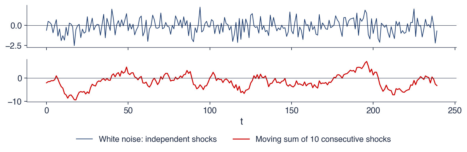
Eugen Slutsky published his paper in Moscow in 1927; the English version appeared ten years later as The summation of random causes as the source of cyclic processes(Slutzky, 1937). His experiment starts from independent random numbers \(\varepsilon_1, \varepsilon_2, \ldots\), taken from the digits of a lottery draw, and replaces each one by the sum of the last ten:
The resulting series looks like the business cycles of the economic statistics of his time, with expansions and contractions of irregular length. In modern terms \(y_t\) is a moving-average process of order 9, MA(9), one of the two building blocks of the models of Chapter 2. Yule found waves in a series that depends on its own past; Slutsky found them in a series that depends on past shocks.
The chart repeats the experiment with a computer. The top panel shows 240 independent shocks drawn from the standard Normal distribution: a series without any structure, in which each value is unrelated to the others. The bottom panel shows the moving sum of 10 consecutive shocks, computed exactly as in Slutsky's construction.
The contrast between the two panels is the point of the experiment. The top panel jumps erratically around zero. The bottom panel moves in smooth waves that stay above or below zero for many periods, although nothing periodic was put into it. The only operation between the two panels is a summation.
In brief
Top: 240 independent shocks with the standard Normal distribution; bottom: the moving sum of 10 consecutive shocks
No cycle was put in, yet waves appear. The moving sum crosses zero upwards 16 times in 240 periods, so the average wave lasts about 15 periods, but the individual waves have irregular lengths. The reason is the overlap between neighbouring values: \(y_t\) and \(y_{t-1}\) share 9 of their 10 shocks. If the shocks have variance \(\sigma^2\), the covariance of \(y_t\) and \(y_{t-k}\) is \((10-k)\sigma^2\) for \(k < 10\) and zero beyond, so the autocorrelation is
\[\rho_k = \frac{10-k}{10}, \qquad k = 0, 1, \ldots, 9,\]
equal to 0.9 at lag 1 and declining linearly to zero at lag 10. Strong correlation between neighbours makes the series move slowly, and slow movements around zero look like waves.
The experiment teaches two lessons. A cycle in a chart is not proof of a periodic cause: summed shocks produce cycles too. Smoothing with moving averages, the tool of the section on components, can itself create apparent cycles in data that had none, so cycles found in smoothed data must be interpreted with care. Together, Yule's autoregression and Slutsky's moving average are the two building blocks of the ARMA models.
In brief
No cycle was put in, yet waves appear
the moving sum crosses zero upwards 16 times in 240 periods: waves of irregular length
neighbouring values share 9 of their 10 shocks, so they are strongly correlated
Implications
a cycle in a chart is not proof of a periodic cause
smoothing (moving averages) can create apparent cycles: be careful with smoothed data
Yule (AR) and Slutsky (MA) gave the two building blocks of the ARMA models
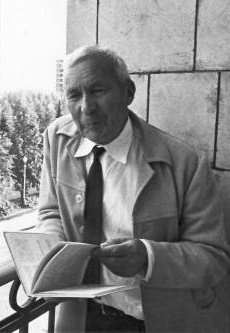
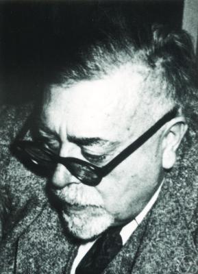
In 1941 Andrei Kolmogorov published the theory of interpolation and extrapolation of stationary sequences (Kolmogorov, 1941). Independently, Norbert Wiener developed the same theory for continuous signals in a classified report of 1942, written for anti-aircraft fire control, where a gun must aim at the position an aircraft will have when the shell arrives; the report was published in 1949 (Wiener, 1949).
Both answered the same question: which weighted sum of past values forecasts the future value with the smallest mean squared error? For a stationary series, the optimal weights depend only on the autocovariances of the series, the quantities estimated by the sample autocorrelation function of the notation section. Their solution, known as the Wiener filter, is the ancestor of the Kalman filter of Chapter 10, which computes the same optimal forecast recursively, one observation at a time.
1942 (classified report), 1949: the Wiener filter, developed for anti-aircraft fire control (Wiener (1949))
Both answer: which weighted sum of past values forecasts the future with the smallest mean squared error? The ancestor of the Kalman filter (Chapter 10)
In 1970 George Box and Gwilym Jenkins published Time Series Analysis: Forecasting and Control(Box & Jenkins, 1970). The theory of Kolmogorov and Wiener assumed that the autocovariances were known; Box and Jenkins turned it into a procedure that starts from data. The Box–Jenkins cycle has four steps: identify a model from the charts and the autocorrelation function (ACF), estimate its parameters, check whether the residuals behave like unpredictable noise, and forecast only when the checks pass. If the checks fail, the cycle returns to identification.
The ARIMA models and their seasonal version, SARIMA, come from this book and are studied in Chapters 2 to 4. Box summarised the attitude of the method in a sentence often quoted: all models are wrong, but some are useful. A model is judged by whether its residuals contain no remaining structure and by how well it forecasts, not by whether it is literally true.
In brief
1970: George Box and Gwilym Jenkins publish Time Series Analysis: Forecasting and Control (Box & Jenkins (1970))
The Box–Jenkins cycle
identify: choose a model from charts and the ACF
estimate: fit its parameters
check: are the residuals unpredictable noise?
forecast: only when the checks pass
ARIMA models and their seasonal version SARIMA come from this book (Chapters 2–4)
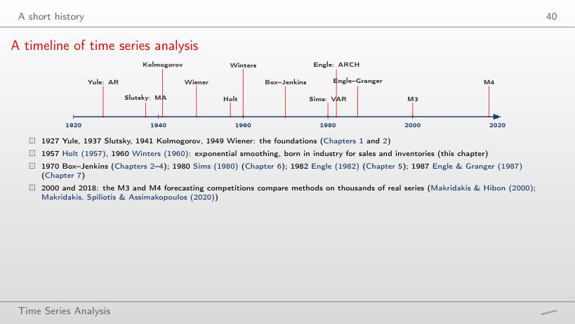
The time line places the main contributions on one axis. Between 1927 and 1949, Yule, Slutsky, Kolmogorov and Wiener laid the foundations: autoregression, moving averages and optimal linear prediction, the material of Chapters 1 and 2. In 1957 and 1960, Holt (1957) and Winters (1960) introduced exponential smoothing, born in industry to forecast sales and inventories; it is the subject of this chapter.
From 1970 the field branched out. Box and Jenkins gave the ARIMA methodology of Chapters 2 to 4; Sims (1980) proposed vector autoregressions as an alternative to large structural models (Chapter 6); Engle (1982) modelled time-varying variance with ARCH (Chapter 5); Engle & Granger (1987) formalised cointegration and error correction (Chapter 7). The M3 and M4 forecasting competitions, reported by Makridakis & Hibon (2000) and by Makridakis, Spiliotis & Assimakopoulos (2020), compared methods on thousands of real series, and both found that simple methods are hard to beat.
Two ideas from the 1920s underlie the whole course: a series can be explained by its own past (Yule), and summed random shocks produce waves without any periodic cause (Slutsky). Kolmogorov and Wiener turned dependence into optimal forecasts, and Box and Jenkins into a practical cycle of identification, estimation, checking and forecasting. The next section returns to the descriptive tools that precede any model: the components of a series and their estimation.
Components and decomposition
A decomposition writes a series as a combination of components that have a clear interpretation: a slowly changing trend, a seasonal pattern that repeats every year, and a remainder. This section defines the components, distinguishes cycle from seasonality, introduces the additive and multiplicative forms, and builds the classical decomposition from centred moving averages. It applies the method to Romanian GDP and then presents STL, a more flexible decomposition, on the CO2 series.
A series is described by four components. The trend \(T_t\) is the long-run movement of the level, such as the growth of GDP or the rise of CO2; it may change direction, but only slowly. The seasonality \(S_t\) is a pattern that repeats with a fixed and known period \(m\):\(m = 4\) for quarterly data, \(m = 12\) for monthly data, \(m = 7\) for daily data with a weekly pattern.
The cycle \(C_t\) consists of rises and falls without a fixed period, usually longer than a year; business cycles, with expansions and recessions of 2 to 10 years, are the standard example. Because its length is not known in advance, a cycle cannot be separated from the trend by a fixed rule, and decomposition methods usually merge the two into a single trend-cycle component. The remainder \(R_t\), also called the irregular component or noise, is what is left after trend and season are removed. It should look unpredictable: if the remainder still shows a pattern, such as a regular wave or a slow drift, the decomposition has missed something.
In brief
Trend\(T_t\): the long-run movement of the level
GDP growth, the rise of CO2; it can change direction slowly
Seasonality\(S_t\): a pattern that repeats with a fixed, known period\(m\)
\(m = 4\) for quarterly data, \(m = 12\) for monthly data, \(m = 7\) for daily data with a weekly pattern
Cycle\(C_t\): rises and falls without a fixed period, usually longer than a year
business cycles: expansions and recessions of 2–10 years; usually merged with the trend into a trend-cycle
Remainder\(R_t\) (irregular component, noise): what is left
it should look unpredictable; if it does not, the decomposition missed something
Question for the room. Electricity generation is high every January. Is this a cycle or seasonality? Answer. Seasonality: the period is fixed, twelve months, and it is known in advance. A recession, in contrast, arrives at an unknown moment and lasts an unknown time, and that is a cycle.
The distinction matters for forecasting. Seasonality can be forecast years ahead: next January will again be high, and its size relative to the trend can be estimated from past Januaries. Cycles are hard to forecast because their timing changes, as Slutsky's experiment showed. The sunspot series illustrates the difference: its waves of about 11 years are a cycle and not a season, because their length varies from one wave to the next, and no calendar announces the next peak.
In brief
Question for the room: electricity generation is high every January
is this a cycle or seasonality?
Answer: seasonality: the period is fixed (12 months) and known in advance
a recession arrives at an unknown moment and lasts an unknown time: that is a cycle
Why the difference matters
seasonality can be forecast years ahead: next January will again be high
cycles are hard to forecast: their timing changes (Slutsky)
sunspots: an 11-year cycle, not a season, because its length varies
where the seasonal swing has a constant size in the units of \(y\): for CO2, the yearly wave is a few ppm every year. The seasonal components then sum approximately to zero over a year. The multiplicative model writes the series as a product,
\[y_t = T_t \times S_t \times R_t,\]
(0.2)
where the seasonal swing is a constant percentage of the level. \(S_t\) and \(R_t\) are factors around 1: \(S_t = 0.8\) means that the season puts the series 20% below the trend. For GDP, the first quarter lies about a quarter below the trend whatever the level of the economy.
The logarithm links the two forms. Taking logs of (0.2) gives \(\ln y_t = \ln T_t + \ln S_t + \ln R_t\), an additive decomposition of \(\ln y_t\). A multiplicative series therefore becomes additive after taking logs, and a method that is additive only, such as STL, can be applied to the log of a multiplicative series. The choice is made by looking at the chart: if the seasonal swing grows with the level, the model is multiplicative (or additive in logs); if it keeps its size, it is additive.
In brief
Additive: \(y_t = T_t + S_t + R_t\)
the seasonal swing has a constant size in units of \(y\) (CO2: a few ppm every year)
where \(q\) is the number of values on each side of \(t\),\(j\) is the position relative to \(t\), and the hat marks an estimate. Averaging neighbouring values smooths out the noise, because positive and negative deviations partly cancel.
The key property is that a moving average over one full season removes the seasonal pattern. Each season enters the average exactly once, so the seasonal effects, which sum to zero (additive case) over a year, cancel out. When the period is even, as with \(m = 4\), a simple average of four quarters is centred between two quarters. The solution is to average two consecutive four-quarter averages, which gives the \(2 \times 4\) moving average:
It uses five quarters, with half weight on the two ends; each quarter of the year still has total weight 1/4, so the season cancels. For monthly data the same construction gives the \(2 \times 12\) moving average. The price of centring is that the first and the last \(m/2\) observations have no centred average: the trend estimate is missing at both ends of the sample, exactly where it is most needed for forecasting.
In brief
Moving average of order\(k\) (odd): the mean of \(k\) neighbouring values
\(\hat T_t = \frac{1}{k} \sum_{j=-q}^{q} y_{t+j}\), with \(k = 2q + 1\); it smooths out the noise
\(q\): the number of values on each side of \(t\); \(j\): the position relative to \(t\); the hat marks an estimate
The key property: a moving average over one full season removes the seasonal pattern
every quarter enters once, so the seasonal effects cancel out
Even period\(m = 4\): a \(2 \times 4\) moving average, to stay centred on a quarter
The table gives five quarters of unadjusted Romanian real GDP, in billion EUR: 38.7 in 2024 Q1, 45.6 in Q2, 52.8 in Q3, 59.2 in Q4 and 38.9 in 2025 Q1. The trend in 2024 Q3 is obtained from (0.4) with the two outer quarters at half weight:
The trend value, 49.10 billion EUR, lies between the low first quarters and the high fourth quarter, as an estimate of the level freed of the season should.
The seasonal ratio of the quarter is \(y_t / \hat T_t = 52.8 / 49.10 \approx 1.075\): in 2024 the third quarter was about 7.5% above the trend. One ratio mixes the seasonal effect with the noise of one year. Averaging such ratios for the same quarter over all years removes most of the noise and gives the seasonal factor of the quarter, the next step of the classical decomposition.
In brief
Quarter
\(y_t\)
2024 Q1
38.7
2024 Q2
45.6
2024 Q3
52.8
2024 Q4
59.2
2025 Q1
38.9
Romanian real GDP, billion EUR (Eurostat, unadjusted)
The classical decomposition has four steps. Step 1 estimates the trend-cycle \(\hat T_t\) with a centred \(2 \times m\) moving average. Step 2 removes the trend: the detrended series is \(y_t / \hat T_t\) in the multiplicative model and \(y_t - \hat T_t\) in the additive one. Step 3 estimates the seasonal factors \(\hat S_1, \ldots, \hat S_m\) by averaging the detrended values of each season over all years, then normalises them so that they average to 1 (multiplicative) or to 0 (additive); without the normalisation the season would absorb part of the level. Step 4 obtains the remainder as \(\hat R_t = y_t / (\hat T_t \hat S_t)\) or \(\hat R_t = y_t - \hat T_t - \hat S_t\).
The seasonally adjusted series is the series with the season removed: \(y_t / \hat S_t\) or \(y_t - \hat S_t\). It keeps both the trend and the remainder, so it is not as smooth as the trend. The method has three limits. It assumes the same seasonal pattern in every year; it gives no trend at the ends of the sample; and it is sensitive to outliers, because a single extreme quarter enters the moving averages and the seasonal means directly.
In brief
Step 1: trend-cycle \(\hat T_t\) by a centred \(2 \times m\) moving average
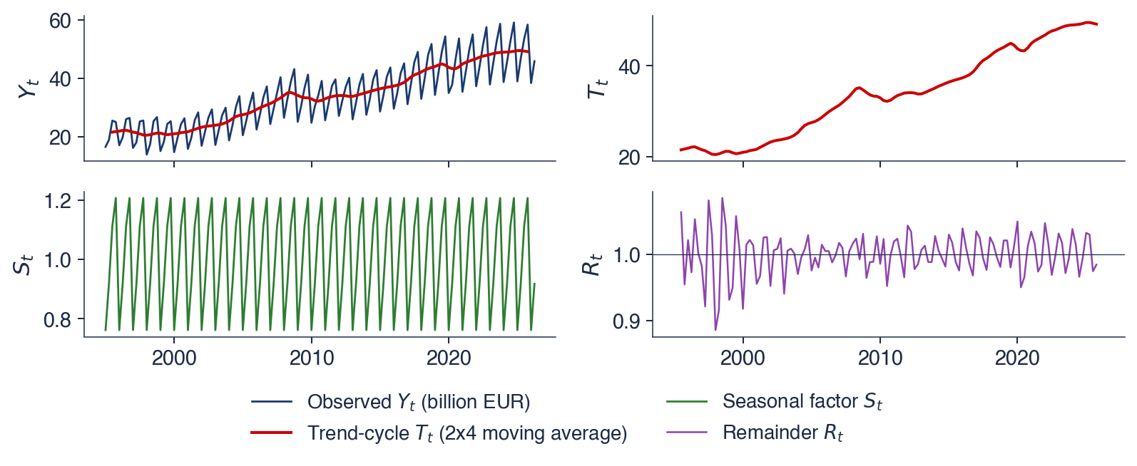
The chart applies the classical multiplicative decomposition with \(m = 4\) to Romanian real GDP. The top panel shows the observed series together with the estimated trend-cycle; the next panels show the trend-cycle alone, the seasonal factors and the remainder. The multiplicative form is chosen because the seasonal swing of GDP grows with its level.
The panels are read from top to bottom as a chain of divisions. The trend-cycle is smooth and shows the growth and the recessions of 2009 and 2020. The seasonal panel repeats the same four factors every year, as the classical method imposes. The remainder fluctuates around 1, and its larger deviations mark the quarters that neither trend nor season explains.
In brief
Classical multiplicative decomposition, \(m = 4\): observed series and trend-cycle, trend-cycle, seasonal factors, remainder
The table gives the estimated seasonal factor \(\hat S_q\) of each quarter \(q\): 0.762 for Q1, 0.918 for Q2, 1.113 for Q3 and 1.207 for Q4. In percentages relative to the trend, a typical first quarter lies 23.8% below the trend, a typical second quarter 8.2% below, a typical third quarter 11.3% above, and a typical fourth quarter 20.7% above. The four factors average to 1, as the normalisation requires. Their ratio, \(1.207 / 0.762\), shows that a fourth quarter is about 58% larger than a first quarter for purely seasonal reasons.
The remainder has a standard deviation of about 3.3%: in a typical quarter, GDP deviates by about 3% from the product of trend and season. The deviations are larger in the 1990s and in 2020, years of economic turbulence and of the pandemic. The practical consequence concerns growth rates. Comparing a quarter with the previous quarter of the raw series mixes growth with the seasonal swing; a quarter must be compared with the same quarter of the previous year, or the comparison must be made on the seasonally adjusted series.
In brief
Quarter
\(\hat S_q\)
relative to trend
Q1
0.762
\(\ensuremath{-}23.8\)%
Q2
0.918
\(\ensuremath{-}8.2\)%
Q3
1.113
\(+\)11.3%
Q4
1.207
\(+\)20.7%
Reading the factors
\(\hat S_q\): the estimated seasonal factor of quarter \(q\)
a typical first quarter is 23.8% below the trend, a typical fourth quarter 20.7% above it
Q4 is about 58% larger than Q1 for purely seasonal reasons
Remainder
standard deviation about 3.3%; larger in the 1990s and in 2020
Consequence: compare a quarter with the same quarter of the previous year, never with the previous quarter of the raw series
STL, the Seasonal and Trend decomposition using LOESS, was proposed by Cleveland et al. (1990). LOESS (locally estimated scatterplot smoothing) estimates a smooth curve by fitting, around each point, a weighted regression in which nearby observations receive larger weights. STL alternates two such smoothers: one estimates the seasonal component from the values of the same season in different years, the other estimates the trend from the series with the season removed.
STL has three advantages over the classical method. The seasonal pattern may change slowly from year to year, because each season is smoothed over the years instead of being averaged into one constant factor. The trend is estimated up to the last observation. And a robust version gives low weights to outliers, so that they go into the remainder and do not distort the season or the trend. It has two limits: it is additive only, so for multiplicative series it is applied to \(\ln y_t\), and it does not handle calendar effects such as the number of working days or the date of Easter. Statistical offices use X-13ARIMA-SEATS or TRAMO-SEATS, which build on ARIMA models and include calendar effects; they are presented in Chapter 4.
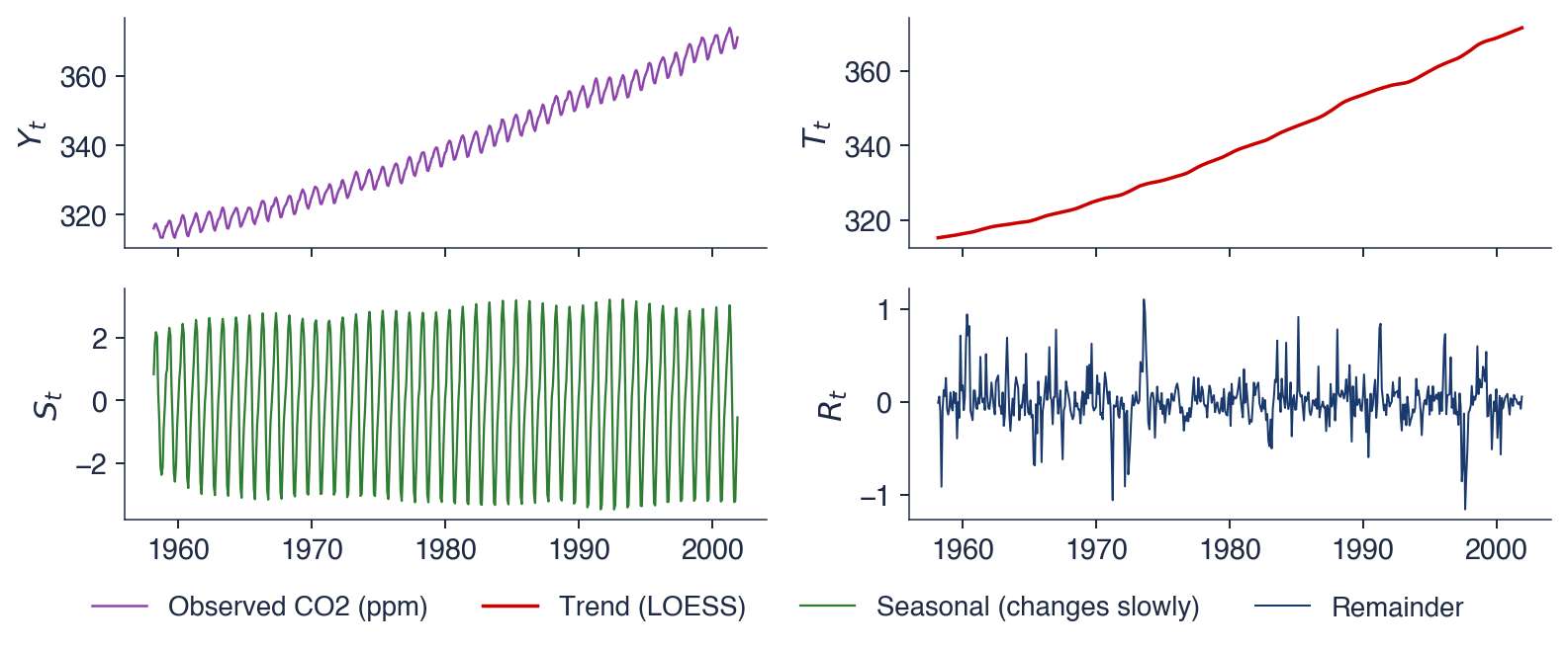
The chart applies a robust STL with period 12 to the monthly CO2 series. The four panels show, from top to bottom, the observed series, the trend, the seasonal component and the remainder, all in ppm. Because the decomposition is additive, the four panels add up: observed equals trend plus seasonal plus remainder in every month.
The scales of the panels should be compared before their shapes. The trend spans about 55 ppm, the seasonal component a few ppm, and the remainder well under one ppm. The decomposition thus says at a glance which component dominates the variation of the series.
In brief
Robust STL with period 12 on the monthly CO2 series: observed, trend, seasonal, remainder (ppm)
The trend is smooth and slightly convex: the rise accelerates over the sample, as the interpretation of the raw series suggested. The seasonal component reaches its maximum in May and its minimum in October. In winter and spring the decay of fallen leaves releases CO2 and the concentration builds up; in summer photosynthesis absorbs it, and the concentration falls until the growing season ends.
The yearly range of the seasonal component grows from 4.9 ppm in 1959 to 6.3 ppm in 2001, an increase of about 28%. The level rose by about 17% over the same period, from 316.1 to 371.0 ppm, so the growth of the wave is not proportional to the level, and neither a constant additive season nor a multiplicative one describes it exactly. STL captures it because it lets the season change.
The remainder has a standard deviation of 0.25 ppm, small compared with the season: trend and season explain almost all of the variation. The larger spikes of the remainder deserve a check against the history of the station, such as interruptions or changes of instruments, before they are treated as noise.
In brief
Trend: smooth, slightly convex: the rise accelerates
Seasonal: maximum in May, minimum in October
winter and spring: decay of fallen leaves releases CO2; summer: photosynthesis absorbs it
the yearly range grows from 4.9 ppm (1959) to 6.3 ppm (2001): STL lets the season change
Remainder: standard deviation 0.25 ppm
small compared with the season: trend and season explain almost everything
check the larger spikes against the history of the station before calling them noise
A series is described by its trend, its seasonality, which has a fixed period, its cycle, which has none, and its remainder. The decomposition is additive if the seasonal swing has a constant size and multiplicative if it grows with the level; logs turn the second into the first.
A centred \(2 \times m\) moving average removes the season and estimates the trend-cycle; averaging the detrended values by season gives the seasonal factors. For Romanian GDP, the first quarter lies about 23.8% below the trend and the fourth about 20.7% above it. STL lets the seasonal pattern change over time and is robust to outliers.
In brief
Trend, seasonality (fixed period), cycle (no fixed period), remainder
Additive if the seasonal swing is constant, multiplicative if it grows with the level; logs turn one into the other
A centred \(2 \times m\) moving average removes the season and estimates the trend-cycle
Romanian GDP: Q1 about 23.8% below the trend, Q4 about 20.7% above it
STL lets the seasonal pattern change and is robust to outliers
Section summary
The decomposition separates what repeats with a known period from what evolves slowly and from what is left. The classical method, based on moving averages, shows the logic of the separation; STL relaxes its assumption of a fixed season. For forecasting, the season is the most reliable component and the cycle the least. The next section introduces the notation of the course and the autocorrelation function, which detects the same components numerically.
Notation, transformations and the ACF
This section fixes the notation used in all chapters, introduces the transformations that turn a series with trend and changing variance into one that is easier to model, and defines the sample autocorrelation function (ACF). The ACF measures how strongly a series is related to its own past and recognises trend, seasonality and the absence of memory in its shape.
The observation at time \(t\) is \(y_t\), for \(t = 1, \ldots, T\), and the sample mean is \(\bar y = \frac{1}{T}\sum_t y_t\). The lag operator \(L\) shifts a series back one period, \(L y_t = y_{t-1}\), and its powers shift it further, \(L^k y_t = y_{t-k}\). Writing shifts as an operator turns lags into algebra: the models of Chapter 2 are polynomials in \(L\).
The first difference is \(\Delta y_t = y_t - y_{t-1}\), which in operator form is \(\Delta = 1 - L\). The seasonal difference is \(\Delta_m y_t = y_t - y_{t-m}\), with \(\Delta_m = 1 - L^m\); for quarterly data, \(\Delta_4 y_t\) compares a quarter with the same quarter of the previous year. The forecast of \(y_{T+h}\) made with the data up to \(T\) is written \(\hat y_{T+h|T}\), where \(h\) is the horizon, and the forecast error is \(e_t = y_t - \hat y_t\). Hats mark estimates and forecasts, and Greek letters such as \(\phi\),\(\theta\) and \(\alpha\) mark parameters.
In brief
Symbol
Meaning
\(y_t\), \(t = 1, \ldots, T\)
the observation at time \(t\); \(T\) observations in the sample
\(\bar y = \frac1T \sum_t y_t\)
the sample mean
\(L y_t = y_{t-1}\)
the lag operator: shifts the series back one period; \(L^k y_t = y_{t-k}\)
\(\Delta y_t = y_t - y_{t-1}\)
the first difference, \(\Delta = 1 - L\)
\(\Delta_m y_t = y_t - y_{t-m}\)
the seasonal difference, \(\Delta_m = 1 - L^m\)
\(\hat y_{T+h|T}\)
the forecast of \(y_{T+h}\) made with the data up to \(T\); \(h\) is the horizon
\(e_t = y_t - \hat y_t\)
the forecast error
Hats (\(\hat{\ }\)) mark estimates and forecasts; Greek letters (\(\phi, \theta, \alpha\)) mark parameters
The logarithm \(\ln y_t\) stabilises a variance that grows with the level: in logs, a multiplicative pattern becomes additive and swings of constant percentage become swings of constant size. The growth rate over one period is \(g_t = 100\,(y_t / y_{t-1} - 1)\). For small changes it is approximated by the difference of logs, \(100\,\Delta \ln y_t \approx g_t\), because \(\ln(1+x) \approx x\) for small \(x\). The annual growth rate of a quarterly series, \(100\,(y_t / y_{t-4} - 1)\), compares the same quarters, so the season cancels.
The worked example uses Romanian GDP: 38.7 in 2024 Q1, 59.2 in 2024 Q4 and 38.9 in 2025 Q1. Over one quarter, \(100\,(38.9 / 59.2 - 1) \approx -34\%\): a fall of a third, which is not a collapse of the economy but the effect of winter. Over one year, \(100\,(38.9 / 38.7 - 1) \approx +0.5\%\): the economy barely grew. The same observation gives two opposite impressions depending on the comparison, and only the annual rate measures growth.
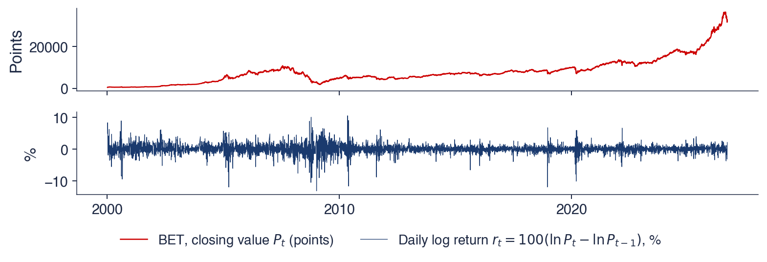
For prices, the standard transformation is the log return, \(r_t = 100\,(\ln P_t - \ln P_{t-1})\), in percent, where \(P_t\) is the price on day \(t\). Log returns add up over time: the log return over a period is the sum of the daily log returns within it.
In brief
Logarithm\(\ln y_t\): stabilises a variance that grows with the level
Growth rate over one period: \(g_t = 100\,(y_t / y_{t-1} - 1)\)
log approximation: \(100\,\Delta \ln y_t \approx g_t\) for small changes
Annual growth rate of a quarterly series: \(100\,(y_t / y_{t-4} - 1)\)
it compares the same quarters, so the season cancels out
Worked example: Romanian GDP, 2024 Q1 = 38.7, 2024 Q4 = 59.2, 2025 Q1 = 38.9
over one quarter: \(100\,(38.9 / 59.2 - 1) \approx -34\%\): not a collapse, only winter
over one year: \(100\,(38.9 / 38.7 - 1) \approx +0.5\%\): the economy barely grew
Log return of a price: \(r_t = 100\,(\ln P_t - \ln P_{t-1})\), in %; \(P_t\): the price on day \(t\)
The top panel shows the closing value of the BET index since 2000; the bottom panel shows its daily log returns in percent, over 6,670 trading days. The two panels are the same data before and after the transformation \(r_t = 100\,\Delta \ln P_t\).
The top panel has a trend, long rises and a deep fall in 2008. The bottom panel has none of these: the returns fluctuate around zero, and what changes over time is the width of the band in which they move. The transformation has moved the interesting feature of the series from the level to the variance.
In brief
Top: closing value of the BET since 2000; bottom: daily log returns in % (6 670 trading days)
The price has a trend; the returns do not. The daily returns fluctuate around a mean of 0.064% with a standard deviation of 1.40%, which corresponds to about 22% a year, since daily volatility is annualised by the factor \(\sqrt{252} \approx 15.9\). The additivity of log returns links the mean to the growth seen in the section on real data: 6,670 days times 0.064% gives about 4.26, and \(e^{4.26} \approx 71\), the multiple by which an investment in the BET grew.
The extreme days are far from the mean: the worst was −13.1% on 7 January 2009, the best +10.6% on 10 May 2010, both more than seven standard deviations away. Calm and turbulent periods alternate: large moves cluster in 2008–2010 and in March 2020. This volatility clustering, the subject of Chapter 5, means that the size of today's move says something about the size of tomorrow's.
Differencing the log price removes the trend. Most models of the course work on transformed series of this kind, whose mean does not drift, and then translate their forecasts back to the original scale.
In brief
The price has a trend; the returns do not
returns fluctuate around a mean of 0.064% a day, with a standard deviation of 1.40% (about 22% a year)
Extreme days
worst: \(-\)13.1% on 7 January 2009; best: +10.6% on 10 May 2010
Calm and turbulent periods alternate
large moves cluster in 2008–2010 and in March 2020: volatility clustering (Chapter 5)
Differencing the log price removes the trend: most models of the course work on such transformed series
where \(k\) is the lag in periods and \(\bar y\) the sample mean. Each product is positive when \(y_t\) and \(y_{t-k}\) lie on the same side of the mean and negative otherwise, so \(c_k\) is positive when values \(k\) periods apart tend to be both high or both low. The divisor is \(T\) and not \(T - k\); this choice keeps the estimated autocovariances consistent with a valid covariance structure.
The sample autocorrelation is
\[r_k = \frac{c_k}{c_0},\]
(0.6)
where \(c_0\) is the sample variance, the autocovariance at lag 0; \(r_k\) lies between \(-1\) and \(1\). The autocorrelation function (ACF) is the sequence \(r_1, r_2, \ldots\), plotted against \(k\) in a chart called the correlogram.
The correlogram is read against the reference band \(\pm 1.96/\sqrt{T}\), where 1.96 is the 97.5% quantile of the standard Normal distribution. If the series were independent noise, each \(r_k\) would be approximately Normal with mean 0 and standard deviation \(1/\sqrt{T}\), and about 95% of the \(r_k\) would fall inside the band. A value outside the band is a sign of dependence at that lag; among many lags, about one in twenty falls outside by chance. The theory behind the band, with stationarity, white noise and the Ljung–Box test, comes in Chapter 1.
In brief
Question: how strongly is \(y_t\) related to its own value \(k\) periods earlier?
The series has \(T = 6\) values: 2, 4, 3, 5, 4, 6. Their sum is 24, so \(\bar y = 4\), and the deviations from the mean are \(-2, 0, -1, 1, 0, 2\). The sum of squared deviations is \(4 + 0 + 1 + 1 + 0 + 4 = 10\), so \(c_0 = 10/6\). The products of consecutive deviations, \((y_t - \bar y)(y_{t-1} - \bar y)\) for \(t = 2, \ldots, 6\), are \(0, 0, -1, 0, 0\), with sum \(-1\), so \(c_1 = -1/6\) and
\[r_1 = \frac{-1/6}{10/6} = -0.1.\]
At lag 2 the products pair values two periods apart: \((-1)(-2) + (1)(0) + (0)(-1) + (2)(1) = 4\), so \(r_2 = 4/10 = 0.4\). The divisor \(T\) cancels in the ratio, so \(r_k\) is simply the sum of lagged products divided by the sum of squares.
With six observations the band is \(\pm 1.96/\sqrt{6} = \pm 0.80\). Both values lie well inside it, so neither is distinguishable from 0 by this criterion. The example shows why short series give little evidence about dependence: an autocorrelation of 0.4 is large, but with six observations it is within the range that independent noise produces.
In brief
\(t\)
\(y_t\)
\(y_t - \bar y\)
\((y_t - \bar y)(y_{t-1} - \bar y)\)
1
2
\(-2\)
–
2
4
\(0\)
\(0\)
3
3
\(-1\)
\(0\)
4
5
\(1\)
\(-1\)
5
4
\(0\)
\(0\)
6
6
\(2\)
\(0\)
sum
24
0
\(-1\)
\(T = 6\), \(\bar y = 24 / 6 = 4\)
sum of squared deviations: \(4 + 0 + 1 + 1 + 0 + 4 = 10\)
\(r_1 = \dfrac{-1/6}{10/6} = -0.1\)
at lag 2: products \((-1)(-2) + (1)(0) + (0)(-1) + (2)(1) = 4\), so \(r_2 = 0.4\)
Interpretation
band \(\pm 1.96/\sqrt 6 = \pm 0.80\): with 6 observations, neither value is distinguishable from 0
The chart shows the sample ACF for lags 1 to 36 of three series, with the band \(\pm 1.96/\sqrt{T}\) shaded. The left panel is the level of CO2, the centre panel the monthly electricity generation, the right panel the daily log returns of the BET. Each bar is one \(r_k\); the horizontal axis is the lag \(k\), in months for the first two series and in trading days for the third.
The three panels were chosen because they show the three typical shapes of a correlogram: a slow decline, a wave with peaks at multiples of the seasonal period, and bars that are almost all close to zero. The band is narrow for the BET, because \(T\) is large, and wider for the monthly series.
In brief
Sample ACF for lags 1–36; shaded: the band \(\pm 1.96/\sqrt{T}\). Left: CO2 level; centre: monthly electricity generation; right: BET daily log returns
The CO2 level has \(r_1 = 0.993\) and still 0.80 at lag 36. A slow, almost linear decay is the signature of a trend: values far apart in time are all on the same side of the mean, below it at the start of the sample and above it at the end, so the level remembers its past for years. The ACF of a trending level is dominated by the trend and says little about the short-run dynamics.
Electricity generation has \(r_1 = 0.75\),\(r_6 = 0.13\) and \(r_{12} = 0.59\), with peaks at 12, 24 and 36 months: this January resembles last January. The band for this series is about \(\pm 0.13\), so the seasonal peaks are clearly significant. Peaks at multiples of the period \(m\) are the signature of seasonality.
The BET returns have almost no memory: \(r_1 = 0.109\),\(r_2 = 0.022\), against a band of \(\pm 0.024\). The first autocorrelation is small but significant, and 8 of the 36 lags fall outside the band, more than the one or two that independent noise would produce. Such autocorrelations are hard to exploit after trading costs. The absolute returns have \(r_1 = 0.40\): the size of the moves is predictable, their sign much less, which is volatility clustering again (Chapter 5). The general rule is to transform first and then look at the ACF.
In brief
Trend: CO2, \(r_1 = \) 0.993, still 0.80 at lag 36
a slow, almost linear decay is the signature of a trend: the level remembers its past for years
The lag operator gives \(L y_t = y_{t-1}\), the first difference is \(\Delta = 1 - L\) and the seasonal difference \(\Delta_m = 1 - L^m\);\(\hat y_{T+h|T}\) is the forecast for horizon \(h\) made at time \(T\). Logs stabilise the variance, differences remove the trend, and annual rates remove the season.
The sample autocorrelation \(r_k = c_k / c_0\) is compared with the band \(\pm 1.96/\sqrt T\). Its shape identifies the dominant component: a slow decay indicates a trend, peaks at \(m, 2m, \ldots\) indicate seasonality, and values all close to zero indicate little linear memory.
In brief
\(L y_t = y_{t-1}\), \(\Delta = 1 - L\), \(\Delta_m = 1 - L^m\); \(\hat y_{T+h|T}\) is the forecast for horizon \(h\)
Logs stabilise the variance; differences remove the trend; annual rates remove the season
\(r_k = c_k / c_0\), compared with the band \(\pm 1.96/\sqrt T\)
Slow decay: trend; peaks at \(m, 2m, \ldots\): seasonality; all close to 0: little linear memory
Section summary
Transformations and the ACF are the first diagnostic tools of every analysis in the course. A series with a trend or a changing variance is transformed before it is modelled, and the correlogram of the transformed series shows which dependence remains. The next section uses the dependence on the recent past to build the first forecasting methods.
Exponential smoothing
Exponential smoothing forecasts a series with weighted averages of its past values, in which the weights decline geometrically with age. The methods were developed in industry in the 1950s to forecast sales and inventories, and they remain among the most accurate simple forecasting methods. This section derives simple exponential smoothing (SES), shows the role of the smoothing constant on the EUR/RON series, and extends the method to trend and seasonality with Holt and Holt–Winters.
where \(\ell_t\) is the smoothed level at time \(t\) and \(\alpha\) the smoothing constant. Rewritten as \(\ell_t = \ell_{t-1} + \alpha\,(y_t - \ell_{t-1})\), the equation says that the level moves from \(\ell_{t-1}\) towards the new observation by the fraction \(\alpha\) of the last forecast error. The forecast for every horizon is the last level, \(\hat y_{T+h|T} = \ell_T\), a flat line.
The name comes from substituting the equation into itself repeatedly:
The weights fall geometrically, as an exponential function of the age of the observation; with \(\alpha = 0.5\) they are 0.5, 0.25, 0.125 and so on, and they sum to 1.
A small \(\alpha\) spreads the weight over many past values: the method has a long memory, its forecasts are smooth, and it reacts slowly to changes. A large \(\alpha\) concentrates the weight on the latest values. With \(\alpha = 1\) the level equals the last observation and SES becomes the naive forecast, \(\hat y_{T+1} = y_T\). In practice \(\alpha\) is estimated by minimising the sum of squared one-step forecast errors over the sample.
In brief
Idea: forecast with a weighted average of the past, recent values weighing more
\(\ell_t\): the smoothed level at time \(t\); \(\alpha\): the smoothing constant; \(\ell_t\) moves from \(\ell_{t-1}\) towards \(y_t\) by the fraction \(\alpha\)
forecast for every horizon: \(\hat y_{T+h|T} = \ell_T\), a flat line
The table applies (0.7) with \(\alpha = 0.5\) to four observations, 10, 12, 11 and 13. The initial level is the first observation, \(\ell_0 = 10\). At \(t = 1\) the forecast is \(\ell_0 = 10\) and the observation is 10, so the level stays at 10. At \(t = 2\) the observation is 12 and the new level is \(0.5 \times 12 + 0.5 \times 10 = 11\). At \(t = 3\) the forecast 11 equals the observation, so the level stays at 11. At \(t = 4\) the level becomes \(0.5 \times 13 + 0.5 \times 11 = 12\).
The forecast for \(t = 5\) and for every later period is 12: SES does not extrapolate trends, it only tracks the level. The one-step errors are 0, 2, 0 and 2, all non-negative: the forecasts lag behind the rising data. Errors that keep the same sign are a symptom of a trend that the method does not model, and the reason for Holt's extension later in this section.
In brief
\(t\)
\(y_t\)
\(\hat y_{t|t-1} = \ell_{t-1}\)
\(\ell_t = 0.5\,y_t + 0.5\,\ell_{t-1}\)
0
–
–
\(\ell_0 = 10\)
1
10
10
10
2
12
10
11
3
11
11
11
4
13
11
12
5
?
12
–
initial level \(\ell_0 = 10\) (the first observation)
\(t = 2\): \(0.5 \times 12 + 0.5 \times 10 = 11\)
\(t = 4\): \(0.5 \times 13 + 0.5 \times 11 = 12\)
Interpretation
the forecast for \(t = 5\) and every later period is 12: SES does not extrapolate trends
one-step errors: 0, 2, 0, 2: the forecasts lag behind the rising data
The dots in the chart are the monthly averages of the BNR reference rate from January 2015 to September 2026. The two lines are one-step SES forecasts \(\hat y_{t|t-1}\), each computed with the data available at the end of the previous month, for two values of the smoothing constant: \(\alpha = 0.1\) and \(\alpha = 0.7\).
The chart is read by comparing each line with the dots. A good one-step forecast stays close to the next dot. A forecast that stays systematically below the dots during a rise, or that needs many months to reach a new level after a jump, has too much memory for this series.
In brief
Dots: monthly averages of the BNR reference rate, January 2015 – September 2026; lines: one-step SES forecasts \(\hat y_{t|t-1}\) with \(\alpha = 0.1\) and \(\alpha = 0.7\)
With \(\alpha = 0.1\) the forecast is smooth but always below the rising rate. The average age of the observations it weighs is \((1-\alpha)/\alpha = 9\) months, so it remembers several years of data, and after the jump of 2025 it needs many months to catch up. With \(\alpha = 0.7\) the average age is under half a month: the forecast follows the data closely, one month late.
The estimated smoothing constant is \(\hat\alpha = 1.00\). The best SES forecast of next month is therefore this month's average, and SES reduces to the naive forecast. This is typical of exchange rates and prices: the last value contains almost all the information about the next one, as in a random walk (Chapter 1), and averaging older values only adds outdated information. An estimated \(\alpha\) near 1 is a finding about the series, not a failure of the method.
In brief
\(\alpha = 0.1\): smooth, but always below the rising rate
it remembers several years: after the jump of 2025 it needs many months to catch up
\(\alpha = 0.7\): follows the data closely, one month late
Estimated\(\hat\alpha = \) 1.00
the best SES forecast of next month is this month's average: SES reduces to the naive forecast
typical of exchange rates and prices: the last value contains almost all the information (a random walk, Chapter 1)
An estimated \(\alpha\) near 1 is a finding about the series, not a failure of the method
The level is updated towards \(y_t\) starting from the previous level plus the previous slope, which is where the series was expected to be. The slope \(b_t\) is the estimated change of the level per period; it is updated towards the latest change of the level, \(\ell_t - \ell_{t-1}\). The constant \(\beta \in (0, 1]\) smooths the slope: a small \(\beta\) gives a slope that changes slowly.
The forecast is \(\hat y_{T+h|T} = \ell_T + h\, b_T\), the last level plus \(h\) times the last slope, a straight line. Straight lines extrapolated over long horizons tend to overshoot, because trends rarely persist unchanged. The damped trend multiplies the slope by \(\phi^j\) at step \(j\), with \(0 < \phi < 1\), so that the forecast becomes \(\ell_T + (\phi + \phi^2 + \cdots + \phi^h)\, b_T\) and flattens as \(h\) grows.
In brief
Holt (1957): level plus a trend\(b_t\) (Holt (1957))
where \(s_{T+h-m}\) is the latest seasonal factor of the same season; a factor \(s = 1.1\) places the season 10% above the trend line. Each component has its own smoothing constant: \(\alpha\) for the level, \(\beta\) for the slope and \(\gamma\) for the season. The multiplicative form suits series such as GDP, whose seasonal swing grows with the level; an additive form adds \(s_{T+h-m}\) instead.
Hyndman, Koehler, Snyder & Grose (2002) turned these methods into statistical models, the ETS (Error, Trend, Seasonal) family. Each component is labelled N (none), A (additive), M (multiplicative) or A\(_d\) (additive damped); ETS(M,A\(_d\),M), for example, has multiplicative errors, a damped trend and a multiplicative season. Because each method becomes a model with a likelihood, it gives forecast intervals and an information criterion for choosing among methods (Chapter 2). Gardner (1985) reviews the first 25 years of exponential smoothing.
In brief
Holt–Winters (1960): adds seasonal factors \(s_t\) with period \(m\) (Winters (1960))
each method is a statistical model: N (none), A (additive), M (multiplicative), A\(_d\) (damped)
e.g. ETS(M,A\(_d\),M): multiplicative errors, damped trend, multiplicative season; it gives forecast intervals and an information criterion (Chapter 2)
A review of 25 years of exponential smoothing: Gardner (1985)
SES updates the level by \(\ell_t = \alpha y_t + (1-\alpha)\ell_{t-1}\). Its weights on past observations decline geometrically, and its forecasts are flat. A small \(\alpha\) gives smooth forecasts that react slowly; \(\alpha = 1\) gives the naive forecast.
On the monthly EUR/RON, the estimated \(\hat\alpha\) is 1.00, so the last value is the best SES forecast. Holt adds a trend and Holt–Winters a season, and the ETS framework turns these methods into statistical models with forecast intervals.
Small \(\alpha\): smooth and slow; \(\alpha = 1\): the naive forecast
EUR/RON: \(\hat\alpha = \) 1.00, the last value is the best SES forecast
Holt adds a trend, Holt–Winters a season; ETS turns them into statistical models
Section summary
Exponential smoothing forecasts with geometrically weighted averages of the past, extended with a slope and seasonal factors when the series has a trend and a season. The estimated smoothing constant is itself informative: close to 1 for exchange rates, smaller for series in which the level must be separated from noise. The next section shows how to decide whether such forecasts are good.
Forecasts and their evaluation
A forecast is useful only if it is better than an obvious alternative. This section defines the forecasting setting, introduces four benchmark methods, explains why the data must be split by time into a training set and a test set, and defines the error measures. It then compares methods on Romanian electricity generation, reviews the M4 forecasting competition and runs a small competition on four Romanian and climate series.
A forecast \(\hat y_{T+h|T}\) is a statement about the value \(y_{T+h}\), made at time \(T\). It may use only the information available at \(T\), called the information set; a forecast that uses later data, even indirectly, is not a forecast. The horizon \(h = 1, 2, \ldots\) counts the periods ahead, and the uncertainty grows with \(h\), because more unforeseen shocks accumulate between \(T\) and \(T+h\).
A point forecast is one number. An interval forecast is a range that contains \(y_{T+h}\) with a stated probability, for example 95%, and it conveys how much the point forecast can be trusted. Two conditions make a series forecastable. The first is a stable pattern, as in the CO2 series, rather than movements driven by news, as in exchange rates. The second is that the forecast does not change the outcome: a weather forecast does not change the weather, but a price forecast published to millions of traders changes the price, because they trade on it.
In brief
Forecast\(\hat y_{T+h|T}\): a statement about \(y_{T+h}\) made at time \(T\)
it may use only the information available at \(T\): the information set
\(h = 1, 2, \ldots\): the horizon; uncertainty grows with \(h\)
Point and interval forecasts
point: one number; interval: a range that contains \(y_{T+h}\) with a stated probability (e.g. 95%)
What makes a series forecastable
a stable pattern (CO2) rather than one driven by news (exchange rates)
a forecast that does not change the outcome: a price forecast published to millions of traders changes the price
The mean method forecasts every future value by the sample mean, \(\hat y_{T+h|T} = \bar y\): the future looks like the average past. The naive method uses the last value, \(\hat y_{T+h|T} = y_T\); it is optimal for a random walk, the usual model of exchange rates and prices. The seasonal naive method repeats the value of the same season one period earlier, \(\hat y_{T+h|T} = y_{T+h-m}\) for \(h \le m\): next January equals last January. It is a strong benchmark for highly seasonal series.
The drift method adds to the last value the average past change per period,
which amounts to extending the straight line between the first and the last observation. Each of the four methods corresponds to a simple model of the series: no dynamics, a random walk, a fixed season, a random walk with drift. A new model is worth using only if it beats these benchmarks on data it has not seen.
In brief
Mean: \(\hat y_{T+h|T} = \bar y\)
the future looks like the average past
Naive: \(\hat y_{T+h|T} = y_T\)
the last value; optimal for a random walk (exchange rates, prices)
The diagram shows how a series is split for evaluation. The data are split by time, never at random. The training set contains the first observations and is used to choose and estimate the method; the test set contains the last \(h\) observations, which are kept hidden and used only to measure the errors. A random split, as in cross-sectional machine learning, would place future observations in the training set; the model would then see the future, and its errors would look too small.
A single split gives one sample of forecast errors, which can be unrepresentative. The rolling origin, also called time series cross-validation, repeats the exercise with the forecast origin moved forward: each row of the diagram trains on a longer history and tests on the following periods. Averaging the errors over origins gives a more stable estimate of accuracy.
penalises large errors more, because they are squared; it is always at least as large as the MAE, and the gap between the two grows when a few errors are much larger than the rest.
The mean absolute percentage error, \(\text{MAPE} = \frac{100}{h} \sum_j |e_{T+j} / y_{T+j}|\), has no units, so it can compare series measured in different units, but it is useless when \(y\) is close to 0, as for inflation rates or returns, because the division explodes. The mean absolute scaled error of Hyndman & Koehler (2006) divides the MAE on the test set by the in-sample MAE of the naive method. For seasonal series, such as those of this chapter, the scale is the in-sample MAE of the seasonal naive method, with period \(m\), as in the M4 competition:
With \(m = 1\) the formula gives the original, non-seasonal scale. A MASE below 1 means that the method's errors are smaller than those the seasonal naive method made on the training data. Because it has no units and does not divide by \(y\), the MASE is comparable across series.
In brief
Errors on the test set: \(e_{T+j} = y_{T+j} - \hat y_{T+j|T}\), \(j = 1, \ldots, h\)
MAE (mean absolute error) \(= \frac1h \sum_j |e_{T+j}|\)
in the units of the series; easy to explain
RMSE (root mean squared error) \(= \sqrt{\frac1h \sum_j e_{T+j}^2}\)
without units, but useless when \(y\) is close to 0 (inflation, returns)
MASE (mean absolute scaled error) \(=\) MAE \(/\) in-sample MAE of the naive method (Hyndman & Koehler (2006)); for seasonal series, of the seasonal naive method (as in M4)
below 1: better than that benchmark on the training data; comparable across series
The table has two years of quarterly training data (10, 14, 18, 12 and 11, 15, 20, 13) and a third year as test set (12, 16, 21, 14). The naive forecast repeats the last training value, 13, for all four quarters; its errors are \(-1, 3, 8, 1\). The MAE is \((1 + 3 + 8 + 1)/4 = 3.25\) and the RMSE is \(\sqrt{(1 + 9 + 64 + 1)/4} = \sqrt{18.75} = 4.33\).
The seasonal naive forecast repeats the quarters of year 2: 11, 15, 20, 13. Its errors are all equal to 1, so MAE = RMSE = 1. The naive forecast misses the season: its large error in the third quarter, 8, contributes 64 of the 75 units of the sum of squares and dominates the RMSE. On seasonal data the seasonal naive method is the benchmark to beat.
The chart applies four methods to Romanian electricity generation. The test set covers August 2024 to July 2026, 24 months; the training data are all earlier months, from January 2008. The dashed lines are forecasts made once, at the end of the training set, for all 24 months of the test set, so the horizon goes from 1 to 24 months.
The methods are the naive forecast, the seasonal naive forecast, SES and Holt–Winters. The chart is read by comparing each dashed line with the observed series in the test period: a flat line cannot follow the winter peaks, a copy of the last year follows the season but not the change in level.
In brief
Test set: August 2024 – July 2026 (24 months); training data: all earlier months; dashed: forecasts made once, at the end of the training set
The table gives the four error measures on the test set; MAE and RMSE are in TWh per month. The naive method has MAE 0.28, RMSE 0.33, MAPE 7.3% and MASE 0.82. The seasonal naive method has MAE 0.28, RMSE 0.38, MAPE 7.2% and MASE 0.83. SES has MAE 0.28, RMSE 0.32, MAPE 7.1% and MASE 0.81. Holt–Winters has MAE 0.17, RMSE 0.21, MAPE 4.5% and MASE 0.51.
Holt–Winters has the smallest error on every measure, because it combines a falling level with the winter peak; its MAE is about 40% lower than that of the other three. The seasonal naive method is not better than the naive one here: it copies the high winter of 2023–2024 into a lower 2024–2026, and its RMSE, 0.38, is the largest of the four, a sign of a few large errors in the winter months.
A test period of 24 months is one sample of forecast errors, from one origin. A rolling origin, with many test periods, gives a firmer answer about which method is more accurate on this series.
In brief
Method
MAE
RMSE
MAPE
MASE
Naive
0.28
0.33
7.3%
0.82
Seasonal naive
0.28
0.38
7.2%
0.83
SES
0.28
0.32
7.1%
0.81
Holt–Winters
0.17
0.21
4.5%
0.51
MAE and RMSE in TWh per month
Holt–Winters has the smallest error on every measure
it combines a falling level with the winter peak
The seasonal naive method is not better than the naive one here
it copies the high winter of 2023–2024 into a lower 2024–2026
One test period of 24 months is one sample: a rolling origin gives a firmer answer
The question behind the M competitions is which forecasting methods work best on real data. The competitions were started by Spyros Makridakis in 1982. Their design removes the main risk of method comparisons: forecasts are submitted blind, without access to the test data, and scored on hidden test data by the organisers.
The M4 competition, held in 2018, used 100,000 series, from yearly to hourly, and compared 61 methods (Makridakis, Spiliotis & Assimakopoulos, 2020). Twelve of the 17 most accurate methods were combinations of several methods. The winner was a hybrid of exponential smoothing and a neural network. Pure machine learning methods did poorly: none of them beat a simple combination of exponential smoothing methods.
For this course the lessons are methodological. Benchmarks come first, accuracy is measured out of sample, and conclusions require many series rather than one. The same lesson had appeared in M3 (Makridakis & Hibon, 2000): a more complex method is not automatically more accurate.
In brief
The question: which forecasting methods work best on real data?
the M competitions, started by Spyros Makridakis in 1982: forecasts submitted blind, scored on hidden test data
The chart reproduces the logic of the M competitions on a small scale: four methods, the naive, seasonal naive, SES and Holt–Winters forecasts, on four seasonal series, GDP, the HICP, electricity generation and CO2. The test sets are the last 8 quarters for GDP and the last 24 months for the monthly series.
Each bar is the MASE of one method on one series, on a logarithmic scale; the dashed line marks MASE = 1. Because the MASE is scaled by the in-sample error of the seasonal naive method, the bars of different series can be compared directly. A bar below the line means that the method forecast the test set better than the seasonal naive method forecast the training data.
In brief
MASE on the test set (log scale) of four methods on four seasonal series; test sets: the last 8 quarters (GDP) or 24 months; dashed line: MASE = 1
Holt–Winters wins on three of the four series. On CO2 its MASE is 0.26, against 1.45 for the seasonal naive method; on the HICP it is 0.68, against 2.24 for the naive method. On electricity its MASE is 0.51, as in the previous comparison.
On GDP the seasonal naive method wins, with a MASE of 0.29 against 0.65 for Holt–Winters. Growth stalled in 2025–2026, as the annual growth rate of 0.5% in 2025 Q1 showed; the trend learnt by Holt–Winters from the earlier years overshoots, while the seasonal naive method, which assumes no growth, happens to be closer. The naive method and SES fail on the seasonal series: on GDP their MASE is 4.62 and 4.39, because they ignore the season and forecast a flat line through the quarterly swing.
As in M4, no method wins everywhere, and a simple benchmark can beat a better-looking model. The ranking also depends on the test period: with a different stretch of GDP data, the trend of Holt–Winters could have been an advantage.
In brief
Holt–Winters wins on 3 of 4 series
CO2: MASE 0.26 against 1.45 for the seasonal naive method; HICP: 0.68 against 2.24 for the naive one
GDP: the seasonal naive method wins, MASE 0.29 against 0.65
growth stalled in 2025–2026: the trend learnt by Holt–Winters overshoots
Naive and SES fail on seasonal series
GDP: MASE 4.62 (naive) and 4.39 (SES): they ignore the season
As in M4: no method wins everywhere, and a simple benchmark can beat a better-looking model
A forecast \(\hat y_{T+h|T}\) uses only the information up to \(T\), and its uncertainty grows with the horizon \(h\). The benchmarks are the mean, naive, seasonal naive and drift methods; a new method must beat them out of sample.
The data are split by time, and MAE, RMSE, MAPE and MASE are measured on the test set only. The M4 competition and the mini-competition on Romanian data agree: simple methods are strong, combinations and Holt–Winters do well, and no method wins everywhere.
In brief
\(\hat y_{T+h|T}\) uses only the information up to \(T\); uncertainty grows with \(h\)
Benchmarks: mean, naive, seasonal naive, drift
Split by time; measure MAE, RMSE, MAPE and MASE on the test set only
M4 and our mini-competition: simple methods are strong; combinations and Holt–Winters do well
Section summary
Forecast evaluation rests on three rules: split by time, compare with simple benchmarks, and measure errors only on data the method has not seen. The MASE makes errors comparable across series. On the series of this chapter Holt–Winters is usually the most accurate, but on Romanian GDP the seasonal naive forecast wins, a reminder that a ranking from one test period is evidence, not proof.
Tools
The computations of the course are done in Python. This section lists the libraries used throughout and reads a first script line by line: it downloads Romanian GDP, decomposes it, computes annual growth rates and forecasts it with Holt–Winters.
Five libraries cover the course. NumPy provides arrays and linear algebra (Harris et al., 2020). pandas provides tables indexed by date, with operations for changing the frequency, lagging and differencing (McKinney, 2010). matplotlib draws the charts. statsmodels implements decomposition, exponential smoothing, ARIMA and VAR models and unit-root tests (Seabold & Perktold, 2010). The arch library estimates the GARCH models of Chapter 5.
Google Colab runs notebooks in the browser, with nothing to install. A course notebook opens with one click; the menu File → Save a copy in Drive keeps a personal copy with the student's changes. Every chart of the slides has a Quantlet whose code runs in Colab, so each result of the chapter can be reproduced and modified.
The script reads Romanian real GDP directly from the Eurostat API (application programming interface), which needs no key. The URL selects the quarterly series of chain-linked volumes at 2010 prices, unadjusted, for Romania; the values arrive in million EUR and are divided by 1,000 to obtain billion EUR. The quarters become a PeriodIndex, a time index whose elements are periods rather than dates, and are then converted to timestamps.
The rest of the script repeats the main steps of the chapter in four lines. seasonal_decompose with model='multiplicative' and period=4 performs the classical multiplicative decomposition of the section on components, and the first four values of the seasonal component are the seasonal factors of the four quarters. y.shift(4) gives the value of the same quarter a year earlier, so 100 * (y / y.shift(4) - 1) is the annual growth rate in percent. ExponentialSmoothing with an additive trend and a multiplicative season of period 4 is the Holt–Winters method of (0.9), and forecast(4) returns the forecasts for the next four quarters.
In brief
import pandas as pd
from statsmodels.tsa.seasonal import seasonal_decompose
from statsmodels.tsa.holtwinters import ExponentialSmoothing

# Romanian real GDP, quarterly (Eurostat)
url = ('https://ec.europa.eu/eurostat/api/dissemination/'
       'sdmx/2.1/data/namq_10_gdp/Q.CLV10_MEUR.NSA.B1GQ.RO'
       '?format=SDMX-CSV')
t = pd.read_csv(url)
y = pd.Series(t['OBS_VALUE'].values / 1000,
              index=pd.PeriodIndex(t['TIME_PERIOD'], freq='Q'))
y = y.to_timestamp()

dec = seasonal_decompose(y, model='multiplicative', period=4)
print(dec.seasonal.iloc[:4])            # seasonal factors
yoy = 100 * (y / y.shift(4) - 1)         # annual growth, %
hw = ExponentialSmoothing(y, trend='add', seasonal='mul',
                          seasonal_periods=4).fit()
print(hw.forecast(4))                    # next four quarters
Line by line
read the series directly from the Eurostat API (no key)
PeriodIndex: quarters as the time index
classical multiplicative decomposition with \(m = 4\)
shift(4): the value of the same quarter a year earlier
Holt–Winters with additive trend and multiplicative season
API: application programming interface
Section summary
pandas, statsmodels and the other libraries of the course turn each method of this chapter into one or two lines of code. Short code also makes errors easy to hide, for example a shift by one quarter instead of four, which is why every result must be read against the chart and the definitions.
Possible contribution of AI
AI assistants write time-series code quickly and often correctly, but some errors are specific to time series and are easy to miss because the code runs. This section lists where an assistant helps, the errors to look for, and the checks that make a result trustworthy.
An AI assistant helps in three places. It can write a first draft of the code that reads a series from Eurostat or the BNR and plots it, the part of the work that requires knowledge of interfaces rather than of statistics. It can explain an error message or the arguments of a statsmodels function. And it can list candidate explanations of a pattern, such as a drop in GDP or a jump in EUR/RON, which the analyst then checks against the data and the historical record.
Some errors recur in AI-generated time-series code. A random split into training and test sets lets the model see the future, so the measured errors are too small. Growth over one quarter is called "annual growth", or shift(1) is used where shift(4) is needed, which on unadjusted GDP turns the seasonal fall of the first quarter into an apparent recession. An RMSE is computed without the square root, and a MAPE is computed on a series that crosses zero. Exercise C2 of Seminar 0 asks students to find three such errors in an AI answer.
In brief
Where an AI assistant helps
a first draft of the code that reads a Eurostat or BNR series and plots it
explaining an error message or a statsmodels function
listing candidate explanations of a pattern (a drop in GDP, a jump in EUR/RON)
Time-series errors that AI code makes often
a random train/test split, which lets the model see the future
growth over one quarter called “annual growth”; shift(1) instead of shift(4)
an RMSE without the square root; a MAPE on a series that crosses zero
Seminar 0, exercise C2: find three such errors in an AI answer
The checks start with the data. The series is plotted before any computation, and its frequency, its units and its first and last dates are compared with the source. The analyst must also know whether the series is seasonally adjusted: a model for the season needs the unadjusted series, since in the adjusted one the season has already been removed.
The evaluation is checked next. The test set must come after the training set and must be used once, at the end; a test set consulted repeatedly while choosing the method becomes part of the training data. Before any success is claimed, the method is compared with the naive and seasonal naive forecasts. Finally, the claims are checked as in the AI policy: every reference through its DOI, every number by recomputing it, and every use of AI recorded in the declaration file.
In brief
The data
plot the series first; check the frequency, the units, the first and the last date
adjusted or unadjusted? A model for the season needs the unadjusted series
The evaluation
the test set comes after the training set; it is used once, at the end
compare with the naive and seasonal naive forecasts before claiming success
The claims: the checks of the AI policy (references, numbers, AI_USE.md)
Section summary
AI assistants speed up the routine parts of the work, but the errors that matter in time series, such as leaks from the future, wrong lags and inappropriate error measures, produce code that runs and results that look plausible. The checks of this section, together with the comparison with simple benchmarks, are what makes a result trustworthy.
Conclusions
The chapter introduced the object of the course, the patterns it contains, and the first methods for describing and forecasting it. This section collects the main ideas, gives questions for self-assessment and a project idea, and links the chapter to the next one.
A time series is ordered in time, and its dependence on the past is what makes forecasting possible. It is described by four components: a trend, a seasonality with a fixed period, a cycle without a fixed period, and a remainder; the components combine additively when the seasonal swing has a constant size and multiplicatively when it grows with the level. Yule and Slutsky found the two mechanisms that generate waves in data, dependence on past values and sums of past shocks, the roots of AR and MA models.
The ACF reveals a trend by a slow decay, a season by peaks at multiples of \(m\), and the absence of memory by values close to zero. Exponential smoothing gives more weight to the recent past, with a slope and seasonal factors when needed. Every forecast must be evaluated against naive benchmarks on a test set that follows the training set in time.
In brief
A time series is ordered in time; its dependence on the past is what makes forecasting possible
Components: trend, seasonality (fixed period), cycle (no fixed period), remainder; additive or multiplicative
Yule and Slutsky: dependence and sums of shocks, the roots of AR and MA models
The ACF reveals trend (slow decay), season (peaks at \(m\)) and memory
Exponential smoothing weighs the recent past more; evaluate every forecast against naive benchmarks on a test set
The four self-assessment questions test the central ideas of the chapter. The first, on the quarter-on-quarter growth of unadjusted GDP, is answered by the worked example of the notation section. The second, on the meaning of a seasonal factor of 0.76 for the first quarter, is answered by the GDP decomposition. The third, on what an estimated \(\alpha\) close to 1 says about a series, is answered by the EUR/RON example. The fourth, on why the test set must follow the training set, is answered by the section on forecast evaluation.
The project idea extends the electricity example: forecast the monthly electricity generation of Romania one year ahead and compare the seasonal naive method, Holt–Winters, and STL followed by SES on the seasonally adjusted series, with a rolling origin instead of a single test period. Chapter 1 turns the descriptive tools of this chapter into a probability framework. It defines a stochastic process, states when a series has a stable mean and variance, introduces white noise and the random walk, and shows how to test whether autocorrelations are zero.
In brief
Self-assessment
Why is the quarter-on-quarter growth of unadjusted GDP misleading?
What does a seasonal factor of 0.76 for Q1 mean?
What does an estimated \(\alpha\) close to 1 say about a series?
Why must the test set come after the training set?
Project idea
forecast monthly electricity generation in Romania one year ahead; compare the seasonal naive method, Holt–Winters, and STL followed by SES, with a rolling origin
When does a series have a stable mean and variance?
What are white noise and a random walk?
How do we test that autocorrelations are zero?
Section summary
The descriptive tools of this chapter, decomposition, the ACF, exponential smoothing and the evaluation of forecasts against benchmarks, are used in every later chapter. What they lack is a probability model that explains why the patterns appear and how uncertain the forecasts are; that model starts with the stochastic processes of Chapter 1.
Kolmogorov, A.N. (1941). Interpolation and extrapolation of stationary random sequences. English translation in Selected Works of A.N. Kolmogorov, Vol. II, Springer (1992), 272–280.
Box, G.E.P., Jenkins, G.M. (1970). Time Series Analysis: Forecasting and Control. Holden-Day; 4th ed. with G.C. Reinsel: https://doi.org/10.1002/9781118619193


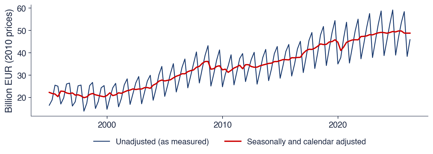

 TSA_ch0_examples