Bucharest University of Economic Studies IDA Institute Digital Assets Blockchain Research Center AI4EFin Artificial Intelligence for Energy Finance Romanian Academy, Institute for Economic Forecasting MSCA Digital Finance
The question of the chapter is what the whole course says about a time series. The answer is not a list of models but a sequence of questions: what does the series look like, is it stationary, how does it depend on its own past, is it seasonal, does its variance change, does it move together with other series, and how well can it be forecast. Each chapter of the course answers one of these questions, and the review puts them in the order in which they come up in a real analysis.
The route has three parts. The first goes through the course map, two slides per chapter and a summary of tests and models. The second walks through the Box–Jenkins method on Romanian inflation, step by step. The third describes the team project. Chapters 11–14 are for self-study and appear in the review only through their main ideas and their link with the core of the course.
In brief
Question: what does the whole course say about a time series, and how is it examined?
The first three outcomes concern the course as a whole. Placing a chapter on the road from description to forecasting means knowing which question the previous chapter left open and which new tool settles it: for example, the unit-root tests of Chapter 3 exist because the ARMA models of Chapter 2 assume a stationary series. For each chapter three things are worth keeping: the key formula, the main empirical fact from the course data and the mistake that comes up most often in applications.
The other outcomes are practical. The Box–Jenkins method ties transformation, testing, identification, estimation, checking and forecasting into a single analysis. Reading software output, estimates, tests and correlograms, needs the same structure every time: which hypothesis is tested, what the statistic shows and what the decision means for the series, in three to five sentences. The last outcome concerns the team project, its oral defence and the declaration of the use of artificial intelligence (AI) tools.
In brief
Place every chapter on the path from describing a series to modelling and forecasting it
Recall the key formula, the key empirical fact and the most common mistake of each chapter
Choose the right test or model for a given question about a time series
Run the Box–Jenkins method on a real series: transform, test, identify, estimate, check, forecast
Read software output (estimates, tests, correlograms) and interpret it in three to five sentences
Plan the team project, its oral defence and the declaration of AI use
The chapter's Quantlets hold the code of the Box–Jenkins case on the HICP: every table and every chart of that section can be rebuilt from the data. The course notebook gathers the whole course in a single file that runs in Google Colab. The chapter quiz has 20 questions drawn from all chapters and helps to see which ideas need rereading.
Self-assessment: the quiz of this chapter, 20 questions drawn from all chapters
Fifteen chapters have looked at a time series from different angles: its components, stationarity, dependence on its own past, unit roots, seasonality, variance that changes over time, links with other series, long memory, machine-learning methods and hidden states. Each chapter brought its own formulas, its own tests and its own pitfalls. The question of this chapter is what remains of all this when a real series has to be analysed from start to finish: which question comes first, which tool answers it and how the result is read.
The chapter has two parts. The first reviews the course: a map of the chapters, two slides per chapter with the key formulas, the main empirical facts and the most common mistakes, then a summary of tests and models that links each question about a series to the right test or model. The second part applies the Box–Jenkins method, in six steps, to the harmonised index of consumer prices (HICP) of Romania, from January 2005 to August 2026: transformation, tests, identification, estimation, residual checks and forecasting.
The example shows why the steps cannot be skipped. The model suggested by the correlogram fails the residual checks, and the chosen model, although it has the smallest forecast errors on the test sample, is not statistically separated from the naive methods over 24 months. The largest errors come from tax decisions and energy prices, which no univariate model can anticipate.
HICP of Romania, January 2005 – August 2026. Top: the index, 2015 = 100. Bottom: monthly inflation \(100\Delta\ln P_t\) (bars) and annual inflation \(100\Delta_{12}\ln P_t\) (red line), in percent.
What you will be able to do
Place each chapter of the course on the road from describing a series to modelling and forecasting it.
Recall the key formula, the main empirical fact and the most common mistake of each chapter.
Choose the right test or model for a given question about a time series.
Apply the Box–Jenkins method to a real series and interpret each result in a few sentences.
Evaluate forecasts out of sample, against simple benchmarks, with the Diebold–Mariano test.
Chapter plan
The course mapHow the fifteen chapters connect and on which real series they were illustrated.
The diagram places the chapters on four rows. The first row, one series and its mean, runs from Chapter 0 (components and smoothing) to stationarity and the correlogram, to ARMA models, to unit roots and ARIMA, and to seasonality and forecast evaluation. The second row, the variance and several series, holds ARCH and GARCH volatility, VAR models and cointegration with the VECM. Red boxes mark this core, and red arrows show the main dependencies: ARMA leads both to ARIMA and to GARCH, and unit roots lead to cointegration.
The third row holds the extensions, Chapters 8–10: long memory starts from volatility, machine learning from the VAR, and state space from seasonality and forecasting. The last row, with dashed boxes, holds the self-study chapters. Each is built on a core chapter: foundation models on machine learning, spectral analysis on the correlogram and on long memory, LPPL bubbles on unit roots, and multivariate GARCH on GARCH and on the VAR.
Read from left to right, the map follows the order of an analysis: first the description, then the question whether the series is stationary, then a model for the mean, then one for the variance and, at the end, several series modelled together.
The table lists the series on which the methods were illustrated, with their source, the topic they illustrate and the chapters in which they appear. Most are Romanian. Romanian quarterly real GDP has a trend, seasonality, a unit root and regime changes, so it serves in Chapters 0–4 and in Chapter 10. Monthly HICP inflation illustrates persistence, seasonality and long memory, and ROBOR 3M (Romanian Interbank Offer Rate) and unemployment enter, together with growth and inflation, a VAR for the Romanian economy.
The EUR/RON exchange rate is the example of a random walk that is hard to beat in forecasting. The daily stock indices BET, S&P 500 and DAX illustrate volatility clustering and spillover between markets. Electricity consumption, daily and hourly, has multiple seasonality and suits machine-learning methods. The classic textbook series, the Nile, sunspots, bond yields and US GDP, allow the results to be compared with the literature.
In brief
Series
Source
Topic illustrated
Ch.
Romanian real GDP (quarterly)
Eurostat
trend, seasonality, a unit root, regimes
0–4, 10
Romanian HICP inflation (monthly)
Eurostat
persistence, seasonality, long memory
2–4, 8
ROBOR 3M, unemployment
Eurostat
a VAR for the Romanian economy
6
EUR/RON
BNR
a random walk that is hard to beat
0, 3, 5
BET, S&P 500, DAX (daily)
EODHD
volatility clustering, spillovers
1, 5, 6
electricity load (daily, hourly)
ENTSO-E
multiple seasonality, machine learning
4, 9
Nile, sunspots, US yields and GDP
statsmodels, FRED
the classic examples of the textbooks
1, 2, 7, 8, 10
Section summary
The map and the series show the same idea from two directions: the methods of the course form a road, from description to several series modelled together, and each method was learned on a series that makes it necessary.
A series decomposes into a trend \(T_t\), a seasonal component \(S_t\) and a remainder \(R_t\). In the additive model, \(y_t = T_t + S_t + R_t\), the seasonal amplitude is constant in the units of the series; in the multiplicative model, \(y_t = T_t S_t R_t\), it grows with the level. The logarithm turns the product into a sum, so a multiplicative model for \(y_t\) is an additive model for \(\ln y_t\). For this reason almost all the macroeconomic series of the course are analysed in logs.
Simple exponential smoothing (SES) updates a level with a weighted average of the new observation and the previous level:
An \(\alpha\) close to 1 follows the latest observation closely, and a small \(\alpha\) smooths heavily. Accuracy is measured by the MASE (mean absolute scaled error): the mean absolute error (MAE) of the forecast divided by the in-sample MAE of the seasonal naive method. A value below 1 means the method beats the naive benchmark; the scaling makes series with different units comparable.
In brief
Key formulas
additive \(y_t = T_t + S_t + R_t\) or multiplicative \(y_t = T_t S_t R_t\); the logarithm turns one into the other
SES \(\ell_t = \alpha y_t + (1 - \alpha)\ell_{t-1}\); MASE \(=\) MAE \(/\) MAE of the in-sample seasonal naive method
Notation
\(T_t\), \(S_t\), \(R_t\): the trend, the seasonal component and the remainder (the irregular part)
\(\ell_t\): the smoothed level at time \(t\); \(\alpha \in (0, 1)\): the weight of the newest observation; a large \(\alpha\) follows the data closely
MAE: the mean absolute error; MASE below 1: better than the seasonal naive method
Chapter 0: Introduction: components and exponential smoothing (2/2)
Romanian GDP has grown 2.3 times since 1995, that is 2.8% a year, and the seasonal component is large: the first quarter is about 23.8% below the trend and the fourth quarter 20.7% above it. For EUR/RON, the estimated smoothing parameter is \(\hat\alpha = 1.00\), so the best forecast is the last observed value, the behaviour of a random walk. For electricity consumption, the Holt–Winters method, which adds trend and seasonality, has a MASE of 0.51, against 0.82 for the naive method.
The first common mistake is judging a forecast on the data used for estimation: in sample, a more complex model almost always fits better, which says nothing about the future. The second is using the mean absolute percentage error (MAPE) for series that pass through zero, such as monthly inflation: dividing by values close to zero makes the error arbitrarily large. The third is an additive model for a seasonal swing that grows with the level, where the logarithm or the multiplicative model is the right choice.
In brief
Empirical facts
Romanian GDP grew 2.3 times since 1995 (2.8% a year); Q1 is about \(\ensuremath{-}23.8\%\) and Q4 \(+20.7\%\) around the trend
EUR/RON: \(\hat\alpha_{SES} = 1.00\), the last value is the best forecast; electricity: Holt–Winters MASE 0.51 against 0.82 for the naive method
Common mistakes
judging a forecast on the data used to fit it
MAPE for series that cross zero (monthly inflation); an additive model for a seasonal swing that grows with the level
Chapter 1: Stochastic processes and stationarity (1/2)
A process is weakly stationary if its mean is constant, \(E X_t = \mu\), and its autocovariance \(\mathrm{Cov}(X_t, X_{t+h}) = \gamma(h)\) depends only on the distance \(h\), not on the time \(t\). Stationarity makes estimation possible: if the properties of the series do not change over time, observations from different periods inform about the same parameters. The sample autocorrelation \(\hat\rho(h)\) is compared with the band \(\pm 1.96/\sqrt{T}\), the approximate 95% band for white noise.
The Ljung–Box test (Ljung and Box, 1978) combines the first \(m\) autocorrelations into one statistic:
A large value, that is a small p-value, rejects white noise. The random walk \(X_t = X_{t-1} + \varepsilon_t\) is the basic example of a non-stationary series: its variance, \(\mathrm{Var}(X_t) = t\sigma^2\), grows linearly in time, so there is no constant variance to estimate.
Ljung–Box \(Q^*(m) = T(T + 2)\sum_{h=1}^{m}\hat\rho(h)^2/(T - h) \sim \chi^2(m)\)Ljung and Box (1978); random walk \(\mathrm{Var}(X_t) = t\sigma^2\)
Notation
\(\mu\): the constant mean; \(\gamma(h)\): the autocovariance at lag \(h\), which depends only on \(h\); \(\hat\rho(h)\): the sample autocorrelation; \(T\): the number of observations
\(Q^*(m)\): the Ljung–Box statistic on the first \(m\) lags; a large value (a small p-value) rejects white noise
\(\sigma^2\): the variance of the random-walk shocks; \(\mathrm{Var}(X_t) = t\sigma^2\) grows with \(t\), so a random walk is not stationary
Chapter 1: Stochastic processes and stationarity (2/2)
Daily BET returns have a first-order autocorrelation of 0.11, and absolute returns have 0.40, both against a band of \(\pm 0.024\). The gap between the two numbers is one of the central ideas of the course: a series can be almost uncorrelated without being independent. The size of returns is predictable even when their sign is not, and this observation prepares the GARCH models of Chapter 5.
For Romanian GDP, the Box–Cox transformation has the estimated parameter \(\hat\lambda = 0.02\), practically the logarithm. One difference too many applied to a series that is already stationary gives a first-order autocorrelation of \(-0.54\): over-differencing introduces an artificial negative autocorrelation, the sign of a unit root in the MA part. The other common mistake is reading a single bar outside the band as a signal: at 20 lags, one falls outside the band by chance, even for white noise.
In brief
Empirical facts
BET returns: \(\hat\rho_1 = 0.11\), absolute returns \(\hat\rho_1 = 0.40\) (band \(\pm 0.024\)): uncorrelated is not independent
Romanian GDP: Box–Cox \(\hat\lambda = 0.02\), the logarithm; one difference too many gives \(\hat\rho_1 = \ensuremath{-}0.54\)
Common mistakes
reading one bar outside the band as a signal (one in twenty is outside by chance)
The ARMA\((p, q)\) model is written with the lag operator \(L\), defined by \(LX_t = X_{t-1}\):
\[\phi(L)(X_t - \mu) = \theta(L)\varepsilon_t,\]
(15.3)
where \(\phi(L)\) and \(\theta(L)\) are the AR and MA polynomials, of orders \(p\) and \(q\), and \(\varepsilon_t\) is white noise. The two simple cases give the identification patterns: an AR(1) has autocorrelations \(\rho(h) = \phi^h\), which decay geometrically, and an MA(1) has a single non-zero autocorrelation, \(\rho(1) = \theta/(1 + \theta^2)\), and cuts off after lag 1.
Among the candidate models we choose with information criteria. The Akaike criterion (Akaike, 1974),\(\mathrm{AIC} = -2\ln\hat{\mathcal{L}} + 2k\), and the Schwarz criterion (Schwarz, 1978),\(\mathrm{BIC} = -2\ln\hat{\mathcal{L}} + k\ln T\), start from the maximised log-likelihood and penalise the number \(k\) of parameters; smaller is better. The BIC penalty exceeds the AIC penalty as soon as \(\ln T > 2\), that is for \(T \ge 8\), so the BIC picks smaller models. After estimation, the Ljung–Box test on the residuals uses \(m - p - q\) degrees of freedom, because the estimated parameters absorb part of the autocorrelation.
\(L\): the lag operator, \(LX_t = X_{t-1}\); \(\phi(L)\), \(\theta(L)\): the AR and MA polynomials of orders \(p\) and \(q\); \(\varepsilon_t\): white noise
\(\ln\hat{\mathcal{L}}\): the maximised log-likelihood; \(k\): the number of estimated parameters; a smaller AIC or BIC is better
BIC penalises parameters more than AIC, since \(\ln T > 2\) for \(T \ge 8\)
For Romanian annual GDP growth, the BIC chooses an MA(3). The explanation is the construction of the series: growth on the same quarter of the previous year is computed over overlapping four-quarter windows, and the overlap creates a dependence that stops after three lags. The residuals of the model have a Ljung–Box p-value of 0.37, so the test does not separate the remaining autocorrelation from noise. Romanian inflation fits an AR(2) with \(\hat\phi_1 + \hat\phi_2 = 0.976\), very close to a unit root, and sunspots have an AR(2) cycle of 10.6 years.
The first common mistake is reading the AR order from the ACF: for an AR process it is the PACF that cuts off, not the ACF. The second is the Ljung–Box test on residuals with \(m\) degrees of freedom instead of \(m - p - q\), which makes the test too lenient. The third is a common factor in \(\phi(L)\) and \(\theta(L)\): if the two polynomials share a root, it cancels, and the model has parameters that cannot be identified.
In brief
Empirical facts
annual growth of Romanian GDP: MA(3) by BIC, a product of overlapping quarters; residual Ljung–Box \(p = 0.37\)
Romanian inflation: AR(2) with \(\hat\phi_1 + \hat\phi_2 = 0.976\), close to a unit root; sunspots: an AR(2) cycle of 10.6 years
Common mistakes
reading the AR order from the ACF (it is the PACF that cuts off for an AR)
Ljung–Box on residuals with \(m\) instead of \(m - p - q\) degrees of freedom; a common factor in \(\phi(L)\) and \(\theta(L)\)
and tests \(H_0\):\(\gamma = 0\), that is a unit root. The lagged differences, with coefficients \(\delta_j\), remove the autocorrelation of the errors. Under \(H_0\) the \(t\) statistic of \(\gamma\) does not follow the Student distribution but a distribution of its own, with more negative critical values. The KPSS test (Kwiatkowski et al., 1992) reverses the hypotheses: \(H_0\) is stationarity. Used together, the two tests give four combinations of decisions, two of them clear and two inconclusive.
The ARIMA\((p, d, q)\) model applies an ARMA to the series differenced \(d\) times:
\[\phi(L)(1 - L)^d y_t = c + \theta(L)\varepsilon_t.\]
(15.5)
When \(d \ge 1\), the variance of the forecast error grows with the horizon \(h\) without bound, because shocks have a permanent effect on the level. This is the practical difference between a stochastic and a deterministic trend: around a deterministic trend, forecast intervals keep a bounded width.
For the log of Romanian GDP, the ADF statistic is \(\tau = -2.31\), with p-value 0.43, and the 5% critical value is \(-3.45\); the unit root is not rejected. For growth, \(\tau = -10.77\) rejects clearly. The resulting model is an ARIMA(0,1,0) with a drift of 0.81% per quarter: a random walk with average growth. The experiment of Granger and Newbold (1974) shows the danger of regressions between integrated series: for two independent random walks, the \(t\) statistic of the slope is significant in 90% of regressions.
The ADF test has low power: for \(\phi = 0.95\) and \(T = 100\), it rejects the unit root in only 12.5% of cases. Non-rejection therefore does not prove a unit root; it only shows that the data cannot separate it from a root close to 1. The other common mistakes are Student or Normal critical values for the ADF statistic and a regression in levels between \(I(1)\) series without a cointegration test.
In brief
Empirical facts
log Romanian GDP: \(\tau = \ensuremath{-}2.31\) (\(p = 0.43\), 5% critical value \(\ensuremath{-}3.45\)); growth: \(\tau = \ensuremath{-}10.77\); ARIMA(0,1,0) with drift 0.81% a quarter
two independent random walks: a significant \(t\) in 90% of regressions Granger and Newbold (1974); ADF power only 12.5% for \(\phi = 0.95\), \(T = 100\)
Common mistakes
Student or Normal critical values for the ADF statistic
reading a non-rejection as proof of a unit root; a regression in levels of \(I(1)\) series without a cointegration test
Section summary
The first four chapters give the working order for a single series: the transformation that stabilises the variance, the tests that decide how many times to difference, the correlogram that suggests the ARMA orders and the information criteria that choose among candidates, with the residuals checked at the end.
Chapters 4–7: seasonality, volatility, VAR, VECM
Chapters 4–7 add seasonality and forecast evaluation, then move from the mean to the variance and from one series to several.
where \(s\) is the length of the season, 12 for monthly data, \(\Phi\) and \(\Theta\) are the seasonal polynomials and \(D\) is the number of seasonal differences \((1 - L^s)\). The airline model, \((0,1,1)(0,1,1)_s\), with one ordinary difference, one seasonal difference and one MA term in each part, is the classic starting point for monthly series with trend and seasonality.
To compare two forecasts we use the Diebold–Mariano test (Diebold and Mariano, 1995). For each period the loss differential \(d_t = L(e_{1t}) - L(e_{2t})\) is computed, for example the difference of squared errors, and the statistic is the mean \(\bar d\) divided by its standard error, \(\bar d/\sqrt{\hat V/n}\), with \(\hat V\) the long-run variance of \(d_t\). Under equal accuracy the statistic is approximately \(N(0, 1)\), so \(|\mathrm{DM}| > 1.96\) rejects at 5%. The correction of Harvey, Leybourne and Newbold (1997) (HLN) adjusts the statistic for small samples and compares it with the Student distribution.
\(s\): the season length (12 for monthly data); \(\Phi(L^s)\), \(\Theta(L^s)\): the seasonal AR and MA polynomials; \(D\): the number of seasonal differences \((1 - L^s)\)
\(e_{1t}\), \(e_{2t}\): the errors of the two forecasts; \(L(\cdot)\): the loss, e.g. the square; \(d_t\): the loss differential; \(\bar d\): its mean; \(\hat V\): its estimated long-run variance; \(n\): the number of forecasts
under equal accuracy DM is approximately \(N(0, 1)\): \(|\mathrm{DM}| > 1.96\) rejects at 5%
For the airline passenger series, the airline model has a MAPE of 8.5%, against 15.5% for the seasonal naive method. Orthodox Easter, which does not fall in the same month every year, raises Romanian food sales by about 5.9%; such a calendar effect enters the model as an explanatory variable, not through seasonal differencing. For daily electricity consumption, dynamic harmonic regression (DHR), with Fourier terms for the annual seasonality, has a MASE of 0.89, against 1.28 for the seasonal naive method.
The first common mistake is comparing AICc across models with different \(d\) or \(D\): differencing changes the data on which the likelihood is computed, so the criteria are no longer comparable. The second is judging forecasts at a single origin, which can hinge on one unusual episode; rolling origins give a more stable picture. The third is using seasonally adjusted data in a SARIMA model that has to forecast the raw data.
In brief
Empirical facts
airline passengers: MAPE 8.5% for the airline model against 15.5% for the seasonal naive method
Orthodox Easter raises Romanian food sales by about 5.9%; daily load: DHR MASE 0.89 against 1.28 (seasonal naive)
Common mistakes
comparing AICc of models with different \(d\) or \(D\)
judging forecasts at a single origin; seasonally adjusted data in a SARIMA forecast of raw data
Chapter 5: Conditional volatility: ARCH and GARCH (1/2)
with \(\omega > 0\),\(\alpha \ge 0\),\(\beta \ge 0\). The parameter \(\alpha\) measures the reaction to shocks and \(\beta\) the persistence. If \(\alpha + \beta < 1\), the variance reverts to the long-run level \(\bar\sigma^2 = \omega/(1 - \alpha - \beta)\), and a volatility shock halves in \(h_{1/2} = \ln 0.5/\ln(\alpha + \beta)\) periods. The closer \(\alpha + \beta\) is to 1, the more persistent the volatility.
The ARCH-LM test checks whether the variance changes: \(\varepsilon_t^2\) is regressed on \(q\) of its lags, and \(nR^2\) is \(\chi^2(q)\) under constant variance. The model is then used for the risk of loss. With the conditional mean \(\mu\), the forecast volatility \(\sigma_{t+1}\) and the 1% quantile \(q_{0.01}(z)\) of the standardised innovations, VaR 1% is
\(\sigma_t^2\): the conditional variance; \(\varepsilon_{t-1}\): yesterday's shock; \(\omega > 0\): the constant; \(\alpha \ge 0\): the reaction to shocks; \(\beta \ge 0\): the persistence
\(\bar\sigma^2\): the long-run variance, defined only if \(\alpha + \beta < 1\); \(h_{1/2}\): the half-life of a volatility shock
ARCH-LM: \(R^2\) of the regression of \(\varepsilon_t^2\) on \(q\) of its lags, \(n\) observations; \(q_{0.01}(z)\): the 1% quantile of the standardised innovations \(z_t\); \(\mu\): the conditional mean
Chapter 5: Conditional volatility: ARCH and GARCH (2/2)
A GARCH(1,1) with Student innovations has \(\alpha + \beta = 0.995\) for the S&P 500, with a half-life of 131 days, and \(0.991\) for the BET, with 74 days: volatility is very persistent on both markets. The GJR model, which adds a term for negative shocks, has \(\hat\gamma = 0.21\) for the S&P 500, with a \(t\) statistic of 10.0; price falls raise volatility more than rises of the same size, the leverage effect. Kurtosis is 13.7 for returns and 5.0 for the standardised residuals: the model explains much of the fat tails, but not all.
The common mistakes concern the formulas. The half-life is not \(1/(1 - \alpha - \beta)\) but \(\ln 0.5/\ln(\alpha + \beta)\). The long-run variance does not exist when \(\alpha + \beta \ge 1\), so it must not be reported. In the course, the VaR level is the tail probability and VaR is a positive loss: it is written VaR 1%, never "VaR 99%", and a negative value signals a sign error.
In brief
Empirical facts
GARCH(1,1)-\(t\): \(\alpha + \beta = 0.995\) for the S&P 500 (half-life 131 days), \(0.991\) for the BET (74 days)
S&P 500: GJR \(\hat\gamma = 0.21\) (\(t = 10.0\)); kurtosis 13.7 for returns, 5.0 for standardised residuals
Common mistakes
the half-life written as \(1/(1 - \alpha - \beta)\); a long-run variance reported when \(\alpha + \beta \ge 1\)
“VaR 99%” or a negative VaR: the course writes VaR 1%, a positive loss
The matrices \(\bA_i\) are \(K \times K\). Written as a VAR(1) of dimension \(Kp\), through the companion matrix, the model is stable if all eigenvalues of that matrix lie inside the unit circle; then the effect of any shock dies out over time.
Granger causality (Granger, 1969) asks whether the lags of a variable \(x\) improve the forecast of \(y\), given the history of \(y\). The test compares the residual sum of squares without the lags of \(x\),\(RSS_R\), with the one with the lags of \(x\),\(RSS_U\):
Impulse response functions (IRF) and the forecast error variance decomposition (FEVD) need uncorrelated shocks, usually obtained by a Cholesky decomposition, which depends on the ordering of the variables.
In brief
Key formulas
VAR\((p)\): \(\bY_t = \bc + \bA_1\bY_{t-1} + \dots + \bA_p\bY_{t-p} + \bepsilon_t\)Sims (1980); stable if all eigenvalues of the companion matrix are inside the unit circle
Granger \(F = [(RSS_R - RSS_U)/p]\,/\,[RSS_U/(T - Kp - 1)]\)Granger (1969); IRF and FEVD with a Cholesky ordering
Notation
\(\bY_t\): the vector of the \(K\) variables; \(\bc\): the constants; \(\bA_i\): the \(K \times K\) coefficient matrices of lag \(i\); \(\bepsilon_t\): the vector of shocks
the companion matrix writes the VAR(\(p\)) as a VAR(1) of dimension \(Kp\)
\(RSS_R\), \(RSS_U\): the residual sums of squares without and with the lags of the tested variable; \(p\): the number of restrictions
A VAR(2) for Romania, with growth, inflation and ROBOR 3M, shows that growth Granger-causes ROBOR: the \(F\) statistic is 7.26, with p-value 0.001. The lags of growth thus carry information about the future interbank rate beyond the rate's own past. The spillover index between the S&P 500, the DAX and the BET, built from the FEVD, averages 26.4% and reaches 57.5% on 17 March 2020: in crises, a much larger share of each market's variation comes from shocks to the others.
The first common mistake is reading Granger causality as causality in the economic sense; the test only measures additional predictability, and an omitted third variable can produce the result. The second is reporting IRFs without the Cholesky ordering behind them, although the responses can change with the ordering. The third is using too many lags on a short sample: the number of parameters grows with \(K^2p\).
In brief
Empirical facts
Romanian VAR(2) of growth, inflation and ROBOR 3M: growth Granger-causes ROBOR, \(F = 7.26\), \(p =\) 0.001
spillovers among the S&P 500, DAX and BET: 26.4% on average, 57.5% on 17 March 2020
Common mistakes
reading Granger causality as causality (it is extra predictability)
IRFs reported without the ordering behind them; too many lags for a short sample
Two \(I(1)\) series are cointegrated if a linear combination of them is stationary. The Engle–Granger method (Engle and Granger, 1987) estimates the relation by OLS in levels, then applies an ADF test to the residuals, with MacKinnon critical values, more negative than the Dickey–Fuller ones, because the residuals come from an estimated regression. In the error correction model, the coefficient \(\gamma < 0\) on last period's disequilibrium is the speed of adjustment, and the half-life of a deviation is \(\ln 0.5/\ln(1 + \gamma)\).
The vector error correction model (VECM) writes the differences as functions of last period's disequilibria and of the short-run dynamics:
The columns of \(\beta\) are the equilibrium relations, and \(\alpha\) says how fast each variable reacts to disequilibrium. The trace test of Johansen (1991), with the statistic \(-T\sum_{i>r}\ln(1 - \hat\lambda_i)\), tests the ranks \(r = 0, 1, \dots\) in turn; the first rank that is not rejected is the cointegration rank.
In brief
Key formulas
Engle–Granger: OLS in levels, then ADF on residuals with MacKinnon critical values Engle and Granger (1987); ECM half-life \(\ln 0.5/\ln(1 + \gamma)\)
ECM: \(\gamma < 0\) is the speed of adjustment towards equilibrium
\(\beta\): the cointegrating vectors (the equilibrium relations); \(\alpha\): the adjustment coefficients; \(\Gamma_i\): the short-run dynamics; \(\mathbf u_t\): the shocks
\(\hat\lambda_i\): the estimated eigenvalues, in decreasing order; \(r\): the tested cointegration rank; a trace above its critical value rejects rank \(r\)
For US bond yields at 1, 5 and 10 years, the trace statistic is 54.6 for \(r = 0\), above the critical value of 29.8, and 3.12 for \(r \le 2\), below the critical value of 3.84: the cointegration rank is 2. Three rates with two equilibrium relations share a single common stochastic trend, the general level of interest rates. The half-life of the error correction for the long rate is 20.8 months.
Purchasing power parity (PPP) for the leu is not supported: the ADF test for the real exchange rate has p-value 0.24, so the unit root is not rejected. For pairs trading on the Bucharest Stock Exchange, the Sharpe ratio of the strategy is 0.15 before costs and 0.05 after. The common mistakes are Dickey–Fuller critical values for Engle–Granger residuals and a VAR in differences for cointegrated series, which omits the error correction term and with it the long-run information.
In brief
Empirical facts
US yields at 1, 5 and 10 years: trace 54.6 \(>\) 29.8 for \(r = 0\), 3.12 \(<\) 3.84 for \(r \le 2\): rank 2; long-rate ECM half-life 20.8 months
PPP for the leu: ADF \(p = 0.24\) on the real exchange rate, not stationary; pairs trading on the BVB: Sharpe 0.15 gross, 0.05 net
Common mistakes
Dickey–Fuller critical values for Engle–Granger residuals (they must be more negative)
a VAR in differences for cointegrated series (it omits the error correction term)
Section summary
Chapters 4–7 extend the single-series model in three directions: seasonality, with SARIMA and proper forecast evaluation; the variance, with GARCH and VaR; and several series, with the VAR, Granger causality and, when the series are integrated and tied by an equilibrium, the VECM.
Chapters 8–10: long memory, machine learning, state space
Chapters 8–10 extend the core of the course with long memory, machine-learning methods and models with hidden states.
Between \(d = 0\), a stationary short-memory process, and \(d = 1\), a unit root, there are fractional values of \(d\)(Granger and Joyeux, 1980; Hosking, 1981). The operator \((1 - L)^d\) expands into an infinite series of lags, with weights given by the recursion
For \(0 < d < 1/2\) the process is stationary, but the autocorrelations decay hyperbolically, \(\rho(k) \sim Ck^{2d-1}\), not exponentially as for an ARMA: a shock has an effect over hundreds of periods.
The Hurst exponent is \(H = d + 1/2\), above 0.5 for long memory; in the course it is estimated with the rescaled range (R/S) statistic. The process is stationary for \(d < 1/2\) and mean-reverting for \(d < 1\), even though its variance is then no longer finite. The GPH and local Whittle estimators use only the lowest \(m\) frequencies of the periodogram, where long memory leaves its mark; the choice of \(m\) changes the estimate.
stationary for \(d < 1/2\), mean-reverting for \(d < 1\); GPH and local Whittle use the lowest \(m\) frequencies
Notation
\(d\): the order of fractional integration; \(\pi_k\): the weight of lag \(k\) in the expansion of \((1 - L)^d\)
\(C > 0\): a constant; \(\rho(k) \sim Ck^{2d-1}\): the ACF decays hyperbolically, not exponentially
\(H\): the Hurst exponent, above 0.5 for long memory, estimated here by the rescaled-range (R/S) statistic; \(m\): the number of low frequencies used by GPH and local Whittle
For Romanian monthly inflation, an ARFIMA(0,\(d\),0) with \(\hat d = 0.31\) and standard error 0.05 beats the ARMA models by both AIC and BIC: one fractional parameter describes the persistence better than several AR and MA terms. For the S&P 500, the Hurst exponent estimated by R/S is 0.53 for returns, close to 0.5, and 0.86 for absolute returns: the long memory is in volatility, not in returns.
The Nile shows the main pitfall of the chapter. Over the whole series \(\hat d = 0.40\), but after removing the 1898 break, when the level of the series shifts, the estimate becomes \(-0.17\). A break or a regime change produces in the correlogram the same slow decay as long memory. The other common mistakes are reporting a single bandwidth \(m\) and confusing long memory in returns with long memory in volatility.
In brief
Empirical facts
Romanian monthly inflation: ARFIMA(0,\(d\),0) with \(\hat d = 0.31\) (SE 0.05) beats ARMA by AIC and BIC
S&P 500: \(H\) (R/S) 0.53 for returns, 0.86 for \(|r_t|\); the Nile: \(\hat d = 0.40\), but \(\ensuremath{-}0.17\) after the break of 1898
Common mistakes
a break or a regime change read as long memory
one bandwidth \(m\) only; long memory in returns confused with long memory in volatility
Machine-learning methods usually forecast directly: for each horizon \(h\) a separate function is estimated of the last \(p\) values and of regressors known in advance, such as the calendar,
Penalised regressions control complexity: ridge adds the term \(\lambda\sum\beta_j^2\) to the sum of squared errors and shrinks all coefficients, while lasso adds \(\lambda\sum|\beta_j|\) and sets some of them to zero, so it selects predictors.
The bias–variance decomposition explains why a more flexible model is not automatically better: the mean squared forecast error for a new observation is
Flexibility reduces the bias and raises the variance, and \(\sigma^2\) cannot be removed by any model. Validation must respect the order of time: walk-forward validation estimates on the past and evaluates on the period right after, then moves forward.
For the S&P 500, the same model has \(R^2 = 0.37\) with random \(k\)-fold cross-validation and \(-0.39\) with walk-forward validation. The difference is leakage: the random split lets the model learn from observations that come after the ones it forecasts. For the sign of returns, the majority class is right on 54.4% of days and a boosting model on only 52.5%. For daily electricity consumption, ridge has a MASE of 0.90 and an LSTM (long short-term memory) network 1.16, in line with the conclusion of the M4 competition (Makridakis, Spiliotis and Assimakopoulos, 2020) that complex methods do not automatically beat simple ones.
The common mistakes are random cross-validation and scaling the variables on the whole sample, both forms of look-ahead. Decision trees cannot extrapolate: applied to trending levels, their forecasts stay within the range of the training values, so the trend must be removed first. Every comparison needs a simple benchmark, the naive or seasonal naive method.
In brief
Empirical facts
S&P 500, the same model: \(R^2 = 0.37\) with random \(k\)-fold, \(\ensuremath{-}0.39\) walk-forward: leakage
A state space model has two equations: a measurement equation, which links the observation to a hidden state, and a transition equation, which describes how the state evolves:
The Kalman filter (Kalman, 1960) updates the state estimate when a new observation arrives: \(a_{t|t} = a_t + K_tv_t\), where \(v_t = y_t - Za_t\) is the prediction error and the gain \(K_t = P_tZ'F_t^{-1}\) is the weight of this surprise. When the predicted state is uncertain, \(P_t\) large, the gain is large and the filter relies more on the observation.
In the Markov switching model (Hamilton, 1989), the parameters depend on an unobserved regime that moves from one state to another with probabilities \(p_{ij}\). The expected duration of regime \(i\) is \(1/(1 - p_{ii})\), and with two regimes the long-run share of regime 1 is
\(\alpha_t\): the hidden state (e.g. the level); \(Z\), \(T\), \(R\): known system matrices; \(\varepsilon_t\), \(\eta_t\): the measurement and state noise
\(a_t\), \(P_t\): the predicted state and its variance; \(v_t = y_t - Za_t\): the prediction error, with variance \(F_t\); \(K_t\): the Kalman gain, the weight of the surprise
\(p_{ii}\): the probability of staying in regime \(i\); \(\pi_1\): the long-run share of regime 1
Chapter 10: State space models, Kalman filter and Markov switching (2/2)
For the Nile, the local level model has the estimated signal-to-noise ratio \(\hat q = \hat\sigma^2_\eta/\hat\sigma^2_\varepsilon = 0.097\): the level changes little relative to the measurement noise. The Kalman gain converges to \(\bar K = 0.267\), which is exactly the weight \(\alpha\) of the exponential smoothing of Chapter 0; exponential smoothing is the Kalman filter of the local level model. For US GDP, the estimated regimes match the NBER (National Bureau of Economic Research) recession dates in 90% of quarters; for Romanian GDP, the stable regime lasts 15.2 quarters on average and the volatile one 11.2.
The first common mistake is using the smoothed probabilities, which use the whole sample, as if they had been known in real time; for real-time decisions the filtered probabilities matter. The second is writing the duration as \(p_{ii}/(1 - p_{ii})\) instead of \(1/(1 - p_{ii})\). The third concerns the Hodrick–Prescott filter: the last value of the deviation from trend is heavily revised when new data arrive, so it is not a real-time estimate.
In brief
Empirical facts
the Nile: \(\hat q = \hat\sigma^2_\eta/\hat\sigma^2_\varepsilon = 0.097\), steady-state gain \(\bar K = 0.267\), the weight of exponential smoothing
US GDP: the regimes match the NBER dates in 90% of quarters; Romanian GDP: stable regime 15.2 quarters, volatile 11.2
Common mistakes
smoothed probabilities used as if known in real time
durations written as \(p_{ii}/(1 - p_{ii})\); the last value of the HP gap read as a real-time estimate
Section summary
The extensions have the same structure as the core: each introduces a new model for a question the earlier models could not handle and comes with a pitfall of its own, a break mistaken for long memory, look-ahead in validation and future information in smoothed probabilities.
Chapters 11–14: self-study
The last four chapters are for self-study. The review gives their main ideas and their link with the core of the course.
Chapter 11: Foundation models for time series (self-study)
Foundation models are transformer models pre-trained on a very large number of series. The values of a series are turned into tokens, by scaling and quantisation, or split into consecutive segments (patching), and the model learns to continue the sequence. Chronos, TimesFM, Moirai and Lag-Llama can forecast zero-shot, that is on a series they did not see in training, without any further estimation, or they can be adapted by fine-tuning.
The link with the core is twofold. Such a model is a global model, estimated on many series at once, like the machine-learning models of Chapter 9. Its forecasts are evaluated like any forecast in Chapter 4: the same test sample, the MASE, scores for probabilistic forecasts and comparison with simple benchmarks.
In brief
Key ideas
transformers pre-trained on many series: tokenisation and patching of the values
Chronos, TimesFM, Moirai, Lag-Llama: zero-shot forecasts and fine-tuning
a fair comparison: the same test sample, MASE, probabilistic scores, simple benchmarks
Link with the core of the course
a global model of many series (Chapter 9); judged like any forecast (Chapter 4)
Spectral analysis describes a stationary series by the frequencies that make it up. The Fourier transform decomposes the series into sinusoids, the periodogram \(I(\nu_j)\) measures how much of the variance falls on each Fourier frequency \(\nu_j\), and the spectral density is the theoretical version of the periodogram. The raw periodogram fluctuates a lot, so it is smoothed, for example by Welch's method. Filters, such as Hodrick–Prescott, keep some frequencies and remove the others, which turns the business cycle into a band of frequencies.
The spectrum holds the same information as the autocovariance function of Chapter 1, ordered by frequency instead of by lag. The long memory of Chapter 8 appears as a pole of the spectral density at frequency zero. Coherence measures the link between two series at each frequency, and wavelets allow the study of frequencies that change over time.
In brief
Key ideas
the Fourier transform, the periodogram \(I(\nu_j)\) and the spectral density
smoothed periodograms (Welch), filters (Hodrick–Prescott) and business cycles
coherence between two series; wavelets as a time–frequency tool
Link with the core of the course
the same information as the ACF, by frequency (Chapter 1); the spectral pole of long memory (Chapter 8)
Chapter 13 describes speculative bubbles as a super-exponential growth of prices, faster than any exponential growth. The LPPLS (log-periodic power law singularity) model combines a power law leading to a critical time with ever faster log-periodic oscillations. Estimation needs filter conditions that remove fits without economic meaning, and many estimation windows are combined into a confidence indicator, applied to historical bubbles and crashes.
The link with the core is the Dickey–Fuller test of Chapter 3, used the other way round: explosive-root tests look for an autoregressive root above 1, in the right tail. The second link is the volatility before crashes, studied with the tools of Chapter 5.
In brief
Key ideas
bubbles as super-exponential growth of prices
the LPPLS model: power law plus log-periodic oscillations; estimation and filter conditions
the LPPLS confidence indicator on historical bubbles and crashes
Link with the core of the course
explosive roots, the opposite of unit roots (Chapter 3); volatility before crashes (Chapter 5)
Chapter 14 moves from the volatility of one series to the covariance matrix of several series, which changes over time. The main problem is the number of parameters, which grows very fast with the number of series. The VEC and BEKK models model the covariances directly, with many restrictions, while the CCC (constant conditional correlation) and DCC (dynamic conditional correlation) models separate the individual volatilities from the correlations. The DCC is estimated in two steps: first a GARCH for each series, then the correlation dynamics on the standardised residuals.
The results are dynamic correlations, the variance of a portfolio and the portfolio's VaR 1%. The link with the core is direct: each series has its own GARCH from Chapter 5, and the multivariate view, with coefficient matrices and a number of parameters that grows fast, is that of the VAR model of Chapter 6.
In brief
Key ideas
time-varying covariances and correlations; the number of parameters grows fast
VEC, BEKK, CCC and DCC; estimation of DCC in two steps
dynamic correlations, portfolio variance and VaR 1%
Link with the core of the course
GARCH for each series (Chapter 5) and the multivariate view of the VAR (Chapter 6)
The self-study chapters use the same ideas as the core in new settings: out-of-sample evaluation for foundation models, the autocovariance read by frequency, the Dickey–Fuller test in the right tail and GARCH extended to several series.
Summary of tests and models
The summary links each question about a series to the test that answers it and to the decision that follows.
Tests and models (1/2): univariate series and the mean
The table has four columns: the question, the tool, the decision and the chapter. The first two rows concern stationarity and the type of trend. The plot and the ACF give a first impression, and ADF and KPSS decide: when ADF rejects the unit root and KPSS does not reject stationarity, the series is stationary. With a trend in the regression, the same pair of tests decides between a deterministic trend, removed by regression, and a stochastic one, removed by differencing.
Seasonality shows in the seasonal plot and in the ACF at lags \(s\) and \(2s\); the OCSB and HEGY tests decide whether a seasonal difference \(\Delta_s\) is needed or whether dummy variables and Fourier terms are enough. The ARMA order is identified from the ACF and PACF and chosen with AIC and BIC: the model with the smallest BIC among those with white-noise residuals. Residuals are checked with Ljung–Box with \(m - k\) degrees of freedom and with Jarque–Bera for Normality. The last row compares forecasts: a test sample, rolling origins, the MASE and the Diebold–Mariano test; if the p-value is above 0.05, the two forecasts are not statistically separated.
In brief
Question
Tool
Decision
Ch.
Is the series stationary?
plot, ACF; ADF and KPSS
ADF rejects, KPSS does not: stationary
1, 3
Trend: deterministic or stochastic?
ADF and KPSS with a trend
detrend, or difference
3
Is there seasonality?
seasonal plot, ACF at \(s\), \(2s\); OCSB, HEGY
\(\Delta_s\), or dummies and Fourier terms
4
Which ARMA?
ACF, PACF; AIC, BIC
smallest BIC with white-noise residuals
2
Are the residuals adequate?
Ljung–Box on \(m - k\) df; Jarque–Bera
\(p > 0.05\): no autocorrelation left
2
Which forecast is better?
test sample, rolling origins; MASE, DM
DM \(p < 0.05\); otherwise a tie
0, 4
Tests and models (2/2): variance, multivariate series and extensions
The second part starts with the variance. The Ljung–Box test on squared returns \(r_t^2\) and the ARCH-LM test check whether the variance changes; if they reject, the suitable models are a GARCH(1,1) with Student innovations and the GJR, for asymmetry. For several series, the question whether \(x\) helps to forecast \(y\) is answered by the Granger causality \(F\) test in a VAR. The effect of a shock is measured by IRFs and the FEVD, with bootstrap bands and several Cholesky orderings, to see how much the results depend on the ordering. A long-run equilibrium is tested with Engle–Granger or Johansen, and the VECM gives the relations \(\beta\), the adjustment coefficients \(\alpha\) and the half-life.
The last rows concern the extensions. Long memory is estimated with GPH, local Whittle and ARFIMA, with several values of \(m\) and a check for breaks. For many predictors and nonlinear effects, ridge, lasso, trees and boosting are evaluated walk-forward, against a benchmark. For a hidden level or regime, the Kalman filter and Markov switching give filtered estimates for real time and smoothed ones for history.
Transformations are always written in the same form. The logarithm is multiplied by 100, so that differences are approximately percentages: \(100\Delta\ln y_t\) is the growth on the previous period, and \(100\Delta_{12}\ln y_t\) for monthly data and \(100\Delta_4\ln y_t\) for quarterly data are the annual rates. In EViews output, "DLOG(IPC,1,12)" means the ordinary difference of the seasonal difference of the logarithm, \(\Delta\Delta_{12}\ln\) IPC.
Every test is reported the same way: the null hypothesis, the statistic, its distribution under \(H_0\), the critical value or the p-value and the decision at 5%, followed by one sentence on what the decision means for the series. The information criteria AIC, AICc and BIC are compared only on the same sample and for the same \(d\) and \(D\), and forecasts are judged out of sample, against the naive and seasonal naive methods. For risk, the level is the tail probability: VaR 1% is a positive loss, \(\mathrm{VaR}_\alpha = -q_\alpha\), where \(q_\alpha\) is the \(\alpha\)-quantile of the return.
“DLOG(IPC,1,12)” in EViews output is \(\Delta\Delta_{12}\ln\) IPC
Tests
state \(H_0\), the statistic, its distribution, the critical value or \(p\)-value, the decision at 5%
then one sentence on what the decision means for the series
Model choice
AIC, AICc and BIC only on the same sample and the same \(d\), \(D\)
forecasts are judged out of sample, against the naive and seasonal naive methods
Risk
the level is the tail probability: VaR 1%, a positive loss, \(\mathrm{VaR}_\alpha = -q_\alpha\), \(q_\alpha\): the \(\alpha\)-quantile of the return
Section summary
The summary turns the course into a list of questions with verifiable answers. A good analysis goes through them in order, reports each test with its null hypothesis and its decision, and respects the conventions for transformations, model comparison and risk reporting.
Box–Jenkins from start to finish: Romanian inflation
The section applies the Box–Jenkins method, in six steps, to the Romanian HICP. Each step uses tools from earlier chapters, and each decision rests on a reported result.
The method of Box, Jenkins and Reinsel (2008) is a loop, not a linear recipe. The first step is the plot and the transformation: the logarithm to stabilise the variance, the ordinary difference \(\Delta\) for the trend and the seasonal difference \(\Delta_{12}\) for seasonality. The second step applies the ADF and KPSS tests to each transformation. The third identifies the orders from the ACF and PACF of the stationary series, and the fourth estimates several candidate SARIMA models by maximum likelihood and compares them with AICc and BIC.
The fifth step checks the residuals: autocorrelation with Ljung–Box, Normality with Jarque–Bera, and outliers. If the check fails, the analysis goes back to step 3. The sixth step forecasts and evaluates: a test sample kept aside, the comparison with the naive benchmarks and only then the forecast intervals. The data are the Romanian HICP, from Eurostat, from January 2005 to August 2026, \(T = 260\) months.
In brief
Plot and transform: logarithm, \(\Delta\), \(\Delta_{12}\)
Test: ADF and KPSS for each transformation
Identify: ACF and PACF of the stationary series
Estimate: candidate SARIMA models by maximum likelihood; AICc and BIC
Check: residuals (Ljung–Box, Jarque–Bera, outliers); back to step 3 if they fail
Forecast and evaluate: a test sample, benchmarks, then intervals
Question for the room ▶ moves the start of the sample up to 2020. Does mean June inflation stay negative?
Answer
No: since 2020 June averages +0.28%, and January remains the highest month (0.94%). The seasonal pattern (January high, June low) survives, but its level rises with the general inflation of 2021–2023; this is why the model works with Δ12, which removes both the level and the fixed seasonality.
Question for the room ▶ steps through the samples ending in December 2012, …, 2025. What verdict does annual inflation Δ12 ln P get for the 2013–2021 samples?
Answer
Unit root: ADF does not reject (p between 0.66 and 0.97) and KPSS rejects (η between 0.59 and 1.48, above 0.463). The inconclusive result of the lecture appears only after 2022, when the inflation wave adds variation. In the same years Δ ln P gets “conflicting”: both tests reject, because the seasonality and the level shifts of monthly inflation violate the assumptions of both tests.
Question for the room ▶ moves the end of the sample from August 2010 to August 2026. How does the mean monthly inflation change?
Answer
It falls from 0.52% (2005–2010) to 0.31% (to August 2020), then rises to 0.39% over the whole sample: the 2021–2023 inflation wave and the 2025 tax shock raise the mean. The minimum of annual inflation, −3.0% in May 2016, has the June 2015 VAT cut on food inside its 12-month window; the maximum, 13.6%, is in November 2022.
The chart has two panels with the same time axis, from 2005 to 2026. The top panel shows the level of the HICP, with base 2015 = 100: a line that rises almost continuously, with a smaller slope between 2013 and 2017 and a larger one after 2021. The bottom panel shows, in percent, monthly inflation \(100\Delta\ln P_t\) as bars and annual inflation \(100\Delta_{12}\ln P_t\) as a red line.
The two measures of inflation read differently. The monthly bars are small and noisy, with a few isolated large values that correspond to tax changes. The annual line, which adds up the last twelve months, is smooth and shows the large episodes: the high inflation before 2012, the period of negative values in 2015–2016, the peak of 2022 and a new rise in 2025.
The index rises almost every month, so the logarithm is the natural scale: on this scale a constant percentage growth becomes a constant slope, and differences are growth rates. Monthly inflation has a mean of 0.39%, and annual inflation ranges from \(-3.0\%\), in May 2016, to 13.6%, in November 2022. With such a wide range a single mean does not describe the series well, and the persistence of the episodes suggests a unit root or a near unit root.
Seasonality shows in the monthly averages of inflation: January averages 0.74% and June \(-0.03\%\), because of fresh-food prices. A seasonal pattern in \(\Delta\ln P_t\) means the model will need the seasonal difference \(\Delta_{12}\) or seasonal terms. Price shocks come largely from tax decisions, which move prices in a single month. In July–August 2025, the end of the electricity price caps and a higher VAT took annual inflation from 6.4% to 8.2%.
In brief
Trend
the index rises almost every month
the logarithm is the natural scale
monthly inflation averages 0.39%; annual inflation ranges from \(\ensuremath{-}3.0\%\) (May 2016) to 13.6% (November 2022)
Seasonality
January averages 0.74%, June \(\ensuremath{-}0.03\%\) (fresh food)
a seasonal pattern in \(\Delta\ln P_t\): we will need \(\Delta_{12}\) or seasonal terms
Shocks
tax changes move prices in one month
July–August 2025: end of the electricity price caps and a higher VAT; annual inflation from 6.4% to 8.2%
The table applies ADF and KPSS to four transformations. For \(100\ln P_t\), with constant and trend, ADF has \(\tau = -0.96\) and p-value 0.949, so it does not reject the unit root, and KPSS has \(\eta = 0.314\), above the critical value 0.146, so it rejects stationarity: the two tests agree that the level has a unit root. For monthly inflation \(\Delta\ln P_t\), ADF rejects, with \(\tau = -4.00\) and p-value 0.001, and KPSS does not reject, with 0.431 below 0.463: the series is stationary but seasonal.
Annual inflation \(\Delta_{12}\ln P_t\) gives an inconclusive result: ADF does not reject, with \(\tau = -1.69\) and p-value 0.435, but KPSS does not reject either, with 0.424 below 0.463. This is the situation discussed in Chapter 3: the data do not carry enough information to decide. For \(z_t = \Delta\Delta_{12}\ln P_t\), ADF rejects clearly, with \(\tau = -4.83\) and p-value below 0.001, and KPSS is 0.113, far below the critical value.
The decision is \(d = 1\) and \(D = 1\): the model is built for \(z_t\), the only transformation that both tests declare stationary and that also removes the seasonal pattern. The 5% ADF critical values are \(-3.43\) with trend and \(-2.87\) with constant, and the number of lags is chosen by AIC.
In brief
Series
Terms
ADF \(\tau\)
\(p\)
KPSS \(\eta\) (5%: crit.)
Verdict
\(100\ln P_t\)
const., trend
\(\ensuremath{-}0.96\)
0.949
0.314 (0.146)
unit root
\(\Delta\ln P_t\)
const.
\(\ensuremath{-}4.00\)
0.001
0.431 (0.463)
stationary, seasonal
\(\Delta_{12}\ln P_t\)
const.
\(\ensuremath{-}1.69\)
0.435
0.424 (0.463)
inconclusive
\(z_t = \Delta\Delta_{12}\ln P_t\)
const.
\(\ensuremath{-}4.83\)
\(<\) 0.001
0.113 (0.463)
stationary
ADF: \(H_0\) unit root, lags by AIC Dickey and Fuller (1979); KPSS: \(H_0\) stationarity Kwiatkowski et al. (1992); 5% ADF critical values \(\ensuremath{-}3.43\) (with trend), \(\ensuremath{-}2.87\) (constant)
Annual inflation: neither ADF nor KPSS rejects: an inconclusive result, as in Chapter 3
Decision: \(d = 1\), \(D = 1\): we model \(z_t\), both tests agree that it is stationary
Question for the room ▶ passes through φ = 0. What is the theoretical ρ12 then, for Θ = −0.867?
Answer
−0.49 = Θ/(1 + Θ2) = −0.867/1.752. A seasonal MA(1) has a single nonzero seasonal autocorrelation, at lag 12, and its size cannot exceed 0.5 in absolute value; with φ = 0 the satellites at 11 and 13 vanish. With φ = 0.416 they are about φ · ρ12, and in the sample ρ̂11 = −0.12 and ρ̂13 = −0.15, close to the product ρ̂1ρ̂12 = −0.15.
Question for the room ▶ moves the penalty c from 2 to 9. Which model has the lowest criterion at c = 2 (AIC without the correction)?
Answer
(2,1,1)(0,1,1)12, the chosen model itself. With c = ln 223 = 5.41 (BIC) the winner is (1,1,1)(0,1,1)12, which has one parameter less but fails the Ljung–Box test at lag 12 (p = 0.029); from c ≈ 5 upward it stays first. The chosen model does not change for any c in the chart, because it is the best of the models that pass the checks.
Question for the room ▶ steps through the five models of the table. Which one has its smallest AR root closest to 1?
Answer
(2,1,1)(0,1,1)12, with modulus 1.034 (inverse 0.967), followed by (1,1,2)(0,1,1)12 with 1.035. The identified model has a single AR root, 2.40: an AR(1) with φ = 0.42 cannot reproduce the persistence of inflation. The seasonal MA roots all have modulus close to 1 (1.006): Θ1 ≈ −1 nearly cancels Δ12.
Question for the room ▶ switches to Δ ln P (no seasonal difference). What does the ACF show at lags 12, 24 and 36?
Answer
0.25, 0.22 and 0.18, all above the ±0.12 band and decaying slowly: the seasonal pattern has not been removed, so Δ12 is needed. For Δ12 ln P the ACF starts at 0.98 and decays very slowly (a near unit root); only z = ΔΔ12 ln P has a single large seasonal value, −0.45 at lag 12.
The chart has two panels: on the left the ACF, on the right the PACF of \(z_t = \Delta\Delta_{12}\ln P_t\), for lags 1–36, with \(T = 247\) observations. The horizontal axis is the lag in months, and the seasonal lags 12, 24 and 36 are coloured red. The dashed green lines are the band \(\pm 1.96/\sqrt{T} = \pm 0.125\).
The ACF shows two groups: positive bars at lags 1–2 and 6–7, the largest at lag 1, and a large negative bar at lag 12, with smaller negative bars at the neighbouring lags. In the PACF, after the bar at lag 1, the most visible are the negative red bars at 12, 24 and 36, which shrink from the first seasonal lag to the next ones.
In brief
ACF and PACF of \(z_t = \Delta\Delta_{12}\ln P_t\), lags 1–36, \(T = 247\); seasonal lags in red; band \(\pm 0.125\)
In the ordinary part, \(\hat\rho_1 = 0.33\) and \(\hat\rho_2 = 0.16\), and the PACF has \(\hat\phi_{11} = 0.33\) and then small values: the pattern of an AR(1), with a PACF that cuts off after lag 1. An MA(1) is also possible, since both the ACF and the PACF fall quickly after lag 1, and with a single large autocorrelation the two patterns are hard to tell apart.
In the seasonal part, the ACF is \(-0.45\) at lag 12 and then \(-0.01\) at lag 24, so it cuts off after the first seasonal lag. The PACF is \(-0.50\),\(-0.28\) and \(-0.29\) at lags 12, 24 and 36, so it decays gradually. A single large seasonal value in the ACF, with a decaying seasonal PACF, is the pattern of a seasonal MA(1), the term that arises naturally after a seasonal difference.
The first candidate is therefore SARIMA\((1,1,0)(0,1,1)_{12}\) for \(\ln P_t\). The negative bars at lags 11 and 13, next to the seasonal lag, do not call for separate terms: in a multiplicative model the autocorrelation at lags \(12 \pm 1\) is approximately the product \(\rho_1\rho_{12}\).
In brief
Regular part
\(\hat\rho_1 = 0.33\), \(\hat\rho_2 = 0.16\)
PACF \(\hat\phi_{11} = 0.33\), then small: an AR(1)
an MA(1) is also possible: ACF and PACF both shrink after lag 1
Seasonal part
ACF \(\ensuremath{-}0.45\) at lag 12, then \(\ensuremath{-}0.01\) at 24
PACF \(\ensuremath{-}0.50\), \(\ensuremath{-}0.28\), \(\ensuremath{-}0.29\) at 12, 24, 36
one seasonal ACF spike and a decaying seasonal PACF: a seasonal MA(1)
First candidate: SARIMA\((1,1,0)(0,1,1)_{12}\) for \(\ln P_t\); the satellites at lags 11 and 13 are the product \(\rho_1\rho_{12}\)
Identification gives a starting point, not a final result, so all 36 SARIMA\((p,1,q)(P,1,Q)_{12}\) models with \(p, q \le 2\) and \(P, Q \le 1\) were estimated on the training sample up to August 2024, with \(T = 236\). The table gives, in its first row, the identified model and then, in order of BIC, the four other models with the lowest BIC, with the number of estimated parameters including the variance, the AICc, the BIC and the p-values of the Ljung–Box test on the residuals at 12 and 24 lags, with \(m - k\) degrees of freedom, where \(k\) is the number of ARMA parameters.
The identified model, \((1,1,0)(0,1,1)_{12}\), has AICc 295.2 and BIC 305.3, but its Ljung–Box p-values are 0.004 at both lags: its residuals are autocorrelated. The model with the smallest BIC, \((1,1,1)(0,1,1)_{12}\), with 298.9, has p-value 0.029 at lag 12, so it fails too. The model \((2,1,1)(0,1,1)_{12}\) has BIC 299.4, very close to the minimum, the smallest AICc, 282.6, and p-values of 0.233 and 0.237.
The selection rule combines the two criteria: the smallest BIC among the models whose residuals pass the test. The chosen model is \((2,1,1)(0,1,1)_{12}\). Its BIC is only slightly above the minimum, and a model whose residuals keep autocorrelation cannot be used for forecasting, however well it ranks.
In brief
Model
param.
AICc
BIC
LB(12) \(p\)
LB(24) \(p\)
\((1,1,0)(0,1,1)_{12}\), identified
3
295.2
305.3
0.004
0.004
\({(1,1,1)(0,1,1)}_{12}\)
4
285.4
298.9
0.029
0.088
\({(2,1,1)(0,1,1)}_{12}\)
5
282.6
299.4
0.233
0.237
\({(1,1,2)(0,1,1)}_{12}\)
5
282.8
299.6
0.233
0.217
\({(1,1,1)(1,1,1)}_{12}\)
5
287.7
304.5
0.017
0.070
All 36 SARIMA\((p,1,q)(P,1,Q)_{12}\) with \(p, q \le 2\), \(P, Q \le 1\), on the training sample to August 2024 (\(T = 236\)); first row: the identified model, then the four other models with the lowest BIC, in order
param.: all estimated parameters, the variance included; Ljung–Box on the residuals with \(m - k\) degrees of freedom, \(k\) = the ARMA parameters
The identified model fails the residual check; the lowest BIC, \((1,1,1)(0,1,1)\), fails at lag 12; the chosen model is \((2,1,1)(0,1,1)_{12}\), the lowest BIC among the models that pass
The estimates are \(\hat\phi_1 = 1.156\) (standard error 0.149, \(z = 7.76\)),\(\hat\phi_2 = -0.183\) (standard error 0.122, \(z = -1.50\), p-value 0.133), \(\hat\theta_1 = -0.856\) and \(\hat\Theta_1 = -0.935\), both with p-value below 0.001, and the innovation variance is 0.179. The coefficient \(\phi_2\) is not separated from zero at 5%, but without it the residuals keep autocorrelation, as the previous step shows.
The estimate \(\hat\Theta_1\) is close to \(-1\). The factor \((1 + \Theta_1L^{12})\) nearly cancels the seasonal difference \((1 - L^{12})\), which means the seasonal pattern is almost fixed from one year to the next; seasonal dummy variables would be an alternative. The smallest root of the AR polynomial has modulus 1.034, very close to the unit circle: shocks to monthly inflation are very persistent, a result that agrees with the AR(2) of Chapter 2 and with the long memory of Chapter 8.
Question for the room ▶ moves m from 6 to 36. Does the chosen model (2,1,1)(0,1,1)12 pass the Ljung–Box test at 5% for every m?
Answer
No: p = 0.025 at m = 7 and p = 0.048 at m = 8; at every other lag, 12 and 24 (those of the lecture) included, p > 0.05. The identified model fails at every m from 6 to 36. Tests at several lags are not independent: the choice of m flips a borderline verdict, which is why the lecture reports two lags fixed in advance.
Question for the room ▶ steps through the five models of the table of step 4. For which of them does the kurtosis of the residuals fall below 5?
Answer
None: the kurtosis stays between 9.5 and 10.0 and Jarque–Bera between 390 and 454. Extra AR and MA terms remove autocorrelation, not outliers: the residuals of June 2015 (−6.1σ) and July 2010 (5.3σ) come from VAT changes that no univariate model can foresee.
The chart has three panels. The first shows the standardised residuals of the chosen model over time, from 2006 to 2024, with dashed lines at \(\pm 2\): most values stay within the band, with two large exceptions, a positive spike in 2010 and a negative one in 2015. The second shows the ACF of the residuals at lags 1–24, for both models: the gold bars belong to the identified model and the blue ones to the chosen model.
For the identified model, the bars at lags 6 and 7 and the one at lag 15 exceed the band; for the chosen model they shrink, and only the bar at lag 7 reaches the edge of the band. The third panel is a QQ plot of the residuals against the standard Normal distribution: the points follow the red line in the centre but move away from it at both ends, with a few extreme values far off the line.
In brief
Standardised residuals of the chosen model; ACF of the residuals of both models; QQ plot against \(N(0, 1)\)
The Ljung–Box test no longer finds autocorrelation in the residuals of the chosen model: \(Q(12) = 10.49\), with 8 degrees of freedom and p-value 0.233, and \(Q(24) = 24.13\), with p-value 0.237. The identified model had p-values of 0.004 at both lags. The extra AR and MA terms remove precisely the autocorrelation at lags 6–7 that the simpler model left in the residuals.
The residuals are not Normally distributed, however: the Jarque–Bera statistic is 450 and the kurtosis 9.9, far above the value 3 of the Normal distribution. The two largest residuals have known causes: June 2015, at \(-6.1\sigma\), when the VAT on food was cut, and July 2010, at \(5.3\sigma\), when the VAT was raised.
The consequence is mixed. Point forecasts are good, because the residuals no longer contain exploitable dependence. Forecast intervals computed with the Normal distribution are, however, too narrow in months when taxes change. Dummy variables for known tax changes would remove the largest residuals and make the intervals more credible.
Question for the room ▶ lengthens the test sample from 6 to 24 months. Does the Diebold–Mariano test reject equal accuracy against the seasonal naive for any length?
Answer
No: the smallest p is 0.174, at 24 months. With 11 months the statistic even turns positive (0.10), because the large misses of July–August 2025 fall on SARIMA. A smaller RMSE is not a significant difference: on a short sample the variance of dt is large.
Question for the room ▶ moves φ up to 0.95. What is ρΔY(1) for φ = 0.95?
Answer
−0.025 = −(1 − φ)/2. Differencing a trend-stationary series gives an ARMA(1,1) with θ = −1; for φ close to 1 the AR root and the MA root nearly cancel and the ACF of ΔY looks like white noise, although ΔY stays non-invertible. With φ = 0 the correlation is −0.5, the value of an MA(1) with θ = −1.
Question for the room ▶ shortens the sample to 2019Q4 (no pandemic). Does growth pass the Ljung–Box Q(8) test?
Answer
Yes: Q(8) = 4.18, p = 0.841, and the drift is 1.00% a quarter (σ̂ = 2.49). Over the full sample, with 2020 included, Q(8) = 7.28 (p = 0.506) and the drift 0.81%: the 2020Q2 fall lowers the mean but creates no autocorrelation. The ADF test for the level is still not rejected (−2.08 in 2019Q4).
Question for the room ▶ moves the origin to August 2025 (the forecast for September 2025, right after the VAT jump). How does the hand forecast compare with the realised value?
Answer
The forecast is z = 0.753 and annual inflation 8.93%; the realised values are z = 0.090 and 8.26%. The term φzT carries the August jump into September, although the jump was a one-off decision. With the origin in July 2026 the forecast for August 2026 is 6.83%, against 6.09% realised: the exit of the jump from the 12-month window is underestimated, because |Φ̂| = 0.49 < 1.
Question for the room ▶ steps through the samples ending in 2015Q4, …, 2026Q2. How does the long-run effect of inflation on ROBOR change?
Answer
Up to 2022Q4 it stays between 1.06 and 1.32 (1.27 in 2019Q4), then falls to 0.91 in 2023Q4 and 0.90 in 2026Q2. The denominator 1 − bi,1 − bi,2 stays between 0.03 and 0.09, so small changes in the coefficients move the ratio a lot. The Granger test for g → i rejects on every sample (p ≤ 0.008).
Question for the room ▶ raises the multiplier of α from 0.25 to 2. What does the slow half-life (22.1 months in the lecture) become with α doubled?
Answer
10.9 months, about half: for eigenvalues close to 1, ln λ ≈ −(1 − λ), and 1 − λ is proportional to α. The fast component falls from 9.0 to 4.3 months. With α divided by 4 the half-lives are 89.6 and 37.2 months.
Question for the room Set εt = +3 instead of −3. What is σ2t+1?
Answer
Still 2.5685: GARCH(1,1) depends on εt2, so a 3% rise and a 3% fall have the same effect. The leverage effect needs an asymmetric model (GJR or EGARCH, Chapter 5). With εt = 0, σ2t+1 = 0.844, below today’s variance.
Question for the room ▶ multiplies the errors of the seasonal naive method by a factor from 0.5 to 2. From which factor does the DM test reject equal accuracy at 5%?
Answer
From about 1.35: DM = −2.33 at 1.2 and −2.63 at 1.4, against the critical value 2.571 with 5 degrees of freedom. With six months even a method with 40% larger errors is barely distinguishable; a MASE below 1 is not proof.
Question for the room ▶ moves ση2 up to 4 (q = 1). What is the steady-state gain?
Answer
0.618 = (1 + √5)/2 / (1 + (1 + √5)/2). The more the level moves relative to the noise, the more the filter trusts the new observation. The first step stays Kt = 2/6 = 0.333, because it depends only on Pt = 2 and σε2 = 4; the gain then converges to the steady state in a few steps.
Question for the room ▶ moves the forecast origin from August 2025 to August 2026. With the origin in August 2025, what does the model forecast for annual inflation in August 2026 (realised: 6.1%)?
Answer
9.7%, with the 95% interval [3.9, 15.5], which contains the realised value. The model treats part of the July–August 2025 jumps as persistent (AR root 0.967) and cannot know they were one-off tax decisions; over the later origins the 12-month forecast comes down, with ups and downs, to 6.3% from August 2026.
The chart has two panels. On the left are the one-step forecasts of monthly inflation over the test sample, September 2024 to August 2026, with parameters estimated on the training sample only: the actual values (black circles), the SARIMA\((2,1,1)(0,1,1)_{12}\) forecasts (blue squares) and the seasonal naive forecasts (gold triangles, dashed line). For most months the SARIMA forecasts are close to the actual values; in July and August 2025 the actual values jump, and both forecasts stay far below them.
The panel also shows the weakness of the seasonal naive method: it repeats the value of the same month a year earlier, so in July and August 2026 it copies the tax shocks of 2025, while the actual values return to normal. On the right is annual inflation from 2015 (red line), with forecasts to August 2027 (blue line) and the 95% interval (grey band), from the model re-estimated on all data. The dashed green line marks the BNR inflation target of 2.5%.
In brief
Left: one-step forecasts of monthly inflation on the test sample (September 2024 – August 2026), parameters fixed at the training estimates
right: annual inflation forecasts to August 2027 with 95% intervals, model re-estimated on all data
On the 24-month test sample, the SARIMA model has the smallest errors: the root mean squared error (RMSE) is 0.45, the MAE 0.28 and the MASE 0.66, against 0.64, 0.42 and 0.99 for the seasonal naive method and 0.51, 0.38 and 0.88 for the naive method. The Diebold–Mariano test with the HLN correction does not reject equal accuracy, however: the statistic is \(-1.40\), with p-value 0.174, against the seasonal naive method, and \(-0.47\), with p-value 0.642, against the naive method. The model's advantage is not separated from noise on this sample.
The explanation lies in the size of the sample and the nature of the errors. Twenty-four months are few for a test of equal accuracy, and the largest errors come from two months: August 2025, with actual monthly inflation of 2.07% against a forecast of 0.47%, and July 2025, with 1.34% against 0.37%. They correspond to decisions on taxes and energy prices that no univariate model can anticipate.
Annual inflation was 6.1% in August 2026. The forecast is 6.1% for September 2026, with a 95% interval from 5.3% to 6.9%, and 6.3% for August 2027, with an interval from 0.9% to 11.8%. The VAT jump of August 2025 leaves the twelve-month window in August 2026, which explains the fall of observed annual inflation at the end of the sample. The twelve-month interval is very wide because the near-unit AR root makes uncertainty accumulate almost as for a random walk.
In brief
Monthly inflation, test sample
RMSE
MAE
MASE
SARIMA\((2,1,1)(0,1,1)_{12}\)
0.45
0.28
0.66
seasonal naive
0.64
0.42
0.99
naive
0.51
0.38
0.88
SARIMA has the smallest errors, but Diebold–Mariano (HLN) does not reject equal accuracy: \(\ensuremath{-}1.40\) (\(p = 0.174\)) against the seasonal naive, \(\ensuremath{-}0.47\) (\(p = 0.642\)) against the naive method
24 months are few; the largest misses: August 2025 (2.07% against 0.47%) and July 2025 (1.34% against 0.37%): tax and energy decisions that no univariate model can foresee
Annual inflation: 6.1% in August 2026; forecast 6.1% for September 2026 [5.3, 6.9], 6.3% for August 2027 [0.9, 11.8]
the August 2025 VAT jump leaves the 12-month window in August 2026; the 12-month interval is wide: a near unit root in \(\Delta\ln P_t\)
The plot, the transformation and the tests show that \(\ln P_t\) needs one ordinary and one seasonal difference, \(d = 1\) and \(D = 1\). The correlogram of \(z_t\) suggests \((1,1,0)(0,1,1)_{12}\), but the residual checks reject this model, and the search among candidates leads to \((2,1,1)(0,1,1)_{12}\), the smallest BIC among the models that pass the Ljung–Box test.
Out of sample, the model has smaller errors than the naive benchmarks, but the gain is not statistically significant over 24 months, and the errors are dominated by fiscal shocks. The example shows why the Box–Jenkins loop includes the return to identification and why the final evaluation is done on data the model has not seen.
The correlogram suggests \((1,1,0)(0,1,1)_{12}\); the residual check rejects it; the chosen model is \((2,1,1)(0,1,1)_{12}\)
Out of sample the gain over the seasonal naive method is not significant; tax shocks dominate the errors
Section summary
The HICP case uses almost all of the first part of the course: the logarithm and differences of Chapters 0–1, ADF and KPSS from Chapter 3, the correlogram and the information criteria from Chapter 2, SARIMA and the Diebold–Mariano test from Chapter 4. The conclusion is a cautious one: a well-built and checked model gives good point forecasts, but it cannot anticipate fiscal policy shocks, and its intervals must be read knowing that the residuals have fat tails.
The exam
The written exam carries 70% of the final grade and the team project 20%; the remaining 10% comes from attendance and the chapter quizzes. This section describes the written exam and presents eight review problems, each followed by its solution; the next section describes the project. The problems follow the types of exam subjects: a short derivation, reading output produced by software and a forecast computed by hand.
The written exam is 70% of the final grade and lasts two hours. It has five subjects, all compulsory, worth 9 points together, plus one point ex officio.
The subjects are of three types. The first is a short derivation: the mean and variance of a process, the stationarity condition, the autocorrelation function or the form of the process obtained after a transformation. The second is the interpretation of output produced by software: estimates, tests, correlograms, VAR and VECM tables. The third asks for the choice of a model and a forecast computed by hand from the estimated coefficients. The critical values needed are printed in the output, as in the problems of this section.
In brief
70% of the final grade; written, 2 hours
five subjects, all compulsory; 9 points for the subjects plus 1 point ex officio
Three kinds of subjects
a short derivation: moments, stationarity, the ACF or the form of a process
the interpretation of software output: estimates, tests, correlograms, VAR and VECM tables
model choice and a forecast computed by hand from the output
The critical values you need are printed in the output, as in the problems below
The exam covers the lectures and seminars of Chapters 0–10. The definitions and formulas are those of the "Prerequisites for Today" slides of every seminar, and the computations are of the kind done in Part A of the seminars, on paper.
An important part of the subjects is reading output: tables like those of Part B of the seminars and of this chapter. The output may come from EViews or from Python, where the same numbers carry other names: the AR(1) coefficient appears in Python as ar.L1, and SAR(12) as ar.S.L12. No code is written at the exam.
The main weight lies on ARIMA and SARIMA models, unit roots, VAR models and Granger causality, cointegration and VECM, and GARCH models. Chapters 11–14 are for self-study.
An answer is assessed on three components. The first is the method: the formula or equation written out, with the numbers substituted. A correct method with an arithmetic slip receives most of the marks, because the reasoning is visible in the formula.
The second component is the result: the number, with its unit (percent, percentage points, months) and its sign. For a test, the complete result contains the null hypothesis \(H_0\), the statistic, the critical value or the p-value and the decision.
The third component is the interpretation, in three to five sentences, with a statistical and an economic part. A correct number with a wrong interpretation does not receive full marks. The interpretation also says what the model cannot show: causality in the economic sense, structural breaks, future policy decisions.
In brief
The method
the formula or the equation, with the numbers substituted
a correct method with an arithmetic slip receives most of the points
The result
the number with its unit (%, percentage points, months) and its sign
for a test: \(H_0\), the statistic, the critical value or the \(p\)-value, the decision
The interpretation
three to five sentences, statistical and economic
a correct number with a wrong interpretation does not receive all the points
say what the model cannot show (causality, structural breaks, the future of policy)
The table links each type of subject to the chapters it comes from and to the problem that illustrates it. Derivations (moments, stationarity, differencing) and identification from the correlogram and the unit-root tests come from Chapters 1–3 (Problems 1 and 2), and SARIMA output with a forecast by hand from Chapters 2–4 (Problem 3). VAR output and Granger tests come from Chapter 6 (Problem 4), cointegration and VECM from Chapter 7 (Problem 5), GARCH and VaR 1% from Chapter 5 (Problem 6), and forecast evaluation, state space and regimes from Chapters 4 and 8–10 (Problems 7 and 8).
The eight problems are review examples, with full solutions; the exam has its own subjects. More practice is found in Part A of every seminar, in Seminar 15 and in the practice set, with 25 problems and their numerical answers.
In brief
Type
Chapters
Example in this chapter
derivation: moments, stationarity, differencing
1–3
Problem 1: trend plus AR(1) errors
correlogram and unit-root output: identification
1–3
Problem 2: Romanian GDP
SARIMA output and a forecast by hand
2–4
Problem 3: Romanian inflation
VAR and Granger output
6
Problem 4: growth, inflation, ROBOR
cointegration and VECM output
7
Problem 5: US yields
GARCH output and VaR 1%
5
Problem 6: the BET
forecast evaluation; state space and regimes
4, 8–10
Problems 7 and 8
The eight problems below are review examples with full solutions; the exam has its own subjects
More practice: Part A of every seminar, Seminar 15 and the practice set (25 problems with numerical answers)
The series is a linear trend, \(Y_t = 10 + 0.5t + u_t\), with AR(1) errors on top, \(u_t = 0.6u_{t-1} + \varepsilon_t\), where \(\varepsilon_t\) is white noise with variance 1. At time \(T = 100\) we observe \(Y_T = 62\). The problem separates two kinds of nonstationarity that look alike in a chart: a deterministic trend with stationary deviations and a unit root.
The tasks ask for the mean and variance of \(Y_t\), the form of the differenced process \(\Delta Y_t\), the one-step and ten-step forecasts with the correct model and, finally, what goes wrong if the series is differenced. All four parts are solved by working with the component \(u_t\), the only random part of the series.
The mean \(E(Y_t) = 10 + 0.5t\) depends on time, so \(Y_t\) is not stationary. The variance is that of the AR(1) process, \(\mathrm{Var}(u_t) = 1/(1 - 0.6^2) = 1.5625\), constant over time. The series is trend-stationary: after removing the trend, a stationary process remains. Differencing gives \(\Delta Y_t = 0.5 + \Delta u_t\), and
that is, an ARMA(1,1) with \(\theta = -1\). Its autocovariances are \(\gamma(0) = 1.25\) and \(\gamma(1) = -0.25\), so \(\rho(1) = -0.20\). The root of the MA polynomial is 1, and the differenced process is not invertible. A negative first-order autocorrelation and an estimated MA coefficient close to \(-1\) are the signs of overdifferencing.
The forecast uses the correct model, the trend plus AR(1). The deviation from the trend at time \(T\) is \(u_T = 62 - 10 - 50 = 2.0\), and it dies out geometrically, by the factor 0.6 per period:
The ten-step error variance is \((1 - 0.6^{20})/(1 - 0.36) = 1.562\), practically the variance of \(u_t\): after ten periods only 0.012 of the deviation remains, and the uncertainty stays bounded. The treatment follows the type of trend: a trend-stationary series is detrended, a series with a unit root is differenced (Chapter 3).
In brief
\(E(Y_t) = 10 + 0.5t\) depends on \(t\): not stationary; \(\mathrm{Var}(Y_t) = 1/(1 - 0.36) = 1.5625\) is constant: trend-stationary
The data are Romania's real GDP, seasonally adjusted, from 2000Q1 to 2026Q2 (Eurostat). The table gives the ADF and KPSS tests for log GDP, \(100\ln Y_t\), with a constant and a trend, and for quarterly growth \(g_t = 100\Delta\ln Y_t\), with a constant. The ADF statistic is \(-2.31\), with p-value 0.428, for the level and \(-10.77\), with p-value below 0.001, for growth; the KPSS statistic is 0.198 for the level, with the 5% critical value 0.146, and 0.263 for growth, with the critical value 0.463.
For \(g_t\) the first two autocorrelations are also given, \(-0.05\) and \(-0.14\), equal to the partial autocorrelations, the confidence band \(\pm 0.19\) and the Ljung–Box statistic \(Q(8) = 7.28\), with p-value 0.506. The problem goes through the first steps of the Box–Jenkins method: the stationarity decision with two tests whose null hypotheses are opposite, identification of the model from the correlogram, and interpretation of the estimated model, whose drift is 0.81, with standard error 0.30.
and tests \(H_0\):\(\gamma = 0\), that is, a unit root. For the level, \(-2.31\) is above the 5% critical value, \(-3.45\), so the unit root is not rejected; for growth, \(-10.77\) is far below the 1% critical value, \(-3.49\), and it is rejected. The KPSS test (Kwiatkowski et al., 1992) has the opposite null hypothesis, stationarity: 0.198 exceeds 0.146 and rejects stationarity of the level, while 0.263 is below 0.463 and does not reject it for growth. The two tests reach the same conclusion: \(\ln Y_t\) is \(I(1)\).
All autocorrelations and partial autocorrelations of growth are inside the band, and \(Q(8) = 7.28\) is below the critical value 15.51: growth is not separated from white noise around its mean. The identified model is ARIMA(0,1,0) with drift,
with residual standard deviation 2.47 and \(t\)-statistic of the drift 2.72.
The drift is the average growth: about 0.81% per quarter, roughly 3.2% per year. Quarterly surprises are not predictable from the past of the series, and a shock to the level is permanent: the recessions of 2009 and 2020 moved the GDP path for good, unlike the trend-stationary series of Problem 1, where deviations die out.
The series is \(z_t = \Delta\Delta_{12}\,100\ln \mathrm{HICP}_t\), the log of Romania's HICP differenced once in the ordinary way and once seasonally (in EViews, "DLOG(IPC,1,12)"), from February 2006 to August 2026, with \(T = 247\) observations. The table gives a model with one AR(1) term and one SAR(12) term: \(\hat\phi = 0.353\), with standard error 0.054 and \(z = 6.53\), and \(\hat\Phi = -0.488\), with standard error 0.035 and \(z = -13.90\); the residual variance is 0.254, and the Ljung–Box statistic \(Q(12)\) is 22.64, with p-value 0.012.
For the forecast the values needed are given: \(z = -1.814\) in August 2026, \(0.090\) in September 2025 and \(1.794\) in August 2025; annual inflation in August 2026 is 6.085%. The tasks are the model equation with the interpretation of the coefficients, the white-noise test of the residuals and the forecast for September 2026, first for \(z\), then for annual inflation.
In brief
Dependent: \(z_t\)
Coefficient
SE
\(z\)
\(p\)
AR(1)
\(0.353\)
\(0.054\)
\(6.53\)
\(<\) 0.001
SAR(12)
\(\ensuremath{-}0.488\)
\(0.035\)
\(\ensuremath{-}13.90\)
\(<\) 0.001
SIGMASQ
\(0.254\)
Ljung–Box \(Q(12)\)
\(22.64\)
0.012
Context
\(z_t = \Delta\Delta_{12}\,100\ln \mathrm{HICP}_t\) (“DLOG(IPC,1,12)”), Romania, February 2006 – August 2026, \(T = 247\)
Last values: \(z\) = \(\ensuremath{-}1.814\) (August 2026), \(0.090\) (September 2025), \(1.794\) (August 2025); annual inflation in August 2026: 6.085%
Tasks
Write the equation of the model and interpret the coefficients.
Test whether the residuals are white noise.
Forecast \(z\) and the annual inflation rate for September 2026.
The value \(\hat\phi = 0.353\) shows that a monthly surprise partly carries over into the next month, and \(\hat\Phi = -0.488 < 0\) shows that a surprise in one month is partly reversed in the same month of the following year. Both coefficients are significant, and the inverted AR roots, 0.35 and 0.94, are below 1, so the model is stationary. The Ljung–Box statistic (Ljung and Box, 1978) \(Q(12) = 22.64\) has \(12 - 2 = 10\) degrees of freedom, the number of lags minus the number of estimated ARMA parameters; with p-value 0.012, the white-noise hypothesis is rejected at 5%. The model leaves part of the autocorrelation in the residuals, like the model suggested by the correlogram in Step 5.
The forecast for September 2026 replaces past values by the observed ones and the future shock by its mean, zero; the product of the coefficients is \(\hat\phi\hat\Phi = -0.173\):
Since \(z_t\) is the first difference of annual inflation, \(\Delta_{12}\ln P_{T+1} = \Delta_{12}\ln P_T + z_{T+1}\), and the forecast of annual inflation is \(6.085 - 0.375 = 5.71\%\). Inflation is expected to keep falling in September 2026, as the fiscal shock of the previous year leaves the twelve-month window. The residual autocorrelation means that a richer model, as in Step 4, would change the forecast slightly, and a 95% interval also needs \(\hat\sigma\).
\(\hat\phi = 0.353\): a monthly surprise continues one month later; \(\hat\Phi = \ensuremath{-}0.488 < 0\): a surprise in a month is partly reversed in the same month a year later; both significant; inverted AR roots 0.35 and 0.94 \(< 1\): stationary
Ljung–Box \(Q(12) = 22.64\) on \(12 - 2 = 10\) df, \(p = 0.012\): white noise is rejected at 5%; the model leaves some autocorrelation (compare Step 5 above)
The model is a VAR(2) for Romania, from 2005Q3 to 2026Q2 (\(T = 84\)), with three variables: GDP growth \(g\), annual inflation \(\pi\) and the three-month interbank interest rate, ROBOR 3M, denoted \(i\). The first table gives the ROBOR equation: the coefficients of the two lags of each variable, with their \(t\)-statistics, the constant and \(R^2 = 0.93\).
The second table gives three Granger-causality tests: the hypothesis that \(g\) does not Granger-cause \(i\) has \(F = 7.26\) and p-value 0.001, the hypothesis that \(\pi\) does not Granger-cause \(i\) has \(F = 4.74\) and p-value 0.011, and the hypothesis that \(i\) does not Granger-cause \(\pi\) has \(F = 0.89\) and p-value 0.417. The tasks are the definition of Granger causality and the reading of the table, the ROBOR equation with the long-run effect of a permanent 1-percentage-point rise in inflation, and recomputing the first \(F\) statistic from the residual sums of squares \(RSS_R = 69.268\) and \(RSS_U = 58.273\).
In brief
ROBOR equation
coef. [\(t\)]
coef. [\(t\)]
\(g_{t-1}\)
\(0.142\) [\(3.49\)]
\(g_{t-2}\)
\(0.074\) [\(1.73\)]
\(\pi_{t-1}\)
\(0.240\) [\(2.78\)]
\(\pi_{t-2}\)
\(\ensuremath{-}0.172\) [\(\ensuremath{-}1.89\)]
\(i_{t-1}\)
\(1.042\) [\(10.16\)]
\(i_{t-2}\)
\(\ensuremath{-}0.119\) [\(\ensuremath{-}1.20\)]
constant
\(\ensuremath{-}0.109\) [\(\ensuremath{-}0.55\)]
\(R^2\)
0.93
Null hypothesis
\(F\)
\(p\)
\(g\) does not Granger-cause \(i\)
7.26
0.001
\(\pi\) does not Granger-cause \(i\)
4.74
0.011
\(i\) does not Granger-cause \(\pi\)
0.89
0.417
Context
VAR(2) for Romania, 2005Q3 – 2026Q2 (\(T = 84\)): GDP growth \(g\), annual inflation \(\pi\), ROBOR 3M \(i\)
Tasks
Describe Granger causality and interpret the table.
Write the ROBOR equation and quantify the long-run effect of a permanent 1 pp rise in inflation on ROBOR.
Recompute the first \(F\) from \(RSS_R = 69.268\) and \(RSS_U = 58.273\).
A variable \(x\) Granger-causes a variable \(y\) if the lags of \(x\) improve the forecast of \(y\), given the history of \(y\)(Granger, 1969); the test is a joint \(F\) test on all the coefficients of the lags of \(x\) in the equation for \(y\). Growth and inflation help forecast ROBOR, with p-values 0.001 and 0.011, while ROBOR does not help forecast inflation, with p-value 0.417. The first statistic is rebuilt from the restricted regression, without the two lags of \(g\), and the unrestricted one, with \(T - 7 = 77\) degrees of freedom:
In the long run, with \(i_t = i_{t-1} = i_{t-2}\) and \(\pi_t = \pi_{t-1} = \pi_{t-2}\), the effect of inflation on ROBOR is the sum of the coefficients on \(\pi\) divided by one minus the sum of the coefficients on \(i\):
with the coefficients taken to four decimals, because with three decimals the denominator would be \(1 - 1.042 + 0.119 = 0.077\) instead of 0.076.
The interbank rate follows the economy and inflation, as a central bank's reaction would imply; the reverse link does not show up in the quarterly data. The long-run effect divides by 0.0762, a number close to zero, so it is imprecise. Granger causality means predictability, not proof of a monetary-policy effect.
In brief
\(x\) Granger-causes \(y\) if the lags of \(x\) improve the forecast of \(y\) given the lags of \(y\) (joint \(F\) test) Granger (1969)
growth and inflation help to forecast ROBOR (\(p =\) 0.001 and 0.011); ROBOR does not help to forecast inflation (\(p = 0.417\))
The data are the 1-, 5- and 10-year US Treasury yields, monthly (FRED), from January 1960 to September 2026, modelled with a VECM with two lags of the differences. The Johansen trace test has the statistics 54.60 for \(r = 0\), 21.57 for \(r \le 1\) and 3.12 for \(r \le 2\), with 5% critical values 29.80, 15.49 and 3.84.
The estimated cointegrating equations are \(\mathrm{EC1} = y^{(1)}_{t-1} - 1.045\,y^{(10)}_{t-1} + 1.223\) and \(\mathrm{EC2} = y^{(5)}_{t-1} - 1.044\,y^{(10)}_{t-1} + 0.587\). The second table gives the adjustment coefficients \(\alpha\), with their \(t\)-statistics, for each yield and each relation. The tasks are the definition of cointegration and the rank, the error-correction part of the equation for \(\Delta y^{(10)}_t\) with the yields that adjust, and the economic interpretation of the long-run relations.
In brief
Johansen trace test
\(r = 0\)
\(r \le 1\)
\(r \le 2\)
statistic
54.60
21.57
3.12
5% critical value
29.80
15.49
3.84
Adjustment\(\alpha\) [\(t\)]
\(\Delta y^{(1)}\)
\(\Delta y^{(5)}\)
\(\Delta y^{(10)}\)
EC1
\(\ensuremath{-}0.021\) [\(\ensuremath{-}0.82\)]
\(0.045\) [\(2.21\)]
\(0.040\) [\(2.22\)]
EC2
\(0.024\) [\(0.31\)]
\(\ensuremath{-}0.122\) [\(\ensuremath{-}2.00\)]
\(\ensuremath{-}0.077\) [\(\ensuremath{-}1.43\)]
Context
US Treasury yields at 1, 5 and 10 years (monthly, FRED), January 1960 – September 2026, VECM with two lagged differences
\(I(1)\) series are cointegrated if a linear combination of them is \(I(0)\)(Engle and Granger, 1987). The trace test (Johansen, 1991) is read sequentially, from \(r = 0\) upwards: \(54.60 > 29.80\) rejects \(r = 0\),\(21.57 > 15.49\) rejects \(r \le 1\), and \(3.12 < 3.84\) does not reject \(r \le 2\). The rank is \(r = 2\): three series with two cointegrating relations share a single common stochastic trend.
The error-correction part of the equation for the 10-year yield is
A yield adjusts to a relation if its coefficient \(\alpha\) is significant. On EC1, the 5- and 10-year yields have \(|t| > 2\), while the 1-year yield has \(|t| < 1\) on both relations: the short rate does not adjust, that is, it is weakly exogenous.
Coefficients \(\beta\) close to 1 show that the spreads \(y^{(1)} - y^{(10)}\) and \(y^{(5)} - y^{(10)}\) are stationary, as the expectations hypothesis implies; the half-lives of the deviations from equilibrium are 22.1 and 9.0 months. The three yields share a single common trend, the level of interest rates: the curve can bend, but the spreads return to their means. The long rates are the ones that adjust, so markets move the long end of the curve towards the short end, which is set by monetary policy.
In brief
\(I(1)\) series are cointegrated if a linear combination is \(I(0)\)Engle and Granger (1987); trace: \(54.60 > 29.80\), \(21.57 > 15.49\), \(3.12 < 3.84\): rank \(r = 2\), one common stochastic trend Johansen (1991)
\(\Delta y^{(10)}_t = 0.040\,\mathrm{EC1}_{t-1} + (\ensuremath{-}0.077)\,\mathrm{EC2}_{t-1} + \dots\); on EC1 the 5- and 10-year yields have \(|t| > 2\), the 1-year yield \(|t| < 1\) on both relations: the short rate does not adjust (weakly exogenous)
\(\beta \approx 1\): the spreads \(y^{(1)} - y^{(10)}\) and \(y^{(5)} - y^{(10)}\) are stationary, as the expectations hypothesis implies; half-lives of the equilibrium errors 22.1 and 9.0 months
Interpretation
The three yields share one trend (the level of rates); the curve can bend, but spreads return to their means
The long rates do the adjusting: markets move the long end toward the policy-driven short end
The model is a GARCH(1,1) (Bollerslev, 1986) with Student-\(t\) innovations, estimated on the daily log returns of the BET index, in percent, since 2000, with \(n = 6\,670\) observations. The estimates are \(\mu = 0.083\),\(\omega = 0.0448\),\(\alpha = 0.192\),\(\beta = 0.799\) and \(\nu = 5.011\) degrees of freedom, with standard errors 0.010, 0.0088, 0.025, 0.024 and 0.308.
Today the conditional variance is \(\sigma_t^2 = 1.0\), and today's shock is \(\varepsilon_t = -3.0\); the 1% quantile of the \(t_5\) distribution is \(-3.3649\), and a year has about 250 trading days. The tasks are the persistence, the half-life and the long-run annual volatility, tomorrow's variance \(\sigma_{t+1}^2\), and the one-day VaR 1% with the standardised \(t_5\) quantile, compared with the Normal VaR.
In brief
BET
\(\mu\)
\(\omega\)
\(\alpha\)
\(\beta\)
\(\nu\)
estimate
\(0.083\)
\(0.0448\)
\(0.192\)
\(0.799\)
\(5.011\)
SE
\(0.010\)
\(0.0088\)
\(0.025\)
\(0.024\)
\(0.308\)
Context
GARCH(1,1) with Student-\(t\) innovations for daily BET log returns in %, since 2000 (\(n = 6\,670\))
Today: \(\sigma_t^2 = 1.0\) and \(\varepsilon_t = -3.0\); \(t_5^{-1}(0.01) = \ensuremath{-}3.3649\); about 250 trading days a year
Tasks
Compute the persistence, the half-life and the long-run annual volatility.
Compute \(\sigma_{t+1}^2\).
Compute the one-day VaR 1% with the standardised \(t_5\) quantile and compare it with the Normal one.
The persistence is \(\alpha + \beta = 0.9907\), and the half-life of a volatility shock is \(h_{1/2} = \ln 0.5/\ln 0.9907 = 74\) trading days. The long-run variance is \(\bar\sigma^2 = \omega/(1 - \alpha - \beta) = 0.0448/0.0093 = 4.82\), and the corresponding annual volatility is \(\sqrt{250 \times 4.82} = 34.7\%\). When \(\alpha + \beta\) is close to 1, both numbers are very sensitive to the third decimal of the coefficients, which is why the persistence is given to four decimals: rounded to 0.991, it would give a half-life of 77 days and a long-run variance of 4.98. The long-run volatility, 34.7%, is far above the sample volatility, 22.1%, precisely because the ratio \(\omega/(1 - \alpha - \beta)\) is very imprecise in this situation.
Tomorrow's variance combines the constant, today's squared shock and today's variance:
so \(\sigma_{t+1} = 1.603\%\). Today's 3% fall has more than doubled the variance for the next day.
The \(t_\nu\) distribution has variance \(\nu/(\nu - 2)\), so its quantile is rescaled by \(\sqrt{(\nu - 2)/\nu} = \sqrt{3/5} = 0.7746\) for innovations with variance 1: \(q_{0.01}(z) = -3.3649 \times 0.7746 = -2.606\). With \(\mathrm{VaR}_\alpha = -q_\alpha\),
Persistence close to 1: a shock to volatility halves only after about 74 trading days
The long-run volatility (34.7%) is far above the sample one (22.1%): when \(\alpha + \beta \approx 1\), \(\omega/(1 - \alpha - \beta)\) is very imprecise
The factor \(\sqrt{3/5} = \sqrt{(\nu - 2)/\nu}\) rescales the \(t_5\) quantile to innovations of variance 1
Heavy tails raise VaR 1% above the Normal value: a loss larger than 4.09% is expected on one day in 100
Two methods, a SARIMA and the seasonal naive method, forecast monthly inflation over a test sample of six months. The SARIMA errors are 0.3, −0.5, 0.2, 0.6, −0.4 and 0.1, and the seasonal naive errors are 0.5, −0.7, 0.6, 0.4, −0.9 and 0.3; the in-sample mean absolute error (MAE) of the seasonal naive method is 0.6. The second part concerns a colleague who reports \(R^2 = 0.37\) for a boosting model of daily S&P 500 returns, evaluated with random 5-fold cross-validation.
The tasks are RMSE, MAE and MASE for both methods, the Diebold–Mariano statistic on squared errors, \(\bar d/(s_d/\sqrt{n})\), with the decision at 5% (critical value \(t_{0.975}(5) = 2.571\)), and a comment on the \(R^2\) reported by the colleague.
In brief
Test month
1
2
3
4
5
6
errors, SARIMA
\(0.3\)
\(-0.5\)
\(0.2\)
\(0.6\)
\(-0.4\)
\(0.1\)
errors, seasonal naive
\(0.5\)
\(-0.7\)
\(0.6\)
\(0.4\)
\(-0.9\)
\(0.3\)
Context
Monthly inflation forecasts on a test sample of six months; the in-sample MAE of the seasonal naive method is 0.6
A colleague reports \(R^2 = 0.37\) for a boosting model of daily S&P 500 returns, with random 5-fold cross-validation
Tasks
Compute RMSE, MAE and MASE for both methods.
Compute the Diebold–Mariano statistic on squared errors, \(\bar d/(s_d/\sqrt{n})\), and decide at 5% (\(t_{0.975}(5) = 2.571\)).
RMSE is the square root of the mean squared error, MAE the mean absolute error, and MASE divides the test-sample MAE by the in-sample MAE of the seasonal naive method, 0.6. For SARIMA, RMSE is 0.389, MAE 0.350 and MASE 0.58; for the seasonal naive method, 0.600, 0.567 and 0.94. A MASE below 1 shows that the method has, on average, smaller errors than the naive benchmark.
The Diebold–Mariano test (Diebold and Mariano, 1995) works with the loss differentials, \(d_t = e_{A,t}^2 - e_{B,t}^2\), with \(A\) the SARIMA and \(B\) the seasonal naive method: \(-0.16\),\(-0.24\),\(-0.32\),\(0.20\),\(-0.65\) and \(-0.08\). Their mean is \(\bar d = -0.208\) and their standard deviation \(s_d = 0.281\), so
Since \(|-1.82| < 2.571\), equal accuracy is not rejected: SARIMA beats the seasonal naive method on average, but six months cannot separate this gain from noise.
Cross-validation with random folds puts future days into the training set, a form of leakage. Walk-forward validation, which respects the order of time, gives \(R^2 = -0.39\) for the same model (Chapter 9). Only out-of-sample evaluation, in time order, is evidence of forecasting ability.
In brief
SARIMA: RMSE 0.389, MAE 0.350, MASE 0.58; seasonal naive: RMSE 0.600, MAE 0.567, MASE 0.94
The problem has three independent parts. The first concerns the local level model, with observation-noise variance \(\sigma^2_\varepsilon = 4\) and level-shock variance \(\sigma^2_\eta = 1\); the predicted level is \(a_t = 10\), with variance \(P_t = 2\), and the observation is \(y_t = 13\). The tasks are one Kalman update and prediction step, the steady-state gain and the weight of the equivalent simple exponential smoothing (SES).
The second part concerns Romanian GDP growth with two regimes, with probabilities of staying in the regime \(p_{11} = 0.9108\) for the volatile regime and \(p_{22} = 0.9341\) for the stable one (Chapter 10); the tasks are the expected durations of the regimes and the long-run share of the volatile regime. The third part concerns monthly Romanian inflation, modelled as ARFIMA(0,\(d\),0) with \(\hat d = 0.31\) and standard error 0.05 (Chapter 8); the tasks are the Hurst exponent \(H\) and \(\rho(1)\), and whether the series is stationary and mean-reverting.
The Kalman filter (Kalman, 1960) compares the observation with the prediction. The variance of the prediction error is \(F_t = P_t + \sigma^2_\varepsilon = 2 + 4 = 6\), the gain is \(K_t = P_t/F_t = 0.333\), and the surprise is \(13 - 10 = 3\). The update gives \(a_{t|t} = 10 + 0.333 \times 3 = 11.00\) and \(P_{t|t} = 2(1 - 0.333) = 1.333\); in the local level model the forecast level stays \(a_{t+1} = 11.00\), while the variance grows by \(\sigma^2_\eta\), to \(P_{t+1} = 2.333\). With the signal-to-noise ratio \(q = \sigma^2_\eta/\sigma^2_\varepsilon = 0.25\), the steady-state variance and gain are
and \(\bar K\) is exactly the weight \(\alpha\) of simple exponential smoothing.
In a Markov-switching model (Hamilton, 1989), the duration of a regime is geometric, with mean \(1/(1 - p_{ii})\):\(E(D_1) = 1/(1 - 0.9108) = 11.2\) quarters for the volatile regime and \(E(D_2) = 15.2\) quarters for the stable one. The long-run share of the volatile regime is \(\pi_1 = (1 - p_{22})/(2 - p_{11} - p_{22}) = 0.425\): Romanian growth is in the volatile regime about 42% of the time, periods that cover the transition, 2009 and 2020.
For ARFIMA (Granger and Joyeux, 1980; Hosking, 1981),\(H = d + 0.5 = 0.81\) and \(\rho(1) = d/(1 - d) = 0.45\). Since \(0 < d < 0.5\), inflation is stationary, with long memory, and mean-reverting. Its shocks die out slowly, hyperbolically, and forecasts return to the mean more slowly than those of an AR model.
\(H = d + 0.5 = 0.81\); \(\rho(1) = d/(1 - d) = 0.45\); \(0 < d < 0.5\): stationary with long memory, mean-reverting
Interpretation
The filter moves the level one third of the way to the surprise; in the long run the weight is that of exponential smoothing
In the long run Romanian growth is in the volatile regime about 42% of the time: transition, 2009 and 2020
Inflation shocks fade slowly, hyperbolically: forecasts return to the mean more slowly than those of an AR model
Section summary
The eight problems cover the types of subjects of the written exam: derivations for a given process, stationarity decisions and identification, reading SARIMA, VAR, VECM and GARCH output, forecasts computed by hand and forecast evaluation. Every solution has the same structure: the formula with the numbers substituted, the result with its unit and sign, the test decision and a statistical and economic interpretation. The written exam gives 70% of the final grade; the second graded component, the team project, with 20%, applies the same methods to real data, with code, and is described in the next section.
The team project and attendance
The section describes the team project: what it contains, what is handed in, how it is assessed and how the use of AI tools is declared.
The project is an analysis by a team of two to four students, on real series, with the methods of the course. The starting point is a concrete question, for example forecasting the EUR/RON exchange rate, modelling Romanian inflation or the link between monetary policy and bank interest rates. For a single series, the analysis goes through the trend and stationarity, smoothing, an ARIMA or SARIMA model, the split into training and test sets, the horizon, point and interval forecasts and the comparison of two methods. For several series, it adds unit roots, cointegration, a VAR or a VECM, Granger causality, IRFs and the FEVD.
The deliverables are a repository whose code reproduces, from the data, every numerical result and every chart, a short report, a presentation and the file AI_USE.md. The report has the structure of a short paper: the question and the literature, the data sources, the models, the conclusions and the references.
In brief
20% of the final grade
a team of 2–4 students analyses real series with the methods of the course
one concrete question: forecasting EUR/RON, modelling Romanian inflation, monetary policy and bank rates
one series: trend and stationarity, smoothing, ARIMA or SARIMA, a training set, a test set and a horizon, point and interval forecasts, two methods compared
several series: unit roots, cointegration, VAR or VECM, Granger causality, IRF and FEVD
Deliverables
a repository whose code reproduces every number and every chart from the data
a short report: the question and the literature, data sources, models, conclusions, references
The first criterion is the question: it must be clear, answerable from the data and useful to someone. "Can a SARIMA forecast Romanian inflation better than the seasonal naive method?" is a question, because it has an answer that can come out "yes" or "no", and the Box–Jenkins case of this chapter shows how to reach it. "An analysis of inflation" is not a question but a topic.
The other criteria concern methods, checks, interpretation and reproducibility: the right test for the question, chosen from the summary of tests and models, residual diagnostics, out-of-sample evaluation against a benchmark, an interpretation that says what the numbers mean and what the data cannot show, and a repository that runs from the data to every chart. The project is graded only after the oral defence, in which every team member explains the code and the results. A line of code its author cannot explain does not count as own work, whether or not it was written with the help of an AI tool.
In brief
The question
clear, answerable with the data, useful to someone
“Can a SARIMA forecast Romanian inflation better than the seasonal naive method?” is a question; “an analysis of inflation” is not
Methods, checks, interpretation, reproducibility
the right test for the question (the summary of tests and models); residual diagnostics; out-of-sample evaluation against a benchmark
what the numbers mean and what the data cannot show; the repository runs from the data to every chart
The oral defence
the project is graded only after its presentation
each member explains the code and the results: what does this line compute? why this test and not another?
a line of code that cannot be explained does not count as your own work, with or without AI
AI tools are allowed in the project, provided they are declared. The file AI_USE.md records, for each use, the tool, the prompt, what was kept from the answer and what was corrected. It also lists the errors of the tool that the team found, together with how they found them; this part shows best whether the results were checked.
Responsibility for every number and every reference stays with the team. Every number must be recomputed with the team's own code, from the data, and every reference must be checked by opening its digital object identifier (DOI) and comparing the title. The typical errors of AI tools in this course are collected on the slide "Checks you must run" of the next section.
In brief
AI tools are allowed and must be declared
for every use: the tool, the prompt, what was kept and what was corrected
the errors of the AI tool that you found and how you found them
You are responsible for every number and every reference
every number: recomputed with your own code from the data
every reference: its DOI opened and its title checked
The typical AI errors of this course: the slide “Checks you must run” of the section on AI
The final grade has three components. The written exam, taken in the exam session, has a weight of 70% and is graded on method, result and interpretation. The team project, handed in at the end of the semester, has a weight of 20% and is graded on the question, methods, checks and the oral defence. Attendance at the lectures and seminars, recorded every week, and the chapter quizzes on the course site have together a weight of 10%.
The exam and the project test different things. The exam asks for computations on paper and the reading of given output, without code; the project asks for the methods to be applied to real data, with code that reproduces every result and that every team member can explain. The seminars are for practice and are not graded, and students hand in nothing from the seminars. The quizzes are taken with the ASE Google account, and the name and score are recorded for the grade.
In brief
Component
Weight
When
Criteria
written exam
70%
exam session
method, result, interpretation
team project
20%
end of semester
question, methods, checks, oral defence
attendance and quizzes
10%
every week
presence at the lectures and seminars; the chapter quizzes
The seminars are for practice and are not graded; students hand in nothing from the seminars
The quizzes on the course site are taken with the ASE account; name and score are recorded for the grade
Section summary
The project asks for the same thing as the HICP analysis of this chapter: a precise question, the right methods, reported checks and code that reproduces every result, explained by its authors.
Possible contribution of AI
The section describes what an AI assistant can do for the methods of the course and what must be checked every time.
An AI assistant can help in three ways. For practice, it can set new problems, with results generated from real data by one's own code, not invented. For explanations, it can give a second explanation, in other words, of a table of results, a derivation or a test that was not understood on first reading. For the project, it can write a first draft of the code for the Box–Jenkins steps, for a rolling-origin evaluation or for a VECM.
The prompt on the slide is an example of a precise request. It names the data source and the exact code of the Eurostat series, the transformation (\(100\ln\) HICP), the model family and the limits on the orders, the training sample, the comparison criteria, the degrees of freedom of the Ljung–Box test and the forecast benchmark. A prompt this precise produces code that can be checked step by step, by comparing each result with the tables of the Box–Jenkins section.
In brief
Practice
new exercises in the style of the exam, with output generated from real data by your own code
Explanation
a second explanation of an output table, a derivation or a test you did not understand
Project
a first draft of the code of the Box–Jenkins steps, of a rolling evaluation, of a VECM
Example prompt
Write Python code that downloads the Romanian HICP from Eurostat (prc_hicp_minr, M.I15.TOTAL.RO), fits every SARIMA(p,1,q)(P,1,Q)12 with p, q <= 2 and P, Q <= 1 to 100 log HICP up to August 2024, reports AICc, BIC and Ljung-Box p-values with m - k degrees of freedom, and compares one-step forecasts with the seasonal naive method by MASE and the Diebold-Mariano test.
The first checks concern the hypotheses and the degrees of freedom. For ADF the null hypothesis is the unit root, for KPSS it is stationarity; an answer that swaps them leads to opposite decisions. The Ljung–Box test on residuals uses \(m - k\) degrees of freedom, and the Granger \(F\) test uses \(p\) and \(T - Kp - 1\). The signs of the MA terms and of the error correction coefficient depend on the software's convention: EViews and Python write them differently, so a sign must be read together with the equation the software uses.
The other checks concern conventions and the order of time. AIC and BIC are compared only for the same \(d\) and \(D\), and risk is reported as VaR 1%, never "VaR 99%". No information from the test sample may enter the estimation, the scaling of the variables or the choice of the model. Every number must be recomputed with one's own code, and every reference checked through its DOI.
In brief
The null hypotheses: ADF has a unit root under \(H_0\), KPSS has stationarity; an answer that swaps them is wrong
The degrees of freedom: Ljung–Box on residuals uses \(m - k\); Granger \(F\) uses \((p, T - Kp - 1)\)
The signs: the EViews and Python conventions for MA terms and for the error-correction coefficient
The conventions: AIC and BIC only for the same \(d\) and \(D\); VaR 1%, never “VaR 99%”
The time order: no information from the test sample in the estimation, the scaling or the model choice
Every number recomputed with your own code; every reference checked by its DOI
Section summary
An assistant shortens code writing and offers alternative explanations, but checking the null hypotheses, the degrees of freedom, the signs and the order of time remains the analyst's responsibility.
Summary
The summary gathers the ideas of the course in a working order and offers three self-assessment questions.
The analysis of a series starts with the data: the plot, the components, the right transformation and the correlogram. Then \(d\) and \(D\) are decided with ADF and KPSS together, the orders are identified from the ACF and PACF, the model is chosen by BIC, and the residuals are checked before the model is used. When the variance clusters in time, it is modelled with GARCH; when several series influence each other, they are modelled together, with a VAR or, if they are cointegrated, with a VECM.
Forecasts are judged out of sample, against simple benchmarks. A better in-sample fit does not mean a better forecast, and a gain over the naive method must be tested, not just observed. In the project what counts is a clear question and an honest answer, including when the answer is that the data cannot decide.
In brief
Look at the data first: components, transformations, the correlogram
Decide \(d\) and \(D\) with ADF and KPSS together; identify with ACF and PACF; choose with BIC; check the residuals
Model the variance when it clusters (GARCH); model several series together with VAR or VECM
Judge forecasts out of sample against simple benchmarks; a better in-sample fit is not a better forecast
The exam rewards method, result and interpretation; the project rewards a clear question answered honestly
The first question combines the two unit-root tests. If ADF does not reject the unit root and KPSS rejects stationarity, both tests point to a unit root, so the series is differenced. This is exactly the situation of the HICP level in step 2.
The second question applies the Ljung–Box test to the residuals of an ARMA(1,1), with \(Q(10) = 16\). The degrees of freedom are \(10 - 2 = 8\), and the 5% critical value of the \(\chi^2(8)\) distribution is 15.51. The statistic exceeds it, so autocorrelation remains in the residuals and the model is not adequate.
The third question concerns two cointegrated \(I(1)\) series. A VAR in differences is not suitable, because it omits the error correction term of (15.9) and loses the information about the long-run relation; the right model is the VECM.
In brief
Question: ADF does not reject and KPSS rejects. What do you conclude?
Answer: both point to a unit root: difference the series
Question: the residuals of an ARMA(1,1) give Ljung–Box \(Q(10) = 16\). Is the model adequate at 5%?
Answer: with \(10 - 2 = 8\) df the critical value is 15.51: no, autocorrelation is left
Question: two \(I(1)\) series are cointegrated. Why not a VAR in differences?
Answer: it omits the error-correction term and loses the long-run information
Section summary
The course comes down to a sequence of questions with precise tools: what the series looks like, how many times it must be differenced, what dependence it has, how its variance changes, how it relates to other series and how well it can be forecast, all checked on data the model has not seen.
Akaike, H. (1974). A new look at the statistical model identification. IEEE Transactions on Automatic Control, 19(6), 716–723. doi:10.1109/TAC.1974.1100705
Bollerslev, T. (1986). Generalized autoregressive conditional heteroskedasticity. Journal of Econometrics, 31(3), 307–327. doi:10.1016/0304-4076(86)90063-1
Box, G. E. P., Jenkins, G. M., & Reinsel, G. C. (2008). Time Series Analysis: Forecasting and Control (4th ed.). Wiley. doi:10.1002/9781118619193
Brockwell, P. J., & Davis, R. A. (2016). Introduction to Time Series and Forecasting (3rd ed.). Springer. doi:10.1007/978-3-319-29854-2
Dickey, D. A., & Fuller, W. A. (1979). Distribution of the estimators for autoregressive time series with a unit root. Journal of the American Statistical Association, 74(366), 427–431. doi:10.1080/01621459.1979.10482531
Diebold, F. X., & Mariano, R. S. (1995). Comparing predictive accuracy. Journal of Business & Economic Statistics, 13(3), 253–263. doi:10.1080/07350015.1995.10524599
Engle, R. F. (1982). Autoregressive conditional heteroscedasticity with estimates of the variance of United Kingdom inflation. Econometrica, 50(4), 987–1007. doi:10.2307/1912773
Engle, R. F., & Granger, C. W. J. (1987). Co-integration and error correction: Representation, estimation, and testing. Econometrica, 55(2), 251–276. doi:10.2307/1913236
Granger, C. W. J. (1969). Investigating causal relations by econometric models and cross-spectral methods. Econometrica, 37(3), 424–438. doi:10.2307/1912791
Granger, C. W. J., & Joyeux, R. (1980). An introduction to long-memory time series models and fractional differencing. Journal of Time Series Analysis, 1(1), 15–29. doi:10.1111/j.1467-9892.1980.tb00297.x
Granger, C. W. J., & Newbold, P. (1974). Spurious regressions in econometrics. Journal of Econometrics, 2(2), 111–120. doi:10.1016/0304-4076(74)90034-7
Hamilton, J. D. (1989). A new approach to the economic analysis of nonstationary time series and the business cycle. Econometrica, 57(2), 357–384. doi:10.2307/1912559
Hamilton, J. D. (1994). Time Series Analysis. Princeton University Press. doi:10.2307/j.ctv14jx6sm
Harvey, D., Leybourne, S., & Newbold, P. (1997). Testing the equality of prediction mean squared errors. International Journal of Forecasting, 13(2), 281–291. doi:10.1016/S0169-2070(96)00719-4
Hyndman, R. J., & Athanasopoulos, G. (2021). Forecasting: Principles and Practice (3rd ed.). OTexts. otexts.com/fpp3
Johansen, S. (1991). Estimation and hypothesis testing of cointegration vectors in Gaussian vector autoregressive models. Econometrica, 59(6), 1551–1580. doi:10.2307/2938278
Kalman, R. E. (1960). A new approach to linear filtering and prediction problems. Journal of Basic Engineering, 82(1), 35–45. doi:10.1115/1.3662552
Kwiatkowski, D., Phillips, P. C. B., Schmidt, P., & Shin, Y. (1992). Testing the null hypothesis of stationarity against the alternative of a unit root. Journal of Econometrics, 54(1–3), 159–178. doi:10.1016/0304-4076(92)90104-Y
Ljung, G. M., & Box, G. E. P. (1978). On a measure of lack of fit in time series models. Biometrika, 65(2), 297–303. doi:10.1093/biomet/65.2.297
Makridakis, S., Spiliotis, E., & Assimakopoulos, V. (2020). The M4 Competition: 100,000 time series and 61 forecasting methods. International Journal of Forecasting, 36(1), 54–74. doi:10.1016/j.ijforecast.2019.04.014
Schwarz, G. (1978). Estimating the dimension of a model. The Annals of Statistics, 6(2), 461–464. doi:10.1214/aos/1176344136
Sims, C. A. (1980). Macroeconomics and reality. Econometrica, 48(1), 1–48. doi:10.2307/1912017
The Romanian HICP (Eurostat prc_hicp_minr, 2015 = 100) is read with the chapter’s loader on 4 November 2026 and cut at August 2026, the last month of the lecture; the January 2005 – August 2026 values have not been revised and reproduce the numbers of the lecture exactly. The estimates of the 36 SARIMA models, their residuals and the forecasts come from the chapter’s code (statsmodels SARIMAX). Problem 2 uses Romanian real GDP in the version of the lecture (Chapter 3, read from the chapter’s vector chart because Eurostat has revised the series), Problem 4 the GDP growth, inflation and ROBOR 3M of the VAR of Chapter 6, Problem 5 the US Treasury yields (FRED, to September 2026), Problem 6 the GARCH(1,1)-t estimates of the BET from Chapter 5. The browser computes the correlograms, the Ljung–Box and Jarque–Bera tests, the accuracy measures, the Diebold–Mariano test, the OLS regressions of Problem 4 and the hand computations. Variants that do not appear in the lecture (other sample ends, other forecast origins, other penalties of the criterion, other lags, other parameters of the problems) are extra runs of the chapter’s code on the same data; the charts of “Interpreting the data”, “Step 2”, “Interpreting the correlogram”, “Step 4”, “Interpreting the residual checks”, “Interpreting the forecasts” and of the problem solutions are extra charts for slides that give only numbers.
References
Akaike, H. (1974). A new look at the statistical model identification. IEEE Transactions on Automatic Control, 19(6), 716–723. https://doi.org/10.1109/TAC.1974.1100705
Box, G. E. P., Jenkins, G. M., & Reinsel, G. C. (2008). Time Series Analysis: Forecasting and Control (4th ed.). Wiley. https://doi.org/10.1002/9781118619193
Dickey, D. A., & Fuller, W. A. (1979). Distribution of the estimators for autoregressive time series with a unit root. Journal of the American Statistical Association, 74(366), 427–431. https://doi.org/10.1080/01621459.1979.10482531
Engle, R. F. (1982). Autoregressive conditional heteroscedasticity with estimates of the variance of United Kingdom inflation. Econometrica, 50(4), 987–1007. https://doi.org/10.2307/1912773
Engle, R. F., & Granger, C. W. J. (1987). Co-integration and error correction: Representation, estimation, and testing. Econometrica, 55(2), 251–276. https://doi.org/10.2307/1913236
Granger, C. W. J. (1969). Investigating causal relations by econometric models and cross-spectral methods. Econometrica, 37(3), 424–438. https://doi.org/10.2307/1912791
Granger, C. W. J., & Joyeux, R. (1980). An introduction to long-memory time series models and fractional differencing. Journal of Time Series Analysis, 1(1), 15–29. https://doi.org/10.1111/j.1467-9892.1980.tb00297.x
Hamilton, J. D. (1989). A new approach to the economic analysis of nonstationary time series and the business cycle. Econometrica, 57(2), 357–384. https://doi.org/10.2307/1912559
Harvey, D., Leybourne, S., & Newbold, P. (1997). Testing the equality of prediction mean squared errors. International Journal of Forecasting, 13(2), 281–291. https://doi.org/10.1016/S0169-2070(96)00719-4
Hyndman, R. J., & Athanasopoulos, G. (2021). Forecasting: Principles and Practice (3rd ed.). OTexts. https://otexts.com/fpp3/
Johansen, S. (1991). Estimation and hypothesis testing of cointegration vectors in Gaussian vector autoregressive models. Econometrica, 59(6), 1551–1580. https://doi.org/10.2307/2938278
Kalman, R. E. (1960). A new approach to linear filtering and prediction problems. Journal of Basic Engineering, 82(1), 35–45. https://doi.org/10.1115/1.3662552
Kwiatkowski, D., Phillips, P. C. B., Schmidt, P., & Shin, Y. (1992). Testing the null hypothesis of stationarity against the alternative of a unit root. Journal of Econometrics, 54(1–3), 159–178. https://doi.org/10.1016/0304-4076(92)90104-Y
Ljung, G. M., & Box, G. E. P. (1978). On a measure of lack of fit in time series models. Biometrika, 65(2), 297–303. https://doi.org/10.1093/biomet/65.2.297
Makridakis, S., Spiliotis, E., & Assimakopoulos, V. (2020). The M4 Competition: 100,000 time series and 61 forecasting methods. International Journal of Forecasting, 36(1), 54–74. https://doi.org/10.1016/j.ijforecast.2019.04.014



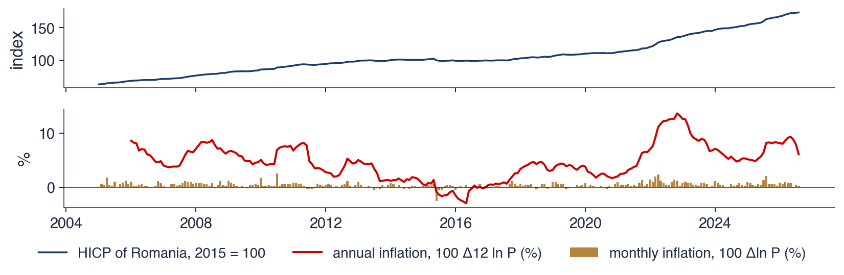
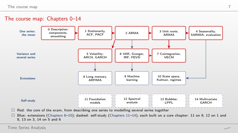

 TSA_ch15_box_jenkins