Bucharest University of Economic Studies IDA Institute Digital Assets Blockchain Research Center AI4EFin Artificial Intelligence for Energy Finance Romanian Academy, Institute for Economic Forecasting MSCA Digital Finance
The chapter asks whether tomorrow's risk can be forecast when tomorrow's return cannot. Chapters 1 to 3 modelled the conditional mean of a series, with ARMA and ARIMA models. Here the object of the model is the conditional variance, and the mean plays a secondary role.
The route has four stages. The first documents the stylised facts of returns and the tests for ARCH effects. The second defines the conditional variance and builds the ARCH and GARCH models. The third estimates them by maximum likelihood, with Student-t innovations and with an ARMA model for the mean. The fourth adds asymmetry, diagnostics, variance forecasts and their evaluation, and a one-day VaR 1%. Seminar 5 precedes this lecture and introduces the same data.
In brief
Question: if tomorrow's return cannot be predicted, can tomorrow's risk be predicted?
Chapters 1–3 modelled the conditional mean of a series; this chapter models its conditional variance
Route of the chapter
stylised facts of returns; the ACF of squared returns and the ARCH-LM test
conditional mean and conditional variance; ARCH(\(q\)) and GARCH(1,1); persistence, IGARCH and EWMA
estimation by maximum likelihood with the arch package; Student-t innovations; ARMA-GARCH models
asymmetry (GJR, EGARCH), diagnostics, variance forecasts and their evaluation, VaR 1%
Data: S&P 500, BET, EUR/RON (BNR reference rate) and Bitcoin, daily; Seminar 5 comes before this lecture
The outcomes follow the route of the chapter. The reader should be able to list the stylised facts and test for ARCH effects, to distinguish the conditional from the unconditional variance, and to explain why returns can be uncorrelated and still dependent. On the model side, the reader writes ARCH(\(q\)), GARCH(1,1) and ARMA-GARCH models and computes the persistence, the long-run variance and the half-life.
On the empirical side, the reader estimates GARCH models in Python by maximum likelihood, chooses the innovation distribution and checks the standardised residuals. The last outcomes concern asymmetry, measured with GJR-GARCH, EGARCH and the news impact curve, and forecasting: variance forecasts over several horizons, their evaluation with the QLIKE loss and a one-day VaR 1%.
In brief
List the stylised facts of financial returns and test for ARCH effects with the ACF of squared returns and the ARCH-LM test
Distinguish the conditional from the unconditional variance, and explain why returns can be uncorrelated yet dependent
Write ARCH(\(q\)), GARCH(1,1) and ARMA-GARCH models; compute the persistence, the long-run variance and the half-life
Estimate GARCH models by maximum likelihood in Python, choose the innovation distribution and check the standardised residuals
Measure asymmetry with GJR-GARCH, EGARCH and the news impact curve
Forecast the variance over several horizons, evaluate the forecasts with QLIKE and compute a one-day VaR 1%
The course textbook is Huang and Petukhina (2022), whose Chapter 6 covers financial time series and the ARCH and GARCH models. Tsay (2010), Chapter 3, gives a fuller treatment of volatility models with financial applications, and Franke, Härdle and Hafner (2019), Chapter 13, places them in the statistics of financial markets. The theory of maximum likelihood for heteroskedastic time series models is in Hamilton (1994), Chapter 21.
The computations use Python. The arch package estimates the ARCH-family models, and statsmodels provides the Ljung–Box and ARCH-LM tests. The Quantlets of the chapter reproduce every chart and table, and the lecture notebook runs in Google Colab.
Traditional econometric models assume a constant one-period forecast variance. To generalize this implausible assumption, a new class of stochastic processes called autoregressive conditional heteroscedastic (ARCH) processes are introduced in this paper.
The models of Chapters 1–3 describe the conditional mean of a series: the best forecast of tomorrow's value given the past. For daily returns of financial assets this forecast is almost useless, because the direction of tomorrow's move is close to unpredictable. The size of tomorrow's move is a different matter. Large moves arrive in clusters, and a day of turmoil makes another day of turmoil more likely. A model that assumes a constant variance, as white noise does, misses this structure entirely, even when it describes the mean well.
This chapter models the conditional variance. Engle (1982) made yesterday's squared shock part of today's variance, and Bollerslev (1986) added yesterday's variance, which gives the GARCH(1,1) model, still the benchmark of the field. The chapter applies these models to four daily series with very different behaviour: the S&P 500, the BET index of the Bucharest Stock Exchange, the EUR/RON reference rate of the National Bank of Romania (BNR) and Bitcoin. The data run to 18 September 2026.
The variance model changes several practical results. Forecast intervals widen in crises and narrow in calm periods. Risk measures such as the one-day VaR 1% follow the state of the market. The persistence of volatility can be measured in days, through the half-life of a variance shock. On the S&P 500, the GARCH(1,1) model with Student-t innovations gives a half-life of 131 trading days, and the one-day VaR 1% on 18 September 2026 is 1.75%.
Daily log returns in % of the S&P 500 and the BET (since 2000), the EUR/RON reference rate (since July 2005) and Bitcoin (since September 2014), to 18 September 2026; the shaded bands mark the global financial crisis (September 2008 – March 2009) and the COVID-19 crash (February – May 2020).
What you will be able to do
Test for ARCH effects with the ACF of squared returns, the Ljung–Box test on squares and the ARCH-LM test.
Derive the unconditional variance, the kurtosis, the persistence and the half-life of ARCH and GARCH models.
Estimate GARCH, GJR-GARCH, EGARCH and ARMA-GARCH models by maximum likelihood and choose the innovation distribution.
Interpret the standardised residuals, the news impact curve and a forecast comparison with QLIKE and the Diebold–Mariano test.
Compute multi-step variance forecasts and a one-day VaR 1% from a GARCH model.
SummaryKey ideas, formulas and self-assessment questions.
Stylised facts of financial returns
Stylised facts are empirical regularities that hold across markets, periods and sampling frequencies. For daily returns, three of them shape the whole chapter: heavy tails, almost no autocorrelation in the returns themselves, and strong, slowly decaying autocorrelation in their squares. The third fact is volatility clustering, and it is the reason for conditional variance models.
The section examines the four series of the chapter, first as time plots, then through summary statistics and autocorrelation functions, and finally through two formal tests for ARCH effects: the Ljung–Box test on squared residuals and the ARCH-LM test of Engle (1982).
Question for the room In which year was the daily standard deviation of the S&P 500 returns lowest?
Answer
In 2017: 0.42%, followed by 2006 (0.63%) and 2005 (0.65%). From September 2008 to March 2009 the standard deviation was 3.52%, 8.3 times larger, and in February–May 2020 3.70% (8.8 times). For the EUR/RON the calmest year was 2024 (0.025%) and the most agitated 2008 (0.72%): the BNR kept the leu almost fixed in 2020, when equities went through their largest storm.
The chart shows daily log returns in percent, \(r_t = 100(\ln P_t - \ln P_{t-1})\), where \(P_t\) is the closing price or exchange rate on day \(t\). Log returns add up over time, and multiplying by 100 puts them on a scale where a typical daily move is around 1. This scale also matters for estimation, as the section on maximum likelihood explains. The S&P 500 and the BET start in 2000, the EUR/RON reference rate in July 2005 and Bitcoin in September 2014; all four end on 18 September 2026.
The four panels have different vertical scales, so the eye should compare patterns rather than levels. In every panel the series looks like noise around zero whose amplitude changes over time. The shaded bands mark the global financial crisis, from September 2008 to March 2009, and the COVID-19 crash, from February to May 2020. In both episodes the equity indices show long stretches of large moves of both signs, while the years before and after are much quieter.
In brief
Daily log returns \(r_t = 100(\ln P_t - \ln P_{t-1})\), in %, to 18 September 2026: S&P 500 and BET since 2000, EUR/RON (BNR reference rate) since July 2005, Bitcoin since September 2014
Shaded: the global financial crisis (September 2008 – March 2009) and the COVID-19 crash (February – May 2020)
The common pattern is that calm years alternate with storms: large changes are followed by large changes, of either sign, and small changes by small changes. Mandelbrot (1963) described this behaviour in speculative prices; it is now called volatility clustering. Clustering concerns the size of the moves, not their direction, so it is invisible to the autocorrelation of the returns themselves.
The numbers show how large the swings are. The daily standard deviation of the S&P 500 was 0.42% in 2017, a calm year, 3.52% from September 2008 to March 2009, 8.3 times larger, and 3.70% from February to May 2020, 8.8 times larger. The EUR/RON rate behaves differently: its daily standard deviation was 0.78% in the 2008 crisis but only 0.10% in 2020, because the BNR kept the leu almost fixed during the pandemic. The volatility of a managed exchange rate reflects the policy of the central bank as much as the market.
A model with a constant variance, such as the white noise of Chapter 1, describes none of these series. It would assign the same probability to a 3% move in 2017 and in March 2020.
In brief
Calm years alternate with storms: large changes follow large changes, of either sign
S&P 500: daily standard deviation 0.42% in 2017, 3.52% from September 2008 to March 2009 (\(\times\)8.3) and 3.70% in February–May 2020 (\(\times\)8.8)
EUR/RON: 0.78% in the 2008 crisis, only 0.10% in 2020: the BNR kept the leu almost fixed
A model with a constant variance (white noise, Chapter 1) describes none of these series
The two photographs mark the two episodes shaded in the charts. On 15 September 2008 Lehman Brothers filed for bankruptcy, and the financial crisis entered its acute phase. In March 2020 the COVID-19 pandemic closed economies, and the Financial District of New York emptied.
Both episodes show the property that the GARCH model will capture with a single number: persistence. Calm did not return the day after the shock, but only after months. A large shock to volatility raises the variance for a long time, and the variance then returns slowly to its usual level. The half-life computed later in the chapter turns this observation into a measurable quantity.
The table summarises each series by its number of daily observations \(T\), its standard deviation (s.d., in % per day), skewness, kurtosis, the first-order autocorrelations of \(r_t\) and of \(r_t^2\), the Ljung–Box statistic \(Q(10)\) for the returns and for their squares, and the ARCH-LM statistic with 5 lags. Kurtosis is \(K = E[(r-\mu)^4]/\sigma^4\) and skewness \(E[(r-\mu)^3]/\sigma^3\); the Normal distribution has \(K = 3\) and skewness 0.
The first fact is heavy tails. Kurtosis ranges from 13.7 for the S&P 500 to 18.1 for the EUR/RON rate, far above 3. Extreme days are therefore much more frequent than the Normal distribution predicts. The equity indices and Bitcoin have negative skewness (−0.35, −0.65 and −0.70), so their large falls are more extreme than their large rises; the EUR/RON rate has positive skewness, 0.73: a positive return means a weaker leu, so its most extreme moves are depreciations.
The second fact is the contrast between levels and squares. The Ljung–Box statistic \(Q(10)\) is compared with the \(\chi^2(10)\) distribution, whose 5% critical value is 18.31. For the returns it is between 20 (Bitcoin) and 222 (EUR/RON), so some autocorrelation exists in the levels, but for the squares it is between 213 (Bitcoin) and 6133 (S&P 500), 11 to 64 times larger. The ARCH-LM statistic with 5 lags, compared with the 5% critical value 11.07 of the \(\chi^2(5)\) distribution, is between 115 and 1684. Every series rejects the hypothesis of no ARCH effects by a wide margin.
In brief
\(T\)
s.d.
skew.
kurt.
\(\hat\rho_1(r)\)
\(\hat\rho_1(r^2)\)
\(Q(10)\), \(r\)
\(Q(10)\), \(r^2\)
LM(5)
S&P 500
6 714
\(1.21\)
\(\ensuremath{-}0.35\)
\(13.7\)
\(\ensuremath{-}0.10\)
\(0.31\)
96
6133
1684
BET
6 670
\(1.40\)
\(\ensuremath{-}0.65\)
\(14.1\)
\(0.11\)
\(0.33\)
108
2440
982
EUR/RON
5 352
\(0.28\)
\(0.73\)
\(18.1\)
\(0.17\)
\(0.34\)
222
2420
871
Bitcoin
4 384
\(3.49\)
\(\ensuremath{-}0.70\)
\(15.0\)
\(\ensuremath{-}0.02\)
\(0.14\)
20
213
115
Heavy tails: kurtosis between 13.7 and 18.1, far above 3, the value of the Normal distribution
Little autocorrelation in \(r_t\), strong autocorrelation in \(r_t^2\): \(Q(10)\) of the squares is 11–64 times larger
\(Q(10)\): the statistic of Ljung and Box (1978) (Chapter 1), \(\chi^2(10)\), 5% value 18.31; LM(5): the ARCH-LM test (two slides ahead), \(\chi^2(5)\), 5% value 11.07
Question for the room Replace r² by |r|. How many of the 50 autocorrelations of |r| for the S&P 500 lie outside the band, and what is the autocorrelation at lag 50?
Answer
All 50 lie outside the band, and at lag 50 the autocorrelation is 0.127, against 0.053 for r²; at lag 1: 0.289 against 0.313. The absolute value is less dominated by a few extreme days than the square, so the memory of the size of returns shows even more clearly. The sign (r) stays almost unpredictable: 15 of 50 autocorrelations are outside the band, most of them small.
The chart plots the sample autocorrelation function (ACF) of \(r_t\) (blue bars) and of \(r_t^2\) (red bars) for lags 1 to 50, one panel per market. The shaded band \(\pm 1.96/\sqrt{T}\) is the approximate 95% band for the autocorrelations of an i.i.d. (independent and identically distributed) series: a bar outside the band is individually significant at 5%.
The blue bars stay almost entirely inside the band, apart from the first lag of the BET and the EUR/RON rate. The red bars are positive, large and decay slowly: for the S&P 500 they start above 0.3 and are still above the band after 50 trading days, about two and a half months. Bitcoin is the exception in degree but not in kind, with smaller red bars that still leave the band at several lags.
In brief
Sample ACF (autocorrelation function, Chapter 1) of \(r_t\) and of \(r_t^2\), lags 1–50, with the band \(\pm 1.96/\sqrt{T}\) of an i.i.d. (independent and identically distributed) series
The returns are close to white noise. Almost all their autocorrelations lie inside the band, so the direction of tomorrow's move is almost unpredictable from past returns. The BET is the visible exception, with \(\hat\rho_1 = 0.11\): in a thinner market prices adjust more slowly to news, which creates a small positive autocorrelation of the kind modelled in Chapter 2.
The squared returns tell another story. For the S&P 500 the autocorrelation of \(r_t^2\) is 0.31 at lag 1 and still 0.05 at lag 50, and all 50 lags lie outside the band. A large move today makes a large move tomorrow more likely, so the size of tomorrow's move is predictable. Bitcoin shows the same pattern more weakly, with \(\hat\rho_1(r_t^2) = 0.14\), because a few huge days dominate the squares and dilute the correlations.
Together the two ACFs show that uncorrelated is not the same as independent. A series can have zero autocorrelation at every lag and still be dependent, because a nonlinear function of it, here the square, is autocorrelated. Daily returns are close to white noise but not i.i.d., which is the distinction made in Chapter 1.
In brief
Returns: almost all autocorrelations inside the band (BET: \(\hat\rho_1 = 0.11\), a thin market; Chapter 2)
the direction of tomorrow's move is almost unpredictable
Squared returns: S&P 500 0.31 at lag 1 and still 0.05 at lag 50; 50 of 50 lags outside the band
the size of tomorrow's move is predictable: a large move today makes a large move tomorrow more likely
Uncorrelated is not the same as independent: \(r_t\) is close to white noise but not i.i.d. (Chapter 1)
Bitcoin: weaker but significant (\(\hat\rho_1(r_t^2) = 0.14\)): a few huge days dominate the squares
A series has ARCH effects when its conditional variance depends on the past. The name comes from the ARCH model of Section 3, but the tests do not require that model; they only ask whether past squared shocks predict current squared shocks. Both tests are applied to the residuals \(\hat\varepsilon_t\) of a model for the mean; for returns with a constant mean the residuals are simply \(r_t - \bar r\).
The first test is the Ljung–Box test applied to the squared residuals, as proposed by McLeod and Li (1983):
where \(\hat\rho_k(\hat\varepsilon^2)\) is the sample autocorrelation of the squared residuals at lag \(k\),\(m\) the number of lags and \(T\) the number of observations. Under the null hypothesis of no ARCH effects, \(Q(m)\) is approximately \(\chi^2(m)\). The statistic is the one of Ljung and Box (1978); only the series to which it is applied changes.
The second is the ARCH-LM test of Engle (1982), a Lagrange multiplier test computed from an auxiliary regression estimated by ordinary least squares (OLS):
Here \(q\) is the number of lagged squares, \(R^2\) the coefficient of determination of the regression and \(n\) the number of observations used in it. If past squares have no predictive power, \(R^2\) is close to zero and \(nR^2\) is small. The same two tests are run again on the standardised residuals after a volatility model has been fitted; then they check whether the model has removed the ARCH effects.
In brief
ARCH effects: the conditional variance depends on the past (the name comes from the ARCH model, Section 3)
Ljung–Box on squares (the test of McLeod and Li (1983)): \(Q(m) = T(T+2)\sum_{k=1}^{m}\hat\rho_k^2(\hat\varepsilon^2)/(T-k)\)
\(\hat\rho_k(\hat\varepsilon^2)\): the sample autocorrelation of the squared residuals at lag \(k\); \(m\): the number of lags; \(T\): the number of observations
\(\hat\varepsilon_t\): residuals of the mean model (for returns, \(r_t - \bar r\)); under \(H_0\) (no ARCH effects), \(Q(m) \sim \chi^2(m)\)
ARCH-LM testEngle (1982): LM (Lagrange multiplier) test from the auxiliary regression
\(\hat\varepsilon_t^2 = b_0 + b_1\hat\varepsilon_{t-1}^2 + \dots + b_q\hat\varepsilon_{t-q}^2 + u_t\), estimated by OLS (ordinary least squares)
\(b_0, \dots, b_q\): the coefficients; \(q\): the number of lagged squares; \(R^2\): the coefficient of determination of this regression
\(H_0\): \(b_1 = \dots = b_q = 0\); \(\mathrm{LM} = n R^2 \sim \chi^2(q)\), \(n\) = number of observations in the regression
Both tests are run on the residuals of the mean model, before and after fitting a volatility model
The example applies (5.1) to the BET. The mean model is an AR(1), the order chosen in Chapter 2, with estimated coefficient \(\hat\phi = 0.109\). Its residuals \(\hat\varepsilon_t\) are squared, and the squares are regressed on their own five lags, so \(q = 5\).
The estimated regression is \(\hat\varepsilon_t^2 = 0.862 + 0.276\,\hat\varepsilon_{t-1}^2 + 0.099\,\hat\varepsilon_{t-2}^2 + 0.088\,\hat\varepsilon_{t-3}^2 - 0.015\,\hat\varepsilon_{t-4}^2 + 0.102\,\hat\varepsilon_{t-5}^2\), with \(R^2 = 0.1526\) on \(n = 6\,664\) observations. The test statistic is \(\mathrm{LM} = nR^2 = 6\,664 \times 0.1526 = 1017\). The 5% critical value of the \(\chi^2(5)\) distribution is 11.07, so the hypothesis of no ARCH effects is rejected by a very wide margin: the variance of the BET depends on the last five squared shocks.
An \(R^2\) of 0.15 would be modest for a regression in levels, but squared returns are extremely noisy measures of the variance, so even a perfect variance model explains only a small part of their variation. In this context an \(R^2\) of 0.15 is a strong signal. The coefficient on the first lag, 0.276, is the largest, and the coefficients decline with the lag, the pattern that the ARCH and GARCH models describe.
In brief
Mean model: AR(1) for the BET returns (Chapter 2), \(\hat\phi = 0.109\); residuals \(\hat\varepsilon_t\); \(q = 5\)
Daily returns of the four markets share heavy tails, volatility clustering, little autocorrelation in the returns and strong autocorrelation in their squares. ARCH effects are detected with the Ljung–Box test on squared residuals and with the ARCH-LM test, \(\mathrm{LM} = nR^2 \sim \chi^2(q)\). All four series reject the null hypothesis of no ARCH effects by a wide margin.
In brief
Heavy tails, volatility clustering, little autocorrelation in \(r_t\), strong autocorrelation in \(r_t^2\)
The section has established what a model for daily returns must reproduce. The mean is almost unpredictable, but the variance changes over time and is predictable from the recent past: a large move today signals a high variance tomorrow. The tails are much heavier than those of the Normal distribution. On all four markets the tests for ARCH effects reject the constant-variance hypothesis by a margin of hundreds or thousands of units over the critical value, so the next step is a model in which the variance itself depends on the past.
Conditional mean and conditional variance
Before writing a volatility model, the chapter needs a precise language for "the variance given the past". This section defines the information set, the conditional mean and the conditional variance, and the decomposition \(r_t = \mu_t + \sigma_t z_t\) on which every model of the chapter rests. It then shows, with a two-state example and with the residuals of an ARMA model for the BET, why a correct model of the mean can still leave strong dependence in the squares.
Let \(\mathcal{F}_{t-1}\) denote the information available at the end of day \(t-1\), that is, all past values of the series. The conditional expectation \(E[X \mid \mathcal{F}_{t-1}]\) is the best forecast of a random variable \(X\), in the mean-squared-error sense, given that information, as in Chapter 2. Applied to the return, it defines the conditional mean \(\mu_t = E[r_t \mid \mathcal{F}_{t-1}]\). An ARMA model is a model for \(\mu_t\); for daily returns \(\mu_t\) is small and almost constant.
The conditional variance is the expected squared deviation from the conditional mean, given the past:
Its square root \(\sigma_t\) is the conditional volatility. It is known at the end of day \(t-1\) and changes from one day to the next. A series whose conditional variance is not constant is called conditionally heteroskedastic.
The unconditional variance \(\mathrm{Var}(r_t)\) is a different object: a single number for the whole sample, which ignores the information in the past. A stationary process can have a constant unconditional variance while its conditional variance moves every day. The stylised facts concern exactly this case.
In brief
\(\mathcal{F}_{t-1}\): the information available at the end of day \(t-1\) (all past values)
conditional expectation \(E[X \mid \mathcal{F}_{t-1}]\): the best forecast of \(X\) given the past (Chapter 2)
The innovations \(z_t\) are i.i.d. with mean 0 and variance 1; their distribution can be Normal, Student-t or another standardised law. The shock \(\varepsilon_t\) is the unpredictable part of the return. Both \(\mu_t\) and \(\sigma_t\) depend only on the past, so they are known at \(t-1\), while \(z_t\) is new on day \(t\).
Three consequences follow. First, \(E[\varepsilon_t \mid \mathcal{F}_{t-1}] = \sigma_t E[z_t] = 0\): the shocks form a martingale difference sequence, and a martingale difference with finite variance is uncorrelated, hence white noise. Second, \(\mathrm{Var}(\varepsilon_t \mid \mathcal{F}_{t-1}) = \sigma_t^2 E[z_t^2] = \sigma_t^2\), so the variance of tomorrow's shock is predictable. Third, the shocks are uncorrelated but not independent: when \(\sigma_t^2\) depends on \(\varepsilon_{t-1}^2\), the squares \(\varepsilon_t^2\) and \(\varepsilon_{t-1}^2\) are correlated.
The decomposition separates the two modelling tasks. An ARMA model, as in Chapter 2, describes \(\mu_t\); a GARCH model, the subject of this chapter, describes \(\sigma_t^2\). Estimated together, they form an ARMA-GARCH model.
In brief
Every model of this chapter: \(r_t = \mu_t + \varepsilon_t\), \(\varepsilon_t = \sigma_t z_t\)
\(z_t\): the innovations, i.i.d. with mean 0 and variance 1 (Normal, Student-t, …)
\(\varepsilon_t\): the shock; \(\mu_t\) and \(\sigma_t\) depend only on the past
Consequences
\(E[\varepsilon_t \mid \mathcal{F}_{t-1}] = \sigma_t E[z_t] = 0\): the shocks are a martingale difference, hence uncorrelated (white noise)
\(\mathrm{Var}(\varepsilon_t \mid \mathcal{F}_{t-1}) = \sigma_t^2\): the variance is predictable
the \(\varepsilon_t\) are uncorrelated but not independent: \(\varepsilon_t^2\) is correlated with \(\varepsilon_{t-1}^2\)
Two models, one for each moment: ARMA for \(\mu_t\) (Chapter 2), GARCH for \(\sigma_t^2\) (this chapter); together: ARMA-GARCH
Worked example: conditional and unconditional variance
Consider a market with calm days, on which \(\sigma_t^2 = 0.5\), and stormy days, on which \(\sigma_t^2 = 4.5\), each with probability 1/2, and with mean zero. The law of total variance splits the unconditional variance into the average conditional variance and the variance of the conditional mean:
Here the second term is zero, so \(\mathrm{Var}(r_t) = 0.5 \times 0.5 + 0.5 \times 4.5 = 2.50\), and the unconditional standard deviation is \(\sqrt{2.5} = 1.58\%\).
The unconditional figure is an average that describes no actual day. A calm day has \(\sigma_t = \sqrt{0.5} = 0.71\%\) and a stormy day \(\sigma_t = \sqrt{4.5} = 2.12\%\). The conditional variance tells which kind of day we are in; the unconditional variance does not. A risk manager using 1.58% would overstate the risk on calm days and understate it on stormy days.
The mixture has another consequence. With Normal \(z_t\), the kurtosis of \(r_t\) equals \(3E[\sigma_t^4]/(E[\sigma_t^2])^2\). Here \(E[\sigma_t^4] = 0.5 \times 0.25 + 0.5 \times 20.25 = 10.25\) and \((E[\sigma_t^2])^2 = 6.25\), so the kurtosis is \(3 \times 10.25/6.25 = 4.92\). A time-varying variance alone creates heavy tails, even when every day's distribution is Normal. Part of the kurtosis in the table of the previous section is explained this way.
In brief
A market has calm days (\(\sigma_t^2 = 0.5\)) and stormy days (\(\sigma_t^2 = 4.5\)), each with probability \(1/2\); the mean is 0
law of total variance: \(\mathrm{Var}(r_t) = E[\mathrm{Var}(r_t \mid \mathcal{F}_{t-1})] + \mathrm{Var}(E[r_t \mid \mathcal{F}_{t-1}])\)
step by step: \(0.5 \times 0.5 + 0.5 \times 4.5 + 0 = 2.50\); unconditional standard deviation \(1.58\%\)
The unconditional variance is an average; the conditional variance tells which day we are in
a calm day: \(\sigma_t = 0.71\%\); a stormy day: \(\sigma_t = 2.12\%\); the average \(1.58\%\) fits neither
With Normal \(z_t\), the mixture has kurtosis \(3E[\sigma_t^4]/(E[\sigma_t^2])^2 = 4.92\): a time-varying variance creates heavy tails
Question for the room Raise the AR order of the mean from 1 to 5. Do the ARCH effects of the residuals disappear?
Answer
No. Q(10) of the residuals falls from 29.7 to 15.4 (p = 0.009), but Q(10) of the squares rises from 2496 to 2562, and ARCH-LM(5) stays around 1020 (for AR(1): n R² = 6664 × 0.1526 = 1017). A richer model for the mean removes the autocorrelation of the level, not that of the squares: the conditional variance needs a model of its own. On the right, the same residuals divided by the GARCH(1,1) volatility lose their ARCH effects for every p: Q(10) of ẑ² stays between 7.0 and 8.3 (p > 0.6).
The chart compares two models for the BET. On the left, an AR(1) model for the mean with a constant variance; the order \(p = 1\) was chosen by the Bayesian information criterion (BIC) among AR(0) to AR(5). The blue bars are the autocorrelations of its residuals and the red bars those of the squared residuals. On the right, the same AR(1) mean with a GARCH(1,1) variance and Student-t innovations, the model of Section 6; the bars are the autocorrelations of the standardised residuals \(\hat z_t = \hat\varepsilon_t/\hat\sigma_t\) and of their squares.
The two panels share the vertical axis. On the left the red bars rise far above the shaded band at every lag up to 30; on the right both kinds of bars stay close to zero. The comparison is the empirical counterpart of the decomposition (5.2): the mean model handles the blue bars, and only a variance model handles the red ones.
In brief
BET: left, an AR(1) for the mean (order chosen by BIC among AR(0)–AR(5): \(p = 1\)), constant variance; right, the same AR(1) with a GARCH(1,1)-t variance (Section 6)
On the left, the residuals of the AR(1) look almost like white noise, so the Box–Jenkins check of Chapter 2, which looks only at the residuals, would nearly be passed. Their squares, however, have first-order autocorrelation 0.34 and a Ljung–Box statistic \(Q(10) = 2496\), far above the 5% critical value of 18.31. The AR(1) has captured the mean but left strong ARCH effects.
On the right, after division by the GARCH volatility \(\hat\sigma_t\), the squares are clean: their first-order autocorrelation is 0.018, \(Q(10)\) is 7.2 with p-value 0.705, and the ARCH-LM statistic is 4.8 with p-value 0.446. A little autocorrelation remains in the levels, with \(Q(10) = 28.6\) for \(\hat z_t\), which suggests that the BET mean has more structure than an AR(1) can capture.
The lesson is methodological. A model check must look at both \(\hat\varepsilon_t\) and \(\hat\varepsilon_t^2\). A white-noise test on the residuals alone is blind to the variance, and a model that passes it can still produce badly wrong forecast intervals.
In brief
Left: the residuals look almost like white noise, the Box–Jenkins check of Chapter 2 would be nearly passed
but their squares: \(\hat\rho_1 = 0.34\), \(Q(10) = 2496\): strong ARCH effects
Right: after dividing by \(\hat\sigma_t\), the squares are clean: \(\hat\rho_1 = 0.018\), \(Q(10) = 7.2\) (p = 0.705), ARCH-LM 4.8 (p = 0.446)
some autocorrelation in the level remains (\(Q(10) = 28.6\)): the BET mean has more structure than an AR(1)
Lesson: check both \(\hat\varepsilon_t\) and \(\hat\varepsilon_t^2\); a white-noise check on \(\hat\varepsilon_t\) alone misses the variance
The decomposition \(r_t = \mu_t + \sigma_t z_t\) gives one model for each moment: an ARMA model for \(\mu_t\) and a volatility model for \(\sigma_t^2\). The shocks are uncorrelated but dependent through their squares. The unconditional variance is the average of the conditional variances, and the mixture of variances produces heavy tails.
In brief
\(r_t = \mu_t + \sigma_t z_t\): \(\mu_t\) from an ARMA model, \(\sigma_t^2\) from a volatility model
Shocks are uncorrelated but dependent through their squares
Unconditional variance = average of the conditional variances; the mixture has heavy tails
Section summary
The conditional variance is the variance of tomorrow's return given today's information; the unconditional variance is its long-run average. Shocks built as \(\varepsilon_t = \sigma_t z_t\) are a martingale difference, hence white noise, yet their squares are correlated whenever \(\sigma_t\) depends on the past. On the BET, an AR(1) mean model passes a white-noise check on its residuals while their squares have a Ljung–Box statistic of 2496; adding a GARCH(1,1) variance brings that statistic down to 7.2. The next section builds the first model for \(\sigma_t^2\).
The ARCH model
The first model for the conditional variance makes today's variance a linear function of yesterday's squared shock. This section presents the ARCH(1) model of Engle (1982), derives its unconditional variance and kurtosis, compares simulated ARCH paths with i.i.d. and GARCH paths, and shows on the S&P 500 why ARCH needs many lags to fit real data.
Engle (1982) introduced the autoregressive conditional heteroskedasticity (ARCH) model: today's variance depends on yesterday's squared shocks. The first application was not a financial market but the variance of inflation in the United Kingdom, where the uncertainty of the forecast itself was the object of interest. The model was soon adopted in finance, where volatility clustering is the dominant feature of the data.
In 2003 Engle received the Nobel Prize in Economic Sciences "for methods of analyzing economic time series with time-varying volatility (ARCH)". He shared it with Clive Granger, whose work on spurious regression appears in Chapter 3 and on cointegration in Chapter 7. The Nobel lecture, Engle (2004), surveys the use of ARCH models in risk management.
The constant \(\omega\) is the minimum level of the variance, reached after a zero shock. The coefficient \(\alpha\) measures how strongly the variance reacts to yesterday's squared shock. The restrictions \(\omega > 0\) and \(\alpha \ge 0\) guarantee a positive variance. Because only the square of the shock enters, a large shock of either sign raises today's variance.
The word "autoregressive" refers to the squared shocks. Write \(\varepsilon_t^2 = \sigma_t^2 + v_t\), with \(v_t = \sigma_t^2(z_t^2 - 1)\). Since \(E[z_t^2] = 1\),\(E[v_t \mid \mathcal{F}_{t-1}] = 0\), so \(v_t\) is a martingale difference. Substituting the variance equation gives
an AR(1) model for \(\varepsilon_t^2\), as in Chapter 2, with white-noise errors \(v_t\).
The AR(1) form gives the autocorrelations of the squares directly: when the fourth moment exists, \(\rho_k(\varepsilon_t^2) = \alpha^k\). ARCH(1) therefore produces clustering, but the correlation of the squares decays geometrically at rate \(\alpha\). For moderate values of \(\alpha\) this decay is much faster than the slow decay seen in real squared returns.
The shocks of an ARCH(1) have mean zero and are uncorrelated at every lag \(k \ne 0\), so they are white noise. When \(\alpha < 1\) the process is stationary, and its unconditional variance follows from taking expectations in the variance equation: \(\bar\sigma^2 = E[\varepsilon_t^2] = \omega + \alpha\bar\sigma^2\), so
\[\bar\sigma^2 = \frac{\omega}{1-\alpha}.\]
With Normal innovations and \(3\alpha^2 < 1\), the kurtosis of the shocks is
\[K = 3\,\frac{1-\alpha^2}{1-3\alpha^2} > 3.\]
The innovations are Normal, yet the shocks have heavy tails, for the same reason as in the two-state example: a mixture of Normal distributions with different variances. If \(\alpha \ge 1/\sqrt{3} = 0.577\), the fourth moment is infinite, although the variance is still finite as long as \(\alpha < 1\).
In the worked example \(\omega = 0.5\) and \(\alpha = 0.5\). The unconditional variance is \(0.5/0.5 = 1.00\), and the kurtosis is \(3 \times 0.75/0.25 = 9.0\). After a shock \(\varepsilon_{t-1} = 2\), two unconditional standard deviations, the next variance is \(\sigma_t^2 = 0.5 + 0.5 \times 4 = 2.50\), so \(\sigma_t = 1.58\): the variance more than doubles relative to its average level of 1.
In brief
\(E[\varepsilon_t] = 0\) and \(\mathrm{Cov}(\varepsilon_t, \varepsilon_{t-k}) = 0\) for \(k \ne 0\): white noise
Unconditional variance (stationary if \(\alpha < 1\)): take expectations in \(\sigma_t^2 = \omega + \alpha\varepsilon_{t-1}^2\)
Question for the room Move α of ARCH(1) to 0.7 (ω = 0.3). What are the theoretical and the sample kurtosis?
Answer
In theory the fourth moment does not exist (3α² = 1.47 ≥ 1, the threshold is α = 1/√3 = 0.577), so the kurtosis is infinite. The kurtosis of the 1000 simulated values is 11.24, and 34.9 at α = 0.9: a finite sample always has a finite kurtosis, so the sample value cannot show that the moment does not exist. At α = 0.5 theory gives 9.0 and the sample 4.91: the fourth moment converges slowly.
The chart shows three simulated series of 1000 values, all with unconditional variance 1. The top panel is i.i.d. Normal noise. The middle panel is an ARCH(1) with \(\omega = \alpha = 0.5\), the model of the previous frame. The bottom panel is a GARCH(1,1) with \(\omega = 0.02\),\(\alpha = 0.10\) and \(\beta = 0.88\), the model of the next section. Since all three have the same variance, differences in appearance come only from the dependence structure.
The ARCH(1) path shows isolated spikes: a large value is followed by a few agitated days, and the effect fades quickly because the memory is one day. The GARCH(1,1) path shows long calm stretches and long agitated stretches, which is what the return series of the four markets look like. The sample kurtosis is 3.12 for the i.i.d. series, 4.91 for the ARCH and 3.74 for the GARCH series, against theoretical values of 3, 9.0 and 6.06. The gap between sample and theory shows that the fourth moment of heavy-tailed processes converges slowly: 1000 observations are not enough to estimate it precisely.
In brief
Three series of 1000 values with unconditional variance 1: i.i.d. Normal; ARCH(1) with \(\omega = \alpha = 0.5\); GARCH(1,1) with \(\omega = 0.02\), \(\alpha = 0.10\), \(\beta = 0.88\) (next section)
Sample kurtosis: i.i.d. \(3.12\), ARCH \(4.91\), GARCH \(3.74\) (theory: 3, \(9.0\), \(6.06\)): the fourth moment converges slowly
Interpretation: ARCH(1) gives isolated spikes; GARCH(1,1) gives long calm and long agitated periods, as in real returns
The ARCH(\(q\)) model lets the variance depend on \(q\) past squared shocks: \(\sigma_t^2 = \omega + \alpha_1\varepsilon_{t-1}^2 + \dots + \alpha_q\varepsilon_{t-q}^2\), with \(\alpha_i \ge 0\). It is stationary if \(\sum_i \alpha_i < 1\), with unconditional variance \(\omega/(1 - \sum_i\alpha_i)\). Its weakness is structural: a shock affects the variance for exactly \(q\) days and then disappears from the equation, whereas real volatility clustering lasts for months.
The table fits ARCH(1), ARCH(5), ARCH(10) and GARCH(1,1) to the S&P 500 with Normal innovations. Each row gives the number of parameters \(k\), the maximised log-likelihood \(\ell\), the Akaike and Bayesian information criteria, \(\mathrm{AIC} = -2\ell + 2k\) and \(\mathrm{BIC} = -2\ell + k\ln T\)(Akaike, 1974; Schwarz, 1978), and the persistence: the sum of the \(\alpha_i\) for ARCH, \(\alpha + \beta\) for GARCH. Smaller criteria are better, and BIC penalises extra parameters more heavily than AIC.
The log-likelihood rises from −10305.5 for ARCH(1) to −9340.5 for ARCH(5) and −9227.6 for ARCH(10), so additional lags keep improving the fit. Yet GARCH(1,1), with 4 parameters, reaches −9218.0, higher than ARCH(10) with 12 parameters, and has the smallest AIC (18444.0) and BIC (18471.2). The persistence rises with the number of lags, from 0.394 to 0.849, and GARCH reaches 0.980. A long ARCH is trying to approximate a slowly decaying memory, which GARCH provides with one additional parameter.
ARCH models the variance as an autoregression of squared shocks, \(\sigma_t^2 = \omega + \sum_i\alpha_i\varepsilon_{t-i}^2\). Its unconditional variance is \(\omega/(1 - \sum\alpha_i)\), and its kurtosis exceeds 3 even with Normal innovations. Real clustering needs many lags, which GARCH replaces with a single extra parameter.
In brief
\(\sigma_t^2 = \omega + \sum_i\alpha_i\varepsilon_{t-i}^2\): an AR model for the squared shocks
Unconditional variance \(\omega/(1 - \sum\alpha_i)\); kurtosis above 3 even with Normal innovations
Real clustering needs many lags: GARCH replaces them with one extra parameter
Section summary
ARCH captures the core idea of the chapter: yesterday's squared shock predicts today's variance, and this alone produces uncorrelated returns with correlated squares and heavy tails. The memory of ARCH(\(q\)) is cut off after \(q\) days, however, so on the S&P 500 even ten lags fit worse than GARCH(1,1) with four parameters. The next section adds yesterday's variance to the equation and obtains a memory that decays slowly.
The GARCH(1,1) model
GARCH(1,1) adds one term to ARCH(1), yesterday's conditional variance, and thereby turns a one-day memory into a geometrically decaying memory of all past shocks. This section defines the model, writes it as an ARMA(1,1) for the squared shocks, derives the long-run variance, the kurtosis and the half-life of a shock, and works through a one-step update. It then treats the boundary case \(\alpha + \beta = 1\), the IGARCH model, and its relation to the EWMA estimator used in industry, and compares GARCH, EWMA and a rolling window during the COVID-19 crash.
Bollerslev (1986), then a doctoral student of Engle at the University of California, San Diego, proposed adding yesterday's variance to the ARCH equation. The resulting generalised ARCH (GARCH) model replaces a long ARCH(\(q\)) with a few parameters. A year later, Bollerslev (1987) combined GARCH with Student-t innovations for speculative prices and returns, the specification used for most estimates in this chapter.
GARCH(1,1) remains the benchmark. Hansen and Lunde (2005) compared 330 volatility models out of sample and found GARCH(1,1) hard to beat on exchange rates; their study is the case study of Section 9.
In brief
Bollerslev (1986), a doctoral student of Engle at the University of California, San Diego: add yesterday's variance to the equation
GARCH (generalised ARCH): a few parameters replace a long ARCH(\(q\))
The general GARCH(\(p\),\(q\)) adds more lags of both kinds, but in practice the (1,1) specification is almost always enough for daily returns. The parameters have a direct reading. The coefficient \(\alpha\) is the reaction of the variance to yesterday's news, the squared shock. The coefficient \(\beta\) is the memory of the variance, the weight on yesterday's level. Their sum \(\alpha + \beta\) is the persistence, and \(\omega\) sets, together with the persistence, the long-run level.
Substituting the equation into itself repeatedly gives
GARCH(1,1) is therefore an ARCH(\(\infty\)) with geometrically declining weights \(\alpha\beta^j\). All past shocks matter, and the weights decay at rate \(\beta\), slowly when \(\beta\) is close to 1. This is how three parameters in the variance equation reproduce the slow decay of the ACF of squared returns.
GARCH(\(p\),\(q\)) adds more lags of both kinds; in practice (1,1) is almost always enough
Reading the parameters
\(\alpha\): the reaction to yesterday's news; \(\beta\): the memory of the variance
\(\alpha + \beta\): the persistence; \(\omega\) sets the long-run level
By recursion: an ARCH(\(\infty\)) with geometric weights
\(\sigma_t^2 = \dfrac{\omega}{1 - \beta} + \alpha\sum_{j=0}^{\infty}\beta^j\,\varepsilon_{t-1-j}^2\): all past shocks matter, with weights that decay like \(\beta^j\)
As for ARCH, write \(\varepsilon_t^2 = \sigma_t^2 + v_t\), with \(v_t\) a martingale difference, and substitute \(\sigma_t^2 = \varepsilon_t^2 - v_t\) and \(\sigma_{t-1}^2 = \varepsilon_{t-1}^2 - v_{t-1}\) into (5.4):
This is an ARMA(1,1) model for \(\varepsilon_t^2\), as in Chapter 2, with autoregressive coefficient \(\alpha + \beta\) and moving-average coefficient \(-\beta\).
The ARMA form transfers the results of Chapter 2. The process is covariance stationary if \(\alpha + \beta < 1\), that is, if the AR root lies outside the unit circle. The ACF of \(\varepsilon_t^2\) decays like \((\alpha + \beta)^k\), slowly when the persistence is close to 1, which matches the ACF of real squared returns. In principle the model could be identified from the ACF and the partial autocorrelation function (PACF) of \(\varepsilon_t^2\), but the errors \(v_t\) are strongly heteroskedastic and heavy-tailed, so in practice GARCH models are estimated by maximum likelihood, the subject of Section 5.
In brief
As for ARCH, write \(\varepsilon_t^2 = \sigma_t^2 + v_t\) and substitute \(\sigma_t^2 = \varepsilon_t^2 - v_t\) in the equation
an ARMA(1,1) (Chapter 2) with AR coefficient \(\alpha + \beta\) and MA coefficient \(-\beta\)
Consequences
covariance stationary if \(\alpha + \beta < 1\) (the AR root outside the unit circle)
the ACF of \(\varepsilon_t^2\) decays like \((\alpha + \beta)^k\): slow when the persistence is close to 1, as in the ACF of real squared returns
identification by the ACF and the PACF (partial autocorrelation function) of \(\varepsilon_t^2\) is possible in principle, but in practice we use maximum likelihood (Section 5)
Long-run variance, kurtosis, persistence and half-life
When \(\alpha + \beta < 1\), taking expectations in (5.4) gives the long-run, or unconditional, variance
\[\bar\sigma^2 = \frac{\omega}{1-\alpha-\beta}.\]
For daily returns it is reported as an annualised volatility, \(\sqrt{252\,\bar\sigma^2}\), with 252 trading days per year. With Normal innovations, the kurtosis is \(K = 3\,[1-(\alpha+\beta)^2]/[1-(\alpha+\beta)^2-2\alpha^2]\), which exceeds 3; for \(\alpha = 0.10\) and \(\beta = 0.88\) it equals 6.06.
The persistence governs how fast the variance returns to \(\bar\sigma^2\). The forecast derived in Section 9 shows that a deviation from the long-run variance shrinks by the factor \(\alpha + \beta\) each day: \(E_t[\sigma_{t+h}^2] - \bar\sigma^2 = (\alpha+\beta)^{h-1}(\sigma_{t+1}^2 - \bar\sigma^2)\), where \(E_t\) is the expectation given the information of day \(t\) and \(\sigma_{t+1}^2\) is tomorrow's variance, already known at \(t\). The half-life is the number of days after which half of a variance shock is gone:
\[h_{1/2} = \frac{\ln 0.5}{\ln(\alpha+\beta)}.\]
(5.6)
The half-life is very sensitive to the persistence near 1. With \(\alpha + \beta = 0.90\) it is 6.6 days, with 0.98 it is 34.3 days, and with 0.99 it is 69.0 days. A change of 0.01 in the persistence doubles the duration of a shock, which is why the persistence estimates of the four markets in Section 6 translate into very different half-lives.
In brief
Long-run (unconditional) variance: \(\bar\sigma^2 = \omega/(1 - \alpha - \beta)\); annualised volatility \(\sqrt{252\,\bar\sigma^2}\) for 252 trading days
A deviation from \(\bar\sigma^2\) shrinks by the factor \(\alpha + \beta\) each day (Section 9): \(E_t[\sigma_{t+h}^2] - \bar\sigma^2 = (\alpha + \beta)^{h-1}(\sigma_{t+1}^2 - \bar\sigma^2)\)
\(E_t[\cdot]\): the expectation given the information of day \(t\); \(\sigma_{t+1}^2\): tomorrow's variance, already known at \(t\)
half-life: the number of days after which half of a variance shock is gone, \(h_{1/2} = \ln 0.5/\ln(\alpha + \beta)\)
\(\alpha + \beta = 0.90\): 6.6 days; \(0.98\): 34.3 days; \(0.99\): 69.0 days: small changes near 1 matter a lot
Take daily returns in percent with \(\omega = 0.02\),\(\alpha = 0.10\),\(\beta = 0.88\) and mean \(\mu = 0\), the parameters of the simulated GARCH path. The persistence is \(\alpha + \beta = 0.98\), the long-run variance is \(\bar\sigma^2 = 0.02/(1-0.98) = 1.00\), and the annualised long-run volatility is \(\sqrt{252 \times 1.00} = 15.9\%\). From (5.6) the half-life is \(\ln 0.5/\ln 0.98 = 34.3\) days.
Suppose today's conditional variance is \(\sigma_t^2 = 1.2\), slightly above the long-run level, and today's return is \(r_t = -3\%\), so \(\varepsilon_t^2 = 9\). Tomorrow's variance is \(\sigma_{t+1}^2 = 0.02 + 0.10 \times 9 + 0.88 \times 1.2 = 1.976\), and tomorrow's volatility is \(\sigma_{t+1} = 1.41\%\). The three terms show the roles of the parameters: the constant contributes 0.02, the news term 0.90 and the memory term 1.056.
A single 3% fall has raised the variance from 1.2 to almost 2. In the following days, without new large shocks, the excess over the long-run level of 1.00 shrinks by the factor 0.98 per day, so half of it is gone after about 34 trading days.
The boundary case \(\alpha + \beta = 1\) is the integrated GARCH (IGARCH) model of Engle and Bollerslev (1986). In the ARMA(1,1) form (5.5) the AR coefficient equals 1, so \(\varepsilon_t^2\) has a unit root, as in Chapter 3. Shocks to the variance never die out: the forecast of the variance does not return to any long-run level, the half-life is infinite and the unconditional variance is not finite.
The exponentially weighted moving average (EWMA) of the RiskMetrics methodology (J.P. Morgan/Reuters, 1996) is
The parameter \(\lambda\) is the weight of yesterday's variance and \(1 - \lambda\) the weight of yesterday's squared return. EWMA is simple exponential smoothing, from Chapter 0, applied to \(r_t^2\) with smoothing constant \(1 - \lambda\). It is also an IGARCH with \(\omega = 0\),\(\alpha = 1 - \lambda\) and \(\beta = \lambda\). RiskMetrics uses \(\lambda = 0.94\) for daily data, which gives the weights a half-life of \(\ln 0.5/\ln 0.94 = 11.2\) days.
The question on the slide makes the difference concrete. Right after a crash, an analyst forecasts the volatility one year ahead with EWMA. Because EWMA has no long-run level, its forecast for every future horizon equals today's crisis level, so the one-year forecast stays at the crisis level. A stationary GARCH lets the forecast decay towards the long-run level at the rate \(\alpha + \beta\). The two estimators can give similar day-to-day volatilities and very different long-horizon forecasts.
\(\lambda \in (0, 1)\): the weight of yesterday's variance; \(1 - \lambda\): the weight of yesterday's squared return
simple exponential smoothing (Chapter 0) applied to \(r_t^2\), with smoothing constant \(1 - \lambda\)
an IGARCH with \(\omega = 0\), \(\alpha = 1 - \lambda\), \(\beta = \lambda\); RiskMetrics uses \(\lambda = 0.94\) for daily data (half-life of the weights 11.2 days)
Question for the room: right after a crash, an analyst forecasts the volatility one year ahead with EWMA. What goes wrong?
Answer: EWMA keeps today's crisis level for the whole year; GARCH lets it decay towards the long-run level
Question for the room Raise λ to 0.97. Is the EWMA peak of March 2020 higher or lower than 85%?
Answer
Lower: 67%, on 27 March 2020, against 85% on 25 March for λ = 0.94. With a larger λ the weight of yesterday’s return, 1 − λ, falls from 0.06 to 0.03, and the half-life of the weights rises from 11.2 to 22.8 days: the estimate reacts more slowly and comes down more slowly (37% on 30 June 2020, against 30%). With λ = 0.90 the peak is 103%, close to that of GARCH (111%), whose α = 0.123 is larger than 1 − λ = 0.06.
The chart compares three estimates of the annualised volatility of the S&P 500 from late 2019 to early 2021. The solid blue line is the GARCH(1,1)-t volatility, estimated on all data. The dashed red line is EWMA with \(\lambda = 0.94\). The green line is the standard deviation of the last 63 trading days, about three months, a moving average of the kind seen in Chapter 0.
All three are low and close together before February 2020. In March 2020 the GARCH line rises first and highest, EWMA follows slightly below, and the rolling window rises slowly to a plateau. The most instructive part of the chart is the period from April to June 2020, when the three lines separate and then come back together.
In brief
S&P 500, annualised volatility: GARCH(1,1)-t estimated on all data, EWMA with \(\lambda = 0.94\), and the standard deviation of the last 63 days (Chapter 0: a moving average)
The peaks differ in level and date. GARCH peaks at 111% on 17 March 2020, EWMA at 85% on 25 March 2020 and the 63-day window at 63% on 20 May 2020, two months after the crash. The rolling window gives equal weight to all 63 days, so it reacts late; when the crash days leave the window, it falls abruptly although nothing happened on that day in the market. This drop is the "ghost" of the crash: an artefact of the window length, not a change in risk.
By 30 June 2020 the three estimates are close again: GARCH 28%, EWMA 30% and the window 32%. GARCH reacts fastest because its \(\alpha\), 0.123 for the S&P 500, is larger than the EWMA weight \(1 - \lambda = 0.06\). It also decays fastest, because a stationary GARCH reverts to its long-run level, while EWMA only forgets old observations. EWMA lies between GARCH and the rolling window on both counts.
In brief
Peaks: GARCH 111% (17 March 2020), EWMA 85% (25 March 2020), 63-day window 63% (20 May 2020)
The rolling window reacts late and falls abruptly when the crash leaves the window (the “ghost” of the crash)
on 30 June 2020: GARCH 28%, EWMA 30%, window 32%
GARCH reacts fastest (\(\alpha\) larger than \(1 - \lambda\)) and decays fastest (mean reversion); EWMA lies in between
GARCH(1,1), \(\sigma_t^2 = \omega + \alpha\varepsilon_{t-1}^2 + \beta\sigma_{t-1}^2\), combines a reaction \(\alpha\) to yesterday's news with a memory \(\beta\) of yesterday's variance, and is an ARMA(1,1) for \(\varepsilon_t^2\). When \(\alpha + \beta < 1\), the long-run variance is \(\omega/(1-\alpha-\beta)\) and the half-life \(\ln 0.5/\ln(\alpha+\beta)\). When \(\alpha + \beta = 1\), the model is IGARCH, and EWMA is an IGARCH without \(\omega\).
In brief
\(\sigma_t^2 = \omega + \alpha\varepsilon_{t-1}^2 + \beta\sigma_{t-1}^2\): reaction \(\alpha\), memory \(\beta\); an ARMA(1,1) for \(\varepsilon_t^2\)
\(\alpha + \beta = 1\): IGARCH; EWMA is an IGARCH without \(\omega\)
Section summary
GARCH(1,1) describes volatility with three numbers: how much the variance reacts to news, how much it remembers, and the level to which it returns. Its ARMA(1,1) form explains the slow decay of the autocorrelations of squared returns, and the persistence \(\alpha + \beta\) converts directly into a half-life: 34.3 days for a persistence of 0.98. The boundary case \(\alpha + \beta = 1\) links GARCH to the EWMA of RiskMetrics, which never returns to a long-run level. During the COVID-19 crash, GARCH reacted fastest and faded fastest, while a 63-day rolling window peaked two months late. The parameters still have to be estimated, which is the subject of the next section.
Estimation by maximum likelihood
The variance \(\sigma_t^2\) is not observed, so GARCH parameters cannot be estimated by regressing anything on anything. They are estimated by maximum likelihood, building the likelihood from the conditional densities implied by (5.2). This section writes the likelihood, shows its shape on simulated ARCH and GARCH data, estimates the S&P 500 model both step by step and with the arch package, explains quasi-maximum likelihood and robust standard errors, and replaces the Normal distribution of the innovations with the Student-t and skewed-t distributions.
Returns are dependent through their variance, so their joint density is not the product of the marginal densities. It is a product of conditional densities:
With Normal innovations and a constant mean \(\mu\), each conditional density is Normal, \(r_t \mid \mathcal{F}_{t-1} \sim N(\mu, \sigma_t^2)\). Ignoring the first observation gives the conditional log-likelihood of the parameter vector \(\theta = (\mu, \omega, \alpha, \beta)\):
The variance \(\sigma_t^2(\theta)\) is computed recursively from the GARCH equation, starting from a value \(\sigma_1^2\) such as the sample variance. Each term of the sum rewards a small variance through \(\ln\sigma_t^2\) and penalises a variance that is too small for the observed squared deviation through \((r_t-\mu)^2/\sigma_t^2\). The likelihood is maximised by a variance path that follows the squared returns without overreacting to them.
The maximum likelihood estimator (MLE) is \(\hat\theta = \arg\max_\theta \ell(\theta)\), subject to \(\omega > 0\),\(\alpha, \beta \ge 0\) and \(\alpha + \beta < 1\). There is no closed form, so a numerical optimiser searches for the maximum. OLS is not possible, because the dependent variable of the variance equation, \(\sigma_t^2\), is not observed.
In brief
The returns are dependent, so the joint density is a product of conditional densities
\(f(r_1, \dots, r_T) = f(r_1)\prod_{t=2}^{T} f(r_t \mid \mathcal{F}_{t-1})\), with \(r_t \mid \mathcal{F}_{t-1} \sim N(\mu, \sigma_t^2)\) for Normal innovations
Question for the room Move the second sample to n = 5000. What does the standard error of α̂ become?
Answer
0.015 (α̂ = 0.516), against 0.035 for n = 1000: 2.3 times smaller, close to √5 = 2.24. The standard error falls with √n, because the log-likelihood is a sum of n terms and its curvature at the maximum grows in proportion to n.
The chart shows the log-likelihood of an ARCH(1) model as a function of \(\alpha\) for data simulated with \(\omega = \alpha = 0.5\). To obtain a curve in one parameter, \(\omega\) is tied to \(\alpha\) through \(\omega = 1 - \alpha\), which keeps the unconditional variance at 1. Each curve is shifted so that its maximum is zero, and the vertical lines mark the location of each maximum and the true value \(\alpha = 0.5\).
With \(n = 100\) observations the curve (blue) is flat: the maximum is at \(\hat\alpha = 0.432\), and a wide range of values has a log-likelihood within a few units of it. The standard error is 0.127. With \(n = 1000\) (red) the curve is much sharper, the maximum is at \(\hat\alpha = 0.491\), close to the truth, and the standard error falls to 0.035.
The standard error of the MLE comes from the curvature of the log-likelihood at its maximum: the inverse of the negative second derivative (the Hessian) estimates the variance of \(\hat\theta\). A sharp peak means a precise estimate. Ten times more data make the curvature about ten times larger and the standard error about \(\sqrt{10}\) times smaller, here from 0.127 to 0.035.
In brief
Simulated ARCH(1) with \(\omega = \alpha = 0.5\); \(\ell(\alpha)\) with \(\omega = 1 - \alpha\); each curve minus its maximum
Question for the room With n = 1000 in the right panel, where is the maximum on the grid?
Answer
At (0.045, 0.90): α is still underestimated and β overestimated, along the same ridge on which α + β changes little. With n = 1500 the maximum is at (0.075, 0.82), with n = 3000 at (0.10, 0.81), with n = 5000 at (0.10, 0.82). α and β trade off: different pairs with the same persistence give almost the same likelihood, which is why GARCH needs long samples.
The chart shows the GARCH(1,1) log-likelihood in the \((\alpha, \beta)\) plane for data simulated with \(\omega = 0.1\),\(\alpha = 0.1\) and \(\beta = 0.8\). For each pair, \(\omega\) is set so that the unconditional variance equals the sample variance, which reduces the problem to two dimensions. The contour lines show the log-likelihood minus its maximum (−1, −2, −3, −5, −10, …); the dot marks the maximum on the grid, the cross the true values, and the dashed line the IGARCH boundary \(\alpha + \beta = 1\).
With \(n = 500\) the maximum is at \((0.045, 0.63)\), far from the true \((0.1, 0.8)\), and the contours are long and open. With \(n = 2000\) the maximum moves to \((0.10, 0.78)\) and the contours close around it. The shape of the contours is the important feature: a long, flat ridge along which a smaller \(\alpha\) can be compensated by a different \(\beta\) with almost no loss of likelihood.
The ridge means that \(\alpha\) and \(\beta\) are hard to separate in short samples, and that their estimates are strongly correlated. GARCH models therefore need long samples, in practice at least several years of daily data, and estimates from short windows should be read with caution.
In brief
Simulated GARCH(1,1) with \(\omega = 0.1\), \(\alpha = 0.1\), \(\beta = 0.8\); \(\omega\) set so that the unconditional variance equals the sample variance; contours: log-likelihood minus its maximum
\(n = 500\): maximum at \((0.045, 0.63)\), far from the truth; \(n = 2000\): \((0.100, 0.78)\)
Interpretation: a long, flat ridge along which \(\alpha\) and \(\beta\) trade off: GARCH needs long samples
The table estimates a GARCH(1,1) with Normal innovations for the S&P 500 in two ways. The step-by-step route writes \(-\ell(\theta)\) from (5.7) in Python and minimises it with scipy.optimize.minimize under the restriction \(\alpha + \beta < 1\). The package route calls arch_model(r, mean='Constant', vol='GARCH', p=1, q=1, dist='normal').fit(). The first column gives the step-by-step estimates with their standard errors in parentheses, the second the arch estimates, and the last two the classic and robust standard errors from arch.
The two routes agree to the third or fourth decimal: \(\hat\mu = 0.0614\) against 0.0615, \(\hat\omega = 0.0253\) against 0.0254, \(\hat\alpha = 0.1205\) against 0.1206 and \(\hat\beta = 0.8600\) against 0.8599. The mean daily return is about 0.06%, and the persistence is about 0.98.
The standard errors differ by type. The classic standard error (SE) comes from the inverse Hessian of the log-likelihood and is valid if the innovations are truly Normal. The robust SE of Bollerslev and Wooldridge (1992) remain valid when \(z_t\) is not Normal. For \(\alpha\) the classic SE is 0.0086 and the robust 0.0118; for \(\beta\), 0.0091 and 0.0125. The robust SE are about 1.4 times larger: with heavy-tailed innovations, the classic SE overstate the precision of the estimates.
In brief
S&P 500, GARCH(1,1)-N
step by step (SE)
arch
classic SE
robust SE
\(\mu\)
\(0.0614\) (\(0.0098\))
\(0.0615\)
\(0.0098\)
\(0.0100\)
\(\omega\)
\(0.0253\) (\(0.0030\))
\(0.0254\)
\(0.0030\)
\(0.0048\)
\(\alpha\)
\(0.1205\) (\(0.0086\))
\(0.1206\)
\(0.0086\)
\(0.0118\)
\(\beta\)
\(0.8600\) (\(0.0091\))
\(0.8599\)
\(0.0091\)
\(0.0125\)
Step by step: \(-\ell(\theta)\) written in Python and minimised with scipy.optimize.minimize under \(\alpha + \beta < 1\)
with the package: arch_model(r, mean='Constant', vol='GARCH', p=1, q=1, dist='normal').fit()
SE (standard error), classic: from the inverse Hessian (the curvature of \(\ell\)); robust: valid when \(z_t\) is not Normal Bollerslev and Wooldridge (1992)
Interpretation: same estimates by both routes; the robust SE are about 1.4 times larger: with heavy-tailed \(z_t\) the classic SE overstate the precision
Quasi-maximum likelihood estimation (QMLE) maximises the Normal likelihood (5.7) even when the innovations are not Normal. Bollerslev and Wooldridge (1992) showed that the estimates remain consistent provided the conditional mean \(\mu_t\) and the conditional variance \(\sigma_t^2\) are correctly specified. Only the inference changes: the classic standard errors are invalid, and the robust "sandwich" standard errors, which combine the Hessian with the outer product of the scores, must be used. QMLE is the reason why the Normal GARCH remains useful for estimating volatility even though returns are heavy-tailed.
Several practical rules prevent common failures. Returns should be in percent, not in decimals: in decimals \(\omega\) is tiny, the optimiser fails to move it, and arch warns about badly scaled data. Series with very small moves need extra scaling: the EUR/RON rate moves about 0.3% a day, so the model is estimated on \(10\,r_t\) and \(\omega\) is converted back by dividing by 100. The sample should contain at least 1000–2000 daily observations, and the convergence flag of the optimiser should always be checked.
An estimate on the boundary of the parameter space, such as \(\hat\alpha + \hat\beta = 1\) or \(\hat\alpha = 0\), has no usual standard error, because the asymptotic theory assumes an interior point. Such estimates should be reported as boundary estimates, not with a \(t\) statistic.
In brief
QMLE (quasi-maximum likelihood estimation): maximise the Normal likelihood even if \(z_t\) is not Normal
the estimates stay consistent if \(\mu_t\) and \(\sigma_t^2\) are correctly specified, but only the robust (“sandwich”) SE are valid Bollerslev and Wooldridge (1992)
Practical rules
returns in % (not decimals): the optimiser fails when \(\omega\) is tiny; arch warns about badly scaled data
EUR/RON moves about 0.3% a day: we estimate on \(10\,r_t\) and convert \(\omega\) back (divide by 100)
use at least 1000–2000 daily observations; check the convergence flag of the optimiser
an estimate on the boundary (\(\hat\alpha + \hat\beta = 1\) or \(\hat\alpha = 0\)) has no usual standard error: report it as such
A GARCH model with Normal innovations explains only part of the kurtosis. The S&P 500 returns have kurtosis 13.7, and the standardised residuals \(\hat z_t = \hat\varepsilon_t/\hat\sigma_t\) of the Normal GARCH still have 4.7. The varying variance accounts for most of the heavy tails, but the remaining excess must come from the distribution of \(z_t\) itself.
Bollerslev (1987) proposed the standardised Student-t distribution with \(\nu > 2\) degrees of freedom. If \(t_\nu\) is a Student variable, then \(z_t = t_\nu\sqrt{(\nu-2)/\nu}\) has variance 1, as the decomposition requires. Its kurtosis is \(3 + 6/(\nu-4)\) for \(\nu > 4\), and as \(\nu \to \infty\) it converges to the Normal distribution. The degrees of freedom \(\nu\) are estimated together with \((\mu, \omega, \alpha, \beta)\), with dist='t' in arch.
The skewed t of Hansen (1994) adds a parameter \(\lambda \in (-1, 1)\) that controls asymmetry; \(\lambda < 0\) gives a longer left tail (dist='skewt'). The three distributions are nested, Normal within t within skewed t, so they can be compared with likelihood ratio (LR) tests or with AIC and BIC.
In brief
GARCH with Normal \(z_t\) explains only part of the kurtosis: S&P 500 returns \(13.7\), standardised residuals \(\hat z_t = \hat\varepsilon_t/\hat\sigma_t\) still \(4.7\)
the remaining heavy tails must come from the distribution of \(z_t\)
Standardised Student-t with \(\nu > 2\) degrees of freedom Bollerslev (1987)
\(z_t = t_\nu\sqrt{(\nu - 2)/\nu}\) has variance 1; kurtosis \(3 + 6/(\nu - 4)\) for \(\nu > 4\); \(\nu \to \infty\): the Normal distribution
\(\nu\) is estimated together with \((\mu, \omega, \alpha, \beta)\): dist='t' in arch
Skewed tHansen (1994): one more parameter \(\lambda \in (-1, 1)\); \(\lambda < 0\): a longer left tail (dist='skewt')
nested models: Normal \(\subset\) t \(\subset\) skewed t; compare them with LR (likelihood ratio) tests or AIC/BIC
The table estimates GARCH(1,1) for the S&P 500 with Normal, Student-t and skewed-t innovations and reports \(\omega\),\(\alpha\),\(\beta\), the distribution parameters \(\nu\) and \(\lambda\), the log-likelihood and the persistence. The LR statistic is \(2(\ell_1 - \ell_0)\), where \(\ell_1\) and \(\ell_0\) are the log-likelihoods of the larger and of the smaller model; under the smaller model it is approximately \(\chi^2(1)\) here, with 5% critical value 3.84.
The Student-t raises the log-likelihood from −9218.0 to −9062.5, an LR statistic of 311.0. The skewed t raises it further to −9038.4, an LR statistic of 48.1 against the t. Both exceed 3.84 by a wide margin, so each extension is supported by the data. The estimated degrees of freedom \(\hat\nu = 6.26\) indicate tails far heavier than Normal, and \(\hat\lambda = -0.114\) indicates that large falls are more frequent than large rises of the same size.
The variance parameters hardly change across distributions: \(\alpha\) stays between 0.120 and 0.123 and \(\beta\) between 0.860 and 0.872, although the persistence rises from 0.980 to 0.995 and 0.993. The innovation distribution therefore matters less for the volatility path \(\sigma_t\) than for the tail quantiles of \(z_t\), which determine the VaR of Section 10.
In brief
GARCH(1,1)
\(\omega\)
\(\alpha\)
\(\beta\)
\(\nu\)
\(\lambda\)
log-lik.
\(\alpha + \beta\)
Normal
\(0.0254\)
\(0.121\)
\(0.860\)
–
–
\(\ensuremath{-}9218.0\)
\(0.980\)
Student-t
\(0.0157\)
\(0.123\)
\(0.872\)
\(6.26\)
–
\(\ensuremath{-}9062.5\)
\(0.995\)
skewed t
\(0.0153\)
\(0.120\)
\(0.872\)
\(6.92\)
\(\ensuremath{-}0.114\)
\(\ensuremath{-}9038.4\)
\(0.993\)
LR statistic \(2(\ell_1 - \ell_0)\), \(\ell_1\) and \(\ell_0\): the log-likelihoods of the larger and of the smaller model: t against Normal \(311.0\) (1 restriction, \(\chi^2_{0.95}(1) = 3.84\)); skewed t against t \(48.1\): both reject the smaller model
\(\hat\nu = 6.26\): tails far heavier than Normal; \(\hat\lambda = \ensuremath{-}0.114\): large falls more frequent than large rises
Interpretation: \(\alpha\) and \(\beta\) hardly change; the innovation distribution matters for tail quantiles (VaR), less for \(\sigma_t\)
Question for the room For which ν does the theoretical 0.1% quantile of the standardised t equal the sample one, −4.79?
Answer
For ν ≈ 4.5 (−4.79), smaller than ν̂ = 6.26. But the t distribution is symmetric: with ν = 4.5 its 99.9% quantile is +4.79, while the sample one is only 2.93. The left tail of the residuals is heavier than the right one; a single ν cannot fit both, which is why the lecture also compares the skewed t distribution.
A quantile–quantile (QQ) plot puts the sorted standardised residuals \(\hat z_t\) on the vertical axis against the quantiles of the assumed distribution on the horizontal axis. If the distribution is right, the points lie on the 45-degree line; points below the line in the left tail mean that the sample has more extreme falls than the distribution allows.
The left panel compares the residuals of the Normal GARCH (GARCH-N) with the Normal distribution. The centre fits well, but the left tail bends sharply below the line: the 0.1% sample quantile is −4.81, against a theoretical value of −3.09. The right panel compares the residuals of the GARCH-t with the standardised t with \(\hat\nu = 6.3\). The fit is much better over most of the range, and the 0.1% sample quantile is −4.79, against a theoretical value of −4.19.
The remaining gap is in the left tail: the largest falls are still deeper than the symmetric t predicts, while the right tail lies slightly inside the line. A symmetric distribution cannot fix both tails at once. The problem is asymmetry, either in the distribution, as the skewed t suggests, or in the variance equation, which is the subject of Section 7.
In brief
QQ (quantile–quantile) plot: sample quantiles of \(\hat z_t\) against the quantiles of the assumed distribution; a straight line means a good fit
Left, GARCH-N against the Normal: 0.1% quantile \(\ensuremath{-}4.81\), against \(\ensuremath{-}3.09\) in theory; right, GARCH-t against the standardised t (\(\hat\nu = 6.3\)): \(\ensuremath{-}4.79\) against \(\ensuremath{-}4.19\)
Interpretation: the t fits much better, but the largest falls are still deeper: the left tail is the problem (asymmetry, Section 7)
The log-likelihood is the sum of conditional log-densities, with \(\sigma_t^2(\theta)\) computed recursively and maximised numerically. The likelihood has a ridge in \((\alpha, \beta)\), so GARCH needs long samples, and the robust standard errors should be reported. Student-t or skewed-t innovations account for the heavy tails that remain after the variance has been modelled.
In brief
\(\ell(\theta)\) = sum of conditional log-densities; \(\sigma_t^2(\theta)\) computed recursively; numerical maximisation
The likelihood has a ridge in \((\alpha, \beta)\): long samples; report robust SE
Student-t or skewed-t innovations for the remaining heavy tails
Section summary
GARCH parameters are estimated by maximising the conditional likelihood (5.7) numerically. On simulated data, the likelihood of ARCH(1) sharpens as the sample grows, while that of GARCH(1,1) has a long ridge in \((\alpha, \beta)\) that requires thousands of observations. On the S&P 500 the hand-written and the arch estimates coincide, and the robust standard errors are about 1.4 times the classic ones. The Normal likelihood still delivers consistent estimates through QMLE, but the tails need a Student-t with about 6 degrees of freedom, and the left tail needs asymmetry.
GARCH in four markets and ARMA-GARCH models
With the estimation tools in place, the chapter returns to the four markets. This section estimates GARCH(1,1) with Student-t innovations on each series, interprets the persistence, the half-lives and the boundary estimates, and plots the conditional volatilities. It then joins the ARMA model of Chapter 2 and the GARCH model in a single ARMA-GARCH model and shows how this changes the estimated mean and the forecast intervals.
The table reports GARCH(1,1)-t estimates for the four series of daily log returns in percent, to 18 September 2026. The columns give the first year of the sample, the parameters \(\omega\),\(\alpha\),\(\beta\) and \(\nu\), the persistence \(\alpha + \beta\), the half-life in days, the long-run volatility implied by the model and the sample volatility. Volatilities are annualised in percent with the actual number of observations per year, 365 for Bitcoin, which trades every day.
The two equity indices are stationary but very persistent. For the S&P 500, \(\alpha + \beta = 0.9947\) and the half-life is 131 trading days; for the BET, \(\alpha + \beta = 0.9907\) and the half-life is 74 trading days. The BET reacts more strongly to news, with \(\alpha = 0.192\) against 0.123, and has a shorter memory, with \(\beta = 0.799\) against 0.872.
For the EUR/RON rate and Bitcoin the estimated persistence is 1.000: the estimate lies on the boundary, and the model is effectively an IGARCH, so no half-life or long-run volatility exists. All four estimates of \(\nu\) lie between 3.18 (Bitcoin) and 6.26 (S&P 500), so the innovations are heavy-tailed in every market, most strongly for Bitcoin.
In brief
from
\(\omega\)
\(\alpha\)
\(\beta\)
\(\nu\)
\(\alpha + \beta\)
half-life
long-run vol.
sample vol.
S&P 500
2000
\(0.0157\)
\(0.123\)
\(0.872\)
\(6.26\)
\(0.9947\)
131
27.3
19.2
BET
2000
\(0.0448\)
\(0.192\)
\(0.799\)
\(5.01\)
\(0.9907\)
74
34.7
22.1
EUR/RON
2005
\(0.0000\)
\(0.123\)
\(0.877\)
\(4.20\)
\(1.000\)
–
–
4.4
Bitcoin
2014
\(0.1937\)
\(0.109\)
\(0.891\)
\(3.18\)
\(1.000\)
–
–
66.6
Daily log returns in % to 18 September 2026; half-life in days; volatilities annualised with the actual number of observations per year (Bitcoin: 365), in %
S&P 500 and BET: \(\alpha + \beta\) 0.9947 and 0.9907, half-lives of 131 and 74 trading days; BET reacts more to news (\(\alpha = 0.192\))
EUR/RON and Bitcoin: \(\hat\alpha + \hat\beta = 1\) on the boundary: IGARCH; every \(\hat\nu\) between 3.18 and 6.26: heavy tails everywhere
For the EUR/RON rate, \(\hat\omega \approx 0\) and \(\hat\beta = 0.88\), which makes the fitted model an EWMA with \(\lambda \approx 0.88\). Bitcoin has \(\hat\beta = 0.89\) and also lies on the boundary. In both cases the volatility has no level to which it returns: like a random walk in Chapter 3, it drifts wherever the shocks push it. For the EUR/RON rate this reflects a managed exchange rate whose volatility fell from one regime to the next as the policy of the BNR changed over time.
The question for the room concerns the S&P 500, whose model implies a long-run volatility of 27.3% while the sample volatility is 19.2%. This does not necessarily mean the model is wrong. The long-run variance \(\bar\sigma^2 = \omega/(1-\alpha-\beta)\) divides by \(1 - \alpha - \beta = 0.0053\), a small number estimated with a large relative error; a slightly different persistence changes the ratio a lot. The Normal GARCH, with persistence 0.980, gives a long-run volatility of 18.1%. The long-run level is the least reliable output of a highly persistent GARCH, and it should not be read as a precise forecast.
In brief
EUR/RON: \(\hat\omega \approx 0\) and \(\hat\beta = 0.88\): an EWMA with \(\lambda \approx 0.88\); Bitcoin: \(\hat\beta = 0.89\)
no half-life and no long-run volatility: the volatility level drifts like a random walk (Chapter 3)
EUR/RON: a managed rate whose volatility fell from one regime to the next (the BNR policy changes over time)
Question for the room: S&P 500: long-run volatility 27.3%, sample volatility 19.2%. Is the model wrong?
Answer: not necessarily: \(\bar\sigma^2 = \omega/(1 - \alpha - \beta)\) divides by \(1 - \alpha - \beta = 0.0053\), a small and imprecise number
the Normal GARCH gives 18.1%: the long-run level is the least reliable output of a persistent GARCH
Question for the room Double α (c = 2) keeping α + β. What happens to the S&P 500 peak of March 2020 and to the median volatility?
Answer
The peak rises from 111% to 140% and the median falls from 14.3% to 13.3%: with α = 0.245 and β = 0.750 the volatility reacts more strongly to every shock and comes back faster. For the BET the 2008 peak rises from 117% to 138%. The persistence, and so the long-run level, stays the same; the shape of the path changes. The estimated values (c = 1) are those that maximise the likelihood.
The chart plots the annualised GARCH(1,1)-t volatility \(\hat\sigma_t\) of the S&P 500 (top) and of the BET (bottom) from 2000 to 2026, with the sample volatility as a dashed horizontal line. The volatility path is the model's daily estimate of risk, and the shaded bands mark the 2008 crisis and the COVID-19 crash.
The S&P 500 peaks at 93% on 16 October 2008 and at 111% on 17 March 2020. The BET peaks at 117% on 15 October 2008 and at 88% on 18 March 2020; it was hit harder in 2008 and less hard in 2020 than the American index. Most of the time both series are below their sample volatility: the medians of the conditional volatility are 14.3% for the S&P 500 and 15.6% for the BET. The distribution of daily volatility is skewed, with long calm stretches and short, intense spikes, so the sample volatility, an average, lies above the typical day.
In brief
GARCH(1,1)-t volatility \(\hat\sigma_t\), annualised; dashed: the sample volatility
S&P 500: peaks 93% (16 October 2008) and 111% (17 March 2020); BET: 117% (15 October 2008) and 88% (18 March 2020); medians 14.3% and 15.6%
Question for the room Halve α for Bitcoin (c = 0.5). Does the peak of 13 March 2020 fall below 250%?
Answer
Yes: 218%, against 301% with the estimated α; the median rises from 58.7% to 66.6%. In an IGARCH too, α decides how far volatility jumps after a shock; α + β = 1 only decides that the shock does not die out. For the EUR/RON, with c = 0.5, the 2008 peak falls from 22% to 19%.
The same plot for the two IGARCH series shows a different picture. The EUR/RON volatility reached 22% at the peak of the 2008 crisis, on 13 October 2008, but only 3% in 2020, and it was 1.0% on 18 September 2026. Its level drifts down over the years, with isolated jumps such as the one in May 2025, examined in the case study of Section 8.
Bitcoin peaked at 301% on 13 March 2020, and its median volatility is 58.7%, 4.1 times the median of the S&P 500. For both series the volatility levels wander without returning to a fixed reference: there is no single "normal" level of volatility, which is what the boundary estimate \(\hat\alpha + \hat\beta = 1\) says.
In brief
EUR/RON: 22% at the peak of the 2008 crisis (13 October 2008), only 3% in 2020; on 18 September 2026: 1.0%
Bitcoin: 301% on 13 March 2020; median 58.7%, 4.1 times the median of the S&P 500
Interpretation: the two IGARCH series have volatility levels that wander: no single “normal” level
Question for the room With α + β rounded to 0.995, the half-life of the S&P 500 comes out at 138 days. The table of the lecture gives 0.9947 and 131. Which is right?
Answer
131: the unrounded estimated persistence is 0.99471, and ln 0.5 / ln 0.99471 = 130.7 days. Rounding to three decimals adds 7 days; for the BET, 0.99071 gives 74.3 days, rounded to 0.991 it gives 76.7. Rounded to 0.99, both give 69.0 days. Close to 1 the half-life depends strongly on the third decimal: compute it from the unrounded value.
The chart plots the share of a variance shock left after \(h\) days, \((\alpha+\beta)^h\), for each of the four markets, over one year of trading days. The half-life is where a curve crosses the dotted line at 1/2.
The BET curve (red) crosses at 74 days, the S&P 500 curve (blue) at 131 days. After a crisis the S&P 500 therefore needs about half a year to halve the excess variance, and the BET about three months. After 250 days about a quarter of the shock is left for the S&P 500 and about a tenth for the BET. The EUR/RON and Bitcoin curves stay at 1: under IGARCH a shock to the variance is never absorbed.
In brief
Share of a variance shock left after \(h\) days: \((\alpha + \beta)^h\); the half-life is where the curve crosses 1/2
Interpretation: after a crisis the S&P 500 needs about half a year to halve the excess variance, the BET about three months; EUR/RON and Bitcoin never
The mean equation is the ARMA model of Chapter 2; the only change is that its errors are no longer i.i.d. but follow a GARCH. Both parts are estimated at once by maximum likelihood. In arch the call is arch_model(r, mean='AR', lags=1, vol='GARCH', dist='t'); the package supports only autoregressive means, so models with MA terms need a two-step procedure or another package.
Why not estimate the mean by OLS and then fit a GARCH to the residuals? The OLS coefficients are still consistent, but their usual standard errors assume a constant variance, so the \(t\) tests of Chapter 2 are wrong. Joint maximum likelihood weights each observation by \(1/\sigma_t^2\), as weighted least squares would. Stormy days, which carry little information about the mean because their noise is large, receive less weight, and calm days receive more. The result is a more precise \(\hat\phi\) and valid intervals.
The table compares the AR coefficient estimated by OLS with a constant variance and by joint maximum likelihood in an AR(1)-GARCH(1,1)-t model. The column \(p\) (BIC) is the AR order chosen by BIC with a constant variance. Standard errors are in parentheses; for the AR-GARCH they are robust. The next two columns give the Ljung–Box \(Q(10)\) of the standardised residuals \(\hat z_t\), with its p-value, for a GARCH-t with a constant mean and with an AR(1) mean. The last column, \(\Delta\)BIC, is the BIC of the AR(1)-GARCH-t minus that of the GARCH-t with a constant mean; a negative value means that the AR(1) is preferred.
For the S&P 500, \(\hat\phi\) shrinks from −0.099 under OLS to −0.054 under AR-GARCH. The OLS value is driven by the stormy days of 2008 and 2020, when large consecutive moves of opposite sign dominate the products \(r_t r_{t-1}\); once those days are down-weighted, the autocorrelation is about half as large. The AR(1) still improves the model, with \(\Delta\)BIC \(= -19.5\), and \(Q(10)\) falls from 21.9 (p-value 0.016) to 15.1 (p-value 0.087).
For the BET, a positive autocorrelation survives the joint estimation: \(\hat\phi = 0.091\) with \(t = 6.8\), consistent with slow price adjustment in a less liquid market, and \(\Delta\)BIC \(= -46.9\). For the EUR/RON rate, \(\hat\phi\) falls from 0.170 to 0.031 with standard error 0.016, no longer separated from zero at 5%, and BIC prefers the constant mean (\(\Delta\)BIC \(= 4.2\)). For Bitcoin, BIC with a constant variance chooses \(p = 0\), but in the GARCH model the AR(1) is preferred (\(\Delta\)BIC \(= -9.5\)). The mean model and the variance model must be chosen together, because the conclusions about \(\phi\) can change.
In brief
\(p\) (BIC)
\(\hat\phi\), OLS (SE)
\(\hat\phi\), AR-GARCH (SE)
\(Q(10)\) of \(\hat z_t\), const. mean
\(Q(10)\) of \(\hat z_t\), AR(1)
\(\Delta\)BIC
S&P 500
1
\(\ensuremath{-}0.099\) (\(0.012\))
\(\ensuremath{-}0.054\) (\(0.012\))
\(21.9\) (0.016)
\(15.1\) (0.087)
\({\ensuremath{-}19.5}\)
BET
1
\(0.109\) (\(0.012\))
\(0.091\) (\(0.013\))
\(114.6\) (\(<\) 0.001)
\(28.6\) (\(<\) 0.001)
\({\ensuremath{-}46.9}\)
EUR/RON
3
\(0.170\) (\(0.013\))
\(0.031\) (\(0.016\))
\(10.5\) (0.402)
\(8.7\) (0.469)
\({4.2}\)
Bitcoin
0
\(\ensuremath{-}0.022\) (\(0.015\))
\(\ensuremath{-}0.043\) (\(0.014\))
\(29.9\) (\(<\) 0.001)
\(48.4\) (\(<\) 0.001)
\({\ensuremath{-}9.5}\)
\(p\): AR order chosen by BIC with a constant variance; SE of the AR-GARCH: robust; \(\Delta\)BIC: AR(1)-GARCH-t minus GARCH-t with a constant mean (negative: AR(1) preferred)
S&P 500: \(\hat\phi\) shrinks from \(-\)0.099 to \(-\)0.054: the OLS value is driven by the stormy days of 2008 and 2020
BET: a positive autocorrelation survives (\(\hat\phi = 0.091\), \(t = 6.8\)): slow price adjustment in a less liquid market; EUR/RON: from 0.170 to 0.031, no longer significant
Interpretation: the mean model and the variance model must be chosen together; the conclusions about \(\phi\) can change
Question for the room With 99% coverage, what share of the days of March–April 2020 does the constant interval miss, and what share does the GARCH interval miss?
Answer
The constant interval misses 28.6% of the days, the GARCH interval 2.4%. Over the whole sample: 2.9% and 1.0%, and in 2017: 0.4% and 0.4%. The width of the constant interval is 7.2 points every day; that of the GARCH interval varies between 3.4 and 35.1 points in the window of the chart. The constant interval fails precisely in crises, when it matters most.
The chart shows the BET daily returns (thin red line) from July 2019 to July 2021, together with two one-day-ahead 95% forecast intervals. The dashed green interval comes from an AR(1) with constant variance; its width is 5.4 percentage points every day, and it moves only with the AR forecast of the mean. The solid blue interval comes from the AR(1)-GARCH(1,1)-t; its width ranges from 2.2 to 22.5 percentage points within this window.
Before February 2020 the GARCH interval is narrower than the constant one, because the market is calm. In March 2020 it widens to about four times the constant width within days, and then narrows gradually over the following months as the variance decays. Returns that fall outside each interval are its misses.
In brief
BET, one-day-ahead 95% intervals: AR(1) with constant variance (width 5.4 points every day) and AR(1)-GARCH(1,1)-t (width from 2.2 to 22.5 points in this window)
Over the whole sample, both intervals miss about 5% of the days, as a 95% interval should: 5.0% for the constant interval and 5.2% for the GARCH interval. Judged only by the average coverage, the constant interval is correct. It is correct on average but wrong almost every day: too wide in calm periods and too narrow in storms.
The breakdown by period shows it. In 2017, a calm year, the constant interval misses only 0.4% of the days, so it is far too wide, and the GARCH interval misses 2.0%. In March–April 2020 the constant interval misses 33.3% of the days, one in three, against 9.5% for the GARCH interval. The misses of the constant interval cluster in crises, exactly when an interval is needed most.
The intervals of Chapter 2 have a width that depends only on the forecast horizon. With a GARCH variance the width also depends on the current state of the market. Conditional coverage, the probability of a miss given the current state, is the property that the GARCH interval improves.
In brief
Over the whole sample both miss about 5% of the days: 5.0% and 5.2%
the constant interval is right on average, but wrong almost every day
In 2017 (calm): the constant interval misses 0.4% of the days, the GARCH interval 2.0%
in March–April 2020: 33.3% against 9.5%: the misses of the constant interval cluster in crises
Chapter 2 gave intervals whose width depends only on the horizon; with GARCH it also depends on the current state
The persistence \(\alpha + \beta\) is close to 1 in all four markets, and the EUR/RON rate and Bitcoin are on the IGARCH boundary. The long-run volatility is imprecise when \(\alpha + \beta\) is near 1. ARMA-GARCH combines the mean model of Chapter 2 with GARCH errors, estimated jointly by maximum likelihood, and gives forecast intervals that follow the volatility.
In brief
\(\alpha + \beta\) close to 1 everywhere; EUR/RON and Bitcoin are IGARCH
The long-run volatility is imprecise when \(\alpha + \beta\) is near 1
ARMA-GARCH: the mean of Chapter 2 with GARCH errors; joint MLE; intervals that follow the volatility
Section summary
On the four markets, GARCH(1,1)-t finds persistent volatility everywhere: half-lives of 131 trading days for the S&P 500 and 74 for the BET, and no half-life at all for the EUR/RON rate and Bitcoin, whose estimates lie on the IGARCH boundary. The long-run volatility of a near-integrated model is unreliable: 27.3% for the S&P 500 with Student-t innovations, 18.1% with Normal innovations. Estimating the mean jointly with the variance halves the AR coefficient of the S&P 500 and removes that of the EUR/RON rate, while the BET keeps a significant positive autocorrelation. The GARCH forecast intervals have the same average coverage as constant intervals, but their misses do not cluster in crises.
Asymmetry and the leverage effect
In the GARCH model the variance responds to the square of yesterday's shock, so a fall and a rise of the same size have the same effect. The QQ plots and the negative skewness parameter have already shown that the left tail of the S&P 500 is the problem. This section introduces the leverage effect, the news impact curve that displays it, and the two standard asymmetric models, GJR-GARCH and EGARCH, and measures the asymmetry on the four markets.
The leverage effect is the empirical observation, documented by Christie (1982), that falls in stock prices raise volatility more than rises of the same size. The name comes from one explanation: a lower share price raises the ratio of debt to equity, so the equity of the firm becomes riskier. A second mechanism runs in the opposite direction: news of higher future risk lowers prices at once, because investors demand a higher return. Both produce a negative relation between today's return and tomorrow's volatility.
GARCH(1,1) cannot represent this effect, because \(\sigma_t^2\) depends on \(\varepsilon_{t-1}^2\) and not on the sign of \(\varepsilon_{t-1}\). The QQ plot of the GARCH-t residuals and the skewed-t estimate \(\hat\lambda < 0\) already pointed to the left tail.
The news impact curve (NIC) of Engle and Ng (1993) makes the asymmetry visible. It plots \(\sigma_t^2\) as a function of yesterday's shock \(\varepsilon_{t-1}\), with yesterday's variance \(\sigma_{t-1}^2\) held fixed at the unconditional variance. For GARCH(1,1) the NIC is \(\omega + \alpha\varepsilon_{t-1}^2 + \beta\bar\sigma^2\), a symmetric parabola centred at zero. An asymmetric model gives a curve that is steeper on the left.
In brief
Leverage effect: falls in stock prices raise volatility more than rises of the same size Christie (1982)
a lower share price raises the debt-to-equity ratio, so the equity becomes riskier; news of higher risk also lowers prices at once
GARCH(1,1) cannot see it: \(\sigma_t^2\) depends on \(\varepsilon_{t-1}^2\), not on the sign of \(\varepsilon_{t-1}\)
the QQ plot and the skewed t (\(\hat\lambda < 0\)) already pointed to the left tail
NIC (news impact curve) Engle and Ng (1993): \(\sigma_t^2\) as a function of \(\varepsilon_{t-1}\), with \(\sigma_{t-1}^2\) fixed at the unconditional variance; for GARCH, a symmetric parabola
Good news has slope \(\alpha\) and bad news slope \(\alpha + \gamma\), so the leverage effect corresponds to \(\gamma > 0\). In arch the asymmetric term is requested with o=1. For a symmetric innovation distribution half of the shocks are negative, so the persistence is \(\alpha + \beta + \gamma/2\).
The EGARCH model of Nelson (1991) works with the logarithm of the variance:
Here \(z_{t-1}\) is yesterday's standardised shock and \(E|z_{t-1}|\) its mean absolute value, \(\sqrt{2/\pi}\) for the Normal distribution. The term with \(\alpha\) is the size effect: a shock larger than usual in absolute value raises the variance. The term with \(\gamma\) is the sign effect, and the leverage effect corresponds to \(\gamma < 0\). Because the equation is in logarithms, \(\sigma_t^2\) is positive for any parameter values, so no sign restrictions are needed. The persistence of EGARCH is \(\beta\).
Both models have one parameter more than GARCH(1,1), and in both \(\gamma = 0\) removes the asymmetry. The hypothesis \(\gamma = 0\) can be tested with the \(t\) statistic of \(\hat\gamma\) or with an LR test against GARCH, compared with the \(\chi^2(1)\) distribution.
In brief
GJR-GARCHGlosten, Jagannathan and Runkle (1993): \(\sigma_t^2 = \omega + (\alpha + \gamma\,I_{t-1})\,\varepsilon_{t-1}^2 + \beta\sigma_{t-1}^2\), with \(I_{t-1} = 1\) if \(\varepsilon_{t-1} < 0\), else 0
good news: slope \(\alpha\); bad news: \(\alpha + \gamma\); leverage effect: \(\gamma > 0\); in arch: o=1
persistence \(\alpha + \beta + \gamma/2\) for symmetric \(z_t\) (half of the shocks are negative)
\(z_{t-1}\): yesterday's standardised shock; \(E|z_{t-1}|\): its mean absolute value (\(\sqrt{2/\pi}\) for the Normal distribution); \(\alpha\): size effect; \(\gamma\): sign effect
the logarithm keeps \(\sigma_t^2 > 0\) without sign restrictions; leverage effect: \(\gamma < 0\); persistence: \(\beta\)
Both have one parameter more than GARCH(1,1); test \(\gamma = 0\) with its \(t\) statistic or with an LR test, \(\chi^2(1)\)
Question for the room For a shock of 4%, how many times larger is tomorrow’s variance of the S&P 500 after a fall than after a rise, in GJR?
Answer
3.50 times, against 1.62 for a shock of 2%. The ratio grows with the size of the shock: the term γε² grows with the square of the shock, while βσ² does not depend on it. EGARCH gives 2.97; the kernel estimate only 1.41, because there are few days with falls of 4%. For Bitcoin the GJR ratio stays close to 1 (0.98).
The chart shows the news impact curves of GARCH(1,1)-t (blue), GJR-GARCH(1,1)-t (red) and EGARCH(1,1)-t (green) for the S&P 500 (left) and Bitcoin (right): today's variance in %² as a function of yesterday's shock in %, with yesterday's variance at the sample variance. The dashed curve is a kernel (Nadaraya–Watson) estimate of \(E[r_t^2 \mid r_{t-1}]\), computed without any model; it shows what the data say about the relation.
For the S&P 500, the GARCH curve is a symmetric parabola, while the GJR and EGARCH curves rise to the left and are almost flat to the right. The kernel curve is clearly asymmetric and agrees with the asymmetric models: after a fall of 2%, the GJR variance is 1.62 times the variance after a rise of 2%. For Bitcoin the three model curves are almost identical and symmetric, with a ratio of 1.00, and the kernel estimate rises on both sides.
In brief
Model curves: \(\sigma_t^2\) against \(\varepsilon_{t-1}\), with \(\sigma_{t-1}^2\) at the sample variance; dashed: a kernel (Nadaraya–Watson) estimate of \(E[r_t^2 \mid r_{t-1}]\), without a model
S&P 500, GJR: after a fall of 2%, tomorrow's variance is 1.62 times the variance after a rise of 2%; Bitcoin: ratio 1.00, a symmetric curve
The table reports, for each market, the GJR estimates of \(\alpha\) and \(\gamma\) with the robust \(t\) statistic of \(\gamma\), the LR statistic \(2(\ell_{GJR} - \ell_{GARCH})\) with its p-value from \(\chi^2(1)\), the BIC of GJR minus that of GARCH (\(\Delta\)BIC, negative when GJR is preferred), and the EGARCH estimate of \(\gamma\) with its \(t\) statistic. All models use Student-t innovations.
For the S&P 500 the asymmetry is extreme. The GJR estimate of \(\alpha\) is 0.000, so only negative shocks raise the variance, and \(\hat\gamma = 0.205\) with \(t = 10.0\). The LR statistic is 235.7 and BIC falls by 226.8. The EGARCH sign coefficient is −0.165 with \(t = -15.2\). Both models agree on a very strong leverage effect.
For the BET the effect is weak: \(\hat\gamma = 0.043\) with \(t = 2.1\) and an LR p-value of 0.026, significant at 5%, but BIC rises by 3.9, so BIC prefers the symmetric GARCH. For Bitcoin there is no evidence of asymmetry: \(\hat\gamma = -0.013\), LR p-value 0.416. The EUR/RON rate needs a careful reading: \(r_t > 0\) means a weaker leu, so the "bad news" of GJR, negative returns, are days when the leu strengthens, and the positive \(\hat\gamma = 0.039\) means that appreciations of the leu raise volatility more than depreciations. The leverage effect is a property of mature equity markets, not of every financial series.
In brief
GJR \(\alpha\)
GJR \(\gamma\)
\(t(\gamma)\)
LR
p
\(\Delta\)BIC
EGARCH \(\gamma\)
\(t(\gamma)\)
S&P 500
\(0.000\)
\(0.205\)
\(10.0\)
\(235.7\)
\(<\) 0.001
\({\ensuremath{-}226.8}\)
\({\ensuremath{-}0.165}\)
\({\ensuremath{-}15.2}\)
BET
\(0.172\)
\(0.043\)
\(2.1\)
\(4.9\)
0.026
\({3.9}\)
\({\ensuremath{-}0.028}\)
\({\ensuremath{-}2.6}\)
EUR/RON
\(0.103\)
\(0.039\)
\(3.0\)
\(9.3\)
0.002
\({\ensuremath{-}0.7}\)
\({\ensuremath{-}0.040}\)
\({\ensuremath{-}2.5}\)
Bitcoin
\(0.113\)
\(\ensuremath{-}0.013\)
\(\ensuremath{-}0.7\)
\(0.7\)
0.416
\({7.7}\)
\({0.015}\)
\({1.2}\)
Student-t innovations; robust \(t\) statistics; LR \(= 2(\ell_{GJR} - \ell_{GARCH}) \sim \chi^2(1)\); \(\Delta\)BIC: GJR minus GARCH (negative: GJR preferred)
S&P 500: GJR \(\hat\alpha = 0.000\): only bad news raises volatility; a very strong leverage effect
BET: weak, significant by LR, but BIC prefers GARCH; Bitcoin: none; EUR/RON: \(r_t > 0\) means a weaker leu, so the “bad news” of GJR are days when the leu strengthens
Interpretation: leverage is a property of mature equity markets, not of every financial series
GJR-GARCH adds an extra slope \(\gamma\) for negative shocks, and EGARCH a sign term \(\gamma z_{t-1}\) in the equation for \(\ln\sigma_t^2\). The news impact curve shows the asymmetry at a glance. The asymmetry is strong in the S&P 500, weak in the BET and absent in Bitcoin.
In brief
GJR: an extra slope \(\gamma\) for negative shocks; EGARCH: a sign term \(\gamma z_{t-1}\) in \(\ln\sigma_t^2\)
The news impact curve shows the asymmetry at a glance
Strong in the S&P 500, weak in the BET, absent in Bitcoin
Section summary
The leverage effect breaks the symmetry of GARCH: in equity markets bad news raises volatility more than good news. GJR-GARCH and EGARCH each add one parameter that measures this effect, and the news impact curve compares their responses with a model-free kernel estimate. For the S&P 500 the GJR model finds that only negative shocks raise the variance, with an LR statistic of 235.7; for the BET the effect is weak and BIC rejects it, and for Bitcoin it is absent.
Diagnostics and model choice
Fitting a model is not the end of the analysis. This section lists the checks a fitted volatility model must pass, applies them to the S&P 500 and the other markets, shows with the EUR/RON rate how a single extreme day can invalidate a test, and compares nine combinations of variance equation and innovation distribution by BIC.
If the model is right, the standardised residuals \(\hat z_t = (r_t - \hat\mu_t)/\hat\sigma_t\) are approximately i.i.d. with mean 0 and variance 1. Each property can be checked. The Ljung–Box \(Q(10)\) on \(\hat z_t\) checks that no autocorrelation is left in the mean, as in Chapter 2. The Ljung–Box \(Q(10)\) on \(\hat z_t^2\) and the ARCH-LM test on \(\hat z_t\) check that no ARCH effects are left. The QQ plot of \(\hat z_t\) checks the assumed distribution.
The sign-bias test of Engle and Ng (1993) checks whether asymmetry is missing. It regresses \(\hat z_t^2\) on three variables: the indicator \(I_{t-1}\) of a negative shock, the negative part \(I_{t-1}\hat\varepsilon_{t-1}\) and the positive part \((1 - I_{t-1})\hat\varepsilon_{t-1}\). The joint test statistic \(TR^2\) is approximately \(\chi^2(3)\); a rejection means that the sign or the size of past shocks still predicts the variance after the model has been fitted.
Diagnostics are asymmetric in what they can show. A passed diagnostic does not prove that the model is right, because the tests have limited power against many alternatives. A failed diagnostic shows where the model is wrong and points to the extension that is needed.
In brief
If the model is right, the standardised residuals\(\hat z_t = (r_t - \hat\mu_t)/\hat\sigma_t\) are close to i.i.d. with mean 0 and variance 1
Ljung–Box \(Q(10)\) on \(\hat z_t\): no autocorrelation left in the mean (the check of Chapter 2)
Ljung–Box \(Q(10)\) on \(\hat z_t^2\) and ARCH-LM on \(\hat z_t\): no ARCH effects left
QQ plot of \(\hat z_t\): is the assumed distribution right?
Sign-bias testEngle and Ng (1993): regress \(\hat z_t^2\) on \(I_{t-1}\), \(I_{t-1}\hat\varepsilon_{t-1}\) and \((1 - I_{t-1})\hat\varepsilon_{t-1}\)
joint test \(T R^2 \sim \chi^2(3)\): a rejection means that the sign of past shocks still predicts the variance
A passed diagnostic does not prove the model right; a failed one shows where it is wrong
Question for the room For the EUR/RON, Q(10) of ẑ² is 0.004 (p = 1.000). Is the GARCH-t model perfect?
Answer
No. The value comes from a single day, 6 May 2025, with ẑ = 153.7, whose square dominates all autocorrelations. Without that day, Q(10) = 19.2 (p = 0.038): ARCH effects remain, which the test with all days does not separate from noise. For the S&P 500, excluding the largest |ẑ| (27 February 2007) changes the result little (13.6 → 14.2).
The chart compares, for the S&P 500, the ACF of the squared returns \(r_t^2\) (blue) with the ACF of the squared standardised residuals \(\hat z_t^2\) of the GARCH(1,1)-t (red), for lags 1 to 50. The dashed lines are the 95% band \(\pm 1.96/\sqrt{T} = \pm 0.024\).
The blue bars start at 0.31 at lag 1 and are still 0.053 at lag 50. The red bars are at −0.005 at lag 1 and never exceed 0.028 in absolute value, at the edge of the band. Four parameters in the variance equation absorb almost all the volatility clustering of 27 years of daily data: the dependence that the squares showed is a dependence through \(\sigma_t\).
In brief
S&P 500: ACF of \(r_t^2\): \(0.31\) at lag 1, still \(0.053\) at lag 50; ACF of \(\hat z_t^2\) (GARCH(1,1)-t): \(\ensuremath{-}0.005\) at lag 1, at most \(0.028\) in absolute value; band \(\pm0.024\)
Interpretation: four parameters absorb almost all the volatility clustering of 27 years of daily data
The table reports three statistics for the S&P 500, each with its p-value: the Ljung–Box \(Q(10)\) of the series, the \(Q(10)\) of its squares and the ARCH-LM statistic with 5 lags. The rows are the raw returns \(r_t\) and the standardised residuals of the GARCH-N and GARCH-t models, both with a constant mean.
GARCH removes the ARCH effects. The \(Q(10)\) of the squares falls from 6133 for the returns to 16.4 (p-value 0.089) for GARCH-N and 13.6 (p-value 0.192) for GARCH-t, and the ARCH-LM statistic falls from 1684 to 7.0 and 4.8. A little autocorrelation remains in the mean, with \(Q(10) = 21.2\) and 21.9 and p-values of 0.020 and 0.016, because these models have a constant mean; the AR(1) mean of Section 6 reduces it.
The sign-bias test for the GARCH-t of the S&P 500 gives \(\chi^2(3) = 40.7\), with p-value below 0.001: the symmetric model misses the asymmetry of Section 7, even though its squared residuals look clean. For the other markets the \(Q(10)\) of \(\hat z_t^2\) under GARCH-t is 8.3 for the BET (p-value 0.596) and 4.7 for Bitcoin (p-value 0.910). The EUR/RON value, 0.004, is suspiciously small for a statistic whose mean under the null is 10, which the next frame explains.
In brief
S&P 500
\(Q(10)\) (p)
\(Q(10)\) of squares (p)
ARCH-LM(5) (p)
returns \(r_t\)
\(96.3\) (\(<\) 0.001)
\(6133\) (\(<\) 0.001)
\(1684\) (\(<\) 0.001)
\(\hat z_t\), GARCH-N
\(21.2\) (0.020)
\(16.4\) (0.089)
\(7.0\) (0.222)
\(\hat z_t\), GARCH-t
\(21.9\) (0.016)
\(13.6\) (0.192)
\(4.8\) (0.438)
GARCH removes the ARCH effects (\(Q(10)\) of squares: from \(6133\) to \(13.6\)); a little autocorrelation remains in the mean (constant mean; an AR(1) helps, Section 6)
Sign bias for the GARCH-t of the S&P 500: \(\chi^2(3) = 40.7\) (p \(<\) 0.001): the asymmetry of Section 7 is missing
\(Q(10)\) of \(\hat z_t^2\), GARCH-t: BET 8.3 (p = 0.596), Bitcoin 4.7 (p = 0.910), EUR/RON 0.004: suspiciously small (next slide)
In April 2025 the BNR reference rate moved by 0.0038% a day on average: the central bank held the leu almost fixed. The IGARCH model adapted to this calm and its volatility fell to \(\hat\sigma_t = 0.0078\%\) a day. Then the rate rose by 1.20%, two days after the first round of the presidential election, and by 1.21% the next day.
Dividing a 1.20% move by a volatility of 0.0078% gives a standardised residual of \(\hat z_t = 154\), a "154-sigma" day; the next largest in the sample is 13.2. One squared residual of this size dominates the sum of squares, so every sample autocorrelation of \(\hat z_t^2\) is pushed towards zero. With this day the \(Q(10)\) of \(\hat z_t^2\) is 0.004; without it, 19.2 with p-value 0.038. A single value hides the ARCH effects that remain.
Two lessons follow. A managed exchange rate is not a free market price, and GARCH cannot foresee a policy decision: the model can only extrapolate the recent calm. And a test statistic should never be trusted before the standardised residuals have been plotted, because one observation can make a misspecified model look perfect.
In brief
In April 2025 the reference rate moved by 0.0038% a day on average: the BNR held the leu almost fixed
the IGARCH volatility fell to \(\hat\sigma_t = 0.0078\%\); then the rate rose by 1.20% (two days after the first round of the presidential election) and by 1.21% the next day
Standardised residual: \(\hat z_t = 154\), a “154-sigma” day; the next largest is 13.2
\(Q(10)\) of \(\hat z_t^2\): 0.004 with this day, 19.2 (p = 0.038) without it: one value hides the remaining ARCH effects
Lesson: a managed rate is not a free market; GARCH cannot foresee a policy decision; always plot \(\hat z_t\) before trusting a test
The table crosses three variance equations, GARCH(1,1), GJR-GARCH(1,1) and EGARCH(1,1), with three innovation distributions, Normal, Student-t and skewed t, and reports for each of the nine models the log-likelihood and the difference in BIC from the best model (\(\Delta\)BIC). AIC (Akaike, 1974) and BIC (Schwarz, 1978) are those defined in ARCH(q) and its limits; they can be compared only across models fitted on the same data.
The best model by BIC is EGARCH with skewed-t innovations, with log-likelihood −8880.3. The worst is the Normal GARCH, 648.9 BIC units higher. Starting from that model, asymmetry alone (the Normal EGARCH) lowers BIC by 276, heavy tails alone (the GARCH with skewed t) by 341, and both together by 649. The two improvements address different defects, the variance equation and the distribution, and they add up almost exactly.
With 6 714 observations, even small improvements in fit are large in likelihood terms and look "significant" by any information criterion. In-sample fit is not forecasting ability, so the real test is the out-of-sample comparison of Section 9.
The standardised residuals should show no autocorrelation in \(\hat z_t\) or \(\hat z_t^2\), follow the assumed distribution and have no sign bias. One extreme \(\hat z_t\) can hide everything, so the residuals must be plotted before they are tested. AIC and BIC compare models on the same data, and in-sample fit is not forecasting ability.
In brief
Standardised residuals: no autocorrelation in \(\hat z_t\) and \(\hat z_t^2\), the right distribution, no sign bias
One extreme \(\hat z_t\) can hide everything: plot before testing
AIC/BIC on the same data; in-sample fit is not forecasting ability
Section summary
For the S&P 500, GARCH(1,1)-t reduces the Ljung–Box statistic of the squares from 6133 to 13.6, but the sign-bias test still rejects at \(\chi^2(3) = 40.7\), so the symmetric model misses the leverage effect. For the EUR/RON rate, one standardised residual of 154 makes the same statistic 0.004; without that day it is 19.2 with p-value 0.038. Among nine models, EGARCH with skewed-t innovations has the lowest BIC, and asymmetry and heavy tails contribute separately. The ranking is in-sample; the next section tests the forecasts out of sample.
Variance forecasts and their evaluation
A volatility model is ultimately used to forecast. This section derives the multi-step variance forecast of GARCH(1,1), computes it for the S&P 500 on the last day of the sample, plots the term structure of volatility on three dates, and then asks how a volatility forecast can be evaluated when the true variance is never observed. The answer, the QLIKE loss and the Diebold–Mariano test, is applied to an out-of-sample comparison of GARCH and EWMA from 2015 to 2026.
At the end of day \(t\), the one-step variance \(\sigma_{t+1}^2 = \omega + \alpha\varepsilon_t^2 + \beta\sigma_t^2\) is known exactly. Two steps ahead, \(\varepsilon_{t+1}^2\) is not yet known, but its conditional expectation is \(E_t[\varepsilon_{t+1}^2] = \sigma_{t+1}^2\). Hence \(E_t[\sigma_{t+2}^2] = \omega + \alpha\sigma_{t+1}^2 + \beta\sigma_{t+1}^2 = \omega + (\alpha+\beta)\sigma_{t+1}^2\). Repeating the argument and using \(\omega = (1-\alpha-\beta)\bar\sigma^2\) gives, by induction,
The forecast converges geometrically to the long-run variance, just as the forecast of an AR(1) converges to the mean of the process in Chapter 2. From a high level it decreases, from a low level it increases.
For risk over several days, what matters is the variance of the \(H\)-day return. Because returns are uncorrelated, the variance of their sum is the sum of the daily variances:
not \(H\sigma_{t+1}^2\). The square-root-of-time rule, \(\sigma_{t+1}\sqrt{H}\), assumes that tomorrow's variance persists unchanged for \(H\) days. In a crisis the variance is expected to fall, so the rule is too high; in a calm period it is expected to rise, so the rule is too low.
In brief
One step: \(\sigma_{t+1}^2 = \omega + \alpha\varepsilon_t^2 + \beta\sigma_t^2\) is known at the end of day \(t\)
two steps: \(E_t[\sigma_{t+2}^2] = \omega + \alpha E_t[\varepsilon_{t+1}^2] + \beta\sigma_{t+1}^2 = \omega + (\alpha + \beta)\sigma_{t+1}^2\), since \(E_t[\varepsilon_{t+1}^2] = \sigma_{t+1}^2\)
The GARCH(1,1)-t model of the S&P 500 has persistence \(\alpha + \beta = 0.9947\) and long-run variance \(\bar\sigma^2 = 2.972\). On 18 September 2026, the forecast for the next day is \(\sigma_{t+1}^2 = 0.509\), well below the long-run level: the market is calm.
From (5.10), the forecast for day 10 is \(2.972 + 0.9947^{9}(0.509 - 2.972) = 2.972 + 0.953 \times (-2.463) = 0.624\). The variance is expected to rise slowly. Summing the ten daily forecasts gives a 10-day variance of 5.67, so the 10-day volatility is \(\sqrt{5.67} = 2.38\%\).
The square-root-of-time rule gives \(\sqrt{10 \times 0.509} = 2.26\%\), too low, because it ignores the expected rise of the variance towards its long-run level. The difference is small over 10 days, but it grows with the horizon, because over a year the forecast approaches the long-run level.
In brief
GARCH(1,1)-t: \(\alpha + \beta = 0.9947\), \(\bar\sigma^2 = 2.972\); forecast for the next day \(\sigma_{t+1}^2 = 0.509\) (below the long-run level)
Question for the room Move the origin to 16 March 2020. Is the 10-day volatility of the square-root-of-time rule larger or smaller than the one from the sum of the forecasts?
Answer
Larger: √(10 × 49.03) = 22.14% against √479.49 = 21.90%. On 18 September 2026 it was the other way round: 2.26% against 2.38%. In a crisis the forecast variance comes down towards the long-run level, so the square-root-of-time rule overstates; in a calm period it understates.
The chart plots the term structure of volatility, the forecast volatility as a function of the horizon \(h\) in trading days, from the GARCH(1,1)-t model of the S&P 500 estimated on all data. Three forecast dates are compared: a calm day (3 November 2017, green), the peak of the COVID-19 crash (16 March 2020, red) and the last day of the sample (18 September 2026, blue). Solid lines give the volatility on day \(t+h\), dashed lines the average volatility from tomorrow to day \(t+h\), both annualised; the dotted line is the long-run volatility, 27.3%.
On the calm day the forecast is 7.3% for tomorrow and 19.0% on average over a year. At the COVID-19 peak it is 111.0% for tomorrow and still 84.7% on average over a year. All curves move towards the long-run level at the same slow speed, set by the persistence 0.9947. The slope of the curve therefore tells whether the forecast is made in a calm period, rising curve, or in a storm, falling curve.
In brief
S&P 500, GARCH(1,1)-t on all data; forecasts made on a calm day (3 November 2017), at the COVID-19 peak (16 March 2020) and on 18 September 2026
Calm day: 7.3% tomorrow, 19.0% on average over a year; COVID-19 peak: 111.0% tomorrow, still 84.7% on average over a year
Interpretation: all curves move towards the long-run level (27.3%) at the same slow speed; the slope tells whether we are in a calm period or in a storm
The true variance \(\sigma_t^2\) is never observed, so a forecast \(h_t\) can only be compared with a noisy proxy, here the squared return \(r_t^2\). The proxy is conditionally unbiased, \(E_{t-1}[r_t^2] = \sigma_t^2\) when \(\mu \approx 0\), but very noisy: \(r_t^2 = \sigma_t^2 z_t^2\), and \(z_t^2\) varies a lot from day to day. Andersen and Bollerslev (1998) showed that this noise makes the \(R^2\) of a regression of \(r_t^2\) on the forecast low even for a perfect forecast, so a low \(R^2\) is not evidence of a bad model.
The noise also distorts many loss functions: with a noisy proxy, some losses rank forecasts incorrectly. Patton (2011) identified the loss functions that rank forecasts correctly even with a noisy but unbiased proxy. One of them is the QLIKE loss:
\[L(r_t^2, h_t) = \frac{r_t^2}{h_t} + \ln h_t,\]
(5.11)
up to a constant; the smaller its mean over the evaluation period, the better the forecast. QLIKE is minus the Normal log-likelihood of (5.7) with \(\sigma_t^2\) replaced by the forecast. It is asymmetric: as \(h_t\) approaches zero, \(r_t^2/h_t\) explodes, so forecasts that are too low are punished far more than forecasts that are too high.
The evaluation is out of sample, as in Chapter 0: from 2015, each forecast uses only data up to the previous day, and the models are re-estimated every 250 days. Two models A and B are compared with the test of Diebold and Mariano (1995). Let \(d_t = L_t^A - L_t^B\) be the loss difference and \(\bar d\) its mean. Under \(H_0: E[d_t] = 0\), the statistic \(\mathrm{DM} = \bar d/\widehat{\mathrm{SE}}(\bar d)\) is approximately \(N(0,1)\), where \(\widehat{\mathrm{SE}}\) is a heteroskedasticity and autocorrelation consistent (HAC) standard error. \(\mathrm{DM} < -1.96\) means that A has a significantly smaller loss at 5%.
In brief
The true \(\sigma_t^2\) is never observed: we compare the forecast \(h_t\) with a noisy proxy, here \(r_t^2\)
\(E_{t-1}[r_t^2] = \sigma_t^2\) (with \(\mu \approx 0\)), but \(r_t^2\) is very noisy: a low \(R^2\) even for a perfect forecast Andersen and Bollerslev (1998)
QLIKE loss Patton (2011): \(L(r_t^2, h_t) = \dfrac{r_t^2}{h_t} + \ln h_t\) (up to a constant); the smaller the mean, the better
it ranks forecasts correctly even with a noisy proxy; it is minus the Normal log-likelihood; it punishes forecasts that are too low
Out of sample (Chapter 0): from 2015, each forecast uses only data up to the day before; the models are re-estimated every 250 days
DM testDiebold and Mariano (1995): \(H_0\): \(E[d_t] = 0\), with \(d_t = L_t^A - L_t^B\) the loss difference of two models A and B
\(\mathrm{DM} = \bar d/\widehat{\mathrm{SE}}(\bar d)\), approximately \(N(0, 1)\) under \(H_0\); \(\bar d\): the mean of \(d_t\); \(\mathrm{DM} < -1.96\): A is better
\(\widehat{\mathrm{SE}}\): HAC (heteroskedasticity and autocorrelation consistent) standard error
Question for the room Remove the day with the largest loss difference. Does the difference between GARCH-t and EWMA for the EUR/RON become significant at 5%?
Answer
No: t = −1.32 (p = 0.187), against −1.02 (p = 0.310) with all days. The day of 6 May 2025 brought 98% of the total difference, and without it the mean QLIKE of the two models are close. For the BET, without 19 December 2018 the advantage of GARCH-t becomes clearer (t = −2.79, p = 0.005).
The chart cumulates over time the daily loss difference QLIKE(EWMA) minus QLIKE(GARCH-t) for one-day-ahead variance forecasts from 2015 to 18 September 2026. The GARCH(1,1)-t is re-estimated every 250 days, and EWMA uses \(\lambda = 0.94\). A rising curve means that GARCH-t is accumulating a smaller loss; a falling curve, that EWMA is. The EUR/RON rate has its own panel because of its scale.
For the BET and the S&P 500 the curves rise for most of the period, often in steps that coincide with turbulent episodes. The Bitcoin curve falls sharply at the start, rises from 2020 onwards and ends slightly above zero. The EUR/RON curve is flat for ten years and then jumps by about 10,000 units on a single day in 2025. How much of each curve's final level is evidence and how much is a few days is the question of the next frame.
In brief
One-day-ahead variance forecasts from 2015 to 18 September 2026: GARCH(1,1)-t (re-estimated every 250 days) against EWMA with \(\lambda = 0.94\); a rising curve means that GARCH-t has the smaller QLIKE
The table gives, for 2015–2026, the number of forecast days, the mean QLIKE of GARCH-t, GJR-t and EWMA, and the Diebold–Mariano statistic of GARCH-t against EWMA with its p-value; a negative statistic favours GARCH-t.
For the S&P 500 and the BET, GARCH-t beats EWMA: the mean QLIKE is 0.761 against 0.819 for the S&P 500 and 0.680 against 0.788 for the BET, with DM statistics of −3.69 and −2.22, both below −1.96. GJR-t has the smallest QLIKE in both markets, 0.733 and 0.674, so the leverage effect improves forecasts out of sample as well as the fit in sample. For Bitcoin the difference is negligible, 3.383 against 3.390, with a DM statistic of −0.20: its GARCH is an IGARCH, which is almost an EWMA.
The EUR/RON rate shows why the test is needed. The mean QLIKE of GARCH-t, 2.456, is much smaller than that of EWMA, 5.982, yet the DM statistic is only −1.02, with p-value 0.310. Of the total loss difference, 98% comes from a single day, 6 May 2025, when EWMA forecast a near-zero variance before the jump of the leu. QLIKE punishes forecasts that are too low, so one such day can dominate the mean. The HAC standard error accounts for this concentration, and the DM test protects against conclusions built on a single day.
In brief
2015–2026
days
QLIKE GARCH-t
QLIKE GJR-t
QLIKE EWMA
DM \(t\), GARCH-t against EWMA (p)
S&P 500
2 944
\(0.761\)
\(0.733\)
\(0.819\)
\({\ensuremath{-}3.69}\) (\(<\) 0.001)
BET
2 926
\(0.680\)
\(0.674\)
\(0.788\)
\({\ensuremath{-}2.22}\) (0.027)
EUR/RON
2 939
\(2.456\)
\(3.276\)
\(5.982\)
\({\ensuremath{-}1.02}\) (0.310)
Bitcoin
4 279
\(3.383\)
\(3.401\)
\(3.390\)
\({\ensuremath{-}0.20}\) (0.845)
S&P 500 and BET: GARCH-t beats EWMA (\(t < -1.96\)); GJR-t has the smallest QLIKE (the leverage effect pays off out of sample)
Bitcoin: no difference (\(t = \ensuremath{-}0.20\)): its GARCH is an IGARCH, which is almost an EWMA
EUR/RON: a much smaller mean QLIKE for GARCH, yet \(t = \ensuremath{-}1.02\): 98% of the total difference comes from one day, 6 May 2025, when EWMA forecast a near-zero variance
Interpretation: QLIKE punishes forecasts that are too low; the DM test protects us from conclusions built on a single day
Hansen and Lunde (2005) asked whether anything beats a GARCH(1,1). They compared 330 ARCH-type models, including asymmetric models, long-memory models and models with different innovation distributions, out of sample on the Deutsche Mark/US dollar exchange rate and on the returns of one US stock. As proxy for the true variance they used the realised variance computed from intraday returns, which is much more precise than the squared daily return.
For the exchange rate, no model beat GARCH(1,1) significantly. For the stock, models with a leverage effect did better. The pattern is the same as in the forecast table of the previous frame: asymmetry matters for equities, not for currencies or Bitcoin.
The legacy of the study is a standard of evaluation. GARCH(1,1) is the benchmark that every new volatility model, including the machine learning models of Chapter 9, must beat out of sample, with a loss function robust to the noise of the proxy and a test that accounts for the comparison.
330 ARCH-type models (asymmetric, long memory, different innovations), compared out of sample on the Deutsche Mark/US dollar exchange rate and on the returns of one US stock
the proxy: realised variance from intraday returns, more precise than \(r_t^2\)
Finding: for the exchange rate, no model beat GARCH(1,1) significantly; for the stock, models with a leverage effect did better
the same pattern as our table: asymmetry matters for equities, not for currencies or Bitcoin
Legacy: GARCH(1,1) is the benchmark every new volatility model, including machine learning (Chapter 9), must beat out of sample
The GARCH forecast reverts to the long-run variance, \(E_t[\sigma_{t+h}^2] = \bar\sigma^2 + (\alpha+\beta)^{h-1}(\sigma_{t+1}^2 - \bar\sigma^2)\), and the \(H\)-day variance is the sum of the daily forecasts. Forecasts are compared out of sample with QLIKE and the Diebold–Mariano test. GARCH beats EWMA where volatility mean-reverts.
In brief
\(E_t[\sigma_{t+h}^2] = \bar\sigma^2 + (\alpha + \beta)^{h-1}(\sigma_{t+1}^2 - \bar\sigma^2)\); \(H\)-day variance = sum of the daily forecasts
Compare forecasts out of sample with QLIKE and the Diebold–Mariano test
GARCH beats EWMA where volatility mean-reverts
Section summary
GARCH forecasts move from the current variance towards the long-run level at the rate \(\alpha + \beta\), so the term structure of volatility rises in calm periods and falls in storms; the square-root-of-time rule ignores this. Volatility forecasts are evaluated against a noisy proxy with a loss that ranks them correctly, QLIKE, and differences are tested with the Diebold–Mariano statistic. From 2015 to 2026, GARCH-t beats EWMA for the S&P 500 and the BET, GJR-t is better still, Bitcoin shows no difference, and the apparent advantage on the EUR/RON rate rests on one day.
An application: VaR 1% from a GARCH model
Value at risk is the most common use of volatility models in practice. This section builds a one-day conditional VaR 1% from the GARCH model and the quantile of the innovation distribution, computes it for the S&P 500 on 18 September 2026, follows it through the COVID-19 crash and counts its exceedances from 2015 to 2026 on the four markets.
The value at risk (VaR) at level \(\alpha\) is the loss exceeded with probability \(\alpha\):\(\mathrm{VaR}_\alpha = -q_\alpha(r_{t+1})\), where \(q_\alpha\) is the \(\alpha\)-quantile of tomorrow's return. In this section \(\alpha\) denotes the VaR level, not the GARCH parameter. Here \(\alpha = 1\%\), so the VaR 1% is a loss exceeded on one day in a hundred.
With \(r_{t+1} = \mu + \sigma_{t+1}z_{t+1}\), the quantile of the return is the quantile of the innovation scaled by tomorrow's volatility and shifted by the mean, so
Here \(q_\alpha(z)\) is the \(\alpha\)-quantile of the innovation \(z\). For the Normal distribution, \(q_{0.01} = -2.326\). For the standardised t, \(q_{0.01} = t_\nu^{-1}(0.01)\sqrt{(\nu-2)/\nu}\), where \(t_\nu^{-1}\) is the quantile function of the Student distribution with \(\nu\) degrees of freedom. The VaR moves every day with \(\sigma_{t+1}\): it is high in storms and low in calm periods.
For the S&P 500 on 18 September 2026, the GARCH(1,1)-t model gives \(\hat\mu = 0.079\),\(\sigma_{t+1} = 0.714\) and \(\hat\nu = 6.26\). The Student quantile is \(t_{6.26}^{-1}(0.01) = -3.100\) and the scaling factor \(\sqrt{(6.26-2)/6.26} = 0.825\), so \(q_{0.01} = -3.100 \times 0.825 = -2.557\). From (5.12), the VaR 1% is \(-(0.079 + 0.714 \times (-2.557)) = 1.75\%\). With Normal innovations the same volatility would give 1.58%. Over 10 days, using the 10-day variance of 5.67 from the forecasting section and ignoring \(\mu\), the VaR 1% is \(2.557 \times \sqrt{5.67} = 6.09\%\).
In brief
VaR (value at risk) at level \(\alpha\): the loss exceeded with probability \(\alpha\), \(\mathrm{VaR}_\alpha = -q_\alpha(r_{t+1})\), with \(q_\alpha\) the \(\alpha\)-quantile
here \(\alpha = 1\%\): VaR 1%, a loss exceeded on one day in a hundred
\(q_\alpha(z)\): the \(\alpha\)-quantile of the innovation \(z\); Normal: \(q_{0.01} = \ensuremath{-}2.326\)
standardised t: \(q_{0.01} = t_\nu^{-1}(0.01)\sqrt{(\nu - 2)/\nu}\), \(t_\nu^{-1}\): the quantile function of the Student distribution with \(\nu\) degrees of freedom
the VaR moves every day with \(\sigma_{t+1}\): high in storms, low in calm periods
Worked example: S&P 500 on 18 September 2026, GARCH(1,1)-t: \(\hat\mu = 0.079\), \(\sigma_{t+1} = 0.714\), \(\hat\nu = 6.26\)
Question for the room At VaR 5%, in the window July 2019 – June 2021, does EWMA-Normal still have more exceedances than GARCH-t?
Answer
No: EWMA-Normal has 28, GARCH-t 32, against 25.3 expected. The 5% quantile of the standardised t with ν = 6.26 is −1.59, closer to zero than the −1.645 of the Normal distribution: heavy tails require larger quantiles only far in the tail. At VaR 1%: 13 GARCH-t and 17 EWMA-Normal exceedances (5 expected); at 0.5%: 7 and 16.
The chart shows the daily returns of the S&P 500 from July 2019 to June 2021, 505 trading days, together with minus the one-day VaR 1% from two models: GARCH(1,1)-t, re-estimated every 250 days (red), and EWMA with Normal innovations (dashed green). An exceedance is a day on which the return falls below minus the VaR; red dots mark the exceedances of the GARCH-t VaR, green crosses those of the EWMA-Normal VaR.
With 505 days, about 5 exceedances are expected for a correct VaR 1%. The GARCH-t VaR has 13 and the EWMA-Normal VaR 17. Both lines fall sharply in March 2020, the GARCH line deeper, but only after the first large falls: several exceedances occur in late February and early March, before the volatility estimate has caught up. A model driven by past shocks cannot anticipate the first day of a crisis, only react to it.
In brief
S&P 500, July 2019 – June 2021 (505 days): one-day VaR 1% from GARCH(1,1)-t (re-estimated every 250 days) and from EWMA with Normal \(z_t\)
Exceedances (return below \(-\)VaR): GARCH-t 13, EWMA-Normal 17, about 5 expected; both models react, but only after the first large falls of March 2020
The table counts exceedances of the one-day VaR 1% from 2015 to 2026 for each market: the number of days, the number expected for a correct model (1% of the days), and the observed number and share for GARCH-t and EWMA-Normal. A correct VaR 1% is exceeded on 1% of the days, and its exceedances do not cluster in time.
The EWMA-Normal VaR is exceeded on 2.1% to 2.3% of the days in every market, about twice as often as it should be: 65 times instead of 29 for the S&P 500, 93 instead of 43 for Bitcoin. The Normal quantile, −2.326, is too small in absolute value for heavy-tailed innovations. The GARCH-t VaR is exceeded on 1.2% to 1.7% of the days, much closer to 1%. The highest share, 1.66% or 49 exceedances for the S&P 500, comes from the market where the symmetric GARCH misses the leverage effect.
Whether such differences from 1% are significant is a question for a formal backtest. The test of Kupiec (1995) compares the observed number of exceedances with the binomial distribution implied by a probability of 1% per day.
In brief
VaR 1%
days
expected
GARCH-t
EWMA-Normal
S&P 500
2 944
29
49 (1.66%)
65 (2.21%)
BET
2 926
29
34 (1.16%)
67 (2.29%)
EUR/RON
2 939
29
35 (1.19%)
63 (2.14%)
Bitcoin
4 279
43
64 (1.50%)
93 (2.17%)
A correct VaR 1% is exceeded on 1% of the days, and the exceedances do not cluster
EWMA-Normal: 2.1–2.3% everywhere: the Normal quantile is too small for heavy tails
GARCH-t: 1.2–1.7%: much closer to 1%; the highest for the S&P 500, where the leverage effect is missing
Are the differences significant? The test of Kupiec (1995) compares the number of exceedances with a binomial distribution
A conditional VaR needs two ingredients: a dynamic volatility and the right quantile, \(\mathrm{VaR}_{t+1} = -(\mu + \sigma_{t+1}q_\alpha(z))\). Normal quantiles underestimate the risk, while the Student-t brings the exceedance rate much closer to 1%. Risk measures for several series at once require the covariances of returns, which are modelled by the multivariate GARCH models of Chapter 14, a self-study chapter.
In brief
\(\mathrm{VaR}_{t+1} = -(\mu + \sigma_{t+1}q_\alpha(z))\): a dynamic volatility and the right quantile
Normal quantiles underestimate the risk; Student-t is much closer to 1%
Several series at once (covariances of returns): multivariate GARCH, Chapter 14 (self-study)
Section summary
A GARCH VaR 1% combines tomorrow's volatility with the 1% quantile of the innovation distribution; on 18 September 2026 it is 1.75% for the S&P 500 with Student-t innovations and 1.58% with Normal innovations. From 2015 to 2026, the EWMA-Normal VaR is exceeded about twice as often as it should be in all four markets, while the GARCH-t VaR is exceeded on 1.2–1.7% of the days. The remaining excess is largest for the S&P 500, the market with the strongest leverage effect.
Possible contribution of AI
An AI assistant can shorten the routine part of volatility modelling: writing estimation code, explaining output and exploring many series. The section lists these uses, gives an example prompt and states the checks that remain the analyst's responsibility, because the typical errors of volatility models are silent: the code runs and the numbers look plausible.
Three uses are realistic. The first is code: an assistant can draft a script that runs the ARCH-LM test, fits GARCH, GJR and EGARCH models with arch on many series and tabulates the results. The second is explanation: a second account of a derivation, such as the ARMA(1,1) form of GARCH, or of the columns of an arch output table. The third is exploration at a scale that would be tedious by hand, for example the volatility of all stocks on the Bucharest Stock Exchange or of the leu against several currencies.
The example prompt specifies every choice that matters: the data (daily BET closes), the transformation (log returns in percent), the test (ARCH-LM with 5 lags), the model (AR(1)-GARCH(1,1) with Student-t innovations, in arch) and the output (the annualised conditional volatility). A precise prompt makes the result checkable against the numbers of this chapter.
In brief
Code: a first draft of a script that runs ARCH-LM, fits GARCH, GJR and EGARCH with arch on many series and tabulates the results
Explanation: a second explanation of the ARMA(1,1) form of GARCH, or of an arch output table
Exploration: volatility of all BVB stocks, or of the leu against several currencies
Example prompt
Write Python code that loads daily BET closes, computes log returns in percent, runs the ARCH-LM test with 5 lags, fits AR(1)-GARCH(1,1) with Student-t innovations using the arch package, and plots the annualised conditional volatility.
The checks follow the errors that this chapter has shown to be common. Returns must be in percent, not decimals, and a series with a very small variance, such as the EUR/RON rate, must be rescaled, with \(\omega\) converted back afterwards. The persistence must be computed for the right model: \(\alpha + \beta\) for GARCH, \(\alpha + \beta + \gamma/2\) for GJR and \(\beta\) for EGARCH. Boundary estimates with \(\alpha + \beta = 1\) have no half-life and no long-run volatility, so infinite or huge numbers must not be reported.
Calendars differ across markets: Bitcoin trades seven days a week and the BET five, so each series is annualised with its own number of observations per year. Out-of-sample forecasts may use only data available before the forecast day, and the VaR level is written as VaR 1%, with \(\mathrm{VaR}_\alpha = -q_\alpha\). Finally, every reference an assistant cites must exist: its DOI has to resolve to the paper with the stated title.
In brief
Units: returns in %, not decimals; rescale a series with a very small variance (EUR/RON) and convert \(\omega\) back
The persistence: \(\alpha + \beta\) for GARCH, \(\alpha + \beta + \gamma/2\) for GJR, \(\beta\) for EGARCH
Boundary estimates (\(\alpha + \beta = 1\)): no half-life and no long-run volatility; do not report infinite numbers
Calendars: Bitcoin trades 7 days a week, the BET five; annualise each series with its own frequency
Out-of-sample forecasts use only past data; the VaR level is written as VaR 1%
Every cited reference: it must exist; check the DOI
Section summary
An assistant can draft code, explanations and large-scale explorations of volatility, but its output is accepted only after the checks of units and scaling, of persistence, of boundary estimates, of calendars, of the out-of-sample timing and of the references.
Summary
The summary collects the main ideas of the chapter, the formulas to remember and three self-assessment questions.
Returns have an almost unpredictable mean and a predictable variance, which the decomposition \(r_t = \mu_t + \sigma_t z_t\) separates. ARCH effects are detected with the ACF of \(r_t^2\) and the ARCH-LM test. GARCH(1,1) is an ARMA(1,1) for \(\varepsilon_t^2\); on daily data its persistence \(\alpha + \beta\) is close to 1, and the boundary case \(\alpha + \beta = 1\) gives IGARCH and EWMA.
The parameters are estimated by maximum likelihood with arch, with robust standard errors and Student-t innovations for the tails. ARMA-GARCH estimates the mean of Chapter 2 and the variance of this chapter together. Equity indices need asymmetry, through GJR-GARCH or EGARCH, and every fit must be followed by checks on \(\hat z_t\) and \(\hat z_t^2\). Variance forecasts revert to the long-run level; they are compared out of sample with QLIKE and the Diebold–Mariano test, and the one-day VaR 1% is \(-(\mu + \sigma_{t+1}q_{0.01}(z))\).
In brief
Returns: an almost unpredictable mean and a predictable variance, \(r_t = \mu_t + \sigma_t z_t\); test with the ACF of \(r_t^2\) and ARCH-LM
GARCH(1,1) is an ARMA(1,1) for \(\varepsilon_t^2\); \(\alpha + \beta\) close to 1; IGARCH and EWMA when \(\alpha + \beta = 1\)
Estimate by maximum likelihood with arch, report robust SE; Student-t innovations for the tails
ARMA-GARCH: the mean of Chapter 2 and the variance of this chapter estimated together
Equity indices need asymmetry (GJR, EGARCH); check \(\hat z_t\) and \(\hat z_t^2\) after every fit
Forecasts revert to the long-run level; compare them out of sample with QLIKE and DM; VaR 1% \(= -(\mu + \sigma_{t+1}q_{0.01}(z))\)
The table collects the formulas of the chapter in the order in which they were introduced: the ARCH-LM regression and statistic (5.1); the ARCH(\(q\)) and GARCH(1,1) variance equations with their long-run variances and the half-life (5.6); the EWMA recursion; the GJR (5.8) and EGARCH (5.9) equations; the conditional log-likelihood (5.7); the multi-step forecast (5.10); and the QLIKE loss (5.11) and the conditional VaR (5.12).
The first question applies the long-run variance and the half-life: with \(\omega = 0.05\),\(\alpha = 0.05\) and \(\beta = 0.90\), the long-run variance is \(0.05/(1 - 0.95) = 1\) and the half-life is \(\ln 0.5/\ln 0.95 = 13.5\) days. The second applies the ARCH-LM test: with \(q = 5\), 1000 residuals and \(R^2 = 0.004\), the statistic is \(1000 \times 0.004 = 4\), below the 5% critical value of 11.07, so \(H_0\) is not rejected: there is no evidence of ARCH effects at 5%, which does not prove that they are absent.
The third question applies the GJR equation (5.8) with \(\hat\alpha = 0\) and \(\hat\gamma = 0.2\). After a rise of 3%, \(I_{t-1} = 0\) and the news term is \(0 \times 9 = 0\), so the variance changes only through the decay \(\beta\sigma_t^2\) and the constant: in this model only negative shocks raise the variance. The next chapter, Chapter 6, moves from one series to several: VAR models and Granger causality.
In brief
Question: \(\omega = 0.05\), \(\alpha = 0.05\), \(\beta = 0.90\). What are the long-run variance and the half-life?
Answer: \(0.05/0.05 = 1\); \(\ln 0.5/\ln 0.95 = 13.5\) days
Question: an ARCH-LM regression with \(q = 5\) on 1000 residuals gives \(R^2 = 0.004\). Are there ARCH effects at 5%?
Answer: \(\mathrm{LM} = 1000 \times 0.004 = 4 < 11.07\): \(H_0\) is not rejected, no evidence of ARCH effects at 5% (which does not prove they are absent)
Question: GJR gives \(\hat\alpha = 0\) and \(\hat\gamma = 0.2\). What happens to the variance after a rise of 3%?
Answer: nothing beyond the decay \(\beta\sigma_t^2\): only negative shocks raise the variance
Next: Chapter 6, VAR models and Granger causality (several series at once)
Section summary
The chapter has turned volatility clustering into a model. GARCH(1,1), estimated by maximum likelihood with Student-t innovations, captures the persistence of volatility in all four markets, and asymmetric versions capture the leverage effect of equity indices. The models are checked on standardised residuals, compared out of sample with QLIKE and the Diebold–Mariano test, and used to build a VaR 1% that follows the state of the market.
Akaike, H. (1974). A new look at the statistical model identification. IEEE Transactions on Automatic Control, 19(6), 716–723. doi:10.1109/TAC.1974.1100705
Andersen, T. G., & Bollerslev, T. (1998). Answering the skeptics: Yes, standard volatility models do provide accurate forecasts. International Economic Review, 39(4), 885–905. doi:10.2307/2527343
Bollerslev, T. (1986). Generalized autoregressive conditional heteroskedasticity. Journal of Econometrics, 31(3), 307–327. doi:10.1016/0304-4076(86)90063-1
Bollerslev, T. (1987). A conditionally heteroskedastic time series model for speculative prices and rates of return. Review of Economics and Statistics, 69(3), 542–547. doi:10.2307/1925546
Bollerslev, T., & Wooldridge, J. M. (1992). Quasi-maximum likelihood estimation and inference in dynamic models with time-varying covariances. Econometric Reviews, 11(2), 143–172. doi:10.1080/07474939208800229
Christie, A. A. (1982). The stochastic behavior of common stock variances: Value, leverage and interest rate effects. Journal of Financial Economics, 10(4), 407–432. doi:10.1016/0304-405X(82)90018-6
Diebold, F. X., & Mariano, R. S. (1995). Comparing predictive accuracy. Journal of Business & Economic Statistics, 13(3), 253–263. doi:10.1080/07350015.1995.10524599
Engle, R. F. (1982). Autoregressive conditional heteroscedasticity with estimates of the variance of United Kingdom inflation. Econometrica, 50(4), 987–1007. doi:10.2307/1912773
Engle, R. F. (2004). Risk and volatility: Econometric models and financial practice. American Economic Review, 94(3), 405–420. doi:10.1257/0002828041464597
Engle, R. F., & Bollerslev, T. (1986). Modelling the persistence of conditional variances. Econometric Reviews, 5(1), 1–50. doi:10.1080/07474938608800095
Engle, R. F., & Ng, V. K. (1993). Measuring and testing the impact of news on volatility. Journal of Finance, 48(5), 1749–1778. doi:10.1111/j.1540-6261.1993.tb05127.x
Franke, J., Härdle, W. K., & Hafner, C. M. (2019). Statistics of Financial Markets: An Introduction (5th ed.). Springer. doi:10.1007/978-3-030-13751-9
Glosten, L. R., Jagannathan, R., & Runkle, D. E. (1993). On the relation between the expected value and the volatility of the nominal excess return on stocks. Journal of Finance, 48(5), 1779–1801. doi:10.1111/j.1540-6261.1993.tb05128.x
Hamilton, J. D. (1994). Time Series Analysis. Princeton University Press. doi:10.2307/j.ctv14jx6sm
Hansen, B. E. (1994). Autoregressive conditional density estimation. International Economic Review, 35(3), 705–730. doi:10.2307/2527081
Hansen, P. R., & Lunde, A. (2005). A forecast comparison of volatility models: Does anything beat a GARCH(1,1)? Journal of Applied Econometrics, 20(7), 873–889. doi:10.1002/jae.800
Huang, C., & Petukhina, A. (2022). Applied Time Series Analysis and Forecasting with Python. Springer. doi:10.1007/978-3-031-13584-2
Hyndman, R. J., & Athanasopoulos, G. (2021). Forecasting: Principles and Practice (3rd ed.). OTexts. otexts.com/fpp3
Kupiec, P. H. (1995). Techniques for verifying the accuracy of risk measurement models. Journal of Derivatives, 3(2), 73–84. doi:10.3905/jod.1995.407942
Ljung, G. M., & Box, G. E. P. (1978). On a measure of lack of fit in time series models. Biometrika, 65(2), 297–303. doi:10.1093/biomet/65.2.297
Mandelbrot, B. (1963). The variation of certain speculative prices. Journal of Business, 36(4), 394–419. doi:10.1086/294632
McLeod, A. I., & Li, W. K. (1983). Diagnostic checking ARMA time series models using squared-residual autocorrelations. Journal of Time Series Analysis, 4(4), 269–273. doi:10.1111/j.1467-9892.1983.tb00373.x
Nelson, D. B. (1991). Conditional heteroskedasticity in asset returns: A new approach. Econometrica, 59(2), 347–370. doi:10.2307/2938260
Patton, A. J. (2011). Volatility forecast comparison using imperfect volatility proxies. Journal of Econometrics, 160(1), 246–256. doi:10.1016/j.jeconom.2010.03.034
Schwarz, G. (1978). Estimating the dimension of a model. Annals of Statistics, 6(2), 461–464. doi:10.1214/aos/1176344136
Daily log returns in %, up to 18 September 2026: S&P 500, BET and Bitcoin from the market data of the course (EODHD), EUR/RON from the BNR reference rate. The GARCH, GJR and EGARCH estimates are those of the lecture; the conditional volatilities are recomputed in the browser from the estimated parameters. Variants with parameters other than the estimates (α, β, λ, the VaR level, the interval coverage) use fixed parameters, not re-estimated. The simulated series use the Normal draws of the chapter’s seed; variants that do not appear in the lecture (other values of α, β or n) are extra runs of the chapter code with the same seed.
References
Akaike, H. (1974). A new look at the statistical model identification. IEEE Transactions on Automatic Control, 19(6), 716–723. https://doi.org/10.1109/TAC.1974.1100705
Andersen, T. G., & Bollerslev, T. (1998). Answering the skeptics: Yes, standard volatility models do provide accurate forecasts. International Economic Review, 39(4), 885–905. https://doi.org/10.2307/2527343
Bollerslev, T. (1987). A conditionally heteroskedastic time series model for speculative prices and rates of return. Review of Economics and Statistics, 69(3), 542–547. https://doi.org/10.2307/1925546
Bollerslev, T., & Wooldridge, J. M. (1992). Quasi-maximum likelihood estimation and inference in dynamic models with time-varying covariances. Econometric Reviews, 11(2), 143–172. https://doi.org/10.1080/07474939208800229
Christie, A. A. (1982). The stochastic behavior of common stock variances: Value, leverage and interest rate effects. Journal of Financial Economics, 10(4), 407–432. https://doi.org/10.1016/0304-405X(82)90018-6
Engle, R. F. (1982). Autoregressive conditional heteroscedasticity with estimates of the variance of United Kingdom inflation. Econometrica, 50(4), 987–1007. https://doi.org/10.2307/1912773
Engle, R. F. (2004). Risk and volatility: Econometric models and financial practice. American Economic Review, 94(3), 405–420. https://doi.org/10.1257/0002828041464597
Engle, R. F., & Bollerslev, T. (1986). Modelling the persistence of conditional variances. Econometric Reviews, 5(1), 1–50. https://doi.org/10.1080/07474938608800095
Glosten, L. R., Jagannathan, R., & Runkle, D. E. (1993). On the relation between the expected value and the volatility of the nominal excess return on stocks. Journal of Finance, 48(5), 1779–1801. https://doi.org/10.1111/j.1540-6261.1993.tb05128.x
Hansen, B. E. (1994). Autoregressive conditional density estimation. International Economic Review, 35(3), 705–730. https://doi.org/10.2307/2527081
Hansen, P. R., & Lunde, A. (2005). A forecast comparison of volatility models: Does anything beat a GARCH(1,1)? Journal of Applied Econometrics, 20(7), 873–889. https://doi.org/10.1002/jae.800
Kupiec, P. H. (1995). Techniques for verifying the accuracy of risk measurement models. Journal of Derivatives, 3(2), 73–84. https://doi.org/10.3905/jod.1995.407942
Ljung, G. M., & Box, G. E. P. (1978). On a measure of lack of fit in time series models. Biometrika, 65(2), 297–303. https://doi.org/10.1093/biomet/65.2.297
Mandelbrot, B. (1963). The variation of certain speculative prices. Journal of Business, 36(4), 394–419. https://doi.org/10.1086/294632
McLeod, A. I., & Li, W. K. (1983). Diagnostic checking ARMA time series models using squared-residual autocorrelations. Journal of Time Series Analysis, 4(4), 269–273. https://doi.org/10.1111/j.1467-9892.1983.tb00373.x
Nelson, D. B. (1991). Conditional heteroskedasticity in asset returns: A new approach. Econometrica, 59(2), 347–370. https://doi.org/10.2307/2938260


 Applied Time Series Analysis with Python

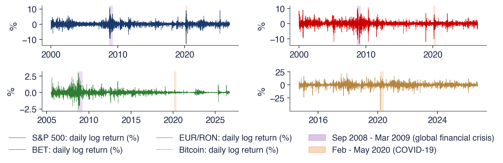
 TSA_ch5_stylised_facts