Bucharest University of Economic Studies IDA Institute Digital Assets Blockchain Research Center AI4EFin Artificial Intelligence for Energy Finance Romanian Academy, Institute for Economic Forecasting MSCA Digital Finance
The question of the chapter is how to model several series that move together, such as output, prices and interest rates, or three stock markets, and what such a joint model can say about which series leads which. The answer is the vector autoregression: one equation for each variable, in which every variable depends on the past of all the variables. The univariate autoregressions of Chapter 2 are the special case with a single variable, and the stationarity tests of Chapter 3 decide whether a series enters the VAR in levels or in differences.
The route has three stages. The first moves from one series to several: vector processes, cross-correlations, the VAR(\(p\)) model and its stability. The second estimates the model, chooses the number of lags and checks the residuals, then tests Granger causality and its pitfalls. The third uses the estimated model: impulse responses, the variance decomposition, forecasts and, finally, the idea of a structural VAR in the form proposed by Sims (1980). Seminar 6 precedes this lecture and works with the same data.
In brief
Question: when several series move together (output, prices, interest rates; three stock markets), how do we model them jointly, and what can we learn about who leads whom?
one equation per variable, each with the past of all variables: the vector autoregression (VAR)
Route of the chapter
from one series to several: vector processes and cross-correlations; the VAR\((p)\) model and its stability
estimation, lag selection and diagnostics; Granger causality and its pitfalls
impulse responses, variance decomposition, forecasts; the structural VAR idea of Sims (1980)
The outcomes follow the route. On the side of the model, the reader should be able to write a VAR(\(p\)) both as a matrix equation and as a set of scalar regressions, count its coefficients, check its stability with the eigenvalues of the companion matrix and compute the mean to which a stable VAR returns. On the side of estimation, the reader estimates a VAR by ordinary least squares (OLS), chooses the lag order with the information criteria AIC, BIC and HQ, and tests whether the residuals are white noise.
The remaining outcomes concern the uses of the model. Granger causality is tested with an \(F\) test, and its result is stated as a statement about predictability, never about cause and effect. Impulse responses and the forecast error variance decomposition (FEVD) require uncorrelated shocks; the reader computes them with the Cholesky decomposition and explains why the ordering of the variables is an assumption that can change the results. Finally, the reader produces VAR forecasts with intervals and compares them out of sample with a random walk and univariate autoregressions.
In brief
Write a VAR\((p)\) in matrix form and equation by equation, and count its parameters
Check stability with the eigenvalues of the companion matrix, and compute the mean of a stable VAR
Estimate a VAR by OLS, choose \(p\) with AIC, BIC and HQ, and check the residuals
Test Granger causality and explain what it does not prove
Compute and read orthogonalised impulse responses and variance decompositions, and explain why the ordering matters
Forecast with a VAR and compare it fairly with univariate benchmarks
The course textbook is Huang and Petukhina (2022), whose Chapter 7 covers multivariate time series. Hyndman and Athanasopoulos (2021), Section 12.3, gives a short, free introduction to VAR models with a forecasting perspective. The theory is in Lütkepohl (2005), Chapters 2–4, the standard reference for VAR models, and in Hamilton (1994), Chapter 11. Stock and Watson (2001) is an accessible survey of the method, and it serves as the case study of the last main section.
The computations use the VAR class of statsmodels in Python: select_order for the information criteria, fit for the OLS estimates, test_whiteness for the portmanteau test, irf and fevd for impulse responses and variance decompositions, and forecast_interval for forecasts with intervals. The Quantlets of the chapter reproduce every chart and table, and the lecture notebook runs in Google Colab.
There occurs on some occasions a difficulty in deciding the direction of causality between two related variables and also whether or not feedback is occurring. Testable definitions of causality and feedback are proposed and illustrated by use of simple two-variable models.
The models of Chapters 1–5 describe one series at a time: its mean, its autocorrelations, its variance. Economic variables, however, are rarely isolated. The central bank sets the interest rate after looking at inflation and output; inflation responds, with a delay, to the interest rate; the stock market in Bucharest opens the morning after Wall Street has closed. A forecast of the interest rate that ignores inflation throws away information, and a regression of inflation on the interest rate that treats the interest rate as given ignores the fact that the interest rate itself responds to inflation.
This chapter models several series jointly with the vector autoregression (VAR): one equation per variable, each variable regressed on the past of all the variables. Sims (1980) proposed the VAR as an alternative to the large macroeconomic models of the 1970s, and it became the standard tool of central banks. The same model answers four questions: does one series help to forecast another (Granger causality), how does each variable respond over time to a shock in another (impulse responses), which shocks account for the forecast uncertainty of each variable (variance decomposition), and what the joint forecasts are. The quotation above, from Granger (1969), states the first of these questions.
The running examples are a quarterly VAR for Romania, with real GDP growth, inflation and the three-month interbank rate ROBOR 3M, from 2005 Q1 to 2026 Q2; a daily VAR for the returns of the S&P 500, the DAX and the BET from 2000 to 2026; and the three-variable VAR for the United States of Stock and Watson (2001). In the Romanian VAR, past GDP growth and past inflation help to forecast ROBOR, and after an inflation shock ROBOR rises for about a year and stays higher for three. On the markets, yesterday's return in New York helps to forecast today's returns in Frankfurt and Bucharest, because of the closing hours.
Romania: real GDP growth quarter on quarter and the unemployment rate, seasonally adjusted (Eurostat); 12-month HICP inflation and ROBOR 3M (Eurostat); the EUR/RON reference rate of the BNR, monthly mean.
What you will be able to do
Write a VAR(\(p\)) in matrix form and equation by equation, and count its parameters.
Check stability with the eigenvalues of the companion matrix and compute the mean of a stable VAR.
Estimate a VAR by OLS, choose \(p\) with AIC, BIC and HQ, and test the residuals.
Test Granger causality and explain what it does not prove.
Compute and interpret orthogonalised impulse responses and the forecast error variance decomposition, and explain why the ordering of the variables matters.
Forecast with a VAR and compare the forecasts fairly with univariate benchmarks.
Chapter plan
From one series to severalVector time series, autocovariance matrices and the cross-correlation function on Romanian and market data.
The VAR(p) modelThe model in matrix form and equation by equation, a worked example, the number of parameters and Sims's proposal.
Stationarity and the companion formThe stability condition, the mean and variance of a stable VAR, the companion matrix and the moving-average representation.
Estimation and lag selectionOLS equation by equation, the AIC, BIC and HQ criteria and the estimated Romanian VAR(2).
Residual diagnosticsThe multivariate portmanteau test, normality and the residuals of the Romanian VAR.
Granger causalityThe definition, the F test, results for Romania and for three stock markets, and three pitfalls.
Impulse responsesOrthogonalisation with the Cholesky decomposition, the role of the ordering and generalised responses.
SummaryKey ideas, formulas and self-assessment questions.
From one series to several
This section introduces the objects of multivariate time-series analysis. It starts with four Romanian macroeconomic series and the questions they raise, defines a vector time series and its autocovariance matrices, and introduces the cross-correlation function, the multivariate analogue of the autocorrelation function. Two applications, one on daily stock returns and one on Romanian inflation and interest rates, show what the cross-correlation function reveals and where it stops being informative. The section ends with the argument for a single model of all the series.
Question for the room Move the start of the window to 2015. What does the correlation between inflation and ROBOR 3M become?
Answer
0.89, against 0.66 over 2005–2026. After 2015 the two series rose and fell together (inflation reached 13.6% in November 2022, ROBOR 3M 8.0% in October 2022), and the 2008 episode, when ROBOR reached 18.2% in the liquidity crisis, has left the window. The correlation between the levels of two persistent series depends strongly on the sample and does not say which of them leads the other.
The chart shows four panels of Romanian data. The top-left panel is the growth of real gross domestic product (GDP) over the previous quarter, seasonally adjusted, in percent. The top-right panel shows two series on one axis: the 12-month inflation rate of the harmonised index of consumer prices (HICP), in red, and ROBOR 3M, the three-month interest rate at which Romanian banks offer interbank deposits, in blue, in percent per year. The bottom panels show the seasonally adjusted unemployment rate and the EUR/RON reference rate of the National Bank of Romania (BNR), as a monthly mean.
The series come from Eurostat and the BNR. GDP growth is a quarterly flow, while inflation, the interest rate, unemployment and the exchange rate are monthly; in the VAR of this chapter the monthly series are averaged over each quarter, so that all variables refer to the same periods. The main VAR uses three of the series, GDP growth, inflation and ROBOR 3M, which are the variables of a standard small model of monetary policy: activity, prices and the policy-related interest rate.
In brief
Real GDP growth (q/q) and unemployment rate, seasonally adjusted; 12-month HICP inflation; ROBOR 3M, the 3-month interbank rate; source: Eurostat; EUR/RON: the BNR reference rate
The most visible feature of the top-right panel is that inflation and ROBOR 3M rise and fall together. Their correlation over 2005 Q1 – 2026 Q2, computed on quarterly averages, is 0.66. Inflation reached its maximum of 13.6% in November 2022, after the energy price shock; ROBOR 3M reached 18.2% in October 2008, during the liquidity crisis of that autumn, when interbank rates spiked without a matching rise in inflation. A common movement of this kind is what a joint model has to explain.
GDP growth behaves differently: it fluctuates around a small positive mean with two large falls, −10.2% in 2009 Q1, in the global financial crisis, and −8.6% in 2020 Q2, in the pandemic. The most recent values are an inflation rate of 6.1% in August 2026, ROBOR 3M at 5.69%, an unemployment rate of 6.4% and an exchange rate of 5.26 lei per euro. The chart raises the two questions of the chapter: does inflation help to forecast the interest rate, and how does ROBOR react to an inflation surprise, and for how long? The first is answered by Granger causality, the second by impulse responses.
In brief
Inflation and ROBOR 3M rise and fall together: correlation 0.66 over 2005Q1–2026Q2 (quarterly means)
inflation peaked at 13.6% in November 2022; ROBOR 3M peaked at 18.2% in October 2008 (the 2008 liquidity squeeze)
GDP growth is noisy, with two deep falls: \(-\)10.2% in 2009Q1 and \(-\)8.6% in 2020Q2
A vector time series collects \(K\) series observed at the same dates into one column vector, \(\bY_t = (Y_{1t}, \dots, Y_{Kt})'\), where \(Y_{jt}\) is the value of series \(j\) at date \(t\) and the prime denotes the transpose. In the Romanian example, \(\bY_t = (g_t, \pi_t, i_t)'\) contains GDP growth, inflation and ROBOR 3M in quarter \(t\), so \(K = 3\). The vector of means is \(\boldsymbol{\mu} = E[\bY_t]\), of dimension \(K \times 1\), and the dependence over time is described by the autocovariance matrix at lag \(h\),\(\bGamma(h) = \Cov(\bY_t, \bY_{t-h}) = E[(\bY_t - \boldsymbol{\mu})(\bY_{t-h} - \boldsymbol{\mu})']\), a \(K \times K\) matrix.
The diagonal of \(\bGamma(h)\) contains the autocovariances of each series at lag \(h\), the objects of Chapter 1. The off-diagonal elements are the cross-covariances \(\gamma_{jk}(h) = \Cov(Y_{jt}, Y_{k,t-h})\), which measure how series \(j\) today is related to series \(k\)\(h\) periods earlier. The vector series is weakly stationary when \(\boldsymbol{\mu}\) and \(\bGamma(h)\) do not depend on \(t\), the direct extension of the univariate definition.
Unlike a univariate autocovariance, \(\bGamma(h)\) is not symmetric: \(\gamma_{12}(h)\) relates \(Y_1\) today to \(Y_2\) in the past, while \(\gamma_{21}(h)\) relates \(Y_2\) today to \(Y_1\) in the past, and the two can differ. The only symmetry is \(\bGamma(-h) = \bGamma(h)'\). This asymmetry is what makes questions of precedence possible: "\(Y_1\) leads \(Y_2\)" and "\(Y_2\) leads \(Y_1\)" are different statements, and the data can support one without the other.
In brief
Definition: \(\bY_t = (Y_{1t}, \dots, Y_{Kt})'\) collects \(K\) series observed at the same dates
example: \(\bY_t = (g_t, \pi_t, i_t)'\), GDP growth, inflation and ROBOR 3M of quarter \(t\); \(K = 3\)
\(Y_{jt}\): the value of series \(j\) at date \(t\); the prime \('\) denotes the transpose (a column vector)
Mean vector: \(\boldsymbol{\mu} = E[\bY_t]\), \(K \times 1\)
autocovariance matrix at lag \(h\): \(\bGamma(h) = \Cov(\bY_t, \bY_{t-h}) = E[(\bY_t - \boldsymbol{\mu})(\bY_{t-h} - \boldsymbol{\mu})']\), \(K \times K\)
diagonal: the autocovariances of each series (Chapter 1); off-diagonal: cross-covariances\(\gamma_{jk}(h) = \Cov(Y_{jt}, Y_{k,t-h})\)
Weak stationarity: \(\boldsymbol{\mu}\) and \(\bGamma(h)\) do not depend on \(t\)
\(\bGamma(h)\) is not symmetric, but \(\bGamma(-h) = \bGamma(h)'\): “\(Y_1\) leads \(Y_2\)” and “\(Y_2\) leads \(Y_1\)” are different statements
where \(\gamma_{yx}(k) = \Cov(y_t, x_{t-k})\) is the cross-covariance and \(\sigma_y\),\(\sigma_x\) are the standard deviations of the two series. A positive lag \(k\) pairs today's \(y\) with an earlier \(x\), so a large \(\rho_{yx}(k)\) for \(k > 0\) indicates that \(x\) leads \(y\); a large value for \(k < 0\) indicates that \(y\) leads \(x\). The sample version \(\hat\rho_{yx}(k)\) is the correlation of the pairs \((y_t, x_{t-k})\) in the data.
If the two series are independent white noise, \(\hat\rho_{yx}(k)\) is approximately Normal with mean 0 and variance \(1/T\), where \(T\) is the number of observations, which gives the reference bands \(\pm 1.96/\sqrt{T}\). The bands are valid only under that assumption. When both series are autocorrelated, the sample cross-correlations vary much more than \(1/\sqrt{T}\) suggests, and values outside the bands appear even when the series are independent. This is the same mechanism as the spurious regression of Chapter 3: persistence inflates apparent relations.
The CCF looks at one pair of series and one lag at a time. It cannot separate the information that \(x_{t-1}\) brings about \(y_t\) from the information that is already contained in \(y_{t-1}\), nor can it account for a third variable. A VAR looks at all the variables and all the lags together, which is why it replaces the CCF once the questions become precise.
the cross-correlation function (CCF): \(k > 0\): past \(x\) with today's \(y\) (\(x\) leads); \(k < 0\): \(y\) leads
\(\gamma_{yx}(k) = \Cov(y_t, x_{t-k})\): the cross-covariance; \(\sigma_y\), \(\sigma_x\): the standard deviations of the two series
Sample version: \(\hat\rho_{yx}(k)\), the correlation of the pairs \((y_t, x_{t-k})\)
if the two series are independent white noises, \(\hat\rho_{yx}(k) \approx N(0, 1/T)\), with \(T\) the number of observations: bands \(\pm 1.96/\sqrt{T}\)
with autocorrelated series the bands are too narrow: spurious lead–lag patterns (compare Chapter 3, spurious regression)
The CCF looks at one pair and one lag at a time; a VAR looks at all variables and all lags together
Cross-correlations: markets and Romanian macro data
Question for the room Start the daily returns in 2015. Is the correlation between yesterday’s DAX and today’s S&P 500 (k = −1) inside the band?
Answer
No: −0.058, outside the band ±0.037; over the whole sample it is −0.046, also outside the band ±0.024. The lead runs mainly from New York to Europe (0.135 at k = 1 since 2015, 0.171 over the whole sample), but not in one direction only: yesterday’s DAX also has a small negative correlation with today’s S&P 500. For the BET the value at k = −1 (−0.005 since 2015, −0.017 over the whole sample) stays inside the band.
The left panel uses daily log returns from 2000 to 2026, on the 6,433 days on which the three exchanges all traded. Each pair of bars shows \(\Corr(\text{DAX}_t, \text{S\&P}_{t-k})\) in turquoise and \(\Corr(\text{BET}_t, \text{S\&P}_{t-k})\) in red, for lags \(k\) from −5 to 5 days; the dashed lines are the bands \(\pm 1.96/\sqrt{T}\). Bars at positive \(k\) pair today's European return with an earlier S&P 500 return.
The right panel pairs quarterly ROBOR 3M with lags of inflation, \(\Corr(\text{ROBOR}_t, \pi_{t-k})\), for \(k\) from −8 to 8 quarters. Here there are no bands, because both series are persistent and the white-noise bands would be misleading. The two panels were chosen to contrast two situations: returns with almost no own memory, for which the CCF is easy to read, and persistent macroeconomic levels, for which it is not.
In brief
Left: daily log returns (EODHD), 6 433 common trading days, 2000–2026; bars: \(\Corr(\text{DAX}_t, \text{S\&P}_{t-k})\) and \(\Corr(\text{BET}_t, \text{S\&P}_{t-k})\). Right: quarterly ROBOR 3M against lags of inflation
For the BET, the correlation with the S&P 500 is 0.21 on the same day and 0.17 with the previous day's S&P 500 return (\(k = 1\)); in the opposite direction, at \(k = -1\), it is −0.02. The band is ±0.024, so the lag-1 value is far outside it, while the reverse value is inside. For the DAX, the same-day correlation is 0.59 and the lag-1 correlation 0.17; the reverse value, −0.046, is small and negative, just outside the band. Yesterday's return in New York is visible in today's returns in Frankfurt and Bucharest, much more strongly than the other way round.
The reason is the clock. Wall Street closes at 22:00 Frankfurt time, hours after the European exchanges. Part of what happens in New York on day \(t-1\) happens when Europe is already closed, and European prices absorb it only when they open on day \(t\). The lead of the S&P 500 is therefore a consequence of non-synchronous trading hours, a point that returns in the Granger tests.
For ROBOR and inflation, the largest correlation, 0.70, is at \(k = 2\) quarters, which suggests that inflation leads the interest rate by about half a year. Yet all the values are large: 0.34 at \(k = -4\) and 0.64 at \(k = 4\). Both series are persistent, so any lag of one is correlated with any nearby value of the other. The CCF alone cannot separate precedence from persistence; for that, the past of ROBOR itself must be controlled for, which is exactly what a VAR does.
In brief
BET with the S&P 500: 0.21 on the same day and 0.17 with the previous day (\(k = 1\)); with \(k = -1\): \(-\)0.02
the band is \(\pm\)0.024: yesterday's New York return is clearly visible in today's Bucharest and Frankfurt returns (DAX at \(k = 1\): 0.17); the reverse link is much weaker (DAX at \(k = -1\): \(-\)0.046, just outside the band)
reason: Wall Street closes at 22:00 in Frankfurt, after the European markets; its news reaches them the next morning
ROBOR with inflation: the largest correlation, 0.70, is at \(k = 2\) quarters (inflation leads)
but every value is large (0.34 at \(k = -4\), 0.64 at \(k = 4\)): two persistent series; the CCF alone cannot separate lead from persistence
The univariate models of Chapters 2–3 forecast each series from its own past. They ignore the possibility that last quarter's inflation helps to forecast this quarter's interest rate, even though the cross-correlations suggest that it does. If such information exists, a model that uses it can forecast better and can describe how the variables influence each other.
A single regression is not the answer either. A regression of \(\pi_t\) on \(i_t\) treats the interest rate as given, or exogenous, determined outside the model. With feedback, the central bank reacts to inflation and inflation reacts to the interest rate, so both variables are endogenous: they are determined jointly inside the system, and the regression coefficient mixes the two directions of influence.
A VAR treats all variables symmetrically: each depends on the past of all the others, and none is declared exogenous in advance. Writing it requires no economic theory beyond the choice of the variables. Theory returns when the shocks are interpreted, in the section on impulse responses, because to say that a movement in ROBOR is a "monetary policy shock" requires assumptions that the data alone cannot provide.
In brief
Univariate models (Chapters 2–3) forecast each series from its own past
they ignore that last quarter's inflation may help to forecast this quarter's interest rate
Feedback: the central bank reacts to inflation, inflation reacts to the interest rate
a single regression of \(\pi_t\) on \(i_t\) treats \(i_t\) as given (exogenous); here both are endogenous, determined inside the system
A VAR treats all variables symmetrically: each depends on the past of all
no economic theory is needed to write it down; theory comes back when we interpret shocks (Section 7)
A vector series \(\bY_t\) has a vector of means and autocovariance matrices \(\bGamma(h)\), whose off-diagonal elements are cross-covariances. These matrices are not symmetric, and \(\bGamma(-h) = \bGamma(h)'\); this asymmetry is what allows one series to lead another. The cross-correlation function \(\rho_{yx}(k)\) measures such leads one pair and one lag at a time, with \(k > 0\) meaning that \(x\) leads.
On daily data, the S&P 500 leads the DAX and the BET by one day, because of the closing hours. On quarterly Romanian data, inflation and ROBOR are strongly correlated at all lags, so the CCF cannot tell lead from persistence. The feedback between the variables calls for a joint model, the VAR.
In brief
A vector series \(\bY_t\) has a mean vector and autocovariance matrices \(\bGamma(h)\), with \(\bGamma(-h) = \bGamma(h)'\)
S&P 500 returns lead DAX and BET returns by one day
Feedback between variables calls for a joint model
Section summary
Several series observed together carry information that no univariate model uses: the past of one series can help to forecast another, and shocks can travel from one variable to the next. The cross-correlation function detects such links on simple data, but it fails when the series are persistent and when more than two variables interact. The next section introduces the model that handles all variables and lags at once.
The VAR\((p)\) model
This section defines the vector autoregression of order \(p\) and shows how to read it, first in matrix form and then equation by equation. A worked example with two variables is solved by hand and then simulated, and the section counts the parameters that a VAR has to estimate, which explains why VARs are kept small. It ends with the historical argument of Sims (1980), which made the VAR the standard tool of empirical macroeconomics.
where \(\bc\) is a \(K \times 1\) vector of intercepts, \(\bA_1, \dots, \bA_p\) are \(K \times K\) coefficient matrices, and \(\bepsilon_t\) is vector white noise: \(E[\bepsilon_t] = \mathbf{0}\),\(E[\bepsilon_t\bepsilon_t'] = \bSigma\) and \(E[\bepsilon_t\bepsilon_s'] = \mathbf{0}\) for \(t \ne s\). Each row of (6.2) is a regression of one variable on a constant and on \(p\) lags of every variable.
The covariance matrix \(\bSigma\) is in general not diagonal: the shocks of different equations are correlated at the same date. In the Romanian VAR, a quarter with an unexpected rise in inflation tends also to be a quarter with an unexpected rise in ROBOR. Shocks at different dates, by contrast, are uncorrelated; all the dynamics, the way the past affects the present, is in the matrices \(\bA_j\).
With \(K = 1\),(6.2) is the AR(\(p\)) model of Chapter 2. The form (6.2) is called the reduced form: it describes the joint behaviour of the data, the forecasts and the forecast errors, but its shocks \(\bepsilon_t\) are not economic shocks such as a monetary policy decision. The section on structural VARs shows what must be added to give the shocks an economic meaning.
With two variables and one lag, the matrix equation contains a \(2 \times 2\) matrix \(\bA\) with elements \(a_{11}, a_{12}, a_{21}, a_{22}\). Multiplying it out gives two ordinary regressions: \(y_{1t} = c_1 + a_{11}y_{1,t-1} + a_{12}y_{2,t-1} + \varepsilon_{1t}\) and \(y_{2t} = c_2 + a_{21}y_{1,t-1} + a_{22}y_{2,t-1} + \varepsilon_{2t}\). The two equations have the same regressors, the lagged values of both variables, but different coefficients and different shocks.
The indices follow a fixed rule: \(a_{jk}\) is the effect of \(y_{k,t-1}\) on \(y_{jt}\), so the row gives the equation and the column the regressor. The diagonal elements \(a_{11}\) and \(a_{22}\) measure how each variable depends on its own past, as in an AR(1). The off-diagonal elements carry the interaction. If \(a_{12} = a_{21} = 0\), the VAR splits into two separate AR(1) models (linked only through the correlation of their shocks); if \(a_{12} \ne 0\), the past of \(y_2\) helps to forecast \(y_1\), which is the property that the Granger test examines.
The example has \(\bc = (1.2, 0.6)'\),\(\bA\) with rows \((0.5, 0.2)\) and \((0.3, 0.4)\), and a shock covariance matrix \(\bSigma\) with variances 1 and covariance 0.5. Equation by equation, \(y_{1t} = 1.2 + 0.5y_{1,t-1} + 0.2y_{2,t-1} + \varepsilon_{1t}\) and \(y_{2t} = 0.6 + 0.3y_{1,t-1} + 0.4y_{2,t-1} + \varepsilon_{2t}\). The coefficient \(a_{21} = 0.3\) says that one extra unit of \(y_1\) in the previous period raises \(y_2\) by 0.3 today, holding \(y_2\)'s own past fixed. Since the variances are 1, the covariance 0.5 is also the correlation of the two shocks.
The forecast for the next period sets the future shock to its mean, zero. From \(\bY_T = (5, 2)'\),\(\hat\bY_{T+1} = \bc + \bA\bY_T\): for \(y_1\),\(1.2 + 0.5 \cdot 5 + 0.2 \cdot 2 = 4.10\); for \(y_2\),\(0.6 + 0.3 \cdot 5 + 0.4 \cdot 2 = 2.90\). The two-step forecast applies the same rule to the one-step forecast, \(\hat\bY_{T+2} = \bc + \bA\hat\bY_{T+1} = (3.83, 2.99)'\).
The forecasts move from the starting values towards the mean of the process, \(\boldsymbol{\mu} = (3.50, 2.75)'\), which the next section computes. \(y_1\) starts above its mean and falls towards it; \(y_2\) starts below and rises. Both movements are the multivariate version of the reversion to the mean of a stationary AR(1).
Question for the room Move a₂₁ to 0.6 (λ₁ = 0.8). What is the response of y₁ after 5 periods, Φ₁₁(5)?
Answer
0.187, not 0.8⁵ = 0.328. Φ₁₁(h) = 0.571·0.8ʰ + 0.429·0.1ʰ: the dominant component enters e₁ with weight 0.571, and the ratio Φ₁₁(h)/Φ₁₁(h−1) approaches 0.8 only after a few periods. The same holds in the lecture’s example: Φ₁₁(5) = 0.6·0.7⁵ + 0.4·0.2⁵ = 0.101, so after 5 periods about 0.10 of the initial effect is left; 0.7⁵ ≈ 0.17 is the factor by which the dominant component shrinks, not the response.
The left panel shows 200 periods simulated from the VAR(1) of the worked example, with \(y_{1t}\) in dark blue, \(y_{2t}\) in red and the two means as dashed and dotted horizontal lines. The right panel shows the impulse responses of the model: the paths of \(y_1\) and \(y_2\) after a unit shock in \(\varepsilon_1\) at horizon \(h = 0\), with all other shocks set to zero. These paths are the first column of the matrix \(\bA^h\), for \(h = 0, \dots, 10\).
At \(h = 0\) the shock moves only \(y_1\), by 1, and \(y_2\) is at 0; at \(h = 1\),\(y_1\) is at \(a_{11} = 0.5\) and \(y_2\) at \(a_{21} = 0.3\). After that, both responses decline together towards zero. The right panel ignores the correlation between the shocks: it shows what a shock to \(\varepsilon_1\) alone does, a question taken up again in the section on impulse responses.
In brief
Left: 200 periods of the VAR(1) of the previous slide, with its two means; right: the responses of \(y_1\) and \(y_2\) to a unit shock in \(\varepsilon_1\) at \(h = 0\), the columns of \(\bA^h\)
The two simulated series fluctuate around their means and move together: their sample correlation is 0.75. There are two sources of this common movement. The shocks are correlated, with correlation 0.5, so the two series are pushed in the same direction in the same period. The cross effects \(a_{12} = 0.2\) and \(a_{21} = 0.3\) then pass each movement from one series to the other in the next period, which raises the correlation above that of the shocks.
A unit shock to \(y_1\) reaches \(y_2\) after one period, through \(a_{21} = 0.3\), and then both responses die out. The speed at which they die out is governed by the largest eigenvalue of \(\bA\), 0.7: after a few periods, each response shrinks by a factor of about 0.7 per period. Five periods after the shock, the response of \(y_1\) is 0.10 and that of \(y_2\) is also 0.10. The second eigenvalue, 0.2, affects only the first periods, because \(0.2^h\) vanishes quickly.
In brief
The two series wander around their means and move together: sample correlation 0.75
two sources of co-movement: the correlated shocks (\(\Corr = 0.5\)) and the cross effects \(a_{12}\), \(a_{21}\)
A unit shock to \(y_1\) reaches \(y_2\) one period later (\(a_{21} = 0.3\)), then both fade
the decay is governed by the largest eigenvalue of \(\bA\), 0.7: \((\bA^h)_{11} = 0.6 \cdot 0.7^h + 0.4 \cdot 0.2^h\), so after 5 periods 0.10 of the shock remains in \(y_1\)
A VAR(\(p\)) with \(K\) variables and an intercept has \(K\) intercepts and \(p\) matrices of \(K^2\) coefficients, \(K + pK^2\) coefficients in total, plus \(K(K+1)/2\) distinct elements of \(\bSigma\). Each equation has \(1 + pK\) regressors. The Romanian VAR with \(K = 3\) and \(p = 2\) has \(3 + 2 \cdot 9 = 21\) coefficients, estimated on 84 quarters, so each equation estimates 7 coefficients from 84 observations.
The number grows with the square of \(K\), the curse of dimensionality of VAR models. With \(K = 5\) and \(p = 4\), the model has \(5 + 4 \cdot 25 = 105\) coefficients. With 25 years of quarterly data, 100 observations, each equation has 21 regressors and 79 residual degrees of freedom: the estimates are possible but imprecise, and the forecasts suffer from the estimation error.
For this reason, VARs in practice are small, with 3 to 6 variables and few lags, and their individual coefficients have large standard errors. They are rarely interpreted one by one. The model is summarised instead by joint tests, impulse responses and forecasts, which combine many coefficients into one statement about the system.
In brief
A VAR\((p)\) with \(K\) variables and a constant: \(K + pK^2\) coefficients, plus \(K(K+1)/2\) in \(\bSigma\)
each equation has \(1 + pK\) regressors
Romanian VAR: \(K = 3\), \(p = 2\): \(3 + 2 \cdot 9 = 21\) coefficients estimated on 84 quarters
The curse of dimensionality: \(K = 5\), \(p = 4\): \(5 + 4 \cdot 25 = 105\) coefficients
with 25 years of quarterly data (100 observations) each equation has 21 regressors and 79 residual degrees of freedom
Hence small VARs (3–6 variables), few lags, and estimates with large standard errors; individual coefficients are rarely interpreted
In the 1970s, macroeconomic forecasting relied on large systems of equations, each built from economic theory. Sims (1980) argued that the restrictions these models imposed to identify their equations were "incredible": decisions about which variables are exogenous and which lags have zero coefficients were made without evidence, and expectations made many of them untenable. His proposal was to start from an unrestricted VAR, in which every variable depends on the past of every variable, and to add only the minimal assumptions needed to interpret the shocks.
The VAR became the standard instrument of central banks for forecasting and for measuring the effects of monetary policy. In 2011, Christopher Sims received the Nobel Memorial Prize in Economic Sciences, together with Thomas Sargent, "for their empirical research on cause and effect in the macroeconomy". The photograph shows Sims in 2011.
A VAR(\(p\)) writes each variable as a linear function of a constant and \(p\) lags of all variables, plus a vector white-noise shock with covariance \(\bSigma\). The coefficient \(a_{jk}\) is the effect of the lag of variable \(k\) in the equation of variable \(j\), and \(\bSigma\) captures the correlation of the shocks within a period.
The model has \(K + pK^2\) coefficients, so \(K\) and \(p\) are kept small. Sims (1980) proposed the VAR as an alternative to the "incredible" restrictions of the large models of his time, and it remains the reference model for the joint dynamics of a few series.
In brief
\(\bY_t = \bc + \sum_{j=1}^{p}\bA_j\bY_{t-j} + \bepsilon_t\), \(\bepsilon_t\) white noise with covariance \(\bSigma\)
\(a_{jk}\): effect of the lag of variable \(k\) in the equation of variable \(j\)
\(K + pK^2\) coefficients: keep \(K\) and \(p\) small
Sims (1980): VARs as an alternative to “incredible” restrictions
Section summary
The VAR(\(p\)) extends the autoregression from one series to several: the same lagged regressors appear in every equation, and the off-diagonal coefficients carry the interaction between variables. The worked example showed how forecasts are computed and how a shock dies out; the parameter count showed why the model must remain small. The next section gives the condition under which the shocks die out at all.
Stationarity and the companion form
A VAR is useful for forecasting and for impulse responses only if the effect of past shocks fades. This section derives the condition for that, the stability condition, first for a VAR(1) and then, through the companion form, for a VAR(\(p\)). It computes the mean and variance of a stable VAR, applies the condition to three estimated VARs, and writes a stable VAR as a moving average of past shocks, the representation behind impulse responses and forecast errors.
Substituting the VAR(1) \(\bY_t = \bc + \bA\bY_{t-1} + \bepsilon_t\) into itself \(h\) times gives \(\bY_t = \bc + \bA\bc + \dots + \bA^{h-1}\bc + \bA^h\bY_{t-h} + \sum_{j=0}^{h-1}\bA^j\bepsilon_{t-j}\). The value \(h\) periods ago enters through \(\bA^h\bY_{t-h}\), and a shock \(j\) periods ago through \(\bA^j\bepsilon_{t-j}\). The past is forgotten, and old shocks lose their influence, only if \(\bA^h \to \mathbf{0}\) as \(h\) grows.
This happens exactly when all eigenvalues \(\lambda\) of \(\bA\) satisfy \(|\lambda| < 1\), the stability condition. The eigenvalues are the roots of \(\det(\bA - \lambda\mathbf{I}) = 0\), where \(\mathbf{I}\) is the identity matrix; for \(K = 2\) this is the quadratic \(\lambda^2 - \mathrm{tr}(\bA)\lambda + \det(\bA) = 0\), with the trace \(\mathrm{tr}(\bA) = a_{11} + a_{22}\) and the determinant \(\det(\bA) = a_{11}a_{22} - a_{12}a_{21}\). The eigenvalues can be complex, so \(|\lambda|\) is the modulus. A stable VAR that started long ago is weakly stationary; the condition is the multivariate version of \(|\phi| < 1\) for the AR(1) of Chapter 2.
For the worked example, \(\mathrm{tr}(\bA) = 0.5 + 0.4 = 0.9\) and \(\det(\bA) = 0.5 \cdot 0.4 - 0.2 \cdot 0.3 = 0.14\), so \(\lambda^2 - 0.9\lambda + 0.14 = 0\). The discriminant is \(0.81 - 0.56 = 0.25\), so \(\lambda = (0.9 \pm 0.5)/2\), which gives \(\lambda_1 = 0.7\) and \(\lambda_2 = 0.2\). Both lie inside the unit circle, and the VAR is stable.
the past is forgotten only if \(\bA^h \to \mathbf{0}\)
Stability condition: all eigenvalues \(\lambda\) of \(\bA\) satisfy \(|\lambda| < 1\)
eigenvalues: the roots of \(\det(\bA - \lambda\mathbf{I}) = 0\); for \(K = 2\): \(\lambda^2 - \mathrm{tr}(\bA)\lambda + \det(\bA) = 0\)
\(\mathbf{I}\): the identity matrix; \(\mathrm{tr}(\bA) = a_{11} + a_{22}\): the trace; \(\det(\bA) = a_{11}a_{22} - a_{12}a_{21}\): the determinant; \(|\lambda|\): the modulus (eigenvalues can be complex)
a stable VAR is weakly stationary (if it started long ago); this is the multivariate version of \(|\phi| < 1\) (Chapter 2)
For a stationary VAR(1), the mean is the same at every date. Taking expectations of both sides of the model gives \(\boldsymbol{\mu} = \bc + \bA\boldsymbol{\mu}\), since \(E[\bepsilon_t] = \mathbf{0}\), and solving,
In the example, \(\mathbf{I} - \bA\) has rows \((0.5, -0.2)\) and \((-0.3, 0.6)\) and determinant \(0.5 \cdot 0.6 - 0.2 \cdot 0.3 = 0.24\). Its inverse is \(1/0.24\) times the matrix with rows \((0.6, 0.2)\) and \((0.3, 0.5)\), and multiplying by \(\bc = (1.2, 0.6)'\) gives \(\boldsymbol{\mu} = (3.50, 2.75)'\). These are the levels towards which the forecasts of the worked example moved.
The variance matrix \(\bGamma(0)\) satisfies \(\bGamma(0) = \bA\bGamma(0)\bA' + \bSigma\), a discrete Lyapunov equation: the variance today is the variance transmitted from yesterday plus the variance of the new shock. Lagged autocovariances follow as \(\bGamma(h) = \bA^h\bGamma(0)\). The equation is solved by stacking the columns of a matrix into one vector, the operation \(\mathrm{vec}\), and using the Kronecker product \(\otimes\):\(\mathrm{vec}\,\bGamma(0) = (\mathbf{I} - \bA \otimes \bA)^{-1}\mathrm{vec}\,\bSigma\).
In the example, \(\bGamma(0)\) has variances 1.75 and 1.73 and covariance 1.22. Both variances exceed the variance of the shocks, 1, because the dynamics accumulate past shocks: today's value contains today's shock and the decaying effects of all earlier ones. The implied correlation of the two series, \(1.22/\sqrt{1.75 \cdot 1.73} \approx 0.70\), is larger than the correlation of the shocks, 0.5, which is the cross-effect mechanism seen in the simulation.
In brief
Mean: take expectations, \(\boldsymbol{\mu} = \bc + \bA\boldsymbol{\mu}\), so \(\boldsymbol{\mu} = (\mathbf{I} - \bA)^{-1}\bc\)
A VAR(\(p\)) can be rewritten as a VAR(1) by stacking \(p\) consecutive vectors into one, \(\boldsymbol{\xi}_t = (\bY_t', \bY_{t-1}', \dots, \bY_{t-p+1}')'\), of dimension \(Kp\). Then \(\boldsymbol{\xi}_t = \boldsymbol{\nu} + \mathbf{F}\boldsymbol{\xi}_{t-1} + \mathbf{v}_t\), where \(\boldsymbol{\nu}\) is \(\bc\) followed by zeros, \(\mathbf{v}_t\) is \(\bepsilon_t\) followed by zeros, and \(\mathbf{F}\) is the \(Kp \times Kp\) companion matrix. For \(p = 2\):
The first block of rows is the VAR(2) itself; the second block is the identity \(\bY_{t-1} = \bY_{t-1}\), which carries the lag forward.
Everything shown for the VAR(1) now applies to \(\boldsymbol{\xi}_t\). A VAR(\(p\)) is stable when all \(Kp\) eigenvalues of \(\mathbf{F}\) have modulus below 1. Equivalently, all roots \(z\) of \(\det(\mathbf{I}_K - \bA_1z - \dots - \bA_pz^p) = 0\), which are complex numbers in general, lie outside the unit circle; the eigenvalues of \(\mathbf{F}\) are the reciprocals of these roots.
The companion matrix is needed because the eigenvalues of \(\bA_1\) alone say nothing about the stability of a VAR(2). The second lag can make a system explosive even when \(\bA_1\) is small, or stable when \(\bA_1\) alone would suggest otherwise, as the univariate AR(2) already showed in Chapter 2.
then \(\boldsymbol{\xi}_t = \boldsymbol{\nu} + \mathbf{F}\boldsymbol{\xi}_{t-1} + \mathbf{v}_t\): every VAR\((p)\) is a VAR(1) in \(\boldsymbol{\xi}_t\)
\(\boldsymbol{\nu}\): \(\bc\) followed by zeros; \(\mathbf{v}_t\): \(\bepsilon_t\) followed by zeros; \(\mathbf{F}\): the \(Kp \times Kp\) companion matrix
Question for the room With p = 5, the order chosen by AIC, what is the largest modulus and how many eigenvalues does the companion matrix have?
Answer
0.913, out of 15 eigenvalues (the companion matrix is 15 × 15), against 0.869 out of 6 for p = 2; a shock halves after 7.7 quarters, against 5.0. Extra lags add eigenvalues, and some with a large modulus (0.874, 0.836) come in complex pairs, i.e. oscillations that the VAR(2) does not have. With 48 coefficients on about 80 quarters, these oscillations may be estimation noise.
The chart plots, in the complex plane, the eigenvalues of the companion matrices of three estimated VARs, with the unit circle as reference. The horizontal axis is the real part and the vertical axis the imaginary part of each eigenvalue. The red circles are the 6 eigenvalues of the Romanian VAR(2) in GDP growth, inflation and ROBOR 3M (\(K = 3\),\(p = 2\)). The blue squares are the 12 eigenvalues of the US VAR(4) of the Stock–Watson case study, and the green triangles the 12 eigenvalues of a daily VAR(4) of the S&P 500, DAX and BET returns.
Complex eigenvalues come in conjugate pairs, symmetric about the horizontal axis. A point close to the circle belongs to a slowly decaying component of the dynamics; a point close to the origin to a component that vanishes almost at once.
In brief
Companion matrices: Romanian VAR(2) (GDP growth, inflation, ROBOR 3M; 6 eigenvalues), the US VAR(4) of Section 10 (12), the daily S&P 500, DAX and BET VAR(4) (12)
All three VARs are stable: all their eigenvalues lie inside the unit circle. The largest moduli are 0.869 for Romania, 0.969 for the United States and 0.464 for the markets. The largest modulus sets the speed at which shocks eventually die out: in the US VAR, \(0.97^{20} \approx 0.54\), so after 20 quarters about half of the slowest component of a shock is still present; in the market VAR, \(0.46^2 \approx 0.21\), so after two days only a fifth remains.
The macroeconomic VARs have eigenvalues close to 1, because inflation and interest rates are persistent; the VAR of daily returns has small eigenvalues, because returns have almost no memory. Complex pairs, such as those of the US VAR away from the real axis, produce damped oscillations in the impulse responses: a response that overshoots zero before settling.
An eigenvalue very close to 1 signals a possible unit root, and the stability of the estimated VAR may then hide a nonstationary system. If several variables share a unit root and move together in the long run, they are cointegrated, and the appropriate model is the vector error correction model of Chapter 7.
In brief
All three VARs are stable; largest moduli: Romania 0.869, US 0.969, markets 0.464
the largest modulus sets the speed at which shocks fade: \(0.97^{20} \approx 0.54\) after 20 quarters, \(0.46^{2} \approx 0.21\) after 2 days
Macro VARs have eigenvalues close to 1 (persistent inflation and interest rates); return VARs have small ones
complex pairs produce damped oscillations in the responses
An eigenvalue very close to 1 signals a unit root, perhaps cointegration: Chapter 7
where \(\bPhi_h\) is a \(K \times K\) matrix that weights the shock of \(h\) periods ago. For a VAR(1), \(\bPhi_h = \bA^h\), as the repeated substitution showed. For a VAR(\(p\)), the matrices follow the recursion \(\bPhi_h = \sum_{j=1}^{\min(h,p)}\bA_j\bPhi_{h-j}\), which starts from \(\bPhi_0 = \mathbf{I}\) and is easy to compute.
In the example, \(\bPhi_2 = \bA^2\) has rows \((0.31, 0.18)\) and \((0.27, 0.22)\). The first row, for instance, is \(0.5 \cdot 0.5 + 0.2 \cdot 0.3 = 0.31\) and \(0.5 \cdot 0.2 + 0.2 \cdot 0.4 = 0.18\).
The element \((j, k)\) of \(\bPhi_h\) is the effect on \(Y_{j,t+h}\) of a unit change in \(\varepsilon_{kt}\), holding all other shocks fixed. These are the impulse responses of the section on impulse responses. The same matrices give the forecast errors: the error of a forecast \(h\) steps ahead is the sum of the shocks that have not yet occurred, weighted by \(\bPhi_0, \dots, \bPhi_{h-1}\), which is the basis of the variance decomposition and of the forecast intervals.
In brief
A stable VAR can be written as an infinite moving average of the shocks (Wold, Chapter 1):
A VAR(1) is stable when all eigenvalues of \(\bA\) have modulus below 1; a VAR(\(p\)) when all eigenvalues of its companion matrix do. A stable VAR has the mean \(\boldsymbol{\mu} = (\mathbf{I} - \bA_1 - \dots - \bA_p)^{-1}\bc\), and its forecasts converge to it.
The moving-average form \(\bY_t = \boldsymbol{\mu} + \sum_h\bPhi_h\bepsilon_{t-h}\) is the basis of impulse responses and forecast errors. Estimated macroeconomic VARs have eigenvalues close to 1, so their shocks fade slowly.
In brief
VAR(1): stable if all eigenvalues of \(\bA\) have \(|\lambda| < 1\); VAR\((p)\): the same for the companion matrix
Mean \(\boldsymbol{\mu} = (\mathbf{I} - \bA_1 - \dots - \bA_p)^{-1}\bc\); forecasts converge to it
Moving-average form \(\bY_t = \boldsymbol{\mu} + \sum_h\bPhi_h\bepsilon_{t-h}\): the basis of impulse responses
Estimated macro VARs have eigenvalues close to 1
Section summary
Stability is the property that makes a VAR usable: it guarantees a mean to which forecasts return, a finite variance, and responses to shocks that fade. The companion form reduces every VAR(\(p\)) to a VAR(1), so one condition covers all cases, and the moving-average representation turns the coefficient matrices into the responses and forecast errors used later in the chapter. The next section estimates the coefficients from data.
Estimation and lag selection
This section shows that a VAR is estimated by running OLS on each equation separately, explains why nothing is lost by doing so, and introduces the information criteria used to choose the number of lags. It then applies both steps to the Romanian data and reads the estimated VAR(2).
Each equation of a VAR is a linear regression of \(Y_{jt}\) on a constant and on the lagged vectors \(\bY_{t-1}, \dots, \bY_{t-p}\). All \(K\) equations have the same \(1 + Kp\) regressors, and each is estimated by ordinary least squares (OLS) separately. The estimates are those of \(K\) separate regressions; no special software is needed.
One might expect that the correlation of the shocks across equations could be exploited, by estimating the system jointly with generalised least squares (GLS). For a VAR it cannot: when all equations have identical regressors, the GLS estimator of the system equals OLS equation by equation, exactly. The correlation of the shocks does not improve the estimates. With Normal shocks, OLS is also the maximum likelihood estimator, conditional on the first \(p\) observations.
The covariance matrix of the shocks is estimated from the residuals of all equations, \(\hat\bSigma = \frac{1}{T - Kp - 1}\sum_t\hat\bepsilon_t\hat\bepsilon_t'\), where \(\hat\bepsilon_t\) is the vector of residuals at date \(t\) and \(T - Kp - 1\) the residual degrees of freedom of each equation. Stationarity matters for inference: for stationary series, the usual \(t\) and \(F\) tests are valid in large samples, while for series with unit roots some of them are not, a point that returns in the Granger pitfalls.
In brief
Each equation is a linear regression of \(Y_{jt}\) on a constant and \(\bY_{t-1}, \dots, \bY_{t-p}\)
the same \(1 + Kp\) regressors in every equation; OLS (ordinary least squares) on each equation separately
OLS is enough: with identical regressors, system estimation (GLS, generalised least squares, on all equations) gives exactly the OLS estimates
the correlation of the shocks does not improve the estimates; under Normal errors OLS is also the maximum likelihood estimator
Covariance of the shocks: \(\hat\bSigma = \frac{1}{T - Kp - 1}\sum_t\hat\bepsilon_t\hat\bepsilon_t'\), from the residuals of all equations
\(\hat\bepsilon_t\): the vector of residuals at date \(t\); \(T - Kp - 1\): the residual degrees of freedom of each equation
stationarity matters: with stationary series the usual \(t\) and \(F\) tests are valid in large samples
The lag order is chosen by estimating VAR(\(p\)) for \(p = 0, 1, \dots, p_{\max}\) on the same sample, where \(p_{\max}\) is the largest order tried, and comparing information criteria. Let \(\tilde\bSigma(p)\) be the covariance matrix of the residuals of the VAR(\(p\)), divided by \(T\). The three criteria are
proposed by Akaike (1974),Schwarz (1978) and Hannan and Quinn (1979). The determinant \(\det\tilde\bSigma(p)\) is a generalised variance of the residuals, a measure of their joint "volume", and \(pK^2\) is the number of lag coefficients. The order with the smallest value is chosen.
The first term measures the fit: it falls as lags are added. The second is a penalty per coefficient. The penalties are ordered AIC < HQ < BIC for \(T \ge 16\), so BIC chooses the smallest \(p\) and AIC the largest, with HQ in between. BIC and HQ are consistent: as \(T \to \infty\) they find the true order with probability tending to one. AIC tends to choose too many lags, but the models it selects often forecast well.
The comparison must use a common sample. A VAR(6) loses six initial observations to the lags, a VAR(1) only one; if each model used all its available observations, the criteria would compare fits on different data.
In brief
Fit VAR\((p)\) for \(p = 0, \dots, p_{\max}\) on the same sample; \(\tilde\bSigma(p)\): residual covariance divided by \(T\)
Question for the room End the sample in 2019 (pmax = 6). Which order does HQ choose?
Answer
p = 5, like AIC; BIC still chooses p = 1. The common sample has only T = 54 quarters, and ln det Σ̃(5) = −0.446 is far below the value for p = 2 (0.970), because a VAR(5) has 48 coefficients for 54 observations and almost reproduces the data. The HQ penalty, 2 ln ln T = 2.767 per unit of pK²/T, does not offset it. In short samples the criteria can choose large orders: check how many degrees of freedom are left.
The chart shows the three criteria for the Romanian VAR in GDP growth, 12-month inflation and ROBOR 3M, from 2005 Q1 to 2026 Q2, for \(p = 0, \dots, 6\), all estimated on the common sample of 80 quarters. The horizontal axis is the lag order, the vertical axis the value of the criterion; the circled points mark the minimum of each criterion.
All three curves fall steeply from \(p = 0\) to \(p = 1\): one lag captures most of the persistence of inflation and ROBOR. After that the curves separate, because their penalties differ: BIC rises from \(p = 1\), HQ is almost flat with its minimum at 2, and AIC continues to decline slightly.
In brief
GDP growth, 12-month inflation and ROBOR 3M, 2005Q1–2026Q2; VAR\((p)\) for \(p = 0, \dots, 6\) on the common sample of 80 quarters; circles mark the minima
BIC chooses \(p = 1\), HQ \(p = 2\) and AIC \(p = 5\). The three criteria disagree, as they often do in short samples. The AIC values show why: 1.812 for \(p = 1\), 1.603 for \(p = 2\) and 1.523 for \(p = 5\). Beyond \(p = 2\) the curve is nearly flat, so the AIC minimum at 5 rests on a small improvement in fit that the penalty barely offsets.
A VAR(5) would have \(3 + 5 \cdot 9 = 48\) coefficients for about 80 quarters, 16 per equation, and its estimates would be very imprecise. The chapter uses \(p = 2\), the HQ choice, and then checks whether the residuals are white noise; if they were not, lags would be added.
The practical rule is to start from the criteria but not to stop at them. They are a guide to the trade-off between fit and the number of parameters; the residual diagnostics, the stability of the model and the purpose of the analysis decide the final order.
In brief
BIC chooses \(p = 1\), HQ \(p = 2\), AIC \(p = 5\): the three criteria disagree, as they often do in short samples
AIC: 1.812 at \(p = 1\), 1.603 at \(p = 2\), 1.523 at \(p = 5\): a flat curve after \(p = 2\)
\(p = 5\) would mean \(3 + 5 \cdot 9 = 48\) coefficients for about 80 quarters
we take \(p = 2\) (HQ), then check whether the residuals are white noise; if not, we add lags
A rule of thumb: start from the criteria, never stop at them
The table reports the OLS estimates of the VAR(2) on 84 quarters, 2005 Q3 – 2026 Q2. Each column is one equation, with the dependent variable in the header: GDP growth \(g_t\), inflation \(\pi_t\) and ROBOR 3M \(i_t\). Each row is one regressor: the intercept and the first and second lags of the three variables. Each cell gives the coefficient and, in parentheses, its \(t\) statistic; with 77 residual degrees of freedom, \(|t| > 1.99\) indicates significance at 5%. The model has 21 coefficients.
The last row gives the \(R^2\) of each equation: 0.16 for GDP growth, 0.90 for inflation and 0.93 for ROBOR. Below the table, the standard deviations of the residuals are 2.32 percentage points for \(g\), 1.09 for \(\pi\) and 0.87 for \(i\); they measure the size of the typical one-quarter forecast error of each equation. The correlation of the residuals of \(\pi\) and \(i\) is 0.25: inflation and ROBOR surprises tend to come together.
In brief
Regressor
equation \(g_t\)
equation \(\pi_t\)
equation \(i_t\)
constant
\(1.09\) (\(2.1\))
\(0.49\) (\(2.0\))
\(-0.11\) (\(-0.6\))
\(g_{t-1}\)
\(0.01\) (\(0.1\))
\(0.01\) (\(0.1\))
\(0.14\) (\(3.5\))
\(\pi_{t-1}\)
\(0.53\) (\(2.3\))
\(1.26\) (\(11.7\))
\(0.24\) (\(2.8\))
\(i_{t-1}\)
\(-0.73\) (\(-2.7\))
\(0.16\) (\(1.2\))
\(1.04\) (\(10.2\))
\(g_{t-2}\)
\(-0.08\) (\(-0.7\))
\(-0.03\) (\(-0.5\))
\(0.07\) (\(1.7\))
\(\pi_{t-2}\)
\(-0.41\) (\(-1.7\))
\(-0.35\) (\(-3.1\))
\(-0.17\) (\(-1.9\))
\(i_{t-2}\)
\(0.54\) (\(2.0\))
\(-0.16\) (\(-1.3\))
\(-0.12\) (\(-1.2\))
\(R^2\)
0.16
0.90
0.93
OLS on 84 quarters (2005Q3–2026Q2); \(t\)-statistics in parentheses; 21 coefficients
Residual standard deviations: 2.32 (\(g\)), 1.09 (\(\pi\)), 0.87 (\(i\)); residual correlation of \(\pi\) and \(i\): 0.25
Inflation is very persistent. Its equation has \(1.26\,\pi_{t-1} - 0.35\,\pi_{t-2}\), so the sum of its own lag coefficients is 0.91, close to 1. ROBOR is similar, with \(1.04\,i_{t-1}\). The \(R^2\) of 0.90 and 0.93 come mostly from the series' own past: a variable that changes slowly is well predicted by its last value, which says little about the other variables.
The ROBOR equation is where the cross effects are clearest. Past GDP growth (\(t = 3.5\)) and past inflation (\(t = 2.8\)) both enter with positive coefficients: the interest rate follows the economy, rising after strong growth and after high inflation. GDP growth, in contrast, is hard to forecast: its \(R^2\) is 0.16, and most of its variation is unpredictable from the past of the three variables.
Individual coefficients on correlated lags are unstable. In the GDP equation, \(i_{t-1}\) has −0.73 and \(i_{t-2}\) has 0.54: because \(i_{t-1}\) and \(i_{t-2}\) are almost the same variable, the data can determine their combined effect much better than each coefficient separately. The system is therefore interpreted through joint tests, impulse responses and forecasts, not coefficient by coefficient.
In brief
Inflation is very persistent: \(1.26\,\pi_{t-1} -0.35\,\pi_{t-2}\); ROBOR too: \(1.04\,i_{t-1}\)
\(R^2\) of 0.90 and 0.93: most of it is the series' own past
In the ROBOR equation, past GDP growth (\(t = 3.5\)) and past inflation (\(t = 2.8\)) matter: the interest rate follows the economy
GDP growth is hard to predict: \(R^2 = 0.16\)
Single coefficients of correlated lags are unstable (e.g. \(i_{t-1}\) and \(i_{t-2}\) with opposite signs in the \(g\) equation): read the system through tests, responses and forecasts, not one coefficient at a time
OLS equation by equation is efficient for a VAR, because all equations share the same regressors. The lag order is chosen with AIC, BIC or HQ, each equal to \(\ln\det\tilde\bSigma(p)\) plus a penalty, all compared on a common sample.
The chosen orders satisfy BIC ≤ HQ ≤ AIC; for the Romanian VAR they are 1, 2 and 5, and the chapter uses \(p = 2\). Persistence dominates the inflation and ROBOR equations, and the system is read through tests and responses rather than individual coefficients.
In brief
OLS equation by equation is efficient: all equations have the same regressors
AIC, BIC, HQ: \(\ln\det\tilde\bSigma(p)\) plus a penalty; compare on a common sample
BIC \(\le\) HQ \(\le\) AIC in the chosen \(p\); Romanian VAR: \(p = 2\)
Interpret the system, not single coefficients
Section summary
Estimating a VAR requires nothing beyond OLS, and choosing its order requires a criterion that weighs fit against the number of coefficients. The Romanian VAR(2) shows the typical picture of a small macroeconomic VAR: persistent inflation and interest rates, a hard-to-forecast output growth, and cross effects concentrated in the interest rate equation. The next section checks whether the model has captured the dynamics.
Residual diagnostics
If a VAR captures the dynamics of the data, its residuals should be white noise: uncorrelated over time and across equations at different dates. This section introduces the multivariate portmanteau test for this property and a test of normality, and applies both to the Romanian VAR(2).
The multivariate portmanteau test of Hosking (1980) tests the null hypothesis \(H_0\) that the residuals have no autocorrelation and no cross-correlation up to lag \(h\). Its statistic is
where \(\hat{\mathbf{C}}_j = \frac{1}{T}\sum_t\hat\bepsilon_t\hat\bepsilon_{t-j}'\) is the autocovariance matrix of the residuals at lag \(j\) and \(\mathrm{tr}\) is the trace. Each term is a matrix version of the squared autocorrelation, standardised by the residual covariance \(\hat{\mathbf{C}}_0\). Under \(H_0\),\(Q_h\) has approximately a \(\chi^2\) distribution with \(K^2(h - p)\) degrees of freedom: \(K^2\) correlations per lag, minus the \(K^2p\) coefficients already fitted. It is the multivariate Ljung–Box test of Chapter 2, and a small p-value means that the residuals are still autocorrelated.
Normality is checked with a multivariate Jarque–Bera test, following Jarque and Bera (1980), on the standardised residuals, which compares their skewness and kurtosis with those of the Normal distribution (0 and 3). Normality is not required for OLS to be consistent; it matters for exact intervals and in small samples.
If the portmanteau test rejects, the remedies are to add lags, to add a variable, or to model breaks and extreme observations with dummy variables. The stability of the estimated model, through its eigenvalues, is checked as well and, in long samples, the stability of the parameters over time.
\(H_0\): no autocorrelation and no cross-correlation of the residuals up to lag \(h\)
\(Q_h = T^2\sum_{j=1}^{h}\frac{1}{T - j}\mathrm{tr}(\hat{\mathbf{C}}_j'\hat{\mathbf{C}}_0^{-1}\hat{\mathbf{C}}_j\hat{\mathbf{C}}_0^{-1})\), \(\hat{\mathbf{C}}_j = \frac{1}{T}\sum_t\hat\bepsilon_t\hat\bepsilon_{t-j}'\): the residual autocovariance matrix at lag \(j\); \(\mathrm{tr}\): the trace
under \(H_0\): \(\chi^2\) with \(K^2(h - p)\) degrees of freedom; the multivariate Ljung–Box test (Chapter 2); a small p-value: the residuals are still autocorrelated
Normality: a multivariate Jarque–Bera test Jarque and Bera (1980) on the standardised residuals (skewness and kurtosis)
Normality is not needed for OLS; it matters for exact intervals and for small samples
If the portmanteau test rejects: add lags, add a variable, or model breaks and outliers (dummy variables)
also check stability (eigenvalues) and, for long samples, parameter stability over time
Question for the room Add dummies for 2009Q1 and 2020Q2. Does the Jarque–Bera test still reject normality of the residuals?
Answer
Yes: the statistic falls from 191 to 144 (χ²(6), p < 0.001). The dummies cancel the residuals of the two quarters, but other extreme values remain: ROBOR +3.5 in 2008Q4, inflation −3.7 in 2011Q3, GDP −5.9 in 2010Q3; the kurtosis of ROBOR stays 7.9. The portmanteau test even gets worse (Q₈ = 88.2, p = 0.002): removing two observations does not make the residuals Normal white noise.
The chart shows the residuals of the three equations of the Romanian VAR(2), from 2005 Q3 to 2026 Q2, as bars, one panel per equation. The dashed lines are at \(\pm 2\) residual standard deviations, \(\pm 2\hat\sigma\); for Normal residuals about 95% of the bars would lie inside them.
The three panels have different scales, because the residual standard deviations differ: 2.32 for GDP growth, 1.09 for inflation and 0.87 for ROBOR. What matters is the shape: whether the bars look like independent noise, and whether some quarters stand out far beyond the lines.
In brief
Residuals of the three equations, 2005Q3–2026Q2, with \(\pm 2\) residual standard deviations
A few quarters stand out. The largest residuals are −9.1 for GDP growth in 2020 Q2, the pandemic lockdown; +3.7 for ROBOR in 2008 Q4, the liquidity crisis of 2008; and −3.7 for inflation in 2011 Q3. These are events that a linear model of the past cannot foresee. They give the residuals heavy tails: the kurtosis is 6.5 for \(g\) and 7.9 for \(i\), against 3 for the Normal distribution, and the multivariate Jarque–Bera statistic is 191, with a p-value below 0.001. Normality is clearly rejected.
The portmanteau test gives \(Q_8 = 76.7\) with 54 degrees of freedom, p-value 0.023, and \(Q_{12} = 105.3\) with 90 degrees of freedom, p-value 0.130. White noise is rejected at 5% for 8 lags but not for 12. Some short-run correlation remains, partly because the 12-month inflation rates of consecutive quarters overlap: two quarters share most of the months over which inflation is measured, which creates autocorrelation by construction.
The consequence is a measured confidence in the model. The point estimates can be used, but the intervals of the following sections rely on large-sample approximations that are less accurate with heavy-tailed, slightly autocorrelated residuals. For the impulse responses, the chapter uses bootstrap bands, which do not assume Normal shocks.
In brief
Largest residuals: GDP \(-\)9.1 in 2020Q2 (the pandemic), ROBOR \(+3.7\) in 2008Q4 (the 2008 liquidity squeeze), inflation \(-\)3.7 in 2011Q3
kurtosis 6.5 (\(g\)) and 7.9 (\(i\)), against 3 under the Normal distribution: Jarque–Bera 191 (p \(<\) 0.001)
Portmanteau: \(Q_8 = 76.7\) (\(54\) d.f., p = 0.023); \(Q_{12} = 105.3\) (\(90\) d.f., p = 0.130)
borderline at 8 lags, fine at 12: some short-run correlation is left, partly from overlapping 12-month inflation rates
Consequence: point estimates are usable, but the intervals of the next sections rely on large-sample approximations; we use bootstrap bands for the responses
The portmanteau test has the null hypothesis that the residuals are white noise, and its statistic is compared with a \(\chi^2\) distribution with \(K^2(h - p)\) degrees of freedom. Normality usually fails in macroeconomic data, because crises produce extreme residuals.
The remedies for remaining autocorrelation are more lags, more variables, or dummy variables for crisis quarters. For the Romanian VAR(2) the residuals are acceptable at 12 lags, borderline at 8, and far from Normal.
Normality fails in macro data: crises produce outliers
Remedies: more lags, more variables, dummies for crisis quarters
Section summary
Residual diagnostics decide how much trust to place in what follows. The Romanian VAR(2) leaves a small amount of short-run correlation and has heavy-tailed residuals driven by the crises of 2008 and 2020, so its inferences are approximate and its bands are better computed by bootstrap. The next section uses the model to ask which variables help to forecast which.
Granger causality
Granger causality turns the question "does \(x\) lead \(y\)?" into a testable statement about forecasts. This section gives the definition of Granger (1969), the \(F\) test in a VAR, a worked example and results for the Romanian VAR and for three stock markets. It then shows three pitfalls: omitted variables, effects within the same period, and nonstationarity and expectations. Each limits what a significant or non-significant test can mean.
Granger (1969) defined causality in terms of forecasts. A variable \(x\) Granger-causes \(y\) if the past of \(x\) improves the forecast of \(y\) made from the past of \(y\) and of the other variables in the information set. Formally, the mean squared error (MSE) of the optimal forecast of \(y_{t+1}\) is smaller when \(x_t, x_{t-1}, \dots\) are added to the information used.
The definition is about predictability, not about cause and effect in the everyday sense. It rests on the principle that a cause comes before its effect; but coming before is not the same as causing, and the pitfalls at the end of this section show how a variable can help to forecast another without influencing it. The definition is also relative: it depends on which other variables are in the information set.
Between two variables there are four cases: no Granger causality in either direction; \(x \to y\) only; \(y \to x\) only; and feedback, \(x \leftrightarrow y\), when each helps to forecast the other. Clive Granger, shown in the photograph, received the Nobel Memorial Prize in Economic Sciences in 2003.
In a VAR(\(p\)), the forecast of \(y\) uses \(x\) only through the coefficients of \(x_{t-1}, \dots, x_{t-p}\) in the equation of \(y\). So \(x\) does not Granger-cause \(y\) exactly when all these coefficients are zero. In a bivariate VAR(2), the equation of \(y\) is \(y_t = c + a_{11}^{(1)}y_{t-1} + a_{12}^{(1)}x_{t-1} + a_{11}^{(2)}y_{t-2} + a_{12}^{(2)}x_{t-2} + \varepsilon_t\), where the superscript is the lag, and the null hypothesis is \(H_0: a_{12}^{(1)} = a_{12}^{(2)} = 0\).
The hypothesis is tested with the \(F\) test of linear regression:
\[F = \frac{(RSS_R - RSS_U)/p}{RSS_U/(T - Kp - 1)} \sim F(p, T - Kp - 1) \text{ under } H_0,\]
(6.8)
where \(RSS_U\) is the residual sum of squares of the equation of \(y\) with all regressors, the unrestricted model, and \(RSS_R\) the same sum without the lags of \(x\), the restricted model. Removing regressors always increases the RSS; the test asks whether it increases more than chance would explain. A large \(F\), with a small p-value, means that the lags of \(x\) carry information about \(y\), and \(H_0\) is rejected.
An equivalent form is the Wald test \(W = (\mathbf{R}\hat{\boldsymbol{\beta}})'[\mathbf{R}\hat{\mathbf{V}}\mathbf{R}']^{-1}(\mathbf{R}\hat{\boldsymbol{\beta}})\), approximately \(\chi^2(p)\) under \(H_0\). Here \(\hat{\boldsymbol{\beta}}\) are the estimated coefficients of the equation of \(y\),\(\mathbf{R}\) is the matrix that selects the tested ones, and \(\hat{\mathbf{V}}\) is the estimated covariance matrix of \(\hat{\boldsymbol{\beta}}\); in this setting \(W = pF\). Both versions require stationary variables.
In brief
In a VAR\((p)\), \(x\) does not Granger-cause \(y\) if all coefficients of \(x_{t-1}, \dots, x_{t-p}\) in the equation of \(y\) are zero
\(\hat{\boldsymbol{\beta}}\): the estimated coefficients of the equation of \(y\); \(\mathbf{R}\) selects the tested ones; \(\hat{\mathbf{V}}\): the estimated covariance of \(\hat{\boldsymbol{\beta}}\); both versions need stationary variables
Worked example: does GDP growth Granger-cause ROBOR?
The test uses the equation of \(i_t\) in the Romanian VAR(2), with \(T = 84\),\(K = 3\) and \(p = 2\). The unrestricted equation, with \(g_{t-1}\) and \(g_{t-2}\) among its regressors, has \(RSS_U = 58.27\); the restricted equation, without them, has \(RSS_R = 69.27\). Dropping the two lags of GDP growth increases the residual sum of squares by 11.0.
The statistic is \(F = \frac{(69.27 - 58.27)/2}{58.27/77} = \frac{5.498}{0.7568} = 7.26\). The numerator is the increase in the RSS per restriction; the denominator is the residual variance of the unrestricted equation, with \(84 - 6 - 1 = 77\) degrees of freedom. Under \(H_0\),\(F\) follows the \(F(2, 77)\) distribution, whose 5% critical value is 3.12; the p-value is 0.001.
The decision is to reject \(H_0\): past GDP growth helps to forecast ROBOR 3M, given the past of inflation and of ROBOR. The result is compatible with a central bank that tightens monetary conditions when the economy grows fast, but the test establishes only the predictive link.
In brief
Equation of \(i_t\) in the Romanian VAR(2), \(T = 84\), \(K = 3\), \(p = 2\)
The table reports all six tests between pairs of the three variables in the VAR(2). Each row names the variable whose lags are tested (the cause), the equation in which they are tested (the effect), the \(F\) statistic and its p-value. All tests are \(F(2, 77)\), on 2005 Q3 – 2026 Q2, with the 5% critical value 3.12; each controls for the lags of the third variable.
Three relations are significant at 5%: GDP growth → ROBOR (\(F = 7.26\), p = 0.001), inflation → ROBOR (\(F = 4.74\), p = 0.011) and ROBOR → GDP growth (\(F = 4.02\), p = 0.022). Inflation → GDP growth is borderline, with p = 0.059. GDP growth → inflation (p = 0.853) and ROBOR → inflation (p = 0.417) are far from significant.
In brief
Cause
Effect
\(F\)
p
GDP growth
inflation
0.16
0.853
GDP growth
ROBOR 3M
7.26
0.001
inflation
GDP growth
2.94
0.059
inflation
ROBOR 3M
4.74
0.011
ROBOR 3M
GDP growth
4.02
0.022
ROBOR 3M
inflation
0.89
0.417
\(F(2, 77)\) tests in the VAR(2), 2005Q3–2026Q2; 5% critical value 3.12
Significant at 5%: GDP growth \(\to\) ROBOR, inflation \(\to\) ROBOR, ROBOR \(\to\) GDP growth
The interest rate follows the economy: past growth and past inflation both help to forecast ROBOR. This is the pattern of a reaction function, in which the central bank responds to inflation and to economic activity. The test alone cannot prove that this is the rule of the BNR: ROBOR is a market rate, and banks may anticipate the same information without any policy decision.
ROBOR does not Granger-cause inflation, with p = 0.417: there is no evidence that past interest rates improve the forecast of inflation. This does not mean that monetary policy is ineffective. The effect may be slow and spread over many quarters, small relative to the noise in inflation, or already anticipated, so that it shows up in the same quarter rather than with a lag. "Not significant" means that the test cannot separate the effect from noise in this sample, not that it is zero.
ROBOR → GDP growth, with p = 0.022, says that higher interest rates precede weaker growth, the expected direction of a monetary tightening. The result depends on the information set: in a bivariate VAR with only GDP growth and ROBOR, the p-value is 0.063.
In brief
The interest rate follows the economy: past growth and past inflation help to forecast ROBOR
the pattern of a reaction function (the central bank responds to inflation and activity); the test alone cannot prove it is the BNR's rule
ROBOR does not Granger-cause inflation (p = 0.417): no evidence that past rates improve inflation forecasts
this does not say that monetary policy is ineffective: the effect may be slow, small relative to the noise, or already anticipated
ROBOR \(\to\) GDP growth (p = 0.022): higher rates come before weaker growth; in the bivariate VAR (GDP, ROBOR) alone the p-value is 0.063
Markets: does New York lead Frankfurt and Bucharest?
The table reports Granger tests in a VAR(4) for the daily log returns of the S&P 500, the DAX and the BET, on 6,429 days from 2000 to 2026. The order 4 follows the specification of Diebold and Yilmaz (2012); HQ would choose \(p = 2\) and AIC \(p = 8\). The tests are \(F(4, \cdot)\), with four restrictions each, and the very large sample makes even small effects significant.
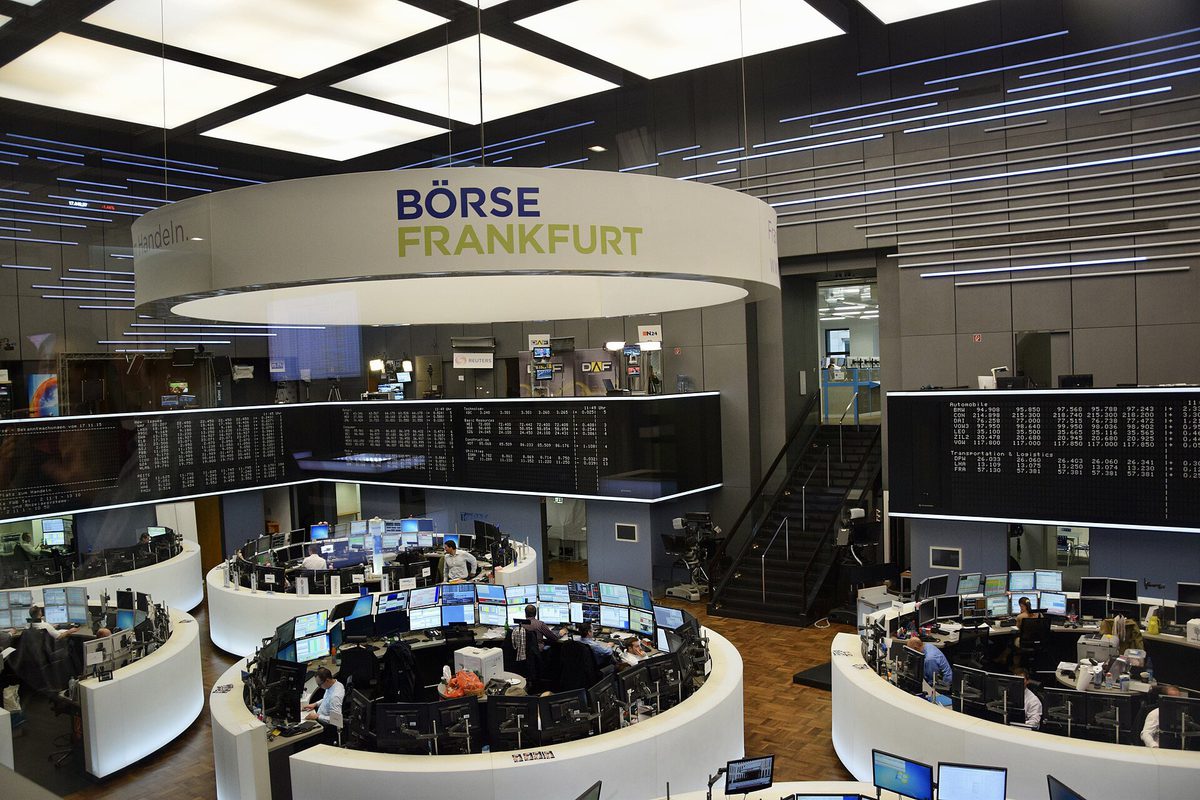
The S&P 500 Granger-causes the DAX with \(F = 94.6\) and the BET with \(F = 37.8\), both with p-values below 0.001. The reverse effects are much weaker: DAX → S&P 500 has \(F = 6.9\), BET → S&P 500 \(F = 1.0\) with p = 0.416. The coefficient of yesterday's S&P 500 return is 0.218 in the BET equation, with a standard error of 0.018, and 0.346 in the DAX equation. The photograph shows the trading floor of the Frankfurt Stock Exchange, where the DAX is traded.
Granger causality runs strongly and essentially in one direction, from the S&P 500 to the DAX and the BET. A return of 1% on the S&P 500 yesterday adds about 0.218% to the BET today, given the other lags. The BET does not Granger-cause the S&P 500 (p = 0.416): the small Bucharest market carries no information for New York.
The cause is the closing hours, non-synchronous trading, not a slow reaction of European markets. New York keeps trading after Europe closes, so "yesterday's" S&P 500 return happened partly while Europe was closed, and European prices reflect it only at the next opening. On weekly data, where the closing-time mismatch is small relative to the length of the period, the effect is much weaker, as Seminar 6 shows.
The regularity does not give a sure profit. The S&P 500 return of the previous evening is known before Bucharest opens, but prices adjust at the opening: an investor who buys at the opening price already pays the adjusted price. Granger causality in closing prices is a property of how the prices are recorded, not a source of riskless profit.
In brief
Strong one-way causality from the S&P 500 to the DAX and the BET: a 1% S&P return yesterday adds about 0.218% to the BET today
the BET does not Granger-cause the S&P 500 (p = 0.416)
Cause: the closing times (non-synchronous trading), not a slow market
New York keeps trading after Europe closes; “yesterday's” S&P return partly happened while Europe was closed
on weekly data the effect is much weaker (Seminar 6, B2)
Can you trade on it? You would buy at the Bucharest open, after prices have already adjusted: Granger causality in closing prices is not a free profit
Limitations of Granger causality: omitted variables
Granger causality depends on the information set. Adding or removing a variable can create or destroy it, as Lütkepohl (1982) showed. The typical mechanism is a common factor \(z\) that affects \(x\) earlier than \(y\): in a model without \(z\), the past of \(x\) is a proxy for the past of \(z\), so \(x\) appears to cause \(y\).
The simulation of the next slide makes the mechanism exact. The system is \(z_t = 0.5z_{t-1} + e_t\),\(x_t = 0.8z_{t-1} + u_t\) and \(y_t = 0.8z_{t-2} + v_t\), where \(e_t\),\(u_t\) and \(v_t\) are independent white noises with the standard Normal distribution. The variable \(x\) never appears in the equation of \(y\). But \(x_{t-1} = 0.8z_{t-2} + u_{t-1}\) is a noisy measurement of \(z_{t-2}\), which determines \(y_t\), so in a model without \(z\) the lag of \(x\) predicts \(y\).
An everyday example is ice-cream sales and drownings. In a bivariate model, ice-cream sales Granger-cause drownings, because both rise in summer; temperature, the omitted factor, explains both.
In brief
Granger causality is relative to the information set: adding or removing a variable can create or destroy it Lütkepohl (1982)
a common driver \(z\) that affects \(x\) earlier than \(y\) makes \(x\) look like a cause of \(y\)
Question for the room Set the effect of z on y to 0. What rejection rate does the VAR without z have at T = 500?
Answer
5.6%, close to the nominal 5% (between 4.5% and 5.6% for all sample sizes), against 100% with the effect 0.8 and 100% with 0.4. x looks like a cause of y only because xt−1 is a noisy measure of zt−2, which drives yt. The lag order matters too: with p = 1 even the VAR with z rejects in 76%–100% of the cases, because one lag of z does not contain zt−2, and xt−1 stands in for it.
The chart reports the result of 1,000 simulations of the system of the previous slide for each sample size \(T = 50, 100, 200\) and 500. In each simulation, the \(F\) test of "\(x\) does not Granger-cause \(y\)" is run at the 5% level in a VAR(2), once in the bivariate VAR of \(x\) and \(y\) (red bars, \(z\) omitted) and once in the trivariate VAR of \(x\),\(y\) and \(z\) (blue bars). The height of a bar is the rejection rate in percent; the dashed line marks the nominal size of 5%.
Since \(x\) never helps to forecast \(y\) once \(z\) is known, a correct test should reject in about 5% of the samples. The red bars show what happens when the test is run in the wrong information set.
In brief
1 000 simulations per sample size of the system of the previous slide; \(F\) test of “\(x\) does not Granger-cause \(y\)” at 5% in a VAR(2), with and without \(z\)
Without \(z\), the test rejects in 80% of the samples for \(T = 50\) and in 100% for \(T = 200\): it almost always finds a "cause". More data make things worse, not better: the test becomes ever more certain of a wrong conclusion, because the predictive link between \(x\) and \(y\) in the bivariate system is real; it is the interpretation that is wrong.
With \(z\) in the VAR, the rejection rate is between 4.3% and 5.2% across the four sample sizes, close to the nominal 5%: the test behaves as it should. Granger causality is a property of the chosen system, not of the world.
The Romanian data show the same dependence on a smaller scale. Inflation → GDP growth has p = 0.059 in the three-variable VAR and 0.173 in the bivariate VAR of inflation and GDP growth: the evidence changes when ROBOR is added or removed.
In brief
Without \(z\), the test rejects in 80% of samples with \(T = 50\) and 100% with \(T = 200\): almost always a “cause”
more data makes it worse: the test becomes more sure of a wrong conclusion
With \(z\) in the VAR, the rejection rate is 4.3%–5.2%, close to the nominal 5%
Granger causality is a property of the chosen system, not of the world
Romanian example: inflation \(\to\) GDP growth has p = 0.059 in the three-variable VAR and 0.173 in the bivariate one
Limitations of Granger causality: instantaneous causality
Granger tests use only lags. Effects within the same period are not in the coefficient matrices but in the correlation of the shocks, \(\bSigma\). There is instantaneous causality between \(x\) and \(y\) when \(\Cov(\varepsilon_{xt}, \varepsilon_{yt}) \ne 0\), which is tested with a Wald test on the off-diagonal elements of \(\bSigma\).
Instantaneous causality has no direction. A correlation of the shocks within a quarter says that \(x\) and \(y\) were surprised together, but the data cannot say whether \(x\) moved \(y\) or \(y\) moved \(x\) during the quarter. In the Romanian VAR, the ROBOR shocks are instantaneously correlated with the other shocks, with a p-value of 0.041, and the correlation of the inflation and ROBOR residuals is 0.25.
With quarterly data, many genuine effects happen within the quarter: a central bank can react to an inflation release within weeks. A VAR in which nothing is Granger-significant can therefore still contain strong links, all of them in \(\bSigma\). The section on impulse responses shows how these contemporaneous links are given a direction, and at what price.
In brief
Granger tests only use lags; effects within the same period are hidden in the correlation of the shocks \(\bSigma\)
instantaneous causality between \(x\) and \(y\): \(\Cov(\varepsilon_{xt}, \varepsilon_{yt}) \ne 0\); tested by a Wald test on the off-diagonal elements of \(\bSigma\)
It has no direction: the data cannot tell whether \(x\) moved \(y\) or \(y\) moved \(x\) within the quarter
Romania: ROBOR shocks are instantaneously correlated with the others (p = 0.041); the residual correlation of inflation and ROBOR is 0.25
With quarterly data, many true effects happen within the quarter: a VAR in which nothing is Granger-significant can still have strong links (Section 7)
Limitations of Granger causality: trends, expectations and the meaning of "cause"
The \(F\) and Wald tests have their usual distributions only for stationary variables. For integrated series, \(I(1)\),Sims, Stock and Watson (1990) showed that these statistics can have nonstandard distributions, so the usual critical values are wrong. Two remedies are common. If the series are not cointegrated, the test is run on their differences. Alternatively, Toda and Yamamoto (1995) proposed estimating a VAR(\(p + d_{\max}\)) in levels, where \(d_{\max}\) is the maximum order of integration of the series, usually 1, and testing only the first \(p\) lags; the extra lags are estimated but not tested, and they restore the standard \(\chi^2\) distribution of the Wald statistic. Cointegrated series require a VECM, the subject of Chapter 7.
Expectations create a second problem. Forward-looking prices move before the events they anticipate. Stock prices Granger-cause GDP, because investors price expected profits, and weather forecasts "Granger-cause" rain; neither is a cause in the ordinary sense. The forecast precedes the event because it is a forecast.
The correct way to report a significant result is therefore: "\(x\) helps to forecast \(y\), given these variables and this sample". The phrase "\(x\) causes \(y\)" claims more than the test can deliver.
In brief
Non-stationary variables: with \(I(1)\) series the \(F\) and Wald tests do not have their usual distributions Sims, Stock and Watson (1990)
remedies: test on differences (if there is no cointegration), or the Toda–Yamamoto approach Toda and Yamamoto (1995): estimate a VAR\((p + d_{\max})\) in levels and test only the first \(p\) lags
\(d_{\max}\): the highest order of integration of the series (usually 1); the extra lags are estimated but not tested
\(x\) Granger-causes \(y\) when the lags of \(x\) improve the forecast of \(y\); the test is an \(F\) or Wald test that the coefficients of those lags are zero. In the Romanian VAR, GDP growth and inflation Granger-cause ROBOR; on the markets, the S&P 500 Granger-causes the DAX and the BET, because of the time zones.
The pitfalls are omitted variables, which can create spurious causality; instantaneous effects, which the test does not see; nonstationarity, which invalidates the usual distributions; and expectations, which make forecasts precede events. Granger causality means predictability, not causation.
In brief
\(x \to y\) (Granger): the lags of \(x\) improve the forecast of \(y\); \(F\) or Wald test of zero restrictions
Romania: GDP growth and inflation \(\to\) ROBOR; markets: S&P 500 \(\to\) DAX, BET (time zones)
Granger causality is predictability, not causation
Section summary
Granger causality is a precise and testable concept, but a narrow one: it says whether the past of one variable improves the forecasts of another within a given system. In the Romanian VAR the information flows towards the interest rate, and on the markets from New York to Europe. The simulation showed how an omitted variable can produce a confident and wrong result. The next section moves from whether a variable helps to forecast another to how much and for how long it moves it.
Impulse responses
An impulse response traces how all variables of a VAR move over time after a single shock. This section defines impulse responses through the moving-average representation, explains why the correlation of the shocks forces an orthogonalisation, and introduces the Cholesky decomposition, in which the ordering of the variables is an identifying assumption. It applies the method to the Romanian VAR, shows how much the ordering matters, and introduces generalised impulse responses, which do not depend on the ordering, with an application to stock markets.
The impulse response function (IRF) is the path of \(Y_{j,t+h}\), for \(h = 0, 1, 2, \dots\), after a single shock in variable \(k\) at time \(t\), with all other shocks set to zero. From the moving-average representation (6.5), the response to a unit change in \(\varepsilon_{kt}\) is the column \(k\) of \(\bPhi_h\): element \((j, k)\) is the response of variable \(j\) after \(h\) periods.
The difficulty is that the shocks are correlated: \(\bSigma\) is not diagonal. "A shock to inflation with no shock to ROBOR" is an experiment the data rarely show, because in the Romanian VAR the two shocks usually come together, with correlation 0.25. A response to \(\varepsilon_{\pi}\) alone describes a combination of events that is atypical, and the responses to the different shocks overlap.
The solution is to rewrite the shocks as \(\bepsilon_t = \mathbf{P}\mathbf{u}_t\), where \(\mathbf{u}_t\) are uncorrelated shocks with unit variance and \(\mathbf{P}\) is a \(K \times K\) matrix with \(\bSigma = \mathbf{P}\mathbf{P}'\). The orthogonalised impulse responses are then
\[\boldsymbol{\Theta}_h = \bPhi_h\mathbf{P},\]
(6.9)
whose element \((j, k)\) is the response of \(Y_j\) after \(h\) periods to a shock \(u_k\) of one standard deviation. Since the \(u_k\) are uncorrelated, a shock to one of them while the others stay at zero is a meaningful experiment.
In brief
Impulse response function (IRF): the path of \(Y_{j,t+h}\), \(h = 0, 1, 2, \dots\), after a one-time shock to variable \(k\) at time \(t\)
from the moving-average form: the response to a unit change in \(\varepsilon_{kt}\) is the column \(k\) of \(\bPhi_h\)
Problem: the shocks are correlated (\(\bSigma\) not diagonal)
“a shock to inflation with no shock to ROBOR” is an experiment that the data rarely show: the two shocks usually come together (correlation 0.25)
Solution: rewrite the shocks as \(\bepsilon_t = \mathbf{P}\mathbf{u}_t\), with \(\mathbf{u}_t\) uncorrelated, unit variance: \(\bSigma = \mathbf{P}\mathbf{P}'\)
the orthogonalised IRF: \(\boldsymbol{\Theta}_h = \bPhi_h\mathbf{P}\); element \((j, k)\): the response of \(Y_j\) to a one-standard-deviation shock \(u_k\)
\(\mathbf{P}\): a \(K \times K\) matrix that turns the uncorrelated shocks \(\mathbf{u}_t\) into the observed shocks \(\bepsilon_t\)
Many matrices \(\mathbf{P}\) satisfy \(\bSigma = \mathbf{P}\mathbf{P}'\). The Cholesky decomposition picks the unique one that is lower triangular with a positive diagonal. For \(\bSigma\) with variances 1 and covariance 0.5, \(p_{11} = 1\),\(p_{21} = 0.5/1 = 0.5\) and \(p_{22} = \sqrt{1 - 0.25} = 0.866\), so \(\mathbf{P}\) has rows \((1.000, 0.000)\) and \((0.500, 0.866)\).
The triangular form gives a recursive structure: \(\varepsilon_{1t} = p_{11}u_{1t}\) and \(\varepsilon_{2t} = p_{21}u_{1t} + p_{22}u_{2t}\). The first variable is not moved by \(u_2\) in the same period, while the second reacts immediately to both shocks. The whole correlation between \(\varepsilon_1\) and \(\varepsilon_2\) is attributed to the shock of the variable ordered first.
The ordering therefore matters. With \(y_2\) first, the Cholesky factor, written in the original order, has rows \((0.866, 0.500)\) and \((0.000, 1.000)\): it is upper triangular, and now \(u_2\) carries the common part. The rule is to order the variables from the slowest, which does not react within the period to the others, to the fastest. For Romania the ordering is GDP growth, inflation, ROBOR: output and prices adjust slowly, while a market interest rate can respond within the quarter to news about both.
In brief
Cholesky: the unique lower triangular \(\mathbf{P}\) with positive diagonal such that \(\bSigma = \mathbf{P}\mathbf{P}'\)
the first variable is not moved by \(u_2\) in the same period; the second reacts to both at once
the whole correlation is attributed to the variable ordered first
The ordering matters: with \(y_2\) first, \(\mathbf{P} = \begin{pmatrix} 0.866 & 0.500 \\ 0.000 & 1.000 \end{pmatrix}\) (upper triangular in the original order)
rule: order from the slowest variable (does not react within the period) to the fastest; Romania: GDP growth, inflation, ROBOR
For the VAR(1) of the worked example, with the ordering \((y_1, y_2)\), the impact responses are \(\boldsymbol{\Theta}_0 = \mathbf{P}\), with rows \((1.000, 0.000)\) and \((0.500, 0.866)\). A shock \(u_1 = 1\) immediately moves \(y_1\) by 1 and \(y_2\) by 0.500, through the correlation of the shocks; a shock \(u_2 = 1\) moves only \(y_2\), by 0.866.
One period later, \(\boldsymbol{\Theta}_1 = \bA\mathbf{P}\), with rows \((0.600, 0.173)\) and \((0.500, 0.346)\). The response of \(y_2\) to \(u_1\) is 0.500, computed as \(0.3 \cdot 1 + 0.4 \cdot 0.5\): the direct effect \(a_{21}\) of last period's \(y_1\), plus the persistence \(a_{22}\) of \(y_2\)'s own impact response. Later horizons follow from \(\boldsymbol{\Theta}_h = \bA^h\mathbf{P}\).
When a VAR is written in growth rates, as is GDP growth in the Romanian VAR, the effect on the level is the cumulative response \(\sum_{s \le h}\boldsymbol{\Theta}_s\): a series of growth effects adds up to a permanent change in the level.
In brief
VAR(1) of Section 2, order \((y_1, y_2)\): \(\boldsymbol{\Theta}_0 = \mathbf{P} = \begin{pmatrix} 1.000 & 0.000 \\ 0.500 & 0.866 \end{pmatrix}\)
a shock \(u_1 = 1\) moves \(y_1\) by 1 and \(y_2\) by 0.500 at once; \(u_2 = 1\) moves only \(y_2\), by 0.866
One period later: \(\boldsymbol{\Theta}_1 = \bA\mathbf{P} = \begin{pmatrix} 0.600 & 0.173 \\ 0.500 & 0.346 \end{pmatrix}\)
\(y_2\) responds to \(u_1\) by 0.500: \(0.3 \cdot 1 + 0.4 \cdot 0.5\), the direct effect \(a_{21}\) plus its own persistence
The cumulative response \(\sum_{s \le h}\boldsymbol{\Theta}_s\) gives the effect on the level when the VAR is in growth rates
Question for the room Put ROBOR first (order i, g, π). What is the response of ROBOR to the inflation shock on impact and after 4 quarters?
Answer
0 on impact, by construction, and 0.64 pp after 4 quarters, against 0.23 and 0.82 pp in the lecture’s ordering; the band excludes zero at 9 of the 13 horizons, against 11. With ROBOR first, the common part of the two shocks (residual correlation 0.25) is assigned to ROBOR. The qualitative conclusion stays: ROBOR rises after an inflation shock and stays higher for years (0.38 pp after 12 quarters).
The chart is a 3 × 3 grid of orthogonalised impulse responses of the Romanian VAR(2), for horizons 0 to 12 quarters. Each row is a responding variable and each column a shock of one standard deviation; the panel "ROBOR 3M ← inflation", for instance, shows how ROBOR responds to an inflation shock. The vertical axes are in percentage points. The Cholesky ordering is \(g, \pi, i\).
The shaded areas are 90% bands from a residual bootstrap with 500 replications, following Kilian (1998): the VAR is re-estimated on artificial samples built by resampling the residuals, and the bands contain the middle 90% of the resulting responses. A response whose band excludes zero at a horizon is distinguishable from zero there. The bootstrap is preferred here because the residuals are far from Normal.
In brief
Row: responding variable; column: shock of one standard deviation; Cholesky order \(g, \pi, i\); 90% bands from a residual bootstrap (500 replications) Kilian (1998)
An inflation shock, of 1.08 percentage points (pp) on impact, raises ROBOR immediately by 0.23 pp, by up to 0.82 pp after 4 quarters, and still by 0.44 pp after 3 years. The band excludes zero at 11 of the 13 horizons, which makes this the clearest result of the VAR. It is the dynamic counterpart of the Granger test inflation → ROBOR.
A ROBOR shock reduces GDP growth by 0.61 pp in the following quarter, and then the effect disappears. Inflation, however, rises after a ROBOR shock, by up to 0.16 pp, a response not significant but with the wrong sign: a monetary tightening should lower inflation. This is the price puzzle documented by Sims (1992). A likely reason is that the interest rate rises when the central bank anticipates inflation; the information it uses, such as the exchange rate or energy prices, is missing from the VAR, so the anticipated inflation appears to follow the "shock".
Inflation shocks are persistent: the response of inflation to its own shock is 1.18 pp after one year and 0.24 pp after three. The slow fading reflects the largest eigenvalue of the model, 0.869.
In brief
An inflation shock (1.08 pp on impact) raises ROBOR by 0.23 pp at once and by up to 0.82 pp after 4 quarters; still 0.44 pp after 3 years
the band excludes zero for 11 of the 13 horizons: the clearest result of the VAR
A ROBOR shock lowers GDP growth by 0.61 pp the next quarter, then the effect vanishes
but inflation rises after a ROBOR shock (up to 0.16 pp, not significant): the “price puzzle” Sims (1992)
a likely reason: the rate rises when the central bank expects inflation; information omitted from the VAR (exchange rate, energy prices) shows up as a “shock”
Inflation shocks themselves are persistent: 1.18 pp after a year, 0.24 pp after three
Question for the room Move to p = 1. Does inflation still rise after a ROBOR shock (the “price puzzle”) when inflation comes before ROBOR?
Answer
No: the largest response is 0.00 pp, on impact (zero by the ordering), and the response is negative afterwards; with p = 2 it rose to 0.16 pp. With ROBOR first, the impact is 0.29 pp in the VAR(1) as well, because the ordering assigns the common part of the shocks to ROBOR. The “puzzle” depends here on both the ordering and the number of lags: a result that changes with p and with the ordering is fragile.
The chart compares, for the same VAR(2), the two responses that involve inflation and ROBOR under three schemes. The solid blue line uses the ordering \(g, \pi, i\), with inflation before ROBOR; the dashed red line uses \(g, i, \pi\), with ROBOR before inflation; the dotted green line shows the generalised responses of Pesaran and Shin (1998), which do not depend on the ordering. The left panel is the response of ROBOR to an inflation shock, the right panel the response of inflation to a ROBOR shock, both in percentage points for horizons 0 to 12 quarters.
Only the position of inflation and ROBOR relative to each other changes; GDP growth stays first. The differences between the lines therefore come entirely from how the correlation of 0.25 between the inflation and ROBOR shocks is attributed.
In brief
Same VAR(2), two Cholesky orderings (inflation before ROBOR, ROBOR before inflation) and the generalised responses of Pesaran and Shin (1998), which do not depend on the order
The response of ROBOR to an inflation shock peaks at 0.82 pp with inflation first, against 0.64 pp with ROBOR first. With ROBOR first, the impact response is zero by construction, since a variable ordered before inflation cannot react to the inflation shock within the period. The shape is the same, but the size depends on the ordering.
The response of inflation to a ROBOR shock changes much more: 0.16 pp at its peak with inflation first, against 0.53 pp with ROBOR first, with 0.29 pp already on impact. The second ordering attributes the common part of the two shocks to ROBOR, so a ROBOR shock now carries part of what was an inflation surprise, and the price puzzle grows.
The ordering is an assumption about which variable reacts within the quarter. It must be stated and justified, and results that change with it are fragile. Here the main finding, a persistent rise of ROBOR after an inflation shock, survives both orderings; the response of inflation to ROBOR does not.
In brief
ROBOR after an inflation shock: peak 0.82 pp (inflation first) against 0.64 pp (ROBOR first)
with ROBOR first, the impact response is zero by construction
Inflation after a ROBOR shock: 0.16 pp against 0.53 pp, with 0.29 pp already on impact
the second ordering assigns the common part of the two shocks (correlation 0.25) to ROBOR, so the “price puzzle” gets larger
The ordering is an assumption about which variable reacts within the quarter; it must be stated and defended, and results that change with it are fragile
The generalised impulse response of Pesaran and Shin (1998), building on Koop, Pesaran and Potter (1996), avoids the choice of an ordering. It gives variable \(k\) a shock of one standard deviation and lets the other shocks move as they typically move with it, according to their historical correlations:
where \(\mathbf{e}_k\) is the column \(k\) of the identity matrix and \(\sigma_{kk}\) the variance of shock \(k\). The term \(\bSigma\mathbf{e}_k/\sqrt{\sigma_{kk}}\) is the expected impact vector given a one-standard-deviation shock to \(\varepsilon_k\).
No ordering is needed, and for the variable ordered first, the generalised response coincides with the Cholesky response, since in both the first shock carries all of its correlation with the others. The price is that generalised shocks are not orthogonal: the responses to different shocks overlap, because each one includes the common movements, and they cannot be added up or used to split the variance into shares.
Generalised responses are useful for markets, where no ordering is natural because prices react to each other within seconds. They describe typical joint movements, not structural shocks with an economic interpretation.
\(\boldsymbol{\psi}_k(h) = \bPhi_h\bSigma\mathbf{e}_k/\sqrt{\sigma_{kk}}\); \(\mathbf{e}_k\): column \(k\) of the identity matrix; \(\sigma_{kk}\): the variance of shock \(k\)
Properties
no ordering is needed; for the variable ordered first, it equals the Cholesky response
the shocks are not orthogonal: the responses to different shocks overlap and cannot be added up
Useful for markets, where no ordering is natural; it describes typical co-movements, not structural shocks
Question for the room Start the sample in 2015. What does the generalised response of the BET the day after an S&P 500 shock become?
Answer
0.11%, against 0.24% over 2000–2026; the same-day response stays 0.32%. For the DAX the response falls from 0.85% to 0.68% on the same day and from 0.24% to 0.16% the next day. The next-day part, which comes from the different closing times, is about half as large after 2015.
The chart shows the responses of the DAX (left) and the BET (right) to a one-standard-deviation shock in the S&P 500, 1.21%, in a VAR(4) of daily returns, for days 0 to 5, in percent. Three schemes are compared: generalised responses (green), Cholesky with the S&P 500 first (blue), and Cholesky in the order of the closing times, BET, DAX, S&P 500, with the S&P 500 last (red).
Day 0 is the day of the S&P 500 shock. The two Cholesky orderings make opposite assumptions about that day: with the S&P 500 first, New York's news moves Europe on the same calendar day; with the S&P 500 last, it cannot, because Europe closed before New York.
In brief
VAR(4) of daily S&P 500, DAX and BET returns; S&P shock of one standard deviation (1.21%); generalised responses, Cholesky with the S&P 500 first, and Cholesky in the order of the closing times (BET, DAX, S&P 500)
The generalised responses are 0.85% for the DAX on the same day and 0.24% on the next day; for the BET, 0.32% and 0.24%. They are identical to the Cholesky responses with the S&P 500 first, as theory says for the variable ordered first.
With the S&P 500 last, the order in which the exchanges close, the same-day response is zero by assumption, and the next-day responses are 0.32% for the DAX and 0.20% for the BET. In this ordering the same-day correlation of the shocks, 0.63 between the S&P 500 and the DAX, is attributed to Europe: a common movement on the same calendar day is read as Europe moving New York, not the other way round.
In both versions, the effect has disappeared after two days: from day 2 onwards all responses are close to zero. The markets incorporate the information from New York at their next opening and then no longer react to it.
In brief
Generalised: DAX 0.85% on the same day and 0.24% the next; BET 0.32% and 0.24%
identical to the Cholesky responses with the S&P 500 first, as the theory says
With the S&P 500 last (it closes last), the same-day response is zero by assumption and the next-day responses are 0.32% (DAX) and 0.20% (BET)
the same-day correlation (0.63 with the DAX) is attributed to Europe in this order
Either way, the effect is over after two days: markets absorb the news quickly
Impulse responses are the columns of \(\bPhi_h\); the orthogonalised responses are \(\boldsymbol{\Theta}_h = \bPhi_h\mathbf{P}\), with \(\bSigma = \mathbf{P}\mathbf{P}'\). The Cholesky factor imposes a recursive ordering, which is an assumption and can change the results.
In the Romanian VAR, ROBOR rises for years after an inflation shock, and the response of inflation to a ROBOR shock shows the price puzzle. Generalised responses do not depend on the ordering but are not additive. Bands from a bootstrap provide the inference.
Cholesky = recursive ordering; the ordering is an assumption and can change the results
Romania: ROBOR rises for years after an inflation shock; a “price puzzle” appears
Generalised IRF: order-free, but not additive; bootstrap bands for inference
Section summary
Impulse responses turn the estimated VAR into statements about dynamics: how much and for how long one variable moves after a shock to another. Their weak point is the identification of the shocks, which the Cholesky ordering settles by assumption; checking alternative orderings and generalised responses shows which results depend on it. The next section uses the same orthogonal shocks to divide the forecast uncertainty of each variable among the shocks.
Forecast error variance decomposition
The forecast error variance decomposition answers a different question from impulse responses: which shocks account for the uncertainty in forecasting each variable? This section derives the decomposition, applies it to the Romanian VAR, and presents the spillover index of Diebold and Yilmaz, which turns the decomposition into a measure of how connected markets are, computed for the S&P 500, the DAX and the BET.
The error of the forecast \(h\) steps ahead is the sum of the shocks that occur between \(t\) and \(t + h\), weighted by the moving-average matrices: \(\bY_{t+h} - \hat\bY_{t+h|t} = \sum_{s=0}^{h-1}\bPhi_s\bepsilon_{t+h-s} = \sum_{s=0}^{h-1}\boldsymbol{\Theta}_s\mathbf{u}_{t+h-s}\), where \(\hat\bY_{t+h|t}\) is the forecast of \(\bY_{t+h}\) made at time \(t\). Since the orthogonal shocks \(u_k\) are uncorrelated with unit variance, the variance of each element of this error splits into \(K\) parts, one per shock.
The forecast error variance decomposition (FEVD) gives the share of shock \(k\) in the \(h\)-step forecast error variance of \(Y_j\):
where \(\theta_{jk,s}\) is the element \((j, k)\) of \(\boldsymbol{\Theta}_s\). Each row sums to 100% across the shocks. The decomposition depends on the Cholesky ordering, and at \(h = 1\) the first variable is explained 100% by its own shock, because no other shock moves it on impact.
For the VAR(1) of the worked example, at \(h = 2\) the forecast error variance of \(y_2\) is 1.37. The shock \(u_1\) contributes the squares of its two responses, the impact \(p_{21} = 0.5\) and the next-period response 0.500, so its share is \((0.5^2 + 0.5^2)/1.37 = 36.5\%\); the remaining 63.5% comes from \(u_2\).
the orthogonal shocks \(u_k\) are uncorrelated, so the variance splits into \(K\) parts
FEVD: \(\omega_{jk}(h) = \dfrac{\sum_{s=0}^{h-1}\theta_{jk,s}^2}{\sum_{s=0}^{h-1}\sum_{m=1}^{K}\theta_{jm,s}^2}\), the share of shock \(k\) in the \(h\)-step error variance of \(Y_j\)
\(\theta_{jk,s}\): element \((j, k)\) of \(\boldsymbol{\Theta}_s\); \(\hat\bY_{t+h|t}\): the forecast of \(\bY_{t+h}\) made at \(t\)
each row sums to 100%; it depends on the Cholesky ordering; at \(h = 1\) the first variable is explained 100% by its own shock
Example (VAR(1) of Section 2), \(h = 2\): the variance of the error of \(y_2\) is 1.37; shock \(u_1\) explains 36.5%
\((0.5^2 + 0.5^2)/1.37\): the impact \(p_{21} = 0.5\) and the next-period response 0.500
Question for the room Choose the order i, π, g (ROBOR first). How much of the 12-quarter forecast error variance of ROBOR do inflation shocks explain?
Answer
27%, against 53% in the lecture’s ordering; ROBOR’s own shocks explain 63% instead of 37%. At one quarter ROBOR is explained 100% by its own shock, by construction. The conclusion that in the long run the interest rate is driven mainly by inflation therefore rests on the assumption that ROBOR reacts to inflation within the quarter, not the other way round.
The chart shows the FEVD of the Romanian VAR(2), one panel per variable, for horizons of 1 to 12 quarters, with the Cholesky ordering \(g, \pi, i\). Each bar is split into the shares of the three orthogonal shocks: GDP growth (green), inflation (red) and ROBOR 3M (blue). The bars all reach 100%.
The three panels show three different patterns. GDP growth and inflation are dominated at every horizon by their own shocks, while the composition of the ROBOR bars changes with the horizon: blue dominates at short horizons, red at long ones.
In brief
Share of each orthogonal shock in the forecast error variance, horizons 1–12 quarters, Cholesky order \(g, \pi, i\)
For ROBOR, its own shocks explain 92% of the forecast error variance at one quarter but only 37% after three years; at that horizon, inflation shocks explain 53% and GDP growth shocks 10%. In the long run, the uncertainty about the interest rate comes mainly from inflation: to forecast ROBOR three years ahead, one must above all forecast inflation.
Inflation is explained 97% by its own shocks even after 12 quarters, and GDP growth 90% by its own shocks. In this small VAR, inflation is driven by factors outside the model, such as energy and food prices, the exchange rate and taxes, which appear as inflation's own shocks. A larger VAR could attribute part of this variance to those factors.
The FEVD and the Granger tests agree: information flows from inflation and output to the interest rate, and hardly in the other direction.
In brief
ROBOR: own shocks explain 92% at one quarter, but only 37% after three years; inflation shocks explain 53%, GDP shocks 10%
in the long run, the interest rate is mostly driven by inflation
Inflation: 97% own shocks even after 12 quarters; GDP growth: 90% own shocks
in this small VAR, inflation is driven by forces outside the model (energy, food, exchange rate, taxes)
FEVD and Granger tests agree: the information flows from inflation and output to the interest rate
Diebold and Yilmaz asked how much of the forecast uncertainty of one market comes from shocks in other markets, and how this changes over time. Diebold and Yilmaz (2009) used a Cholesky FEVD of weekly returns of 19 stock markets. Diebold and Yilmaz (2012) replaced it with the generalised FEVD, built from generalised impulse responses, which removes the dependence on the ordering.
The spillover index is the average share of the forecast error variance that comes from the other markets:
where \(\tilde\omega_{jk}\) is the generalised FEVD, rescaled so that each row sums to 1; the rescaling is needed because generalised shares do not add up to 1 by themselves. The specification of Diebold and Yilmaz (2012) is a VAR(4), a horizon \(H = 10\) days, and rolling windows of 200 days, so that the index can be tracked over time.
Their main result is that spillovers rise sharply in crises: markets become more connected exactly when diversification is most needed. The next slides compute the index for the S&P 500, the DAX and the BET.
In brief
Question: how much of the forecast uncertainty of one market comes from shocks in other markets, and how does it change over time?
Spillover index: \(S(H) = \frac{100}{K}\sum_{j \ne k}\tilde\omega_{jk}(H)\), the average share of other markets' shocks
\(\tilde\omega_{jk}\): generalised FEVD rescaled so that each row sums to 1; the specification of Diebold and Yilmaz (2012): VAR(4), \(H = 10\) days, rolling 200-day windows
Finding: spillovers rise sharply in crises; markets become more connected exactly when diversification is most needed
next: the index for the S&P 500, the DAX and the BET
The table is a generalised FEVD at a horizon of 10 days, estimated on the full sample 2000–2026. Row \(j\) gives the shares of the 10-day forecast error variance of market \(j\) due to shocks in each market, in percent; each row sums to 100. The diagonal is the share of a market's own shocks; the column "from others" is the row sum of the off-diagonal elements, and the row "to others" is the column sum of the off-diagonal elements, what a market transmits to the others.
The S&P 500 receives 27.1% from the DAX, and the DAX 28.2% from the S&P 500: the two large markets are strongly connected in both directions. The BET receives 14.7% from the others and transmits only 9.1%: it is a small market and a net receiver. The total spillover index, the average of the "from others" column, is 26.4%.
In brief
To \(\leftarrow\) from (%)
S&P 500
DAX
BET
from others
S&P 500
69.2
27.1
3.7
30.8
DAX
28.2
66.4
5.4
33.6
BET
7.2
7.5
85.3
14.7
to others
35.4
34.6
9.1
index 26.4
Row \(j\): shares of the 10-day forecast error variance of market \(j\) due to shocks in each market (generalised FEVD, full sample 2000–2026)
The S&P 500 receives 27.1% from the DAX and the DAX 28.2% from the S&P 500; the BET receives 14.7% and gives only 9.1%: a small, net receiving market
Question for the room Widen the window to 500 days. What does the maximum of the index become, and when does it occur?
Answer
47.3%, on 22 September 2021, against 57.5% on 17 March 2020 with 200-day windows. A longer window mixes the crash of March 2020 with more calm days, so the peak is lower and comes later; the mean stays almost the same (29.1% against 29.0%). The size and date of the peaks depend on the window length: part of the jumps is mechanical.
The chart shows the total spillover index of the S&P 500, DAX and BET daily returns, computed from a generalised FEVD at 10 days of a VAR(4) estimated on rolling windows of 200 trading days. Each point uses the 200 days that end on that date; the dashed red line is the full-sample index, 26.4%, and the mean of the rolling index is 29.0%. Vertical lines mark four events: the failure of Lehman Brothers in 2008, the downgrade of the US credit rating in 2011, the COVID-19 crash in 2020 and the Russian invasion of Ukraine in 2022.
The index moves in steps: it jumps when a turbulent period enters the window and falls 200 days later when that period leaves it.
In brief
Total spillover index of S&P 500, DAX and BET daily returns: generalised FEVD at 10 days from a VAR(4), rolling windows of 200 trading days (29.0% on average)
The index rose from 28% in 2007 to 47% in 2008 Q4, after the failure of Lehman Brothers, and reached its maximum, 57.5%, on 17 March 2020, in the COVID-19 crash. It is the same pattern that Diebold and Yilmaz (2009) found for 19 markets: connectedness rises abruptly in crises and declines slowly.
The latest value is 22.7%, below the full-sample index of 26.4%. Part of the jumps is mechanical: a 200-day window that contains a crash is dominated by it for 200 days, so the index stays high until the crash leaves the window, which explains the flat plateaus after each event.
For a portfolio that includes the BET, the lesson is that diversification across these markets helps least when it is most needed: in a crisis, a larger share of each market's risk comes from shocks common to all.
In brief
From 28% in 2007 to 47% in 2008Q4 (after Lehman); maximum 57.5% on 17 March 2020, in the COVID-19 crash
The FEVD gives the share of each orthogonal shock in the forecast error variance at horizon \(h\); each row sums to 100%. In the Romanian VAR, ROBOR is driven by inflation at long horizons, while inflation is driven mainly by its own shocks.
The Diebold–Yilmaz spillover index is the total off-diagonal share of the generalised FEVD. For the S&P 500, DAX and BET, it peaks in crises, in 2008 and in 2020.
In brief
FEVD: share of each orthogonal shock in the \(h\)-step forecast error variance; rows sum to 100%
Romania: ROBOR is driven by inflation at long horizons; inflation mainly by its own shocks
Diebold–Yilmaz spillover index: the off-diagonal mass of the generalised FEVD
Spillovers among S&P 500, DAX and BET peak in crises (2008, 2020)
Section summary
The variance decomposition summarises the system by the sources of its forecast uncertainty. In the Romanian VAR, it confirms that inflation drives the interest rate at long horizons; across markets, it measures connectedness and shows how it rises in crises. The next section turns to the forecasts themselves.
Forecasting with a VAR
This section shows how point forecasts and forecast intervals are produced from a VAR, applies them to the Romanian VAR(2) for two years ahead, and asks whether the VAR forecasts better than univariate methods. The answer requires a pseudo out-of-sample evaluation, a comparison with simple benchmarks and a test of equal accuracy; it is given for Romania and for the United States.
Point forecasts are computed by recursion: \(\hat\bY_{T+h|T} = \bc + \bA_1\hat\bY_{T+h-1|T} + \dots + \bA_p\hat\bY_{T+h-p|T}\), where \(\hat\bY_{T+j|T} = \bY_{T+j}\) for \(j \le 0\), so observed values are used wherever they exist. Each step uses the forecasts of the previous steps in place of the unknown future values. For a stable VAR, the forecasts converge to the mean \(\boldsymbol{\mu}\) as \(h\) grows.
The covariance matrix of the \(h\)-step forecast error follows from the moving-average representation:
It grows with \(h\) and converges to the variance of the process, \(\bGamma(0)\): far ahead, the forecast is the mean, and its error has the variance of the series. The 95% interval for variable \(j\) is \(\hat Y_{j,T+h|T} \pm 1.96\sqrt{\sigma_{jj}(h)}\), where \(\sigma_{jj}(h)\) is the element \((j, j)\) of \(\bSigma(h)\). It assumes Normal shocks and ignores the uncertainty of the estimated parameters, so it is somewhat too narrow in small samples.
For the worked example, \(\bSigma(2) = \bSigma + \bA\bSigma\bA'\), with variances 1.39 for \(y_1\) and 1.37 for \(y_2\), against 1 for the one-step forecast. The logic is that of the ARMA forecasts of Chapter 2, with matrices in place of numbers.
In brief
Point forecasts by recursion: \(\hat\bY_{T+h|T} = \bc + \bA_1\hat\bY_{T+h-1|T} + \dots + \bA_p\hat\bY_{T+h-p|T}\), with \(\hat\bY_{T+j|T} = \bY_{T+j}\) for \(j \le 0\)
for a stable VAR they converge to the mean \(\boldsymbol{\mu}\) as \(h\) grows
Error covariance: \(\bSigma(h) = \sum_{s=0}^{h-1}\bPhi_s\bSigma\bPhi_s'\); it grows with \(h\) towards \(\bGamma(0)\)
95% interval for \(Y_j\): \(\hat Y_{j,T+h|T} \pm 1.96\sqrt{\sigma_{jj}(h)}\), \(\sigma_{jj}(h)\): element \((j, j)\) of \(\bSigma(h)\) (Normal shocks; parameter uncertainty ignored)
example (Section 2): \(\bSigma(2) = \bSigma + \bA\bSigma\bA'\), with variances 1.39 and 1.37
Same logic as the ARMA forecasts of Chapter 2, with matrices in place of numbers
Question for the room Move the origin to 2020Q4. Is the inflation realised in 2022Q4 inside the 95% interval of the 8-quarter forecast?
Answer
No: 13.2% realised, against a forecast of 2.4% and the interval [−2.3; 7.1]. The VAR estimated up to 2020 contains none of the energy-price shocks of 2021–2022, and the interval assumes Normal shocks with the past variance and ignores parameter uncertainty. With the origin 2019Q4, the inflation of 2021Q4 (6.4%) was still inside the interval ([−2.0; 7.7]).
The chart shows the data from 2019 to 2026 Q2 and the forecasts of the VAR(2) for 2026 Q3 – 2028 Q2, eight quarters, for GDP growth, inflation and ROBOR 3M. The solid lines are the data, the dashed lines the point forecasts and the shaded areas the 95% intervals.
The intervals widen with the horizon at different rates. The interval for GDP growth reaches its full width almost at once, because GDP growth has little persistence; the intervals for inflation and ROBOR widen steadily, because errors in persistent series accumulate.
In brief
Data until 2026Q2; forecasts 2026Q3–2028Q2 with 95% intervals
Inflation is forecast to fall from 9.1% in 2026 Q2 to 7.7% after one year and 6.3% after two, with a 95% interval of −0.1% to 12.7% at the two-year horizon. The forecasts move towards the mean of the VAR, 4.8% for both inflation and ROBOR, but slowly, because the largest eigenvalue is 0.869.
ROBOR is forecast at 6.4% after one year and 6.2% after two. GDP growth is forecast at about 0.5% per quarter, with an interval from −4.4% to 5.3%. The interval is wide because the extreme values of 2009 and 2020 raise the estimated residual standard deviation \(\hat\sigma_g\), and with it the width of every interval.
These are mechanical forecasts. The VAR knows nothing about the budget, energy prices or the decisions of the BNR; it extrapolates the average dynamics of 2005–2026. Its value is that of a transparent benchmark, against which judgemental forecasts can be compared and their departures explained.
In brief
Inflation: from 9.1% in 2026Q2 to 7.7% after a year and 6.3% after two (95%: \([-0.1, 12.7]\))
the forecasts move towards the VAR mean (inflation 4.8%, ROBOR 4.8%), slowly because the largest eigenvalue is 0.869
ROBOR: 6.4% after a year, 6.2% after two; GDP growth: 0.5% per quarter, with an interval \([-4.4, 5.3]\)
the GDP interval is wide because the 2009 and 2020 outliers inflate \(\hat\sigma_g\)
A mechanical forecast: it knows nothing of the budget, energy prices or BNR decisions; its value is as a transparent benchmark
A fair evaluation uses a pseudo out-of-sample design. At each forecast origin \(t\), the model is re-estimated only on data up to \(t\), the forecast for \(t + h\) is made, and the origin moves forward one period, with an expanding window. The forecasts are never evaluated on data that were used to estimate the model, the rule of Chapter 0.
The VAR is compared with two benchmarks: the random walk, which forecasts no change, and a univariate AR(\(p\)) for each variable, with \(p\) chosen by AIC. The question is not "is the VAR good?" but "do the other variables add anything to the series' own past?" Only the comparison with the AR model answers that.
Accuracy is measured by the root mean squared error (RMSE) relative to the random walk, so that a value below 1 means better than no change. The test of Diebold and Mariano (1995) checks whether two forecasts have equal accuracy. Its statistic, DM, is the mean difference of the squared errors of the two forecasts divided by its standard error, and it is approximately \(N(0, 1)\) under the null hypothesis of equal accuracy.
In brief
Pseudo out-of-sample: re-estimate on data up to \(t\) only, forecast \(t + h\), move \(t\) forward (expanding window)
never evaluate on the data used for estimation (Chapter 0)
Benchmarks: the random walk (no change) and a univariate AR\((p)\) for each variable, \(p\) by AIC
the question is not “is the VAR good?”, but “do the other variables add anything to the series' own past?”
Measures: RMSE relative to the random walk (below 1: better); the Diebold–Mariano test Diebold and Mariano (1995) for equal accuracy
DM statistic: the mean difference of squared errors divided by its standard error; approximately \(N(0, 1)\) under \(H_0\)
Question for the room Start the evaluation for Romania in 2021 (h = 1). Is the VAR still significantly less accurate than the AR for GDP growth?
Answer
Not at 5%: relative RMSE 1.06 for the VAR and 0.76 for the AR, but DM = 1.74, p = 0.082, on only 22 forecasts. The difference still favours the AR, and the VAR is now less accurate than even the random walk; with half the forecasts, the test no longer separates it from noise at 5%.
The chart reports the RMSE of the AR (ochre bars) and VAR (blue bars) forecasts, each divided by the RMSE of the random walk; the dashed line at 1 is the random walk. The left panel is Romania, with 46 forecasts per horizon from origins 2014 Q4 to 2026 Q1, for horizons \(h = 1\) and 4 quarters and each of \(g\),\(\pi\) and \(i\). The right panel is the US VAR of the Stock–Watson case study, with forecasts for 1985 Q1 – 2000 Q4, the evaluation period of Stock and Watson (2001), for horizons 2, 4 and 8 quarters and each of inflation \(\pi\), unemployment \(u\) and the federal funds rate \(R\).
A blue bar below the ochre bar means that the VAR beats the univariate AR; a bar above 1 means that the model is worse than forecasting no change.
In brief
Relative RMSE (model / random walk). Left: Romania, 46 forecasts per horizon, origins 2014Q4–2026Q1; right: the US VAR of Section 10, forecasts for 1985Q1–2000Q4, the evaluation period of Stock and Watson (2001)
For Romania at a horizon of one quarter, the VAR is less accurate than the AR for GDP growth: its relative RMSE is 0.85 against 0.75, and the Diebold–Mariano statistic is 2.59, with p-value 0.010. It is not better for inflation or ROBOR either. The VAR has 21 coefficients estimated on 38 to 84 quarters, depending on the origin, and the estimation error cancels the information brought by the other variables.
For the United States at a horizon of 8 quarters, the VAR is more accurate than the AR for unemployment, 0.70 against 0.85, and for the federal funds rate, 0.79 against 0.90. For inflation, neither model beats the random walk at this horizon and in this period: the relative RMSE of the VAR is 1.22.
VARs help when the sample is long and the links between the variables are strong, as in the US data with 25 years of estimation data and a clear policy reaction. In short and noisy samples, a simple AR is hard to beat.
In brief
Romania, one quarter ahead: the VAR loses to the AR for GDP growth (0.85 against 0.75; DM = 2.59, p = 0.010) and is no better for inflation or ROBOR
21 coefficients on 38 to 84 quarters: the estimation noise eats the information of the other variables
United States, 8 quarters ahead: the VAR beats the AR for unemployment (0.70 against 0.85) and the fed funds rate (0.79 against 0.90)
for inflation, nothing beats the random walk (1.22) at this horizon in this period
VARs help when the sample is long and the links are strong; in short, noisy samples a simple AR is hard to beat
Point forecasts are computed recursively, and the forecast error covariance is \(\sum_s\bPhi_s\bSigma\bPhi_s'\). Forecasts are evaluated out of sample, against the random walk and univariate AR models.
For Romania, the VAR brings no forecasting gain; for the United States in 1985–2000, it gains for unemployment and the interest rate.
In brief
Recursive point forecasts; error covariance \(\sum_s\bPhi_s\bSigma\bPhi_s'\)
Evaluate out of sample against the random walk and univariate AR models
Romania: no gain from the VAR; US 1985–2000: gains for unemployment and the interest rate
Section summary
A VAR produces joint forecasts with intervals by the same recursion as an ARMA model, and its forecasts revert to the mean at the speed set by the largest eigenvalue. Whether it forecasts better than univariate models is an empirical question, answered out of sample: often it does not, because estimating many coefficients costs more than the extra information is worth. The next section returns to the interpretation of the shocks.
Structural VARs and a landmark case study
The reduced-form VAR describes the data; a structural VAR gives its shocks an economic meaning, such as a monetary policy shock. This section shows how the two are related and why the step from one to the other always requires assumptions. It then re-estimates the VAR of Stock and Watson (2001) for the United States and closes with the legacy of the VAR approach.
where \(\mathbf{u}_t\) are uncorrelated structural shocks, \(\mathbf{d}\) is the vector of intercepts, \(\mathbf{B}_1, \dots, \mathbf{B}_p\) are the structural lag coefficients, and \(\mathbf{B}_0\) contains the contemporaneous effects, for example the reaction of the policy interest rate to this quarter's inflation. Multiplying by \(\mathbf{B}_0^{-1}\) gives the reduced form (6.2), with \(\bA_j = \mathbf{B}_0^{-1}\mathbf{B}_j\) and \(\bepsilon_t = \mathbf{B}_0^{-1}\mathbf{u}_t\): each reduced-form shock is a combination of structural shocks.
The data identify only the reduced form. The covariance matrix \(\bSigma\) has \(K(K+1)/2\) distinct elements, while \(\mathbf{B}_0^{-1}\) has \(K^2\) elements; with the structural shocks normalised to unit variance, \(K(K-1)/2\) further restrictions are needed to recover \(\mathbf{B}_0^{-1}\) from \(\bSigma\). The Cholesky decomposition sets \(\mathbf{B}_0^{-1} = \mathbf{P}\), lower triangular, with exactly \(K(K-1)/2\) zeros: this is the recursive SVAR of Sims (1980). Other schemes use long-run restrictions, sign restrictions or external instruments, beyond this course.
The general lesson is that the data identify the reduced form, and a structural interpretation always rests on assumptions that must be argued on economic grounds. The impulse responses of the Romanian VAR are structural only to the extent that the ordering GDP growth, inflation, ROBOR is a credible description of what reacts within a quarter.
\(\mathbf{d}\): constants; \(\mathbf{B}_1, \dots, \mathbf{B}_p\): structural lag coefficients; \(\mathbf{B}_0\): the contemporaneous effects (e.g. the policy rate reacts to this quarter's inflation)
multiplying by \(\mathbf{B}_0^{-1}\) gives the reduced form, with \(\bepsilon_t = \mathbf{B}_0^{-1}\mathbf{u}_t\)
Identification: \(\bSigma\) has \(K(K+1)/2\) distinct elements, \(\mathbf{B}_0^{-1}\) has \(K^2\); we need \(K(K-1)/2\) restrictions
Cholesky: \(\mathbf{B}_0^{-1} = \mathbf{P}\) lower triangular: exactly \(K(K-1)/2\) zeros; the recursive SVAR of Sims (1980)
other schemes: long-run restrictions, sign restrictions, external instruments (beyond this course)
The data identify the reduced form; the structural interpretation always rests on assumptions that must be argued with economics
Stock and Watson (2001), "Vector autoregressions", is a widely used survey of the method. Its example is a VAR in three US variables: inflation \(\pi_t\), the unemployment rate \(u_t\) and the federal funds rate \(R_t\). Inflation is \(\pi_t = 400\ln(P_t/P_{t-1})\), where \(P_t\) is the GDP price index; the factor 400 annualises the quarterly log change and expresses it in percent. The data are quarterly, 1960 Q1 – 2000 Q4, the model is a VAR(4), and the Cholesky ordering is \(\pi, u, R\), so that the federal funds rate reacts within the quarter to inflation and unemployment, but not the reverse.
Stock and Watson distinguished four tasks for which VARs are used: data description, forecasting, structural inference and policy analysis. Their verdict was that VARs are good at the first two, while the last two depend on the identifying assumptions. The photograph shows the Eccles Building in Washington, seat of the Board of Governors of the Federal Reserve.
The chapter re-estimates their VAR with today's data from FRED (the series GDPCTPI, UNRATE and FEDFUNDS). The numbers differ slightly from those published, because the national accounts data have been revised since 2001.
three variables: inflation \(\pi_t\), unemployment \(u_t\), the federal funds rate \(R_t\)
\(\pi_t = 400\ln(P_t/P_{t-1})\), \(P_t\): the GDP price index; 400 annualises, in %
quarterly, 1960Q1–2000Q4, VAR(4), Cholesky order \(\pi, u, R\)
Four tasks: data description, forecasting, structural inference, policy analysis
their verdict: VARs are good at the first two; the last two depend on the identifying assumptions
We re-estimate it with today's FRED data (series GDPCTPI, UNRATE, FEDFUNDS): the numbers differ slightly from the published ones because the data have been revised
Question for the room Extend the window to 2026. What does the mean federal funds rate become?
Answer
4.78%, against 6.59% in 1960–2000; the correlation of unemployment and the rate falls from 0.29 to 0.05. After 2008 and in 2020 the rate stayed close to zero (minimum 0.06%), and inflation went down to −1.43%. The extended sample contains a regime that the 1960–2000 VAR never saw.
The chart shows the three US series, quarterly, from 1960 Q1 to 2026 Q2: inflation from the GDP price index, annualised (red), the unemployment rate (purple) and the federal funds rate (dark blue), all in percent. The shaded area marks the sample of Stock and Watson (2001), 164 quarters from 1960 to 2000.
Inside the sample, the three series move in large waves: the inflation of the 1970s, the very high interest rates around 1980 and the fall of inflation that followed. After 2000 the picture changes: the federal funds rate stays near zero after 2008 and again in 2020, and unemployment jumps briefly in 2020. These later years test whether the dynamics estimated on 1960–2000 still hold.
In brief
Quarterly, 1960Q1–2026Q2 (FRED); shaded: the sample of Stock and Watson (2001), 164 quarters
Question for the room Extend the sample to 2026Q2. What sign does the response of unemployment to a monetary shock have after 2 quarters?
Answer
Negative: −0.13 pp, against +0.05 pp in 1960–2000 (where the peak is 0.16 pp after 8 quarters). The monetary shock now explains only 4% of the 12-quarter variance of unemployment, against 19%. The near-zero rates after 2008 and the pandemic change the system, and a VAR with constant parameters on 1960–2026 mixes different regimes: the wrong sign signals that the model is unstable.
The chart is the 3 × 3 grid of orthogonalised impulse responses of the US VAR(4) for 1960 Q1 – 2000 Q4, a model with 39 coefficients, over 24 quarters. As in the Romanian grid, each row is a responding variable and each column a shock of one standard deviation, with the Cholesky ordering inflation, unemployment, federal funds rate; the shaded areas are 90% bootstrap bands.
The right-hand column contains the responses to a federal funds rate shock, which in this ordering is interpreted as a monetary policy shock: an unexpected change in the interest rate, given current inflation and unemployment. The bottom row shows how the policy rate responds to the other shocks, the empirical counterpart of a reaction function.
A monetary shock, of +0.78 pp in the federal funds rate, raises unemployment by up to 0.16 pp after 8 quarters. Inflation first rises, by 0.16 pp, a price puzzle like the one in the Romanian VAR, and then falls slowly, to −0.13 pp after 3 years. Monetary policy acts with long lags on the real economy and with even longer lags on prices.
The Granger tests give unemployment → inflation with p = 0.036, inflation → federal funds rate and unemployment → federal funds rate with p-values below 0.001, and federal funds rate → inflation not significant, with p = 0.402. The FEVD after 12 quarters attributes 19% of the forecast error variance of unemployment and 2% of that of inflation to monetary shocks: policy shocks explain a modest part of the fluctuations, most of which come from other sources.
On the extended sample 1960 – 2026 Q2, with \(T = 262\) quarters, the response of unemployment has the wrong sign in the first quarters, −0.13 pp: unemployment falls after a monetary tightening. The zero interest rates after 2008 and the pandemic change the system, and a model estimated across them mixes regimes in which the interest rate could and could not move. The results depend on the sample.
In brief
A monetary shock (\(+0.78\) pp in the fed funds rate) raises unemployment by up to 0.16 pp after 8 quarters
inflation first rises (0.16 pp, a price puzzle), then falls slowly (\(-\)0.13 pp after 3 years)
FEVD after 12 quarters: monetary shocks explain 19% of unemployment and 2% of inflation
On the extended sample 1960–2026Q2 (\(T = 262\)) the unemployment response has the wrong sign in the first quarters (\(-\)0.13 pp): zero rates after 2008 and the pandemic change the system
Central banks use VARs for forecasts and for policy scenarios, and models derived from them: Bayesian VARs, which shrink the many coefficients towards simple prior values and thereby ease the curse of dimensionality, and DSGE (dynamic stochastic general equilibrium) models, whose implied dynamics are compared with those of VARs. The photograph shows Christopher Sims delivering his Nobel lecture in Stockholm on 8 December 2011.
The price puzzle of Sims (1992) shaped the later literature. To remove it, commodity prices and measures of expectations were added to monetary VARs, so that the information the central bank reacts to is in the model and does not appear as a policy shock.
Nonstationary variables that move together in the long run require the error correction form of the VAR. Cointegration and the vector error correction model (VECM) of Engle and Granger (1987) are the subject of Chapter 7.
In a structural VAR, the reduced-form shocks are combinations of structural shocks, \(\bepsilon_t = \mathbf{B}_0^{-1}\mathbf{u}_t\), and \(K(K-1)/2\) restrictions are needed to identify them. The Cholesky decomposition is the simplest identification, a recursive one.
In the VAR of Stock and Watson (2001), a monetary shock raises unemployment and inflation reacts slowly. The results depend on the sample and on the identification.
In brief
SVAR: \(\bepsilon_t = \mathbf{B}_0^{-1}\mathbf{u}_t\); \(K(K-1)/2\) restrictions identify the structural shocks
Cholesky is the simplest (recursive) identification
Stock and Watson (2001): a monetary shock raises unemployment; inflation reacts slowly
Results depend on the sample and on the identification
Section summary
The step from the reduced form to structural shocks is where economic assumptions enter a VAR. The Stock–Watson VAR shows both the strength of the method, a compact description of how output, prices and the policy rate interact, and its fragility, since the responses change with the sample. The next section discusses how AI tools can help with VAR analysis and what must be checked.
Possible contribution of AI
A VAR analysis involves many routine steps, from aligning data to plotting responses, and several conceptual traps. This section describes where an AI assistant helps and which checks must follow its output.
An AI assistant helps in three places. It can draft the code of a VAR analysis: downloading several series, aligning their dates, choosing \(p\) and estimating the model. It can give a second explanation of a concept, such as the Cholesky decomposition or the reading of an FEVD table. And it can run explorations at scale, such as Granger tests and spillover indices for many pairs of markets or of EU countries at once.
The prompt on the slide asks for a complete Romanian VAR pipeline: GDP growth from the Eurostat table namq_10_gdp, 12-month HICP inflation from prc_hicp_minr and ROBOR 3M from irt_st_m, the choice of the lag order by AIC, BIC and HQ, stability and residual checks, Granger tests and orthogonalised impulse responses with bootstrap bands. A precise prompt of this kind names the data sources, the transformations and the diagnostics, which makes the answer easier to check.
In brief
Code: a first draft of a script that downloads several series, aligns their dates, selects \(p\) and estimates a VAR
Explanation: a second explanation of the Cholesky decomposition or of a FEVD table
Exploration: Granger tests and spillover indices for many pairs of markets or EU countries at once
Example prompt
Write Python code that builds a quarterly data set for Romania (real GDP growth from Eurostat namq_10_gdp, 12-month HICP inflation from prc_hicp_minr, ROBOR 3M from irt_st_m), chooses the VAR lag order by AIC, BIC and HQ, checks stability and residuals, runs Granger tests and plots orthogonalised impulse responses with bootstrap bands.
The first checks concern the data. The series must be aligned on the same quarters, without values carried forward (forward fill) or overlapping periods, which create false leads: a monthly series carried forward to fill a missing quarter appears to precede the others. Each variable must be tested for stationarity, with the tests of Chapter 3, before any Granger test; for \(I(1)\) variables, the options are differences, the Toda–Yamamoto approach or a VECM.
The next checks concern the model. Stability must be checked on the companion matrix, not on \(\bA_1\) alone. The Cholesky ordering used must be stated and justified, and the main results must be compared with another ordering or with generalised responses. The language must be checked as well: "Granger-causes" must never be reported as "causes". Finally, every cited reference must exist, which is verified through its DOI.
In brief
The dates: series aligned on the same quarters, no forward-filled or overlapping values that create spurious leads
Stationarity of each variable (Chapter 3) before Granger tests; with \(I(1)\) variables, differences, Toda–Yamamoto or a VECM
Stability from the companion matrix, not from \(\bA_1\) alone
The Cholesky ordering used and its justification; the same results with another ordering or with generalised responses
That “Granger-causes” is never reported as “causes”
Every cited reference: it must exist; check the DOI
Section summary
AI assistants write VAR code quickly, but the errors that matter, misaligned dates, untested unit roots, a stability check on the wrong matrix, an unstated ordering and causal language, produce output that looks plausible. The checks of this section turn the draft into an analysis that can be defended.
Summary
This section collects the main ideas and formulas of the chapter and gives three self-assessment questions.
A VAR(\(p\)) regresses each variable on the past of all variables; it is estimated by OLS equation by equation and kept small in the number of variables and lags. It is stable when all eigenvalues of the companion matrix lie inside the unit circle; a stable VAR has a mean and a moving-average representation. The lag order is chosen with AIC, BIC and HQ, and the residuals are then checked with the portmanteau test.
Granger causality is additional predictability, relative to the chosen variables, not cause and effect. Impulse responses and variance decompositions require orthogonal shocks, and the Cholesky ordering is an identifying assumption. VAR forecasts must beat AR models and the random walk out of sample; often they do not.
In brief
A VAR\((p)\) regresses each variable on the past of all; OLS equation by equation; few variables and lags
Stability: all eigenvalues of the companion matrix inside the unit circle; then a mean and a moving-average form exist
Choose \(p\) with AIC, BIC, HQ, then check the residuals with the portmanteau test
Granger causality = incremental predictability, relative to the chosen variables
IRF and FEVD need orthogonal shocks: the Cholesky ordering is an identifying assumption
VAR forecasts must beat AR and random-walk benchmarks out of sample; often they do not
The table collects the formulas of the chapter. The first row is the model (6.2), with the shock covariance \(\bSigma\). The second gives the stability condition, all eigenvalues \(\lambda_i\) of the companion matrix \(\mathbf{F}\) inside the unit circle, and the mean of a stable VAR(\(p\)), the generalisation of (6.3). The third gives the information criteria (6.6), with \(c_T = 2\) for AIC, \(\ln T\) for BIC and \(2\ln\ln T\) for HQ.
The portmanteau statistic (6.7) is compared with \(\chi^2(K^2(h - p))\), and the Granger \(F\) statistic (6.8) with \(F(p, T - Kp - 1)\). The moving-average matrices follow the recursion \(\bPhi_h = \sum_{j=1}^{\min(h,p)}\bA_j\bPhi_{h-j}\), the orthogonalised responses are \(\boldsymbol{\Theta}_h = \bPhi_h\mathbf{P}\) with \(\bSigma = \mathbf{P}\mathbf{P}'\), the FEVD shares are (6.11) and the forecast error covariance is (6.13).
The first question asks whether the VAR(1) with \(\bA\) having rows \((0.9, 0.3)\) and \((0.2, 0.8)\) is stable. The trace is 1.7 and the determinant \(0.72 - 0.06 = 0.66\), so the eigenvalues solve \(\lambda^2 - 1.7\lambda + 0.66 = 0\), which gives \(\lambda = 1.1\) and \(0.6\). One eigenvalue exceeds 1, so the VAR is not stable, even though every coefficient is below 1.
The second question asks whether a Granger test with p = 0.30 for \(x \to y\) shows that \(x\) has no effect on \(y\). It does not: the lags of \(x\) do not improve the forecast of \(y\) in this sample, but effects within the same period, slow effects, or low power of the test remain possible. The third question asks what share of the one-step forecast error variance of the first variable in a Cholesky FEVD comes from its own shock: 100%, by the construction of the ordering.
The next chapter, Chapter 7, studies nonstationary series that move together in the long run: cointegration and the vector error correction model (VECM).
In brief
Question: is the VAR(1) with \(\bA = \begin{pmatrix} 0.9 & 0.3 \\ 0.2 & 0.8 \end{pmatrix}\) stable?
Question: a Granger test gives p = 0.30 for \(x \to y\). Does \(x\) have no effect on \(y\)?
Answer: no such conclusion: the lags of \(x\) do not improve the forecast; effects within the period, slow effects or low power remain possible
Question: in a Cholesky FEVD, what share of the 1-step error variance of the first variable comes from its own shock?
Answer: 100%, by construction of the ordering
Next: Chapter 7, cointegration and the vector error correction model (VECM)
Section summary
The VAR is the basic model for several time series observed together. It is estimated as simply as a regression, but its uses, Granger causality, impulse responses, variance decompositions and forecasts, each require care: about the information set, the identification of the shocks, and a fair comparison with simpler models.
Akaike, H. (1974). A new look at the statistical model identification. IEEE Transactions on Automatic Control, 19(6), 716–723. doi:10.1109/TAC.1974.1100705
Diebold, F. X., & Mariano, R. S. (1995). Comparing predictive accuracy. Journal of Business & Economic Statistics, 13(3), 253–263. doi:10.1080/07350015.1995.10524599
Diebold, F. X., & Yilmaz, K. (2009). Measuring financial asset return and volatility spillovers, with application to global equity markets. The Economic Journal, 119(534), 158–171. doi:10.1111/j.1468-0297.2008.02208.x
Diebold, F. X., & Yilmaz, K. (2012). Better to give than to receive: Predictive directional measurement of volatility spillovers. International Journal of Forecasting, 28(1), 57–66. doi:10.1016/j.ijforecast.2011.02.006
Engle, R. F., & Granger, C. W. J. (1987). Co-integration and error correction: Representation, estimation, and testing. Econometrica, 55(2), 251–276. doi:10.2307/1913236
Granger, C. W. J. (1969). Investigating causal relations by econometric models and cross-spectral methods. Econometrica, 37(3), 424–438. doi:10.2307/1912791
Hamilton, J. D. (1994). Time Series Analysis. Princeton University Press. doi:10.2307/j.ctv14jx6sm
Hannan, E. J., & Quinn, B. G. (1979). The determination of the order of an autoregression. Journal of the Royal Statistical Society: Series B, 41(2), 190–195. doi:10.1111/j.2517-6161.1979.tb01072.x
Hosking, J. R. M. (1980). The multivariate portmanteau statistic. Journal of the American Statistical Association, 75(371), 602–608. doi:10.1080/01621459.1980.10477520
Huang, C., & Petukhina, A. (2022). Applied Time Series Analysis and Forecasting with Python. Springer. doi:10.1007/978-3-031-13584-2
Hyndman, R. J., & Athanasopoulos, G. (2021). Forecasting: Principles and Practice (3rd ed.), Section 12.3, Vector autoregressions. OTexts. otexts.com/fpp3/VAR.html
Jarque, C. M., & Bera, A. K. (1980). Efficient tests for normality, homoscedasticity and serial independence of regression residuals. Economics Letters, 6(3), 255–259. doi:10.1016/0165-1765(80)90024-5
Kilian, L. (1998). Small-sample confidence intervals for impulse response functions. Review of Economics and Statistics, 80(2), 218–230. doi:10.1162/003465398557465
Koop, G., Pesaran, M. H., & Potter, S. M. (1996). Impulse response analysis in nonlinear multivariate models. Journal of Econometrics, 74(1), 119–147. doi:10.1016/0304-4076(95)01753-4
Lütkepohl, H. (1982). Non-causality due to omitted variables. Journal of Econometrics, 19(2–3), 367–378. doi:10.1016/0304-4076(82)90011-2
Pesaran, M. H., & Shin, Y. (1998). Generalized impulse response analysis in linear multivariate models. Economics Letters, 58(1), 17–29. doi:10.1016/S0165-1765(97)00214-0
Schwarz, G. (1978). Estimating the dimension of a model. The Annals of Statistics, 6(2), 461–464. doi:10.1214/aos/1176344136
Sims, C. A. (1980). Macroeconomics and reality. Econometrica, 48(1), 1–48. doi:10.2307/1912017
Sims, C. A. (1992). Interpreting the macroeconomic time series facts: The effects of monetary policy. European Economic Review, 36(5), 975–1000. doi:10.1016/0014-2921(92)90041-T
Sims, C. A., Stock, J. H., & Watson, M. W. (1990). Inference in linear time series models with some unit roots. Econometrica, 58(1), 113–144. doi:10.2307/2938337
Stock, J. H., & Watson, M. W. (2001). Vector autoregressions. Journal of Economic Perspectives, 15(4), 101–115. doi:10.1257/jep.15.4.101
Toda, H. Y., & Yamamoto, T. (1995). Statistical inference in vector autoregressions with possibly integrated processes. Journal of Econometrics, 66(1–2), 225–250. doi:10.1016/0304-4076(94)01616-8
Quarterly data for Romania, 2005Q1 – 2026Q2: real GDP growth (Eurostat, the series of the lecture), 12-month HICP inflation and ROBOR 3M (quarterly means). Daily log returns in %, 6,433 common days, 6 January 2000 – 18 September 2026: S&P 500, DAX and BET (EODHD). United States: FRED (GDPCTPI, UNRATE, FEDFUNDS), 1960Q1 – 2026Q2. The VARs, tests, impulse responses, FEVDs and the spillover index are re-estimated in the browser by OLS; the initial states are those of the lecture. The bootstrap bands of the Romanian responses use the draws of the chapter’s seed (500 replications); the simulated VAR(1) uses the Normal draws of the same seed. Variants that do not appear in the lecture (another lag order p, another Cholesky ordering, another sample, other windows, other effects in the simulation) are extra runs of the chapter code with the same data and seed; the spillover index with other windows or another horizon is computed every 5 days.
References
Akaike, H. (1974). A new look at the statistical model identification. IEEE Transactions on Automatic Control, 19(6), 716–723. https://doi.org/10.1109/TAC.1974.1100705
Diebold, F. X., & Yilmaz, K. (2009). Measuring financial asset return and volatility spillovers, with application to global equity markets. The Economic Journal, 119(534), 158–171. https://doi.org/10.1111/j.1468-0297.2008.02208.x
Diebold, F. X., & Yilmaz, K. (2012). Better to give than to receive: Predictive directional measurement of volatility spillovers. International Journal of Forecasting, 28(1), 57–66. https://doi.org/10.1016/j.ijforecast.2011.02.006
Engle, R. F., & Granger, C. W. J. (1987). Co-integration and error correction: Representation, estimation, and testing. Econometrica, 55(2), 251–276. https://doi.org/10.2307/1913236
Granger, C. W. J. (1969). Investigating causal relations by econometric models and cross-spectral methods. Econometrica, 37(3), 424–438. https://doi.org/10.2307/1912791
Hannan, E. J., & Quinn, B. G. (1979). The determination of the order of an autoregression. Journal of the Royal Statistical Society: Series B, 41(2), 190–195. https://doi.org/10.1111/j.2517-6161.1979.tb01072.x
Hyndman, R. J., & Athanasopoulos, G. (2021). Forecasting: Principles and Practice (3rd ed.), Section 12.3, Vector autoregressions. OTexts. https://otexts.com/fpp3/VAR.html
Jarque, C. M., & Bera, A. K. (1980). Efficient tests for normality, homoscedasticity and serial independence of regression residuals. Economics Letters, 6(3), 255–259. https://doi.org/10.1016/0165-1765(80)90024-5
Kilian, L. (1998). Small-sample confidence intervals for impulse response functions. Review of Economics and Statistics, 80(2), 218–230. https://doi.org/10.1162/003465398557465
Koop, G., Pesaran, M. H., & Potter, S. M. (1996). Impulse response analysis in nonlinear multivariate models. Journal of Econometrics, 74(1), 119–147. https://doi.org/10.1016/0304-4076(95)01753-4
Pesaran, M. H., & Shin, Y. (1998). Generalized impulse response analysis in linear multivariate models. Economics Letters, 58(1), 17–29. https://doi.org/10.1016/S0165-1765(97)00214-0
Sims, C. A. (1992). Interpreting the macroeconomic time series facts: The effects of monetary policy. European Economic Review, 36(5), 975–1000. https://doi.org/10.1016/0014-2921(92)90041-T
Sims, C. A., Stock, J. H., & Watson, M. W. (1990). Inference in linear time series models with some unit roots. Econometrica, 58(1), 113–144. https://doi.org/10.2307/2938337
Stock, J. H., & Watson, M. W. (2001). Vector autoregressions. Journal of Economic Perspectives, 15(4), 101–115. https://doi.org/10.1257/jep.15.4.101
Toda, H. Y., & Yamamoto, T. (1995). Statistical inference in vector autoregressions with possibly integrated processes. Journal of Econometrics, 66(1–2), 225–250. https://doi.org/10.1016/0304-4076(94)01616-8


 Applied Time Series Analysis with Python

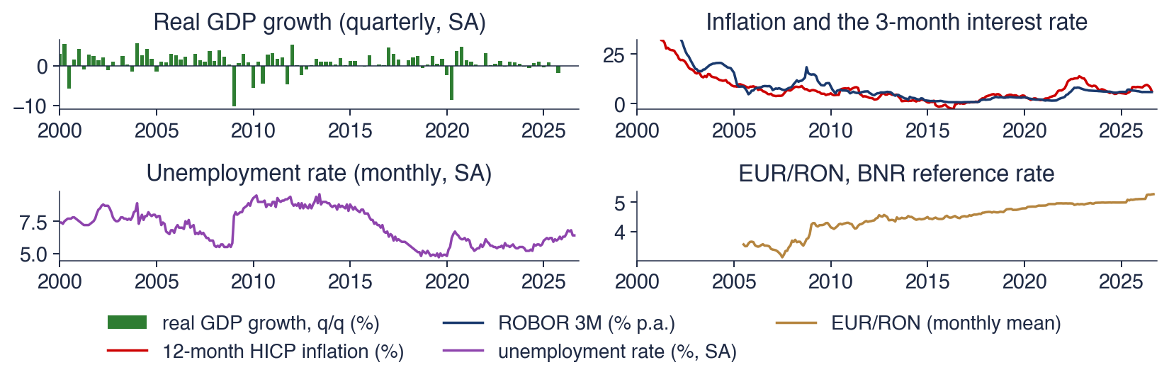
 TSA_ch6_multivariate_data