Bucharest University of Economic Studies IDA Institute Digital Assets Blockchain Research Center AI4EFin Artificial Intelligence for Energy Finance Romanian Academy, Institute for Economic Forecasting MSCA Digital Finance
What do option prices reveal about the future distribution?
“If options are correctly priced in the market, it should not be possible to make sure profits by creating portfolios of long and short positions in options and their underlying stocks.” — Black & Scholes (1973)
Black–Scholes: replication gives a single implied volatility per asset
daily delta hedging, three-month call: error standard deviation \(9.5\%\) of the premium
The smile: one-month implied volatility from the historical distribution of the S&P 500 (Standard & Poor's)
\(30.6\%\) at \(K/S = 0.8\), against \(13.9\%\) at the money
Bitcoin, 38-day expiry: risk-neutral probability of a fall of more than \(30\%\)
\(1.24\%\), against \(0.14\%\) under the log-normal benchmark
S&P 500, 1990–2026: mean VIX (CBOE Volatility Index) \(19.4\), mean realised volatility \(15.3\)
variance risk premium: \(4.09\) vol points, positive on \(86\%\) of days
If options are correctly priced in the market, it should not be possible to make sure profits by creating portfolios of long and short positions in options and their underlying stocks.
Black & Scholes (1973) obtain the price of an option from the absence of arbitrage: a portfolio of the stock and cash, rebalanced continuously, replicates the option, and its price does not depend on the stock's expected return. In this model all options on the same asset have the same implied volatility. Replication in practice is discrete. In the chapter's simulation, daily delta hedging of a three-month call leaves an error with a standard deviation of 9.5% of the premium, and weekly rebalancing one of 21.5%.
Market prices do not respect the assumption of a single volatility. Since the crash of October 1987, low-strike puts have been much more expensive than at-the-money options, and implied volatility depends on the strike: the smile and the skew. The historical distribution of 9,225 overlapping monthly S&P 500 (Standard & Poor's) returns gives a one-month implied volatility of 30.6% at a strike of 80% of the current price and of 13.9% at the money. Option prices therefore allow one to recover the risk-neutral distribution of the future price. On the Bitcoin option surface of 22 September 2026, at the 38-day expiry, the probability of a fall of more than 30% is 1.24%, against 0.14% under the log-normal benchmark. These probabilities are prices of insurance, not forecasts.
The gap between the volatility priced by the market and realised volatility is measurable. Over 9,203 days in 1990–2026, the VIX (CBOE Volatility IndeX) has a mean of 19.4, and the realised volatility of the S&P 500 over the next 21 trading days a mean of 15.3. The ex-post variance risk premium (VRP) is 4.09 vol points, with a Newey–West standard error of 0.27, and it is positive on 86% of days. The exceptions are crashes: the worst value, −72.0 points, belongs to the window starting on 20 February 2020. As a forecast of next month's variance, the VIX has a Mincer–Zarnowitz slope of 0.86, and the joint test rejects unbiasedness. The chapter therefore studies what information options carry about future risk and with which standard errors it must be read.
Implied versus realised volatility of the S&P 500, 1990–2026: top, the VIX and the realised volatility over the next 21 trading days; bottom, their difference, the ex-post variance risk premium, in vol points. Interactive chart: “Implied vs Realised Volatility, S&P 500 (1/2)” →
What you will be able to do
Derive put–call parity, the binomial price and the Black–Scholes equation.
Compute the Greeks, the discrete-hedging error and an arbitrage-free SVI (Stochastic Volatility Inspired, parameterisation) surface with its density and confidence bands.
Interpret option-implied forecasts (VIX, variance risk premium) with the right standard errors.
An option pays only in some states of the world, so its price depends on the distribution of the underlying asset at expiry, not only on the direction in which the price is expected to move. The chapter first derives option prices from the absence of arbitrage and then reads the prices observed in the market as information about future volatility and about crash risk. Throughout, \(S_t\) is the price of the underlying at time \(t\),\(K\) the strike, \(T\) the expiry, \(\tau = T - t\) the time left in years and \(r\) the continuously compounded risk-free rate; the full notation is in Further Topics.
A put with a low strike pays only after a large fall of the underlying, and a call with a high strike only after a large rise. The prices of such contracts therefore measure how the market values particular regions of the distribution of the future price. Taken across many strikes and expiries, option prices reveal what the market expects about volatility and about crashes, and at what price it insures against them.
The chapter has two parts:
Part I prices options by replication: put–call parity, static spanning of a pay-off with options, the binomial tree, the Black–Scholes equation, the sensitivities of the price (the Greeks) and the error left by hedging at discrete dates. It then introduces implied volatility, the smile and a full Bitcoin option surface with its risk-neutral density.
Part II reads implied volatility as information: variance swaps and the VIX, the Cboe index of 30-day S&P 500 implied volatility, the variance risk premium and 0DTE options, which have zero days to expiry.
Two case studies follow: lower bounds on the equity premium computed from option prices, and the reaction of the VIX to volatility shocks. The last part applies the discovery loop with an artificial intelligence (AI) assistant to an open question about the variance risk premium.
In brief
An option pays only in some states: its price is a bet on the distribution
not only on the direction
so it reveals what the market expects about volatility and crashes
Part I, pricing by replication
parity, static spanning, the binomial tree
the Black–Scholes equation, the Greeks and the discrete-hedging error
Then implied volatility, the smile and a full Bitcoin surface with its risk-neutral density
Part II, implied volatility as information
variance swaps and the VIX (the Cboe index of 30-day S&P 500 implied volatility)
the variance risk premium and 0DTE options (zero days to expiry)
Case studies: option-implied bounds on the equity premium and how the VIX reacts to volatility shocks
AI (artificial intelligence) for scientific discovery
What you should be able to do
derive put–call parity, the binomial price and the Black–Scholes equation
compute the Greeks, the discrete-hedging error and an arbitrage-free SVI (Stochastic Volatility Inspired, parameterisation) surface with its density and bands
interpret option-implied forecasts (VIX, variance risk premium) with the right standard errors
Further Topics and Appendix: reading for familiarity
The Chicago Board Options Exchange (Cboe) opened in 1973, as the first exchange for standardised, listed options (MacKenzie & Millo, 2003). Before it, options were negotiated one by one, over the counter, with terms set by the two parties. The photograph shows the trading floor of the Chicago Board of Trade in 2006; its members founded the Cboe.
The pricing papers of Black & Scholes (1973) and Merton (1973) appeared in the same year. MacKenzie & Millo (2003) document that traders soon used the formula on the floor: the theory changed the market it described. The prices later used to test the model were therefore set by traders who already used it.
The key idea of Black & Scholes (1973) is that a portfolio of the stock and cash, adjusted continuously, can replicate the pay-off of an option. If two positions have the same pay-off in every state, they must have the same price, otherwise there is an arbitrage. The price of the option follows from this argument, without any assumption about investors' preferences or about the expected return of the stock.
Myron Scholes and Robert C. Merton received the 1997 Nobel Memorial Prize in Economic Sciences; Fischer Black had died in 1995. The derivation is given in the Black–Scholes section; the data and notation are in Further Topics.
Option prices depend on the distribution of the future price, so they carry information about volatility and crash risk. The first half of the chapter derives prices from replication; the second half uses the observed prices as data.
Parity and Static Replication
This section collects the results that follow from the absence of arbitrage alone. They hold for any model of the underlying price: put–call parity, the static replication of a smooth pay-off with a bond, a forward and a strip of options, and three consequences used later in the chapter, the variance strip, the risk-neutral density and finite option strategies. The options are European, with strike \(K\) and expiry \(T\);\(C\) and \(P\) denote the prices of a call and a put.
Put–Call Parity: What Does No Arbitrage Alone Imply?
Consider two portfolios, built today from European options with the same strike \(K\) and expiry \(T\) on a stock without dividends. Portfolio A holds one call and cash \(K e^{-r\tau}\), which grows to \(K\) at \(T\); its pay-off is \(\max(S_T, K)\). Portfolio B holds one put and one share; its pay-off is \(\max(K, S_T)\). The two portfolios pay the same amount in every state of the world, so they must cost the same today:
\[C_t - P_t = S_t - K e^{-r\tau}.\]
(12.1)
If the left-hand side of (12.1) exceeded the right-hand side, an investor could sell portfolio A, buy portfolio B and keep the difference today, with a zero net pay-off at \(T\); the opposite inequality is exploited the other way round. With a continuous dividend yield \(q\),\(S_t\) is replaced by \(S_t e^{-q\tau}\).
The argument uses no model for \(S\): parity follows from the absence of arbitrage alone (Merton, 1973). A consequence is used throughout the chapter. The Black–Scholes prices of a call and a put satisfy (12.1) for every value of \(\sigma\), so a volatility that reproduces the market price of the call also reproduces the market price of the put. A call and a put with the same \(K\) and \(T\) therefore have the same implied volatility.
In brief
Two portfolios with the same pay-off at \(T\) (European options, same \(K\) and \(T\), no dividends):
A: one call + cash \(K e^{-r\tau}\) (worth \(K\) at \(T\)) \(\Rightarrow\)\(\max(S_T, K)\)
B: one put + one share \(\Rightarrow\)\(\max(K, S_T)\)
Same pay-off in every state, so the same price today, otherwise there is an arbitrage:
\(C_t - P_t = S_t - K e^{-r\tau}\) (with dividend yield \(\delta\): \(S_t e^{-\delta\tau}\) instead of \(S_t\))
No model for \(S\) is needed: parity uses only no-arbitrage Merton (1973)
Consequence: a call and a put with the same \(K\) and \(T\) have the same implied volatility
Static Replication: Any Pay-Off from a Bond, a Forward and Options
Parity replicates one pay-off with a put, a call, a share and cash. The spanning result of Carr and Madan generalises it to any twice-differentiable pay-off \(f(S_T)\). For any point \(F\), Taylor's formula with integral remainder gives
where \((x)^+ = \max(x, 0)\). The proof, by integration by parts, is in the Appendix.
The terms of (12.2) are positions in traded contracts. The constant \(f(F)\) is a zero-coupon bond, \(f'(F)(S_T - F)\) is \(f'(F)\) forward contracts with delivery price \(F\), and the two integrals are strips of puts with strikes below \(F\) and calls with strikes above \(F\), with \(f''(K)\,dK\) options at each strike. The curvature of the pay-off is bought with options; its level and slope with a bond and a forward.
Each piece has a market price today: the bond costs \(e^{-r\tau}\) per unit, a forward with delivery price equal to the forward price \(F\) costs 0, and the options cost \(P(K)\) and \(C(K)\), today's put and call prices at strike \(K\). The value of the pay-off today is therefore
whatever the model for \(S\)(Bakshi, Kapadia & Madan, 2003). No pricing measure is needed for \(V_0\). The pricing measure \(Q\) of Section 3 is needed only to read option prices as expectations, as in the density result of the next slide.
In brief
Carr–Madan spanning: any twice-differentiable pay-off \(f(S_T)\) and any point \(F\):
Taylor with integral remainder; proof in the Appendix
\(P(K)\), \(C(K)\): today's put and call prices at strike \(K\), whatever the model for \(S\)Bakshi, Kapadia & Madan (2003)
Why this price: each piece has a market price today
the bond \(e^{-r\tau}\) per unit, the forward 0, the options \(P(K)\) and \(C(K)\)
No model for \(S\) and no pricing measure are needed for \(V_0\); the measure \(Q\) of Section 3 is needed only to read option prices as expectations, as in the density bullet of the next slide
A price is called "risk-neutral" when it is the discounted mean pay-off under the pricing measure \(Q\), not under the real-world probabilities. The measure \(Q\) is constructed in Section 3, on the binomial tree. Three applications of (12.2) recur in the chapter.
The first is variance. The pay-off \(f(S) = -2\ln(S/F)\) has \(f''(K) = 2/K^2\), so it is replicated by a strip of out-of-the-money (OTM) options with weights proportional to \(1/K^2\). This strip is the variance swap and the VIX of Section 8. Low strikes receive the largest weights, so an expensive put wing makes variance expensive.
The second is the density. A butterfly spread, long one call at \(K - h\) and one at \(K + h\) and short two calls at \(K\), where \(h\) is the strike step, costs \(C(K - h) - 2C(K) + C(K + h)\); divided by \(h^2\), this price converges to the second derivative of the call price in the strike. Breeden & Litzenberger (1978) show that this derivative is the discounted risk-neutral density \(q\) of \(S_T\):
The risk-neutral density is thus a price, recovered from a continuum of call prices (Section 7).
The third concerns common strategies. Straddles, spreads and protective puts are finite strips, with \(f''\) concentrated at one or two strikes. Pay-offs that are powers of the log return give the risk-neutral moments, and the pay-off \(S^2\) gives SVIX, the simple VIX of Martin (2017); both are in the Appendix.
In brief
“Risk-neutral”: a price is the discounted mean pay-off under the pricing measure \(Q\)
not under real-world probabilities
\(Q\) is constructed in Section 3
Variance: \(f(S) = -2\ln(S/F)\) has \(f''(K) = 2/K^2\)
the strip with weights \(1/K^2\) is the variance swap and the VIX (Section 8)
Low strikes get the largest weights, so an expensive put wing makes variance expensive
Parity (12.1), the spanning formula (12.2) and the density (12.3) need no model for the underlying. They turn option prices into the prices of other pay-offs: the forward, variance and the probability of each region of \(S_T\).
The Binomial Tree
The binomial tree is the simplest model in which an option can be replicated dynamically. It shows how the pricing measure \(Q\) arises from replication, why the real probability of an up move does not enter the price, and how, with many steps, the tree converges to the Black–Scholes model.
The Binomial Tree: How Do We Price an Option by Replication?
Over one period of length \(\Delta t\), the stock moves from \(S\) to \(uS\) or to \(dS\), where \(u\) and \(d\) are the up and down factors. The gross riskless return is \(R = e^{r\Delta t}\), and absence of arbitrage requires \(d < R < u\). A call worth \(C_u\) after an up move and \(C_d\) after a down move is replicated by \(\Delta\) shares and cash \(B\) if \(\Delta uS + RB = C_u\) and \(\Delta dS + RB = C_d\).
The two equations give \(\Delta = (C_u - C_d)/[(u - d)S]\), and the price of the call is the cost of the replicating portfolio:
\[C = \Delta S + B = \frac{q\,C_u + (1 - q)\,C_d}{R}, \qquad q = \frac{R - d}{u - d}.\]
(12.4)
Because \(d < R < u\),\(q\) lies in \((0, 1)\). It is the unique probability under which the discounted stock price \(S_t/R^t\) is a martingale; on the tree, \(q\) denotes this probability, not the dividend yield. The real probability of an up move never enters (12.4): risk preferences are already contained in the stock price \(S\).
The fundamental theorem of asset pricing generalises this result: as shown by Harrison & Pliska (1981) and, in full generality, by Delbaen & Schachermayer (1994), there is no arbitrage if and only if there exists an equivalent martingale measure \(Q\).\(Q\) is unique exactly when the market is complete. With jumps or stochastic volatility there are many measures \(Q\), and option prices carry risk premia, the subject of Section 8.
In brief
One period of length \(\Delta t\): \(S \to uS\) or \(dS\), with \(d < R = e^{r\Delta t} < u\)
\(u\), \(d\): up and down factors
\(R\): gross riskless return
Replicate the call with \(\Delta\) shares and cash \(B\): \(\Delta uS + RB = C_u\) and \(\Delta dS + RB = C_d\)
\(C_u\), \(C_d\): the call values after an up and a down move
Solution: \(\Delta = \dfrac{C_u - C_d}{(u - d)S}\), and the price is \(C = \Delta S + B = \dfrac{q\,C_u + (1 - q)\,C_d}{R}\)
\(q = \dfrac{R - d}{u - d} \in (0, 1)\) (the risk-neutral probability, the discrete analogue of the density \(q(K)\)) is the unique probability under which \(S_t/R^t\) is a martingale
\(Q\) is unique exactly when the market is complete; with jumps or stochastic volatility there are many \(Q\), and option prices carry risk premia (Section 8)
The CRR Tree: \(N\) Steps and Convergence to Black–Scholes
One period has only two final states. With \(N\) steps the tree has \(N + 1\) final states, which approximate the distribution of \(S_T\). The Cox–Ross–Rubinstein (CRR) tree (Cox, Ross & Rubinstein, 1979) sets \(\Delta t = T/N\),\(u = e^{\sigma\sqrt{\Delta t}}\) and \(d = 1/u\). This choice gives the one-step log return the variance \(\sigma^2\Delta t\) up to terms of order \(\Delta t^2\), so as \(N\) grows the tree converges to the geometric Brownian motion of the Black–Scholes model. The risk-neutral probability \(q = (e^{r\Delta t} - d)/(u - d)\) is the same at every node.
A European call depends only on the final node, reached after \(j\) up moves and \(N - j\) down moves. Applying (12.4) backwards through the \(N\) steps gives
the discounted risk-neutral mean of the pay-off, with a binomial distribution for the number of up moves \(j\).
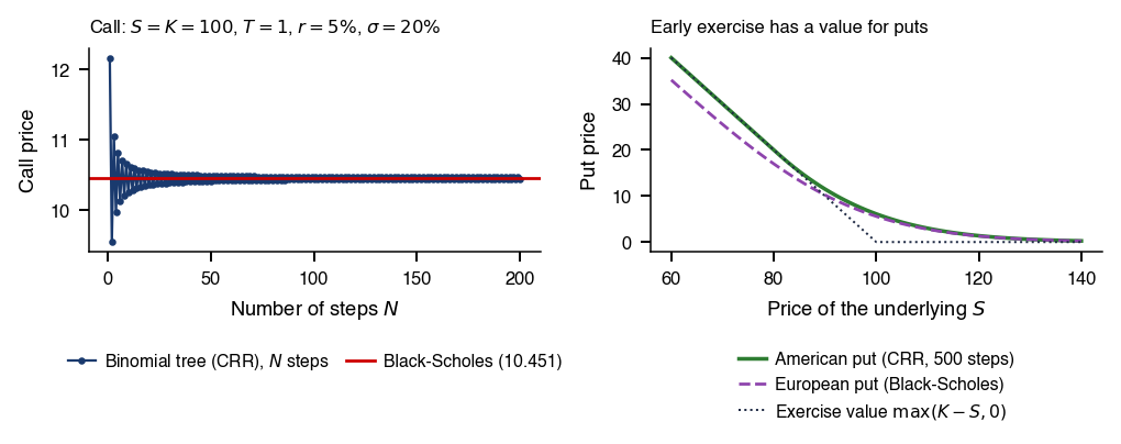
An American option can be exercised at any time up to \(T\), so it is valued backwards from \(T\), taking at every node the larger of the continuation value and the exercise value. The convergence of (12.5) to the Black–Scholes price and the early-exercise premium of an American put are shown in Further Topics.
In brief
Why \(N\) steps: one period has only two final states
with \(N\) steps the \(N + 1\) final states approximate the distribution of \(S_T\)
The CRR (Cox–Ross–Rubinstein) tree Cox, Ross & Rubinstein (1979): \(\Delta t = T/N\), \(u = e^{\sigma\sqrt{\Delta t}}\), \(d = 1/u\)
This choice gives the one-step log return the variance \(\sigma^2\Delta t\) (up to terms of order \(\Delta t^2\)), so the tree converges to the geometric Brownian motion of the Black–Scholes model
\(q = (e^{r\Delta t} - d)/(u - d)\) is the same at every node
On the tree, replication defines the price and the probability \(q\) under which discounted prices are martingales; the real-world probability of an up move plays no role. With \(N\) steps the CRR tree approximates the geometric Brownian motion, the model of the next section.
Black–Scholes and the Greeks
In continuous time, replication leads to a partial differential equation. This section derives the Black–Scholes equation, gives its solution for European options and defines the Greeks, the partial derivatives of the price. The Greeks measure the exposures of an option position and are the quantities a hedger adjusts.
The Black–Scholes Equation: What Price Does Continuous Replication Give?
The model assumes that the stock follows a geometric Brownian motion (GBM), \(dS_t = \mu S_t\,dt + \sigma S_t\,dW_t\), with constant volatility \(\sigma\) and constant rate \(r\); trading is continuous, without costs, and short selling is allowed. The option value \(V(S, t)\) is to be replicated by a self-financing portfolio \(\Pi\) of \(\Delta_t\) shares and cash \(B_t\) invested at \(r\), whose value changes only through gains: \(d\Pi = \Delta\,dS + rB\,dt\).
By Itô's lemma, the option value evolves as
\[dV = \big(V_t + \mu S V_S + \tfrac{1}{2}\sigma^2 S^2 V_{SS}\big)\,dt + \sigma S V_S\,dW_t,\]
where \(V_t\),\(V_S\) and \(V_{SS}\) are partial derivatives. Choosing \(\Delta = V_S\) and starting from \(\Pi = V\), so that \(B = V - S V_S\), gives \(d(V - \Pi) = \big(V_t + \tfrac{1}{2}\sigma^2 S^2 V_{SS} - rB\big)\,dt\). Both the Brownian increment \(dW_t\) and the drift \(\mu\) drop out.
The difference \(V - \Pi\) starts at zero and is riskless. A riskless position that costs nothing must earn nothing, which gives the Black–Scholes equation of Black & Scholes (1973) and Merton (1973):
\[V_t + \tfrac{1}{2}\sigma^2 S^2 V_{SS} + r S V_S - r V = 0, \qquad V(S, T) = \text{pay-off}.\]
(12.6)
That \(\mu\) is irrelevant is a result of replication, not an assumption. By the Feynman–Kac formula, the solution of (12.6) is \(V = e^{-r\tau}E^Q[\text{pay-off}]\), where under \(Q\) the stock drifts at the rate \(r\).
where \(\Phi\) is the distribution function of the standard Normal distribution. With a dividend yield \(q\),\(S\) is replaced by \(S e^{-q\tau}\).
The two terms have a direct reading. \(\Phi(d_2)\) is the risk-neutral probability that the call ends in the money, so the second term is the present value of paying \(K\) in those states. \(\Phi(d_1)\) is the number of shares in the replicating portfolio, the delta. The put formula follows from the call formula and parity (12.1).
The formula has five inputs. The price \(S\), the strike \(K\), the time to expiry \(\tau\) and the rate \(r\) are observed. Volatility \(\sigma\) is the only input that is not observed: it must be estimated from past prices or implied from option prices, the subject of Section 6.
In brief
European call and put, no dividends (with yield \(\delta\): replace \(S\) by \(S e^{-\delta\tau}\)):
\(C = S\,\Phi(d_1) - K e^{-r\tau}\,\Phi(d_2), \qquad P = K e^{-r\tau}\,\Phi(-d_2) - S\,\Phi(-d_1)\)
\(d_1 = \dfrac{\ln(S/K) + (r + \sigma^2/2)\tau}{\sigma\sqrt{\tau}}, \qquad d_2 = d_1 - \sigma\sqrt{\tau}\), with \(\Phi\) the standard Normal distribution function
Reading the two terms:
\(\Phi(d_2)\) = risk-neutral probability that the call ends in the money
\(\Phi(d_1)\) = number of shares in the replicating portfolio (the delta)
Five inputs: \(S\), \(K\), \(\tau\), \(r\) observed
\(\sigma\) is the only one not observed: it must be estimated or implied
The Greeks are the partial derivatives of the option price with respect to its inputs. Delta \(\Delta = \partial C/\partial S\) is the hedge ratio, gamma \(\Gamma = \partial^2 C/\partial S^2\) the rate at which delta changes with the price, vega \(\mathcal{V} = \partial C/\partial\sigma\) the sensitivity to volatility, theta \(\Theta = \partial C/\partial t\) the change of value with the passage of time and rho \(= \partial C/\partial r\) the sensitivity to the rate. The formulas are on the next slide.
The interactive chart has four panels, for the delta, gamma, vega and theta of a call with strike \(K = 100\). In each panel the horizontal axis is the price of the underlying \(S\), from 60 to 140, and the curves correspond to three expiries: one month, three months and one year. The first slider sets the volatility \(\sigma\) and the second marks a price \(S\) on the curves. The ▶ button raises \(\sigma\) step by step.
Question for the room Press ▶: volatility σ rises from 10% to 50%. What happens to the gamma of the three-month call at S = K = 100?
Answer
It falls from 0.078 to 0.016, almost like 1/σ, while vega stays almost constant (0.194 at σ = 10%, 0.197 at σ = 50%). At K = 100 and σ = 20%, the one-month call has the largest gamma (0.069, against 0.039 at three months and 0.019 at one year) and the fastest time decay (theta −0.043 a day), and the one-year call has the largest vega (0.381 per volatility point). Vega per unit change in σ is ΓS²στ. Per percentage point of volatility, vega is ΓS²στ/100: for the three-month call at S = K = 100 and σ = 20%, it equals 0.197.
Short maturities concentrate gamma and theta at the strike, and long maturities carry the most vega. On the chart, vega is measured per volatility point and theta per calendar day.
For the Black–Scholes call (12.7), delta is \(\Delta = \Phi(d_1)\), and the put delta is \(\Phi(d_1) - 1\). Gamma is \(\Gamma = \varphi(d_1)/(S\sigma\sqrt{\tau})\), where \(\varphi\) is the standard Normal density. The derivation of all the Greeks rests on one identity, \(S\varphi(d_1) = K e^{-r\tau}\varphi(d_2)\), which makes the terms coming from the derivatives of \(d_1\) and \(d_2\) cancel.
so for one expiry gamma and vega are proportional. Theta follows from the Black–Scholes equation (12.6):\(\Theta = rC - rS\Delta - \tfrac{1}{2}\sigma^2 S^2 \Gamma\). Rho is \(K\tau e^{-r\tau}\Phi(d_2)\). The derivations are exercises A1 and A7 of Seminar 12.
The expression for theta shows the trade-off of a hedged option. For a delta-hedged position, the gain from gamma when the stock moves and the loss from theta as time passes cancel on average in the model. The proportionality (12.8) links gamma risk to volatility risk and is used in Section 5 to size the profit and loss (P&L) of a hedged option.
The Black–Scholes price follows from continuous replication and does not depend on the drift \(\mu\). Its only unobserved input is volatility. The Greeks measure the exposures of an option, and (12.8) ties gamma to vega.
Delta Hedging in Practice
Black–Scholes replication requires continuous rebalancing, which no trader can carry out. This section measures the error left when the hedge is adjusted at \(N\) dates, shows how it falls with \(N\), and derives the P&L of a hedged option when realised volatility differs from the volatility at which the option was sold.
Discrete Delta Hedging: How Much Risk Is Left with \(N\) Rebalancings?
In practice the hedge is adjusted \(N\) times, at the dates \(t_i = iT/N\). At \(t_0 = 0\) the hedger sells the call at its Black–Scholes price \(C_0\), buys \(\Delta_0 = \Phi(d_1)\) shares and keeps the cash \(B_0 = C_0 - \Delta_0 S_0\). At each date \(t_i\),\(i = 1, \dots, N - 1\), the position is rebalanced to the new delta, \(\Delta_i = \Phi\big(d_1(S_{t_i}, T - t_i)\big)\), and the purchase or sale of shares is financed from the cash account, which earns interest:
The portfolio is therefore self-financing. At expiry the hedger holds \(\Delta_{N-1}\) shares and the cash, and pays the call pay-off. The hedging error is
With continuous rebalancing in the Black–Scholes model, \(\varepsilon_N\) would be zero on every path.
The chapter's simulation uses a geometric Brownian motion with drift \(\mu = 8\%\) and volatility \(\sigma = 20\%\), a call with \(S_0 = K = 100\), a rate \(r = 4\%\) and an expiry \(T = 0.25\) years, and 20,000 paths for each of \(N = 3\), 12, 63 and 252 rebalancings. The drift is deliberately different from \(r\): replication never uses \(\mu\), and a real drift different from \(r\) shows that the error stays centred at 0.
The interactive chart has two panels. On the left, the horizontal axis is the hedging error at expiry (12.9), per option, and the vertical axis its density across the 20,000 paths. On the right, the horizontal axis is the number of rebalancings \(N\) and the vertical axis the standard deviation of the error in % of the premium, both on logarithmic scales; the reference line has slope \(-1/2\), the rate \(1/\sqrt{N}\). The slider chooses the rebalancing frequency, and the ▶ button steps through the frequencies.
Question for the room With daily rebalancing, the standard deviation of the error is 9.5% of the premium. How much more often must the hedge be adjusted to halve it?
Answer
About four times as often. Doubling N approximately halves the error variance, not its standard deviation: the standard deviation falls like 1/√N (the estimated log-log slope is −0.48). Halving the standard deviation requires approximately four times as many rebalancings: from 63 to 252 over the three months. In the simulation, the standard deviation falls from 9.5% to 4.8% of the premium. Transaction costs, however, grow with N: like N with a fixed cost per rebalancing, roughly like √N with costs proportional to the traded value.
The Black–Scholes premium is 4.49, with \(d_1 = 0.15\). The mean error is close to 0 for every frequency. The standard deviation, in % of the premium, is 40.8% with monthly rebalancing, 21.5% weekly, 9.5% daily and 4.8% four times a day. The estimated slope on the log axes is \(-0.48\).
The error of discrete hedging comes from gamma. Between two rebalancing dates the delta held is fixed, while the delta required by the model moves with the price; the position gains or loses according to whether the squared return over the interval is below or above its expected value \(\sigma^2\Delta t\). These local errors have mean close to zero and are approximately uncorrelated, so their variance adds up over the \(N\) intervals and the standard deviation of the total falls like \(1/\sqrt{N}\). The Appendix derives the approximation
The approximation matches the simulation. For \(N = 12\), 63 and 252, (12.10) gives 1.01, 0.44 and 0.22, against simulated standard deviations of 0.96, 0.43 and 0.22, in currency units per option. In the left tail, the worst 1% of paths lose 2.68 per option with weekly rebalancing and 1.17 with daily rebalancing. Halving the standard deviation of the error requires about four times as many rebalancings.
Rebalancing more often is not free. With a fixed cost per rebalancing, the total cost grows like \(N\). With costs proportional to the traded value, in the standard diffusion setting, the expected cost grows roughly like \(\sqrt{N}\). The hedging frequency is therefore chosen by trading off the error (12.10) against the cost model.
In brief
Left: distribution of the error \(\varepsilon_N\) for four rebalancing frequencies
right: standard deviation of the error, in % of the premium, against \(N\) on log axes
Black–Scholes premium \(4.49\) and \(d_1 = 0.15\)
Mean error near 0
standard deviation (s.d.) in % of the premium: monthly \(40.8\%\), weekly \(21.5\%\), daily \(9.5\%\), four times a day \(4.8\%\)
worst 1% of paths, in currency units per option: \(-2.68\) (weekly), \(-1.17\) (daily)
Log-log slope \(-0.48\)
theory (Appendix): s.d. \(\approx \sqrt{\pi/4}\,\mathcal{V}\sigma/\sqrt{N}\) (\(\mathcal{V}\): vega)
theory \(1.01\), \(0.44\), \(0.22\) vs simulated \(0.96\), \(0.43\), \(0.22\) (\(N = 12, 63, 252\))
Transaction costs depend on the cost model
with a fixed cost per rebalancing, the total cost grows like \(N\)
with costs proportional to the traded value, in the standard diffusion setting, the expected cost grows roughly like \(\sqrt{N}\)
Suppose the option is sold at the implied volatility \(\sigma_{imp}\) and hedged with \(\Delta = \partial_S V^{imp}\), where \(V^{imp}\) is its Black–Scholes value at \(\sigma_{imp}\), while the price moves with the realised volatility \(\sigma_{real}\):\(dS = \mu S\,dt + \sigma_{real} S\,dW_t\). By Itô's lemma, \(dV = V_t\,dt + \Delta\,dS + \tfrac{1}{2}\Gamma\sigma_{real}^2 S^2\,dt\), and the Black–Scholes equation at \(\sigma_{imp}\) gives \(V_t = rV - rS\Delta - \tfrac{1}{2}\sigma_{imp}^2 S^2\Gamma\).
The position short one option, long \(\Delta\) shares and with cash at \(r\) is self-financing, and its P&L evolves as \(d\,\text{P\&L} = r\,\text{P\&L}\,dt + \tfrac{1}{2}\Gamma_t S_t^2(\sigma_{imp}^2 - \sigma_{real}^2)\,dt\). Over the life of the option,
The P&L (12.11) depends on the path: the variance gap is weighted by \(\Gamma_t S_t^2\), which is large when the price is near the strike and when expiry is near.
A short variance swap pays \(\sigma_{imp}^2 - \sigma_{real}^2\) with constant weights. A delta-hedged option is therefore a bet on variance with random weights. Its first-order size follows from (12.8): with \(\mathcal{V} = \Gamma S^2\sigma\tau\),
the equation at \(\sigma_{imp}\) gives \(V_t = rV - rS\Delta - \tfrac{1}{2}\sigma_{imp}^2 S^2 \Gamma\)
Short option + \(\Delta\) shares + cash at \(r\), self-financing; its profit and loss (P&L):
\(d\,\text{P\&L} = r\,\text{P\&L}\,dt + \tfrac{1}{2}\,\Gamma_t S_t^2\left(\sigma_{imp}^2 - \sigma_{real}^2\right)dt\), so over the life
\(\text{P\&L} = \displaystyle\int_0^T e^{r(T - t)}\,\tfrac{1}{2}\,\Gamma_t S_t^2\left(\sigma_{imp}^2 - \sigma_{real, t}^2\right)dt\): path-dependent, weighted by \(\Gamma\), large near \(K\) and near \(T\)
A short variance swap pays \(\sigma_{imp}^2 - \sigma_{real}^2\) with constant weights
a delta-hedged option is a variance bet with random weights
First-order size: vega \(\times\) (implied \(-\) realised), checked on the next slide
The simulation sells a three-month call at an implied volatility of 20% and hedges it daily, while the realised volatility is 15%, 20% or 25%. By (12.11), the seller gains when realised volatility is below implied volatility and loses when it is above; when the two are equal, only the discrete-hedging noise of the previous slides remains.
The interactive chart shows the density of the seller's P&L across the simulated paths, with the P&L of the hedged three-month call on the horizontal axis. The slider sets the realised volatility, and the ▶ button moves it step by step.
Question for the room A three-month call is sold at 20% implied volatility and hedged daily. On what share of the paths does the seller gain if realised volatility is 25%?
Answer
In this simulation, the seller gains on 2.2% of the paths. Mean P&L is −0.99 per option and its standard deviation is 0.68. The first-order approximation is vega × (implied volatility − realised volatility), or 0.197 × (20 − 25) ≈ −0.99. Daily rebalancing leaves a discrete hedging error, so some paths still produce positive P&L. With realised volatility of 15%, the mean is +0.98, positive on 99.8% of the paths.
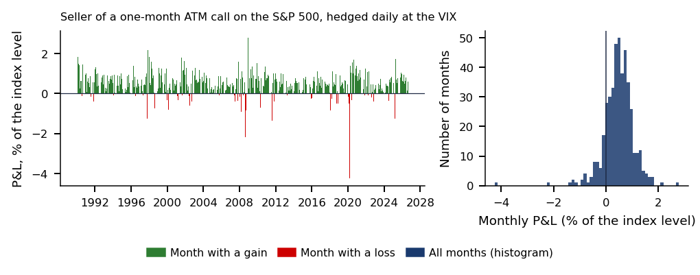
With realised volatility of 15%, the mean P&L is \(+0.98\) and the P&L is positive on 99.8% of the paths. At 20%, the mean is \(+0.00\) and only the discrete-hedging noise remains, with a standard deviation of 0.43. At 25%, the mean is \(-0.99\) and the P&L is positive on only 2.2% of the paths. Each mean is close to vega times 5 volatility points, \(0.197 \times 5 \approx \pm 0.99\). A delta-hedged option is a clean bet on volatility. The same strategy on 36 years of S&P 500 data is in Further Topics.
In brief
Three-month call sold at 20% implied volatility, hedged daily
realised volatility 15%, 20% or 25%
Realised 15%: mean P&L \(+0.98\), positive on \(99.8\%\) of paths
Realised 20%: mean \(+0.00\); only discrete-hedging noise remains (s.d. \(0.43\))
Realised 25%: mean \(-0.99\), positive on only \(2.2\%\) of paths
Each mean is close to vega \(\times\) 5 vol points \(= 0.197 \times 5 \approx \pm 0.99\)
Discrete hedging leaves an error whose standard deviation falls like \(1/\sqrt{N}\): 21.5% of the premium weekly and 9.5% daily in the simulation. When realised volatility differs from implied volatility, the hedged option earns or loses approximately vega times the volatility gap, with the gamma weights of (12.11).
Implied Volatility and the Smile
If the Black–Scholes model were right, a single volatility would price all options on an asset. Market prices contradict this. This section defines implied volatility, describes the smile that appeared after the crash of October 1987, lists its economic sources and compares three ways of producing it: the historical distribution of returns, a jump model and a stochastic-volatility model.
Implied Volatility: Which \(\sigma\) Explains the Market Price?
Implied volatility\(\sigma_{imp}\) is the value of \(\sigma\) that makes the Black–Scholes price equal to the observed market price:
\[BS(S, K, \tau, r, \sigma_{imp}) = C^{market},\]
(12.12)
where \(BS(\cdot)\) is the formula (12.7) and \(C^{market}\) the observed price. The solution is unique because vega is positive: the price increases strictly in \(\sigma\). There is no closed form, because \(\sigma\) enters both \(\Phi(d_1)\) and \(\Phi(d_2)\), so (12.12) is solved numerically; the Newton method is in Further Topics.
Traders quote options in implied volatility, not in money. Implied volatility removes the effect of the strike, the maturity and the price level, so it is comparable across strikes, maturities and assets.
Implied volatility is also a test of the model. If Black–Scholes were right, all options on one asset would have the same implied volatility, whatever their strike and expiry. The rest of the section shows that they do not.
In brief
Implied volatility\(\sigma_{imp}\): the \(\sigma\) that makes the Black–Scholes price equal the market price
\(BS(S, K, \tau, r, \sigma_{imp}) = C^{market}\); \(BS(\cdot)\): the Black–Scholes formula, \(C^{market}\): the observed price
The solution is unique because vega \(> 0\): the price increases in \(\sigma\)
There is no closed form: \(\sigma\) enters both \(\Phi(d_1)\) and \(\Phi(d_2)\), so the equation is solved numerically
Traders quote options in implied volatility, not in money
it is comparable across strikes, maturities and assets
If Black–Scholes were right, all options on one asset would have the same implied volatility
Before 1987, index options had a nearly flat implied volatility across strikes (Rubinstein, 1994). Since the crash of October 1987, low-strike puts are much more expensive than at-the-money options: implied volatility falls with the strike, a pattern called the skew. The photograph shows the Amsterdam stock exchange after the crash, on 21 October 1987.
Bates (1991) finds that option prices showed fears of a crash between October 1986 and August 1987, but not strongly in the two months immediately before the crash. Crash risk was priced, but its timing was not.
The terminology is used throughout the chapter. The smile is implied volatility as a function of the strike \(K\), the term structure is implied volatility as a function of the expiry \(T\), and the surface is implied volatility as a function of both. Crash risk on the Bucharest Stock Exchange is studied by Pele & Mazurencu-Marinescu (2012).
Fat tails: large moves are more frequent than the Normal distribution allows (Chapter 1), so deep out-of-the-money options are worth more than Black–Scholes says.
Leverage and volatility feedback: when prices fall, volatility rises (Christie, 1982). The resulting negative skewness of returns makes low-strike puts dearer.
Crash fear: the market prices the risk of a negative jump, which is visible in put prices (Bates, 1991).
Demand for insurance: investors buy puts, and intermediaries, who cannot fully hedge the risk of the positions they take on, charge a premium for them (Gârleanu, Pedersen & Poteshman, 2009).
The first three mechanisms concern the distribution of returns; the fourth concerns who bears the risk.
In brief
Fat tails: large moves are more frequent than the Normal distribution allows (Chapter 1)
so deep OTM (Out-of-The-Money) options are worth more than Black–Scholes says
Leverage and volatility feedback: when prices fall, volatility rises Christie (1982)
negative skewness makes low-strike puts dearer
Crash fear: the market prices a negative jump risk, visible in put prices Bates (1991)
Each family of models produces a smile through a different mechanism. Jump models (Merton, 1976) add Poisson jumps to the Brownian motion; they fit steep short-dated smiles. In stochastic-volatility models (Heston, 1993; Hull & White, 1987) the variance follows its own mean-reverting process, correlated with the price; they fit the skew and the term structure of longer maturities.
Local-volatility models (Gatheral, 2006) read a volatility function \(\sigma(S, t)\) off the whole surface, with the formula of Dupire (1994); they match every quoted price today and are used to price exotic options. A parametric smile such as SVI (stochastic volatility inspired) (Gatheral & Jacquier, 2014) has five parameters per expiry and no dynamics; it serves for interpolation and quoting, and is used for the Bitcoin surface of Section 7.
The chart computes one-month implied volatilities from three sources: the historical distribution of S&P 500 returns, a Merton jump model and a Heston stochastic-volatility model, with the Black–Scholes constant volatility as a reference. The horizontal axis is moneyness \(K/S\) and the vertical axis implied volatility in %. The first slider sets the Heston price–variance correlation \(\rho\) and the second the mean jump of the Merton model, in log terms; the ▶ button moves \(\rho\) from \(-0.9\) to \(+0.9\).
The historical smile is obtained by pricing options with the empirical distribution of one-month returns, rescaled to a martingale with \(r = 0\) and no risk adjustment, and inverting (12.12) at each strike. It shows how much of the smile the shape of the realised distribution explains on its own.
Question for the room Press ▶: the Heston correlation ρ moves from −0.9 to +0.9. What happens to the Heston smile?
Answer
The tilt reverses: at ρ = +0.9, the Heston implied volatility is 10.7% at K/S = 0.8 and 28.2% at K/S = 1.2; at ρ = 0 the smile is nearly symmetric (23.7% and 22.4%). On the slide (ρ = −0.7), the highest implied volatility at K/S = 0.8 comes from the Merton jumps: 31.0%, against 16.3% ATM, close to the historical distribution (30.6%, against 13.9% ATM). Measured from the ATM level, the historical wing rises the most: 16.7 points, against 14.7 for Merton and 12.0 for Heston. Heston with ρ = −0.7 gives 28.6%, and its right wing is the lowest (14.6% at K/S = 1.2), because a negative correlation tilts the smile to the left.
On the slide, with \(\rho = -0.7\), the historical distribution gives 30.6% at \(K/S = 0.8\), against 13.9% at the money (ATM). The Merton jumps give 31.0% at \(K/S = 0.8\) against 16.3% ATM, and Heston 28.6% at \(K/S = 0.8\). The numbers are discussed on the next slide.
The historical smile uses 9,225 overlapping monthly S&P 500 returns, with skewness \(-1.27\) and excess kurtosis 6.8. The excess kurtosis requires a finite fourth moment, which Chapter 1 questions. Rescaled to a martingale, with \(r = 0\) and no risk adjustment, this distribution gives one-month implied volatilities of 30.6% at \(K/S = 0.8\), 13.9% at the money and 19.3% at \(K/S = 1.2\): a skew with a smaller rise on the right.
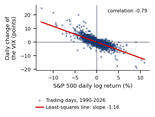
The Merton model, with one crash of about \(-8\%\) a year, gives 31.0% at \(K/S = 0.8\) against 16.3% at the money. The Heston model with a price–variance correlation \(\rho = -0.7\) gives 28.6% at \(K/S = 0.8\), 16.6% at the money and 14.6% at \(K/S = 1.2\); the negative correlation tilts its smile to the left. The leverage effect behind a negative \(\rho\) is measured on the S&P 500 and the VIX in Further Topics.
The historical smile has no risk adjustment, so it reflects only the shape of the realised distribution. Risk-neutral distributions are more left-skewed than realised ones (Jackwerth, 2000): the price of crash risk steepens market smiles further.
In brief
One-month implied volatility from three sources
the historical S&P 500 distribution, a jump model and a stochastic-volatility model
History: 9 225 overlapping monthly returns
skewness \(-1.27\), excess kurtosis \(6.8\)
the excess kurtosis requires a finite fourth moment, which Chapter 1 questions
rescaled to a martingale (\(r = 0\), no risk adjustment)
\(30.6\%\) at \(K/S = 0.8\), \(13.9\%\) ATM (At-The-Money), \(19.3\%\) at \(K/S = 1.2\)
Merton jumps (one crash of about \(-8\%\) a year): \(31.0\%\) at \(K/S = 0.8\) vs \(16.3\%\) ATM
Implied volatility is the volatility that reproduces a market price in the Black–Scholes formula. After 1987 it depends on the strike, because returns have fat tails and negative skewness and because crash risk is priced. Jumps, stochastic volatility and the historical distribution all produce a skew; the price of crash risk makes market smiles steeper.
Bitcoin Options and the Volatility Surface
This section describes a full option surface: all Bitcoin options listed on Deribit on 22 September 2026. Each expiry is fitted with the SVI parameterisation, the fits are checked against the no-arbitrage constraints, and the risk-neutral density of the 38-day expiry is recovered with bootstrap bands.
The Bitcoin Surface: How to Describe the Smile Without Arbitrage?
Deribit lists European options on Bitcoin, traded 24 hours a day, seven days a week. The options are inverse: the premium and the pay-off are paid in bitcoin (BTC), not in US (United States) dollars (USD). Each expiry has its own forward price \(F\), quoted by the exchange. DVOL (Deribit Volatility Index) is Deribit's 30-day implied-volatility index. The Further Topics show why the USD formulas still apply to inverse options.
The snapshot used in the chapter was taken on 22 September 2026 at 07:51 UTC (Coordinated Universal Time). It contains 9 expiries with at least two days left and 375 out-of-the-money options with a positive bid. Bitcoin is used because it is the only asset in the course data with a full option chain across strikes and expiries.
The smile is described in two transformed coordinates. The horizontal coordinate is the log-moneyness \(k = \ln(K/F)\), measured against the forward of the expiry. The vertical coordinate is the total implied variance\(w(k) = \sigma_{imp}^2(k)\,\tau\), the implied variance over the life of the option rather than per year.
\[w(k) = a + b\Big(\rho\,(k - m) + \sqrt{(k - m)^2 + s^2}\Big).\]
(12.13)
The parameter \(a\) sets the level, \(b\) the slope of the wings, \(\rho\) the tilt (negative values give a put skew), \(m\) shifts the smile horizontally and \(s\) sets the curvature at the bottom.
In brief
Work with the total implied variance\(w(k) = \sigma_{imp}^2(k)\,\tau\) at log-moneyness \(k = \ln(K/F)\)
SVI parameterisation Gatheral & Jacquier (2014): \(w(k) = a + b\left(\rho\,(k - m) + \sqrt{(k - m)^2 + s^2}\right)\)
The coordinates \(w\) and \(k\) are chosen because the no-arbitrage conditions of the next slide are written directly in \(w(k)\), and because they make different expiries comparable. The shape (12.13) is chosen because, as \(|k| \to \infty\),\(w\) becomes linear in \(k\), the shape that Lee (2004) allows for the wings. The slope of the left wing is \(b(1 - \rho)\) and that of the right wing \(b(1 + \rho)\).
Five parameters are estimated from 24 to 58 quotes per expiry. For each expiry, the fit minimises the squared distance between the SVI total variance and the market total variance, \(\sum_j \big(w(k_j) - \sigma_{imp,j}^2\tau\big)^2\), by least squares on \(w\), with bounds on the parameters and six starting points.
Least squares slice by slice does not impose the no-arbitrage constraints. Each fit is therefore checked against them afterwards.
In brief
Why \(w\) and \(k\): the no-arbitrage conditions (next slide) are written directly in \(w(k)\)
different expiries become comparable
Why SVI: as \(|k| \to \infty\), \(w\) becomes linear in \(k\)
Three constraints restrict an implied-volatility surface. The first concerns the wings. Lee (2004) bounds their asymptotic slope: \(\limsup_{|k| \to \infty} w(k)/|k| \le 2\). For SVI, \(b(1 + |\rho|) \le 2\) is necessary, and \(w \ge 0\) requires \(a + b s\sqrt{1 - \rho^2} \ge 0\). A steeper wing means fatter tails of \(S_T\) under \(Q\); the moment formula is in the Appendix.
The second is the butterfly constraint: call prices must be convex in \(K\), so that the density \(q\) of (12.3) is nonnegative (Gatheral & Jacquier, 2014). Written in \(w\), with \(w' = \partial_k w\) and \(w'' = \partial_k^2 w\), it requires
together with \(d_+(k) = -k/\sqrt{w} + \sqrt{w}/2 \to -\infty\) as \(k \to \infty\) (Lemma 2.2 of Gatheral & Jacquier (2014)). The condition \(g(k) \ge 0\) is exactly a nonnegative density.
The third is the calendar constraint: \(\partial_\tau w(k, \tau) \ge 0\) for every \(k\), so total variance cannot fall with maturity. Slice-by-slice least squares imposes none of the three. SSVI, the surface version of SVI, has simple sufficient conditions for all of them (Theorems 4.1–4.2 of Gatheral & Jacquier (2014)).
In brief
Wings: Lee (2004) bounds the asymptotic slope, \(\limsup_{|k| \to \infty} w(k)/|k| \le 2\)
The interactive chart has two panels. The first panel shows, for one expiry, the mark implied volatility of the out-of-the-money options as dots and the SVI fit as a line, with the log-moneyness \(k = \ln(K/F)\) on the horizontal axis and implied volatility in % on the vertical axis. The second panel shows the same smile in total variance \(w(k)\), the coordinate in which (12.13) is fitted. The first slider chooses the expiry; the second and third change the tilt \(\rho\) and the wing slope \(b\) relative to the fit, so that the reader can see how each parameter moves the curve. The ▶ button steps through the nine expiries.
The mark implied volatility is the exchange's reference implied volatility for each option. A fit that passes close to the dots does not by itself exclude arbitrage: the check is (12.14) on a grid of \(k\).
Question for the room Press ▶ through the nine expiries. What do you expect from checking g(k) ≥ 0 on the grid k ∈ [−1.5, 1.5]?
Answer
On the tested grid, the minima are negative for 2 October (−0.017) and 27 November (−0.009), although the errors of these fits are small (0.23 and 0.12 volatility points). A small fitting error does not guarantee absence of arbitrage. Passing this grid check is not a global guarantee either: for 9 October, g(−2.5) ≈ −0.242 outside the grid. In shape it is a smile, not a skew: both wings rise, because Bitcoin can jump up as well as down. Puts are still slightly dearer than calls at |k| = 0.15: the skew IV(k = +0.15) − IV(k = −0.15) is negative at all 9 expiries, from −0.1 points (10 days) to −2.4 points (66 days). The root mean squared error of the SVI fits is at most 0.70 volatility points.
The Bitcoin smile is a true smile: both wings rise, unlike the one-sided equity skew, because Bitcoin can jump up as well as down (Zulfiqar & Gulzar, 2021). Short expiries have the steepest wings, because a jump over a few days weighs more relative to \(\sigma\sqrt{\tau}\). The root mean squared error of the SVI fits is at most 0.70 volatility points. Puts are still dearer than calls at the same \(|k|\): the skew is negative at all 9 expiries. The result supports a description of the surface. The checks of the nine fits against the no-arbitrage constraints are in Further Topics.
In brief
Dots: OTM options at the exchange's reference implied volatility (mark IV); lines: SVI fits, five expiries
A true smile: both wings rise, unlike the one-sided equity skew
By (12.3), the risk-neutral density is \(q(K) = e^{r\tau}\,\partial^2 C(K)/\partial K^2\), and the butterfly condition (12.14) is exactly the requirement \(q \ge 0\). From noisy, discrete quotes, the second derivative is an ill-posed inverse problem: differentiating twice amplifies the noise in the prices. The chapter therefore fits a smooth smile, the SVI of (12.13), and differentiates the fitted call prices; other estimators are in the Appendix.
The uncertainty of the density is measured with a pairs bootstrap of the quotes: the quotes are resampled with their strikes, the smile is refitted and the density recomputed. The bootstrap gives pointwise bands for \(q\) and intervals for tail probabilities. Beyond the last quoted strike the tail is an extrapolation of the SVI wing, so the report must say where the quotes end.
As Aït-Sahalia & Lo (1998) and Grith, Härdle & Park (2013) stress, the density \(q\) mixes probabilities and risk aversion. The pricing kernel is proportional to \(q/p\), where \(p\) is the physical density. Its estimated shape is not monotone, which is the pricing-kernel puzzle (Jackwerth, 2000).
The chart shows the risk-neutral density of the Bitcoin price at expiry, implied by the SVI smile of the expiry closest to 30 days. The horizontal axis is \(S_T/F\), the price at expiry divided by the forward, and the vertical axis the density. The narrow band around the density is the 95% pairs-bootstrap band, the dashed curve is a log-normal density with the ATM implied volatility, and the shaded areas at both ends lie outside the quoted strikes. The slider sets a fall threshold \(S_T/F\); the mass of the density below it is the risk-neutral probability of a fall below that threshold. The ▶ button moves the threshold.
Question for the room Under the risk-neutral measure Q, what is the probability that Bitcoin ends the 38-day maturity below 0.7F, where F is that maturity’s forward price?
Answer
The estimated probability is 1.24%, with a 95% bootstrap interval of [1.16%, 1.27%], about 9 times the log-normal value. The 0.14% value comes from the log-normal benchmark with the ATM volatility of 36.4%. The 1.08% value omits the 0.16 percentage points extrapolated below the lowest quoted strike (0.47F). They are part of the estimated probability, but depend on the SVI extrapolation.
The expiry is 38 days, the forward is 85,742 USD and the ATM implied volatility 36.4%. The risk-neutral probability of a fall of more than 30%, below \(0.7F\), is 1.24%, with a bootstrap interval of \([1.16\%, 1.27\%]\), against 0.14% under the log-normal benchmark. The numbers are discussed on the next slide.
The density comes from the SVI smile of the expiry closest to 30 days: 38 days, with a forward of 85,742 USD and an ATM implied volatility of 36.4%. The band is a 95% pairs bootstrap, and the benchmark a log-normal density. The 56 quotes of this expiry cover strikes from \(0.47F\) to \(1.34F\); outside this range, shaded on the chart, the density is an extrapolation. Probabilities are computed from \(F_Q(K) = 1 + \partial C/\partial K\), which is analytic for SVI; the density has total mass 1 and mean \(F\). Bootstrap refits with butterfly arbitrage, \(g(k) < 0\), are rejected: 5 of 305.
The left tail is much heavier than the log-normal one. The probability of a fall of more than 30% is 1.24%, with interval \([1.16\%, 1.27\%]\), against 0.14% for the log-normal, about 9 times more; 0.16 of the 1.24 percentage points lie below the lowest quoted strike. The probability of a fall of more than 20% is 4.35% against 3.27%, while a rise of more than 20% has probability 5.3% in both.
The band is narrow because it shows fitting noise, not bid–ask uncertainty: about \(\pm 2.0\%\) at the centre and \(\pm 7\%\) at \(0.7F\). The mark volatilities are already smoothed by the exchange. These probabilities are prices of insurance, not forecasts: they include the premium for crash risk. The result supports a description.
In brief
Density from the SVI smile of the expiry closest to 30 days
38 days, forward 85 742 USD, ATM \(36.4\%\)
Band: 95% pairs bootstrap; benchmark: a log-normal density
shaded: outside the 56 quotes (\(0.47F\) to \(1.34F\))
Probabilities: \(F_Q(K) = 1 + e^{r\tau}\,\partial C/\partial K\), analytic in SVI (mass 1, mean \(F\))
bootstrap refits with butterfly arbitrage (\(g(k) < 0\)) are rejected: 5 of 305
Fall of more than \(30\%\): \(1.24\%\)\([1.16, 1.27]\) vs \(0.14\%\) log-normal
about \(9\) times more
\(0.16\) of the \(1.24\) points lie below the lowest quoted strike
Fall of more than \(20\%\): \(4.35\%\) vs \(3.27\%\)
rise above \(20\%\): \(5.3\%\) in both
Narrow band: it shows fitting noise, not bid–ask uncertainty
\(\pm 2.0\%\) at the centre, \(\pm 7\%\) at \(0.7F\)
mark volatilities are already smoothed
Prices of insurance, not forecasts: they include the premium for crash risk
On 22 September 2026 the Bitcoin surface is a two-sided smile with a negative skew at every expiry. SVI fits it closely, but the fits must be checked against (12.14) and the calendar condition. At the 38-day expiry the market prices a fall of more than 30% at 1.24%, about 9 times the log-normal value.
The VIX and the Variance Risk Premium
Part II of the chapter reads option prices as information. This section prices future variance with a strip of options, gives the Cboe formula of the VIX, defines the variance risk premium (VRP), the gap between the variance priced by options and the variance later realised, and evaluates the VIX as a forecast of next month's variance.
A variance swap pays at \(T\) the notional times the difference between the realised variance and a strike \(K_{var}\) fixed today. Realised variance is \(\frac{252}{n}\sum r_t^2\), where \(r_t\) are the \(n\) daily log returns up to \(T\). The fair strike, at which the swap costs nothing, is the risk-neutral expected variance (Demeterfi, Derman, Kamal & Zou, 1999). By the spanning formula (12.2) with \(f = -2\ln(S/F)\), it is a strip of OTM puts and calls weighted by \(1/K^2\):
and the last term is a \(Q\)-martingale. The log pay-off is therefore equal to integrated variance plus a position in the underlying that has zero value under \(Q\). "Model-free" means free of a model for \(\sigma_t\), not free of the assumption of continuous paths: with crash jumps the strip understates expected realised variance (Carr & Wu, 2009). The size of this bias is in the Appendix.
The two sides of the swap have different exposures. The buyer of variance holds insurance against turbulence; the seller earns a premium and pays in crashes (Carr & Wu, 2009).
In brief
A variance swap pays at \(T\): notional \(\times\) (realised variance \(-\) strike \(K_{var}\))
Realised variance \(\frac{252}{n}\sum r_t^2\), \(r_t\): the \(n\) daily log returns to \(T\)
“Model-free” means free of a model for \(\sigma_t\), not of continuity: with crash jumps the strip understates expected realised variance Carr & Wu (2009) (Appendix)
Buyer of variance = insurance against turbulence Carr & Wu (2009)
Here \(T\) is the time to expiry in years, \(R\) the risk-free rate, \(K_i\) the strikes and \(\Delta K_i\) the spacing between adjacent strikes. \(K_0\) is the first strike at or below the forward index level \(F\), and \(Q(K_i)\) is the bid–ask mid of the put for \(K_i < K_0\), of the call for \(K_i > K_0\) and the average of both at \(K_0\). In this formula \(Q(K_i)\) denotes a quoted price, not the pricing measure.
The sum is the integral of (12.15) on the grid of listed strikes. The second term corrects for the strip being split at \(K_0\) rather than exactly at \(F\): at strikes between \(K_0\) and \(F\) the formula uses a put where the strip requires a call. The detailed rules, the interpolation to 30 days and a VIX computed for Bitcoin are in Further Topics.
In brief
The discrete version of the strip \(K_{var}\) from the previous slide Cboe (2025):
\(K_0\): the first strike at or below the forward index level \(F\)
\(Q(K_i)\) (Cboe notation, not the measure \(Q\)): bid–ask mid of the put for \(K_i < K_0\), of the call for \(K_i > K_0\), the average of both at \(K_0\)
The second term corrects for the strip being split at \(K_0\) rather than exactly at \(F\)
The chart shows the daily closing value of the VIX from 1990 to 2026, in annualised % for a 30-day horizon; the slide marks the six highest peaks that are at least 500 days apart. On the interactive chart, the slider sets a level, drawn as a horizontal line, and the ▶ button raises it, so that the reader can see how often the VIX exceeded each level.
The VIX is an annualised volatility. Dividing by \(\sqrt{12}\) converts it into the volatility expected over one month.
Question for the room How often was the VIX above 30 between 1990 and 2026?
Answer
VIX exceeded 30 on 7.94% of the 9,284 days. The 0.81% figure corresponds to the threshold of 50, and 37.01% to the threshold of 20. Exceedance frequency depends on the chosen threshold. The mean is 19.4, and the maximum, 82.7, was reached on 16 March 2020. Spikes are sudden and decay slowly, as in GARCH (Generalised AutoRegressive Conditional Heteroskedasticity) models.
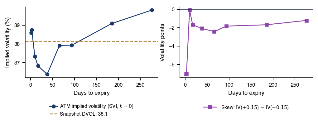
The mean of the VIX is 19.4, which corresponds to 5.6% a month. The range runs from 9.1 to 82.7; the maximum was reached on 16 March 2020, during the COVID-19 crisis. The VIX was above 30 on 7.9% of days. Its peaks are sudden spikes followed by slow decay, as in the GARCH models of Chapter 5. The term structure of implied volatility is in Further Topics.
In brief
Daily close; the six highest peaks at least 500 days apart are labelled
Mean \(19.4\) (\(5.6\%\) a month), range \(9.1\)–\(82.7\) (2020-03-16, COVID-19)
above 30 on \(7.9\%\) of days
sudden spikes, slow decay, as in GARCH (Chapter 5)
The variance risk premium (VRP) is the difference between the variance priced by options and the variance expected by investors, as defined by Carr & Wu (2009) and Bollerslev, Tauchen & Zhou (2009). Three versions must not be confused. The economic, ex-ante premium is \(E^Q_t[RV_{t,t+21}] - E^P_t[RV_{t,t+21}]\), where \(P\) is the real-world measure; \(VIX_t^2\) estimates the first term, while the second needs a forecast. The ex-post premium, used in this section,
is the realised P&L of the seller of a variance swap and is known only at \(t + 21\). The ex-ante proxy, \(VIX_t^2 - RV_{t-21,t}\), uses past variance as the forecast of \(E^P_t\); it is known at \(t\), so it can serve as a predictor (Section 11).
In (12.17),\(r_{t+i}\) are the daily log returns in %, so \(RV\) is annualised and measured in %\(^2\), like \(VIX^2\). The 21 trading days cover roughly the same month as the 30 calendar days of the VIX. The premium is positive on average if investors dislike states with high volatility, which are also bad states for their wealth.
The windows of consecutive days overlap by 20 of 21 days, so the series (12.17) is autocorrelated by construction. The standard error of its mean needs Newey–West with at least 21 lags (Newey & West, 1987). Twenty-one lags cover the overlap but not the persistence of volatility, so the sensitivity to longer bandwidths is reported: the standard error of the premium, in volatility points, is 0.27 with 21 lags, 0.31 with 42, 0.32 with 63 and 0.33 with 126.
The interactive chart has two panels. The upper panel shows the VIX and the volatility realised over the next 21 trading days, \(\sqrt{RV_{t,t+21}}\), in annualised %. The lower panel shows their difference, the ex-post premium in volatility points. The slider moves the start of the sample, and the ▶ button moves it forward year by year, so that the reader can see whether the mean premium depends on the early years.
Question for the room On what share of days is the VIX above the volatility realised over the next 21 trading days?
Answer
On approximately 86% of days; 14% corresponds to the opposite event. An unbiased forecast does not automatically imply a 50% exceedance frequency. Over the full sample, the mean premium is 4.09 volatility points (Newey–West standard error 0.27), or 113 %² in variance, with t = 5.5. Negative values occur when subsequent realised volatility exceeds VIX; the largest losses occur during stress episodes: the worst window, starting on 20 February 2020, has −72.0 points. From 2020, the mean volatility difference is 3.82 points, with Newey–West SE (Standard Error) 0.90 and t = 4.25. The mean variance difference is 73.90 %², with SE 79.90 %² and t = 0.92.
Over the whole sample the VIX lies above the realised volatility most of the time, and the premium becomes negative mainly in crises. The numbers are on the next slide.
The sample has 9,203 days from 1990 to 2026. The mean VIX is 19.4 and the mean realised volatility over the next 21 trading days 15.3. The premium is 4.09 volatility points, with a Newey–West standard error (SE) of 0.27. In variance units it is 113 %\(^2\), with \(t = 5.5\); the \(t\)-statistic in variance requires a finite fourth moment of returns, which Chapter 1 questions.
The premium is positive on 86% of days. The exceptions are crashes: the worst value, \(-72.0\) volatility points, belongs to the window that starts on 20 February 2020, at the beginning of the COVID-19 crisis.
The message is the same as for the delta-hedged option of Section 5: sellers of volatility are paid on average and lose in crises. The result is a description of an ex-post premium. The economic premium needs a forecast of \(E^P_t\) (slide The Variance Risk Premium).
In brief
Top: VIX and the volatility realised over the next 21 trading days
bottom: their difference VIX \(-\) RV, 1990–2026
here RV \(= \sqrt{RV_{t, t + 21}}\), the realised volatility, in vol points
9 203 days: mean VIX \(19.4\), mean realised \(15.3\)
Premium \(4.09\) vol points (Newey–West standard error, SE, \(0.27\)); in variance, \(113\) %\(^2\), \(t = 5.5\)
the \(t\) in variance requires a finite fourth moment, which Chapter 1 questions
Positive on \(86\%\) of days
the exceptions are crashes
Worst \(-72.0\) vol points, window from 2020-02-20 (COVID-19)
Same message as the delta-hedged option
sellers of volatility are paid on average and lose in crises
Type of evidence: description
an ex-post premium; the economic premium needs a forecast of \(E^P_t\) (slide The Variance Risk Premium)
An unbiased forecast has \(\alpha = 0\) and \(\beta = 1\). The standard errors are Newey–West with 21 lags, because the targets overlap. Inference on the coefficients needs a finite second moment of the regression score \(x_t u_t\) and weak dependence; in variance units this means eighth moments of returns, which Chapter 1 questions.
The interactive chart plots the realised volatility over the next 21 days against the VIX at day \(t\), both in %, with the 45-degree line on which realised equals implied and the Mincer–Zarnowitz fit, estimated in variance and drawn back in volatility. The slider keeps only the days with the VIX up to a chosen level, and the ▶ button moves this cut-off, which shows how much the high-volatility days weigh in the fit.
Question for the room In the regression of realised variance on VIX², the separate tests do not reject α = 0 and β = 1. What can we conclude from these two results alone?
Answer
The separate tests do not determine the joint test’s result. Here, the estimates have correlation −0.90 and both deviations from the null are negative (α̂ = −51.9, β̂ − 1 = −0.14). Using this covariance, the Wald test gives χ²₂ = 41.7 and p ≈ 8.9·10⁻¹⁰. The VIX explains R² = 0.37 of the subsequent realised variance, past realised variance only 0.29.
The estimates are \(\hat\alpha = -51.9\) (SE 34.4) and \(\hat\beta = 0.860\) (SE 0.105), with \(R^2 = 0.37\). Separately, neither coefficient differs significantly from its null value: \(t = -1.51\) for \(\alpha = 0\) and \(t = -1.34\) for \(\beta = 1\). But the two estimates have a correlation of \(-0.90\) and both deviate downwards, so the joint Wald test rejects unbiasedness: \(\chi^2_2 = 41.7\),\(p = 8.9 \cdot 10^{-10}\). On the chart, most points lie below the 45-degree line.
Past realised variance alone explains less, with \(R^2 = 0.29\). With both regressors, the VIX keeps its weight, 0.77, and past variance adds little, 0.08 with SE 0.13. Regressions in logs, with instruments and against the HAR-RV (Heterogeneous AutoRegressive model of Realised Volatility) model are in Further Topics.
inference on coefficients needs \(E\|x_t\varepsilon_t\|^2 < \infty\) (\(x_t\): the regressors) and weak dependence; in variance units, eighth moments of returns, which Chapter 1 questions
The VIX is the discrete version of the variance strip (12.15). On the S&P 500 in 1990–2026 it exceeds the volatility realised over the next 21 days by 4.09 points on average, with a Newey–West standard error of 0.27, and the premium is negative mainly in crashes. As a forecast of next month's variance it is biased in levels, by the joint Wald test, but past variance adds little to it.
Options with Zero Days to Expiry
Options that expire on the day they are traded have become a large part of the index-option market. This section summarises the evidence on these contracts and shows, with the Black–Scholes Greeks, what happens to gamma and time decay in the last day.
0DTE options, with zero days to expiry, are options traded on the day they expire. S&P 500 options now expire every trading day, so a contract with zero days to expiry is listed on every trading day.
Beckmeyer, Branger & Gayda (2023) report that more than 75% of retail trades in S&P 500 options involve 0DTE contracts, and that retail investors lose money on them. Brogaard, Han & Won (2023) find that 0DTE options were 48% of index-option trading in August 2023 and that more 0DTE trading is followed by higher index volatility, mostly through speculative retail trades.
Pricing at ultra-short horizons needs corrections for skewness and kurtosis (Bandi, Fusari & Renò, 2023). The Greeks of Section 4 already show the main effect: as \(\tau \to 0\), gamma and theta explode at the money.
In brief
0DTE options are traded on the day they expire Cboe (2023)
The interactive chart has two panels. The left panel shows the gamma of a call with \(K = 100\) as a function of the price \(S\), for the number of trading days to expiry chosen with the first slider. The right panel shows the time decay of an at-the-money call, \(-\Theta\) per calendar day, against the number of calendar days to expiry, with the axis reversed so that expiry is on the right. The second slider sets the volatility \(\sigma\), and the ▶ button moves towards expiry.
Question for the room How much larger is the ATM gamma one trading day before expiry than one month before?
Answer
At S = K = 100, r = 0 and σ = 16%, gamma is 0.396 for τ = 1/252 and 0.086 for τ = 21/252. The ratio is approximately √21 ≈ 4.6: the φ(d₁) factor changes very little here. A 1% move in the last day changes delta by about 0.4; the relation dΔ ≈ Γ·dS is a local approximation. The values 0.167 and 0.030 are −theta per calendar day, evaluated with one and 30 calendar days remaining.
At \(S = K = 100\),\(\sigma = 16\%\) and \(r = 0\), the ATM gamma one day before expiry is 0.396, against 0.086 one month before. The numbers are discussed on the next slide.
The left panel compares the gamma of a call with \(K = 100\) one day, one week and one month before expiry; the right panel shows the daily time decay of an ATM call. The inputs are \(S = K = 100\),\(\sigma = 16\%\) and \(r = 0\). Gamma counts trading days, \(\tau = 1/252\) and \(21/252\), and time decay counts calendar days, \(\tau = 1/365\) and \(30/365\), as on the two axes.
At the money, \(\Gamma = \varphi(d_1)/(S\sigma\sqrt{\tau})\) with \(d_1\) close to zero, so gamma grows like \(1/\sqrt{\tau}\). One day before expiry it is 0.396, against 0.086 one month before: 4.6 times larger, \(\sqrt{21}\). A 1% move in the last day therefore changes delta by about 0.4.
Time decay grows in the same way. It is 0.167 in the last day, against 0.030 with 30 days left, about 5.5 times more. The ATM value of the call, about \(0.4\,S\sigma\sqrt{\tau} = 0.33\), is lost entirely during that day, roughly twice the starting rate. The seller of a 0DTE option collects fast decay and carries a large gamma risk. A stylised test of selling same-day straddles is in Further Topics.
In brief
Left: gamma of a call with \(K = 100\) one day, one week and one month before expiry
gamma counts trading days (\(\tau = 1/252\) and \(21/252\))
time decay counts calendar days (\(\tau = 1/365\) and \(30/365\)), as on the two axes
ATM gamma one day before expiry \(0.396\) vs \(0.086\) one month before
\(4.6\) times larger (\(= \sqrt{21}\))
a 1% move in the last day changes delta by about 0.4
Time decay \(0.167\) in the last day vs \(0.030\) with 30 days left
about \(5.5\) times more
the seller collects fast decay and carries large gamma risk
The ATM value with one day left, about \(0.4\,S\sigma\sqrt{\tau} = 0.33\), is lost entirely during that day: twice the decay rate at the start of the day (\(0.167\))
As expiry approaches, ATM gamma grows like \(1/\sqrt{\tau}\): in the last day it is \(\sqrt{21} \approx 4.6\) times its value one month before. The seller of a 0DTE option earns fast time decay and carries the largest gamma risk of any maturity.
Case Studies: Option-Implied Bounds and Volatility Expectations
The two case studies use option prices as information about expected returns and expected variance:
Back, Crotty & Kazempour (2022) test whether lower bounds on the equity premium computed from option prices are valid, tight and useful for forecasting.
Lochstoer & Muir (2022) ask whether the VIX reacts too slowly to volatility shocks; the case study replicates their main regression on the course data.
Back, Crotty & Kazempour (2022) study lower bounds on the equity premium obtained from option prices. They ask three questions. Are these bounds valid conditionally, that is, does the expected excess return exceed the bound at each date? Are they tight conditionally, that is, is the expected excess return equal to the bound? Do they forecast returns out of sample?
A tight bound would be a real-time forecast of the equity premium with no estimated parameter. The usual test regresses realised returns on the bound. Martin (2017) could not reject \(\alpha = 0\) and \(\beta = 1\) in this regression on 1996–2012, but the test has low power, because realised returns are very noisy relative to the bound.
where \(R_{t,T}\) is the gross market return, \(R_{f,t,T}\) the gross riskless return and \(\mathrm{var}^Q_t\) the risk-neutral variance; here \(\mathrm{SVIX}^2_{t,T}\) is not annualised. The bound is valid if \(\mathrm{cov}_t(M_{t,T}R_{t,T}, R_{t,T}) \le 0\), where \(M_{t,T}\) is the stochastic discount factor, and tight if this covariance is zero, for example for a log-utility investor who holds the market.
The Chabi-Yo–Loudis bound (Chabi-Yo & Loudis, 2020) is built from the first four risk-neutral moments. In its restricted form it is free of preference parameters.
The link to this chapter is static spanning: SVIX is the strip (12.2) with \(f = S^2\) (Appendix). The paper works with the realised slackness \(s_{t,T} = R^e_{t,T} - b_{t,T}\), the excess return minus the bound \(b_{t,T}\). Validity means \(E_t[s_{t,T}] \ge 0\) and tightness means \(E_t[s_{t,T}] = 0\).
In brief
Martin bound (eq. 3):
\(R_{t,T}\) the gross market return, \(R_{f,t,T}\) the gross riskless return
\(\mathrm{var}^*_t\) the risk-neutral variance (\(\mathrm{SVIX}^2_{t,T}\) not annualised here)
Valid if \(\mathrm{cov}_t(M_{t,T}R_{t,T}, R_{t,T}) \le 0\) (\(M_{t,T}\) the stochastic discount factor); tight if this covariance is zero, e.g. a log-utility investor who holds the market
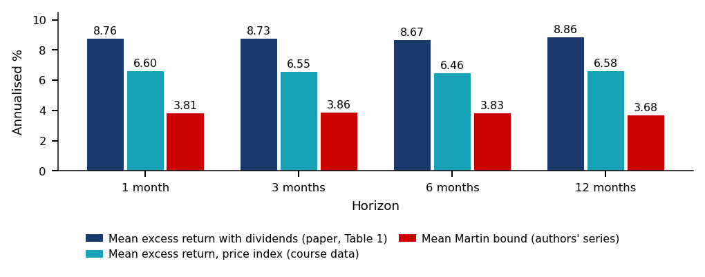
The data are described in Section 3 and Appendix C of the paper; the option filters are in the Appendix. The bounds of Martin and of Chabi-Yo and Loudis are computed daily, from January 1990 to December 2020, from S&P 500 index options, and interpolated to 30, 90, 180 and 360 days. The returns are S&P 500 excess returns over 21, 63, 126 and 252 trading days, annualised, in %. They are compounded as \(\prod(1 + r - r_f) - 1\), the convention of the authors' code, which differs from \(\prod(1 + r) - \prod(1 + r_f)\).
Conditional validity is tested through unconditional moments (eq. 10):
\[E\big[(R^e_{t,T} - b_{t,T})\,z_t\big] \ge 0\]
for any nonnegative variable \(z_t\) known at \(t\). The instruments \(z_t\) are a constant and nine predictors of Welch & Goyal (2008), transformed to be positive (Table 3). If the bound holds conditionally, each of these ten moments is nonnegative.
Forecasting uses predictive regressions with the bias correction of Amihud & Hurvich (2004) (Tables 5 and 6). A persistent predictor biases the ordinary least squares (OLS) slope, the Stambaugh bias, so the innovation of the predictor, estimated from a bias-corrected first-order autoregression, is added as a regressor. Out of sample, monthly forecasts are compared with the historical mean through \(R^2_{OS}\), the out-of-sample \(R^2\) against that mean (Table 8); the protocol is in the Appendix.
Amihud–Hurvich: a persistent predictor biases the OLS (Ordinary Least Squares) slope (Stambaugh bias), so the innovation of the predictor, estimated from a bias-corrected AR(1), is added as a regressor
Monthly out-of-sample forecasts against the historical mean
measured by \(R^2_{OS}\), the out-of-sample \(R^2\) against that mean
The moment inequalities are tested jointly with the statistics of Kodde & Palm (1986) (eqs. 11–14 of the paper). Let \(\bar\lambda\) be the vector of the 10 sample means of the moments and \(\Sigma\) their covariance, estimated with the method of Hansen & Hodrick (1980) with as many lags as days in the horizon. The Hansen–Hodrick covariance keeps, with equal weights, exactly the autocovariances created by the overlap of the return windows.
Validity, \(H_0\):\(\lambda_0 \ge 0\), is tested by the distance from \(\bar\lambda\) to the region in which all moments are nonnegative, and tightness, \(H_0\):\(\lambda_0 = 0\) against \(\lambda_0 \ge 0\), by the remaining part of the Wald statistic:
\(D_1\) is zero if all sample moments are already positive. A large \(D_2\) rejects tightness.
A two-moment example with \(\Sigma = I\) shows the mechanics. With \(\bar\lambda = (0.5, -0.2)\), the closest point with nonnegative coordinates is \((0.5, 0)\), so \(D_1 = 0.2^2 = 0.04\) and \(D_2 = 0.29 - 0.04 = 0.25\). With \(\bar\lambda = (0.5, 0.2)\),\(D_1 = 0\) and \(D_2 = 0.29\).
Under \(H_0\) some inequality constraints bind and others do not, so the statistics do not have a single \(\chi^2\) distribution. Both follow weighted mixtures of \(\chi^2_0, \dots, \chi^2_{10}\), and Kodde & Palm (1986) tabulate bounds on the critical values.
In brief
Kodde & Palm (1986) (eqs. 11–14): \(\bar\lambda\) is the vector of the 10 sample means
The table reports, for each horizon, the mean excess return \(R^e\) and the mean Martin bound \(b\), both in % a year, the Kodde–Palm statistics \(D_1\) and \(D_2\), the forecasting slope \(\hat\beta\) with its standard error and the out-of-sample \(R^2_{OS}\), all from Back, Crotty & Kazempour (2022).
Validity is not rejected: \(D_1 = 0\) and the \(p\)-value is 100% at every horizon, because all 10 sample moments are positive. This does not prove that the bound is valid in every state; it means that the data contain no evidence against validity for these moments.
The bound is not tight. \(D_2\) exceeds 28.86, the upper 0.1% Kodde–Palm critical value for 10 restrictions, at every horizon. The finite-sample \(p\)-values are 3.6%, 0.4%, 2.6% and 8.3% at 1, 3, 6 and 12 months. The mean slackness is 4.8 to 5.2 points a year, so the bound is less than half of the realised premium. The evidence concerns mean slackness over 1990–2020, not forecasting power: out of sample the bound loses to the historical mean (Further Topics).
The same statistic \(D_2\) is read against two yardsticks. The asymptotic critical value rejects tightness at every horizon. The finite-sample \(p\)-values reject at 5% at 1, 3 and 6 months, but not at 12 months, where \(p = 8.3\%\).
With a Holm correction for the four horizons (Section 11), the finite-sample test rejects only at 3 months. The smallest \(p\)-value, 0.4%, is below \(5\%/4 = 1.25\%\), but the next one, 2.6%, is above \(5\%/3 = 1.67\%\), and the procedure stops. The asymptotic test rejects at every horizon even after the correction.
The tests can disagree because \(\Sigma\) is imprecise. The years 1990–2020 hold only about 31 non-overlapping 12-month windows, and the moments use persistent predictors, so asymptotic critical values can be too small. The finite-sample \(p\)-value is the more cautious reading. Both should be reported, never only the one that rejects (Seminar 12, C3).
The economic conclusion does not depend on the test. The mean slackness of 4.8–5.2 points a year means that the bound covers less than half of the realised premium at every horizon.
In brief
Same \(D_2\), two yardsticks
the asymptotic critical value rejects tightness at every horizon
the finite-sample \(p\)-values reject at 5% at 1, 3 and 6 months, but not at 12 months
With a Holm correction for four horizons (Section 11), the finite-sample test rejects only at 3 months
Holm compares the smallest \(p\) with \(5\%/4\), the next with \(5\%/3\): \(0.4\% < 1.25\%\), then \(2.6\% > 1.67\%\), so it stops
The asymptotic test rejects at every horizon even after the correction
Why they can disagree: \(\Sigma\) is imprecise
1990–2020 holds only about 31 non-overlapping 12-month windows
the moments use persistent predictors
so asymptotic critical values can be too small
The finite-sample \(p\) is the more cautious reading
report both, never only the one that rejects (Seminar 12, C3)
The mean slackness of 4.8–5.2 points a year does not depend on the test
economically, the bound covers less than half of the realised premium at every horizon
Case Study: the Bound and the Realised Premium (1/2)
The interactive chart has two panels. The upper panel shows the authors' daily 1-month bounds, Martin (SVIX) and Chabi-Yo–Loudis, from 1990 to 2020, in annualised %, from the replication package. The lower panel uses the course data: the realised excess return of the S&P 500 price index over the horizon chosen with the slider, compared with the Martin bound of the same horizon, with the dates on which the realised return falls below the bound marked. The ▶ button steps through the horizons of 1, 3, 6 and 12 months.
Question for the room The realised 12-month excess return is below the Martin bound on 33% of dates. Does this contradict the validity of the bound?
Answer
No. The bound restricts the conditional mean Eₜ[Rᵉ], not each realised return. D₁ = 0 at all horizons means that the test does not reject validity; it does not prove it. For tightness, the asymptotic tests reject, but the finite-sample p-value at 12 months is 8.3%, so that test does not reject at 5%. Mean slackness at 12 months is approximately 5.18 percentage points a year in the paper, including dividends, and 2.91 for the price index in the figure. The correlation between the bound and the realised return is only 0.15.
The 1-month bound has a median of 2.7% and a peak of 54.4% on 16 March 2020; the 12-month bound peaks at 21.1% on 20 November 2008. The numbers are discussed on the next slide.
The upper panel shows the authors' daily 1-month bounds for 1990–2020. The lower panel, on the course data, shows the 12-month excess return of the S&P 500 price index together with the 12-month Martin bound. The 1-month bound has a median of 2.7% and a peak of 54.4%, on 16 March 2020; the 12-month bound peaks at 21.1%, on 20 November 2008. Being a risk-neutral variance, the bound jumps with the VIX in crises.
The Chabi-Yo–Loudis bound is at or above the Martin bound on 99.99% of days. It uses the higher risk-neutral moments, and negative skewness and fat tails raise it.
The realised 12-month excess return lies below the bound on 33% of dates, mainly in 2000–2002 and 2007–2008. This is no contradiction: the bound restricts the conditional mean \(E_t[R^e_{t,T}]\), not each realisation. The correlation between the bound and the realised return is 0.15, computed on overlapping windows and therefore descriptive only. Return noise dwarfs the variation of the bound, which explains the imprecise slopes and the negative \(R^2_{OS}\) of the paper.
The replication, exercise C3 of Seminar 12, uses the authors' daily bound series from the replication package, the daily S&P 500 closes of the course data, the daily risk-free rate of the Kenneth French Data Library and the Welch–Goyal predictors from Amit Goyal's data page. It rebuilds Table 1 and the statistics \(D_1\) and \(D_2\) of Table 3.
The authors state three limitations. The series starts in 1990 because the bounds need option prices, so the out-of-sample tests have little power (Section 6 of the paper). Validity holds even when the bound is replaced by its time-series mean, so validity says nothing about predictive power (Section 4.3). More recent bounds and formulas for risk premia are not tested (Introduction). An open extension of the case study is in Further Topics.
Lochstoer & Muir (2022) argue that investors update their expectations of market volatility too slowly: after a volatility shock they first underreact and later overreact. The question matters for the VRP. \(VIX^2\) is the risk-neutral price of 30-day variance, and the VRP is \(VIX^2\) minus the objective expected variance \(\hat\sigma^2_t\). If the VIX rises less than expected variance, the VRP falls exactly when risk rises.
The paper models the market's expectation as a weighted average of past realised variance (equation 4):
\[\mathrm{VIX}^2_t = a + b \sum_{j=0}^{11} \phi^j\, rv_{t-j} + \varepsilon_t,\]
(12.21)
where \(rv_t\) is the realised variance of month \(t\), the annualised sum of squared daily S&P 500 log returns. With \(\phi = 0\) only the current month counts; a larger \(\phi\) means expectations that move more slowly.
In the paper (Section I), \(\phi = 0.42\) with standard error 0.12 for \(VIX^2\), from January 1990 to April 2020. After a shock to expected variance, the response of the VRP is negative at first and changes sign after the third month (Figure 2). The authors propose that this explains a weak risk–return tradeoff: the premium rises only once volatility has started to fall.
In brief
Lochstoer & Muir (2022): investors update their expectations of market volatility too slowly
underreaction first, after a volatility shock, then delayed overreaction
Why it matters: VIX\(^2\) is the risk-neutral price of 30-day variance
if the VIX rises less than expected variance, the VRP (variance risk premium) falls exactly when risk rises
VRP \(=\) VIX\(^2\) minus the objective expected variance \(\hat\sigma^2_t\)
The market's expectation as a weighted average of the past (equation 4 of the paper): \(\mathrm{VIX}^2_t = a + b \sum_{j=0}^{11} \phi^j\, rv_{t-j} + \varepsilon_t\)
\(rv_t\): realised variance of month \(t\), the sum of squared daily S&P 500 log returns, annualised
\(\phi = 0\): only the current month counts; a larger \(\phi\) means expectations that move more slowly
The paper's numbers (Journal of Finance, Section I): \(\phi = 0.42\) (standard error \(0.12\)) for VIX\(^2\), January 1990 to April 2020
after a shock to expected variance, the VRP response is negative at first and changes sign after the third month (Figure 2)
The consequence the authors propose: a weak risk–return tradeoff, because the premium rises only once volatility has started to fall
How the VIX Responds to a Shock to Expected Variance
The left panel shows the monthly responses, in annualised %\(^2\), to a one-standard-deviation shock to the expected variance \(\hat\sigma^2\), estimated with a vector autoregression (VAR) on 1992–2026: the response of expected variance, of \(VIX^2\) and of the VRP, with a 95% bootstrap band for the VRP. The right panel shows the weights \(\hat\phi^{\,j}\) of (12.21) on the variance of month \(t - j\), for \(VIX^2\) and for next month's realised variance. The slider sets the last year of the sample, and the ▶ button extends it from 2005 to 2026.
The identity behind the left panel is \(VIX^2 = \) expected variance \(+\) VRP. If \(VIX^2\) rises by less than the shock to expected variance, the VRP must fall on impact.
Question for the room Keep the same Cholesky ordering, with expected variance first. Press ▶ to extend the sample from December 2005 to August 2026. How does the sign of the impact response of the VRP change?
Answer
The point estimate is negative in every sample: −69 %² up to 2005, −254 %² up to 2008. The pointwise 95% band includes zero only for the sample ending in 2006. In the full sample, the response is −169 %², with a band of [−300, −27]: VIX² rises by only 55% of the shock to expected variance. The VRP response turns positive from month 2 and peaks in month 3 (+30 %²). The weights point the same way: φ̂ = 0.49 for VIX², against 0.11 for next month's realised variance. The result is conditional on the Cholesky ordering and the estimated HAR (Heterogeneous AutoRegressive, model) series; it does not by itself establish a trading rule or identify slow-moving expectations.
On the full sample, a shock of 375 %\(^2\) to \(\hat\sigma^2\) raises \(VIX^2\) by only 206 %\(^2\), 55% of the shock. The VRP responds with \(-169\) %\(^2\) on impact, becomes positive from month 2 and reaches \(+30\) in month 3. The estimates and their limits are on the following slides.
In brief
Left: the monthly response, in annualised %\(^2\), to a one-standard-deviation shock to \(\hat\sigma^2\) in a vector autoregression (VAR), 1992–2026
Right: the weights \(\hat\phi^{\,j}\) on the variance of month \(t-j\), for VIX\(^2\) and for next month's realised variance
In the paper, \(\phi\) is estimated from (12.21) for \(VIX^2\) and, as the rational benchmark, for subsequent realised variance. The expected variance \(\hat\sigma^2_t\) is the real-time forecast of next month's variance from a HAR (heterogeneous autoregressive) model on 5-minute returns. Table III regresses next month's variance and \(VIX^2\) on \(\hat\sigma^2_t\) and on a weighted average of the last 6 values of \(\hat\sigma^2\), with weights proportional to \(0.5^j\). A monthly VAR(1), a first-order vector autoregression, with \(\hat\sigma^2\) ordered first in a Cholesky decomposition, gives the responses to the shock.
The course replication uses daily S&P 500 and VIX data from January 1990 to August 2026, 440 months. The expected variance \(\hat\sigma^2_t\) comes from a HAR model on daily returns, with the last day, the last 5 days and the last 21 days as regressors, re-estimated each month on the data available then. The first 24 months are the burn-in, so \(\hat\sigma^2\) starts in January 1992. The VAR has three variables: \(\hat\sigma^2\), the VRP and the excess return of the price index, with the risk-free rate from Kenneth French. The paper adds the log price–dividend ratio, which is not in the course data.
The standard errors of \(\hat\phi\) come from a moving block bootstrap with 18-month blocks, like the paper's 6 quarters. Table III uses Newey–West standard errors with 12 lags, and the VAR bands come from a residual bootstrap. The heteroskedasticity and autocorrelation consistent (HAC) standard errors need \(E\|x_t u_t\|^2 < \infty\) and weak dependence; with \(x_t\) and \(u_t\) in variance units, this means eighth moments of returns, which Chapter 1 questions.
In brief
The paper: \(\phi\) estimated from equation 4 for VIX\(^2\) and, as the rational benchmark, for subsequent realised variance
\(\hat\sigma^2_t\): the real-time forecast of next month's variance, a HAR (heterogeneous autoregressive) model on 5-minute returns
Table III: regressions on \(\hat\sigma^2_t\) and on the weighted average of the last 6 values of \(\hat\sigma^2\), with weights proportional to \(0.5^{j}\)
a monthly VAR(1) with \(\hat\sigma^2\) ordered first (Cholesky) gives the responses to the shock
The course replication: daily S&P 500 and VIX, January 1990 to Aug 2026 (440 months)
\(\hat\sigma^2_t\): HAR on daily returns (last day, last 5 and last 21 days), re-estimated each month on the data available then
the first 24 months are the burn-in, so \(\hat\sigma^2\) starts in January 1992
the VAR has three variables: \(\hat\sigma^2\), the VRP and the excess return of the price index (risk-free rate: Kenneth French)
the paper adds the log price–dividend ratio, not in the course data
Inference
standard errors of \(\hat\phi\): moving block bootstrap with 18-month blocks, like the paper's 6 quarters
Table III: Newey–West standard errors with 12 lags; VAR bands: residual bootstrap
HAC (Heteroskedasticity and Autocorrelation Consistent) standard errors such as Newey–West need \(E\|x_tu_t\|^2 < \infty\) (\(x_t\): regressors, \(u_t\): errors) and weak dependence; in variance units, eighth moments of returns, which Chapter 1 questions
The VIX Depends More Persistently on Past Variance
The estimated weight \(\hat\phi\) in (12.21) is 0.54 for \(VIX^2\) (standard error 0.08) on the paper's sample and 0.49 (0.08) up to 2026. For next month's realised variance it is 0.26 (0.30) and 0.11 (0.20), not significantly different from zero. The VIX thus puts more weight on past variance than realised variance does.
Table III on 334 months, 1992–2020, points the same way. Next month's variance depends on \(\hat\sigma^2_t\), with coefficient 0.82 (s.e. 0.12), and the coefficient of the past average is not significant, 0.04 (s.e. 0.10); the paper (Panel A, column 6) reports 1.53 (0.54) and \(-0.58\) (0.46). \(VIX^2\) depends on both: 0.56 (0.09) and 0.41 (0.04), with \(R^2 = 0.79\), against 0.30 (0.12) and 0.64 (0.07), with \(R^2 = 0.79\), in the paper (Panel A, column 7). In the VAR, a shock of 375 %\(^2\) to \(\hat\sigma^2\) raises \(VIX^2\) by only 206 %\(^2\), 55% of the shock. The VRP responds with \(-169\) %\(^2\) on impact, with a pointwise 95% band of \([-300, -27]\), becomes positive from month 2 and reaches \(+30\) in month 3.
The result is a description consistent with slow expectations, on daily instead of 5-minute data. It does not identify the mechanism: a rationally time-varying price of variance risk could give the same signs. The daily HAR forecasts less well than the paper's model, with \(R^2 = 0.32\) for next month's variance against 0.47, and part of the weight the VIX puts on the past may be information that the daily HAR lacks. Months of very high variance, in 2008 and 2020, dominate the regressions in levels, and the Cholesky ordering changes the initial sign of the response (next slide).
In brief
Replication: \(\hat\phi\) for VIX\(^2\) is \(0.54\) (standard error \(0.08\)) on the paper's sample (paper: \(0.42\)), \(0.49\) (\(0.08\)) up to 2026
for next month's realised variance: \(0.26\) (\(0.30\)) and \(0.11\) (\(0.20\)), not significantly different from zero
Table III, 334 months, 1992–2020: next month's variance depends on \(\hat\sigma^2_t\) (\(0.82\), s.e. \(0.12\)); the past-average coefficient is not significant (\(0.04\), s.e. \(0.10\))
in the paper (Panel A, column 6): \(1.53\) (\(0.54\)) and \(-0.58\) (\(0.46\))
VIX\(^2\) depends on both: \(0.56\) (\(0.09\)) and \(0.41\) (\(0.04\)), \(R^2 = 0.79\)
in the paper (Panel A, column 7): \(0.30\) (\(0.12\)) and \(0.64\) (\(0.07\)), \(R^2 = 0.79\)
VAR: a shock of \(375\) %\(^2\) to \(\hat\sigma^2\) raises VIX\(^2\) by only \(206\) %\(^2\) (\(55\%\) of the shock)
VRP response: \(-169\) %\(^2\) on impact (pointwise \(95\%\) band: \([-300, -27]\)), positive from month 2, \(+30\) in month 3
Type of evidence: a description consistent with slow expectations, on daily instead of 5-minute data
it does not identify the mechanism: a rationally time-varying price of variance risk could give the same signs
The limits
the daily HAR forecasts less well: \(R^2 = 0.32\) for next month's variance, against \(0.47\) in the paper
part of the VIX weight on the past may be information our HAR lacks
months of very high variance (2008, 2020) dominate the regressions in levels; the Cholesky ordering changes the initial sign (next slide)
The difference \(\hat\phi_{\mathrm{VIX}} - \hat\phi_{RV}\) is bootstrapped on the same 18-month blocks for both regressions. On the paper's sample it is 0.29, with a 95% interval of \([-0.05, 0.91]\), so the difference is not significant at 5%. Up to 2026 it is 0.38, with interval \([0.08, 0.80]\), significant at 5%.
The VAR bands are conditional on the estimated \(\hat\sigma^2\) series. The bootstrap resamples the VAR residuals without re-estimating the first-stage HAR, and the bands are pointwise, horizon by horizon, not simultaneous over all horizons. The Newey–West errors of Table III also leave out the uncertainty of \(\hat\sigma^2\).
The VAR(1) is stable: the largest eigenvalue has modulus 0.73. The return residuals are conditionally heteroskedastic (Engle test with 12 lags, \(p < 0.001\)), so resampling the residuals independently is only an approximation.
The Cholesky ordering matters. With \(\hat\sigma^2\) ordered last, the VRP response is 0 on impact, by construction, and \(+33\) %\(^2\) in month 1. The negative initial sign rests on the assumption that \(\hat\sigma^2\) does not respond within the month to VRP shocks.
In brief
The difference \(\hat\phi_{\mathrm{VIX}} - \hat\phi_{RV}\): bootstrap on the same 18-month blocks for both regressions
paper's sample: \(0.29\), 95% interval \([-0.05, 0.91]\), so the difference is not significant at 5%
up to 2026: \(0.38\), 95% interval \([0.08, 0.80]\), significant at 5%
The VAR bands are conditional on the estimated \(\hat\sigma^2\) series
the bootstrap resamples the VAR residuals without re-estimating the first-stage HAR
the bands are pointwise, horizon by horizon, not simultaneous over all horizons
the Newey–West errors of Table III also leave out the uncertainty of \(\hat\sigma^2\)
VAR(1) diagnostics
stable: the largest eigenvalue has modulus \(0.73\)
the return residuals are conditionally heteroskedastic (Engle test, 12 lags, \(p < 0.001\))
resampling the residuals independently is therefore only an approximation
The Cholesky ordering matters
with \(\hat\sigma^2\) ordered last, the VRP response is 0 on impact, by construction, and \(+33\) %\(^2\) in month 1
the negative initial sign rests on \(\hat\sigma^2\) not responding within the month to VRP shocks
Section summary
The results of the two case studies:
The option-implied bounds on the equity premium are not rejected as valid and are not tight in 1990–2020: they cover less than half of the realised premium, and out of sample they do not beat the historical mean.
On the course data, \(VIX^2\) puts more weight on past variance than realised variance does, and the VRP falls on impact after a shock to expected variance.
Both results are descriptions that depend on test choices: the critical values and the Holm correction in the first, the Cholesky ordering and the first-stage HAR in the second.
AI for Scientific Discovery
This section states an open question of the chapter as a testable hypothesis: does the variance risk premium of Section 8 still predict equity returns after 2007? It gives the inference tools the question requires, the checks a researcher must run on the output of an AI assistant, a mini-case on the course data and a project idea.
The question is whether the VRP still predicts equity returns after 2007. Answering it requires three tools:
For overlapping returns, Hodrick 1B standard errors (Hodrick, 1992). They keep the regression of overlapping \(h\)-month returns on \(\mathrm{VRP}_t\) and change only the covariance estimator of the coefficient. Its score is the one-month residual under \(H_0\) times the sum of the last \(h\) values of the regressor, so the covariance needs no autocovariances of overlapping errors.
For out-of-sample evaluation, the Clark–West test (Clark & West, 2007).\(R^2_{OS} > 0\) means that the predictive model has a lower mean squared forecast error than the historical mean. For nested models, the Clark–West test tests this; it adjusts for the noise that estimating a truly zero slope adds to the larger model, which otherwise penalises the predictive model under the null.
For \(m\) tests, for example four horizons, the Holm correction. The \(p\)-values are sorted; the smallest is compared with \(\alpha/m\), the next with \(\alpha/(m - 1)\), and so on, and the procedure stops at the first that fails. With \(p = 0.01\), 0.03 and 0.04, \(\alpha = 0.05\) and \(m = 3\), the first comparison, \(0.01 < 0.0167\), rejects, and the second, \(0.03 > 0.025\), stops the procedure. Only one hypothesis is rejected, although all three \(p\)-values are below 0.05.
In brief
The section's question: does the VRP (Section 8) still predict equity returns after 2007?
Hodrick 1BHodrick (1992): keep the regression of overlapping \(h\)-month returns on \(\mathrm{VRP}_t\)
only the covariance estimator of the coefficient changes
its score: the one-month residual under \(H_0\) times the sum of the last \(h\) values of the regressor
so the covariance needs no autocovariances of overlapping errors
\(R^2_{OS} > 0\): the predictive model beats the historical mean
lower mean squared forecast error than the historical mean
it adjusts for the noise that estimating a truly zero slope adds to the larger model
Holm correction for \(m\) tests (e.g. four horizons)
sort the \(p\)-values
compare the smallest with \(\alpha/m\), the next with \(\alpha/(m - 1)\), and so on
stop at the first that fails
Example: \(p = 0.01, 0.03, 0.04\), \(\alpha = 0.05\), \(m = 3\): \(0.01 < 0.0167\) rejects, \(0.03 > 0.025\) stops, so only one hypothesis is rejected, although all three \(p < 0.05\)
An Open Question: Does the VRP Still Predict Returns?
Bollerslev, Tauchen & Zhou (2009) (Table 2) use monthly data for 1990–2007. They regress the average excess return over the next \(h\) months, \(y^{(h)}_t = \frac{12}{h}\sum_{j=1}^{h}(r_{m,t+j} - r_{f,t+j})\), on \(\mathrm{VRP}_t = \mathrm{VIX}_t^2/12 - \mathrm{RV}_t\), where \(\mathrm{RV}_t\) is the realised variance of month \(t\); both terms are in monthly, not annualised, %\(^2\), a factor 12 below Section 8. At \(h = 3\) the slope is 0.47, with a Hodrick \(t\) of 2.86 and an adjusted \(R^2\) of 6.82%, the peak of a hump-shaped profile across horizons. The Hodrick \(t\) on a variance regressor requires a finite fourth moment, which Chapter 1 questions.
Later evidence is less favourable to return predictors in general. Goyal, Welch & Zafirov (2024) re-examine 29 equity-premium predictors proposed after 2008, with data to 2021: over one third lose in-sample significance, and half of the rest fail out of sample. The open question is whether VRP predictability reflects a stable price of variance and jump risk or a property of 1990–2007. The sample 2008–2026 adds two crashes and the 0DTE era.
Out of sample, \(H_0\) states that the VRP forecast does not lower the mean squared prediction error of the historical mean, and the statistic is that of Clark–West (Clark & West, 2007).
Open: is VRP predictability a stable price of variance and jump risk, or a property of 1990–2007?
the 2008–2026 sample adds two crashes and the 0DTE era
Formally: \(H_0: \beta_3 = 0\) vs \(H_1: \beta_3 > 0\) in \(y^{(3)}_t = \alpha + \beta_3 \mathrm{VRP}_t + u_t\)
Out of sample: \(H_0\): the VRP forecast does not lower the mean squared prediction error of the historical mean; Clark–West statistic Clark & West (2007)
The Discovery Loop and What the Researcher Must Check (1/2)
The loop starts with the literature. An assistant is asked for peer-reviewed tests of VRP predictability since 2009, each with its DOI (digital object identifier), sample and table. The check is to resolve every DOI on Crossref and to compare the cited table with the paper, digit by digit.
The next step is the hypotheses. Three candidate explanations are time-varying risk aversion, compensation for jump risk, and a small-sample artefact of persistent regressors and overlapping returns. The check is that each must imply something testable: for the profile across horizons, for 2008–2026 and for markets outside the United States (US).
In brief
Literature: ask an assistant for peer-reviewed tests of VRP predictability since 2009
DOI (digital object identifier), sample, table
Check: resolve every DOI on Crossref and compare the cited table with the paper, digit by digit
Hypotheses: three candidate explanations
time-varying risk aversion
jump-risk compensation
or a small-sample artefact of persistent regressors and overlapping returns
Check: each must imply something testable for the horizon profile, for 2008–2026 and for non-US markets
The Discovery Loop and What the Researcher Must Check (2/2)
The data and code step builds \(\mathrm{VIX}^2/12\) and the monthly realised variance from the daily VIX and S&P 500 closes of the course data and reproduces Table 2 at \(h = 3\) before extending anything. The checks are the timing, with the VIX at the end of month \(t\) and returns from month \(t + 1\), and the published means: 33.23 for implied variance and 14.93 for realised variance.
The robustness and critique step fixes a dated pre-analysis plan, with the horizons, the start date, the benchmark and the Holm correction, and submits the analysis to a hostile-referee prompt. The checks are the treatment of overlap (Hodrick errors), the mining of horizons and start dates, by plotting \(R^2_{OS}\) against the start date, and the weight of 2008 and 2020. The full prompts are in the Appendix.
In brief
Data and code: build VIX\(^2\)/12 and monthly RV from the course data
from the daily VIX and S&P 500 closes
reproduce Table 2 (\(h = 3\)) before extending anything
Check timing (VIX at the end of month \(t\), returns from \(t+1\)) and match the published means (implied 33.23, realised 14.93)
Robustness and critique: a dated pre-analysis plan
horizons, start date, benchmark, Holm correction
a hostile-referee prompt
Check overlap (Hodrick errors Hodrick (1992)), horizon and start-date mining (\(R^2_{OS}\) against the start date), the weight of 2008 and 2020; full prompts: Appendix
A typical assistant proposal is: "the VRP predicts the quarterly equity premium; extend the 2009 result to today". The proposal is tested on the course data. The replication covers February 1990 to September 2007, with \(h = 3\) and daily data.
The replication gives \(\hat\beta_3 = 0.42\),\(t_{\mathrm{Hodrick}} = 2.25\) and an adjusted \(R^2\) of 4.6%, against the published 0.47, 2.86 and 6.82%. The mean implied variance, 33.1, is close to the published 33.23, but the mean realised variance is 20.6 against 14.93. The gap comes from the data: the replication uses daily close-to-close returns.
The extension to May 2026, 436 months, gives \(\hat\beta_3 = 0.09\),\(t_{\mathrm{Hodrick}} = 1.33\) and an adjusted \(R^2\) of 1.0%. All horizons, with four kinds of standard errors, are in the Appendix.
In brief
A typical assistant proposal, tested on the course data
"the VRP predicts the quarterly equity premium; extend the 2009 result to today"
Replication, February 1990 to September 2007, \(h = 3\), daily data
where \(\hat y_t\) is the VRP forecast and \(\bar y_t\) the historical mean up to \(t\). Here \(R^2_{OS} = -22.2\%\). The Clark–West statistic is \(t = 0.64\), with \(p = 0.26\), so we do not reject \(H_0\). The Clark–West test on squared errors requires a finite fourth moment, which Chapter 1 questions.
The sign and size of the in-sample result replicate, but the longer sample does not support stable predictability. Whether the cause is outliers, measurement or a vanished premium is the open part of the question. The result is a comparison of procedures: the VRP forecast against the historical mean.
In brief
Out of sample from January 2008: 221 expanding-window forecasts
\(R^2_{OS} = 1 - \sum_t (y_t - \hat y_t)^2 / \sum_t (y_t - \bar y_t)^2 = -22.2\%\)Campbell & Thompson (2008); \(\bar y_t\): historical mean up to \(t\)
Clark–West \(t = 0.64\) (\(p = 0.26\)): \(H_0\) not rejected
the Clark–West test on squared errors requires a finite fourth moment, which Chapter 1 questions
Reading: sign and size replicate in-sample
the longer sample does not support stable predictability
outliers, measurement or a vanished premium: that is the open part
Type of evidence: comparison of procedures (it shows which method works better on the same data, not why)
The project asks two questions. Does the VRP predict the equity premium after 2008? Does the Bitcoin premium of Section 8, built from DVOL, predict Bitcoin returns?
The first step is to replicate Table 2 of Bollerslev, Tauchen & Zhou (2009) at \(h = 3\), the published numbers of the open question, and to explain every gap between the replication and the paper.
In brief
Questions
Does the VRP predict the equity premium after 2008?
Does the Bitcoin variance risk premium (DVOL, Further Topics) predict Bitcoin returns?
The deliverables are a dated pre-analysis plan, the replication table and out-of-sample results for all horizons with a Holm correction. Robustness covers subsamples, with and without 2008 and 2020, and optionally 5-minute realised variance for those who have intraday data. The report ends with a referee-style critique and the author's reply.
Each prompt that shaped a decision is logged in AI_USE.md. Each invented reference, wrong number or look-ahead caught is logged in AI_ERRORS.md, together with the test that caught it (templates).
In brief
Deliverables
A dated pre-analysis plan; the replication table; out-of-sample results for all horizons with a Holm correction
Robustness (subsamples, without 2008 and 2020; optionally 5-minute realised variance, if you have intraday data); a referee-style critique and your reply
Log each prompt that shaped a decision in AI_USE.md
log each invented reference, wrong number or look-ahead caught in AI_ERRORS.md
On the course data, the regression of Bollerslev, Tauchen & Zhou (2009) replicates in sign and size on 1990–2007, but on the sample to 2026 the slope falls to 0.09 and, from 2008, the out-of-sample \(R^2_{OS}\) is \(-22.2\%\), with a Clark–West \(p\)-value of 0.26. An assistant can run the loop from literature to code, but the checks of references, timing, overlap and specification mining remain the researcher's.
Conclusions
The chapter priced options by replication, measured the error of discrete hedging, described the smile and the Bitcoin surface, and read the VIX and the variance risk premium as information. This section collects the conclusions, the questions for review, the open research questions and the practical decision.
Parity, the bounds on option prices and static spanning need no model. The binomial tree and the Black–Scholes equation price by dynamic replication. Discrete hedging leaves an error of order \(1/\sqrt{N}\), and a delta-hedged option is a bet on realised against implied variance.
Implied variance exceeded realised variance on average, on the S&P 500 and on Bitcoin. The surface and the risk-neutral density are estimates: the no-arbitrage constraints must be checked, estimates that violate them rejected, and bands reported. The VIX is a strip estimator with jump and truncation biases, and as a forecast it needs joint tests, logs and HAC comparisons of losses.
For the option-implied bounds on the equity premium, validity is not rejected for the moments and sample tested, and the bounds are not tight in 1990–2020. The evidence rests on average slackness, not on forecasting power. "Not tight" is robust on the asymptotic test and less certain on the finite-sample tests after a correction for multiple testing.
In brief
Parity, bounds and static spanning need no model
the tree and the Black–Scholes equation price by dynamic replication
Discrete hedging leaves an error of order \(1/\sqrt{N}\)
a delta-hedged option is a bet on realised vs implied variance
Implied variance exceeded realised variance on average, on the S&P 500 and, in Further Topics, on Bitcoin
The surface and the risk-neutral density are estimates
check the no-arbitrage constraints, reject estimates that violate them and report bands
The VIX is a strip estimator with jump and truncation biases
as a forecast it needs joint tests; logs and HAC loss comparisons: in Further Topics
Option-implied equity-premium bounds: validity not rejected for the moments and sample tested; not tight in 1990–2020
evidence rests on average slackness, not on forecasting power
“Not tight” is robust on the asymptotic test
less certain on the finite-sample tests after a multiple-testing correction
The first questions concern pricing and hedging. The restrictions that follow from no arbitrage alone are in Section 2; those that depend on the Black–Scholes assumptions in Section 4. The answers on the losses of a delta-hedged option, and on the role of the gap between realised and implied variance, are in Section 5, and the question on fitted smiles is answered by the no-arbitrage constraints of Section 7.
In brief
Which pricing restrictions follow from no arbitrage alone?
Which of the restrictions used in the chapter depend on the Black–Scholes assumptions?
Why can a delta-hedged option lose money even when the model is right?
What role does the gap between realised and implied variance play in the hedging result?
Does a fitted smile automatically exclude arbitrage?
The second group concerns estimation and inference: the butterfly check (12.14) for an SVI fit, the difference between a risk-neutral density and real-world frequencies (Section 7), the standard error of a mean over overlapping 21-day windows (The Variance Risk Premium) and the coexistence of small separate \(t\)-statistics with a large joint Wald statistic (Is the VIX a Good Forecast?).
In brief
How do you check the butterfly constraint for an SVI fit?
Does a risk-neutral density forecast the real-world frequencies of returns?
Why is the standard error \(s/\sqrt{n}\) wrong for a mean over overlapping 21-day windows?
Which standard error replaces it?
How can two small \(t\)-statistics coexist with a large joint Wald statistic?
At the research frontier, Andersen, Fusari & Todorov (2015) find a left-tail factor in index-option surfaces that is not spanned by volatility and predicts future equity and variance premia. Bali et al. (2023) show that nonlinear machine learning on option and stock characteristics predicts equity-option returns out of sample. Two problems remain open: jointly estimated, arbitrage-free surfaces with valid confidence bands, and the pricing of 0DTE options.
The next chapter, Chapter 13, treats machine learning for financial prediction, with volatility and option-implied features among the inputs.
In brief
Frontier
Andersen, Fusari & Todorov (2015): a left-tail factor in index-option surfaces, not spanned by volatility, predicts future equity and variance premia
Bali et al. (2023): nonlinear machine learning on option and stock characteristics predicts equity-option returns out of sample
Open: jointly estimated, arbitrage-free surfaces with valid confidence bands; the pricing of 0DTE options
Next: Chapter 13, machine learning for financial prediction
volatility and option-implied features among the inputs
The decision has three parts: what I choose, under which conditions the choice holds, and what result would make me drop it. For hedging, I choose delta hedging at a frequency set by the error and the cost model; the standard deviation of the error falls like \(1/\sqrt{N}\), from 21.5% of the premium weekly to 9.5% daily. For the smile, I choose an SVI fit per expiry, accepted only after the butterfly and calendar checks, and the density with bootstrap bands and the quoted range marked.
For next month's variance, I choose \(VIX^2\), read with the joint Mincer–Zarnowitz test: \(\hat\beta = 0.86\), and unbiasedness is rejected with \(\chi^2_2 = 41.7\). I do not use the VRP as a return predictor after 2008: \(R^2_{OS} = -22.2\%\) and the Clark–West \(p\)-value is 0.26.
The conditions are three:
The density and the VRP are risk-neutral quantities, prices of insurance rather than forecasts of frequencies.
Means over overlapping 21-day windows need Newey–West errors with 21 lags and a sensitivity check with 42, 63 and 126 lags; the standard error of the premium then ranges from 0.27 to 0.33 points.
The mean premium requires a finite fourth moment of returns, and the coefficients and loss differences a finite second moment of the score or of the difference, with weak dependence (Chapter 1).
I would drop an SVI fit with \(g(k) < 0\) or with total variance falling with maturity, and move to SSVI. I would drop the VIX as a forecast if past variance took over its weight in the joint regression; here past variance has 0.08 (SE 0.13), against 0.77 for the VIX.
In brief
What I choose
for hedging: delta hedging at a frequency set by the error and the cost model; the s.d. of the error falls like \(1/\sqrt{N}\) (weekly \(21.5\%\), daily \(9.5\%\) of the premium)
for the smile: an SVI fit per expiry, accepted only after the butterfly and calendar checks; the density with bootstrap bands and the quoted range marked
for next month's variance: VIX\(^2\), read with the joint Mincer–Zarnowitz test (\(\hat\beta = 0.86\), unbiasedness rejected: \(\chi^2_2 = 41.7\))
not the VRP as a return predictor after 2008: \(R^2_{OS} = -22.2\%\), Clark–West \(p = 0.26\)
Under which conditions
the density and the VRP are risk-neutral: prices of insurance, not forecasts of frequencies
overlapping 21-day windows: Newey–West with 21 lags and sensitivity to 42, 63 and 126 (standard error of the premium: \(0.27\) to \(0.33\) points)
mean premium: finite fourth moment of returns; coefficients and loss differences: finite second moment of the score or of the difference, and weak dependence (Chapter 1)
What result would make me drop it
an SVI fit: \(g(k) < 0\) or total variance falling with maturity; I then move to SSVI
the VIX as a forecast: past variance taking over its weight in the joint regression (here \(0.08\), SE \(0.13\), against \(0.77\))
Section summary
Option prices measure the risk-neutral distribution of the future price, and through it the price of variance and of crash risk. Read with the right standard errors, they show a variance risk premium that is positive on average and negative in crashes, and a VIX that forecasts next month's variance with a bias in levels.
Further Topics
The frames in this part give the data and notation of the chapter, the convergence of the binomial tree, the strategy of selling S&P 500 volatility over 36 years, the Newton inversion of implied volatility, the leverage effect, inverse Bitcoin options, the no-arbitrage checks of the nine Bitcoin fits, the term structure of Bitcoin and of the VIX, the volatility of volatility, forecast-evaluation tools, the Bitcoin variance risk premium, a stylised test of selling same-day straddles and the forecasting results of the first case study.
The Data: Volatility Indices and a Bitcoin Option Snapshot
The chapter uses daily closes of the S&P 500 (1990–2026), the open and close of SPY, the exchange-traded fund (ETF) on the S&P 500 (1993–2026), the VIX (1990–2026), the 9-day and 3-month indices VIX9D (2011–2026) and VIX3M (2007–2026), the VVIX, the implied volatility of the VIX (2006–2026), a dated snapshot of all Bitcoin options listed on Deribit on 22 September 2026 at 07:51 UTC, and the DVOL index (2021–2026). Daily data run up to 18 September 2026. Implied volatility is quoted in annualised %, and "vol points" are percentage points of volatility.
In brief
Series
What it measures
Period
Owner
S&P 500
US equity index, daily close
1990–2026
S&P Dow Jones Indices
SPY
exchange-traded fund (ETF) on the S&P 500: open and close
1993–2026
State Street
VIX
30-day implied volatility of the S&P 500
1990–2026
Cboe
VIX9D, VIX3M
the same over 9 days and 3 months
VIX9D: 2011–2026; VIX3M: 2007–2026
Cboe
VVIX
implied volatility of the VIX
2006–2026
Cboe
Bitcoin options
all listed contracts, one dated snapshot
22 Sep 2026
Deribit
DVOL
30-day implied volatility of Bitcoin
2021–2026
Deribit
Daily data up to 18 September 2026
the option snapshot was taken on 22 September 2026, 07:51 UTC (UTC: Coordinated Universal Time)
Implied volatility is quoted in annualised %; “vol points” = percentage points of volatility
\(S_t\) is the price of the underlying at \(t\),\(K\) the strike, \(T\) the expiry, \(\tau = T - t\) the time left in years, \(r\) the continuously compounded risk-free rate and \(q\) the dividend yield; \(C\) and \(P\) are the prices of a call and a put, and \(\sigma_{imp}\) the implied volatility. A European call and put pay \((S_T - K)^+\) and \((K - S_T)^+\) at \(T\), while American options can be exercised at any time up to \(T\). Both pay-offs are convex in \(S_T\), so the value of an option increases with volatility: vega is positive.
In brief
\(S_t\): price of the underlying at \(t\); \(K\): strike; \(T\): expiry
\(\tau = T - t\): time left, in years
\(r\): continuously compounded risk-free rate
\(\delta\): dividend yield
\(C\), \(P\): prices of a call and a put
\((x)^+ = \max(x, 0)\)
\(\sigma_{imp}\): implied volatility (Section 6)
European call and put pay off \((S_T - K)^+\) and \((K - S_T)^+\) at \(T\)
American options can be exercised at any time up to \(T\)
Both pay-offs are convex in \(S_T\), so an option's value increases with volatility (vega \(> 0\), Section 4)
Volatility \(\sigma\) is the annualised standard deviation of log returns, which are Normal under Black–Scholes. Most of the chapter uses the forward \(F = S e^{(r - q)\tau}\), the log-moneyness \(k = \ln(K/F)\) and the total implied variance \(w = \sigma_{imp}^2\tau\). An option is at the money (ATM) when \(k \approx 0\); out of the money (OTM) for puts with \(K < F\) and calls with \(K > F\); in the money (ITM) in the opposite cases.
In brief
Volatility \(\sigma\): the annualised standard deviation of log returns \(\ln(S_t/S_{t-1})\)
Normal under Black–Scholes
Used in most of the chapter: forward \(F = S e^{(r - \delta)\tau}\)
log-moneyness \(k = \ln(K/F)\)
total implied variance \(w = \sigma_{imp}^2 \tau\)
ATM (at the money): \(k \approx 0\)
OTM (out of the money): puts with \(K < F\) and calls with \(K > F\)
The symbol \(q\) has two meanings: the risk-neutral density of \(S_T\) in Sections 2 and 7 and the risk-neutral up-probability on the binomial tree. \(Q\) is the pricing measure, while \(Q(K_i)\) is the Cboe mid quote of (12.16). Without dividends, call and put prices satisfy model-free bounds, so an American call on a stock without dividends is never exercised early when \(r > 0\). Moneyness is measured against the forward, while Seminar 12 and the smile chart of Section 6 use the spot. The chapter assumes Brownian motion, Itô's lemma and martingales (Chapter 11) and HAC standard errors (Chapter 8).
In brief
\(q(K)\): the risk-neutral density of \(S_T\) (Sections 2 and 7)
in the binomial tree, \(q\) is the risk-neutral up-probability (Section 3); the dividend yield is \(\delta\)
\(Q\): the pricing measure; \(Q(K_i)\): the Cboe mid quote at strike \(K_i\) (Section 8)
Model-free bounds (no dividends): \(\max(S - K e^{-r\tau}, 0) \le C \le S\) and \(\max(K e^{-r\tau} - S, 0) \le P \le K e^{-r\tau}\)
With \(r > 0\) an American call on a stock without dividends is never exercised early: it is worth at least \(S - K e^{-r\tau} > S - K\)
Moneyness is measured here against the forward \(F\)
Seminar 12 and the smile chart of Section 6 use the spot \(S\) (OTM call: \(K > S\))
The two differ by the factor \(F/S = e^{(r - \delta)\tau}\), close to 1 for short expiries: only strikes between \(S\) and \(F\) change class
Assumed knowledge
Brownian motion, Itô's lemma and martingales (Chapter 11)
HAC (heteroskedasticity and autocorrelation consistent) standard errors (Chapter 8)
The left panel shows the CRR price (12.5) of a European call for \(N = 1, \dots, 200\) steps, with \(S_0 = K = 100\),\(T = 1\),\(r = 5\%\) and \(\sigma = 20\%\), against the Black–Scholes price; the right panel compares an American and a European put. The numbers are on the next slide.
The CRR price converges to the Black–Scholes value 10.451: 10.411 with \(N = 50\), 10.441 with \(N = 200\) and 10.449 with \(N = 1000\). The error is of order \(1/N\) and oscillates, 10.253 at \(N = 10\) and 10.611 at \(N = 11\), depending on whether the strike falls on a node or between nodes. The American put at \(S = K = 100\) is worth 6.090 against 5.574 for the European put, an early-exercise premium of 0.516: deep in the money it pays to receive \(K\) now.
In brief
Left: CRR price of a European call for \(N = 1, \dots, 200\) steps
The strategy asks whether implied volatility is priced, on average, above realised volatility. Every 21 trading days it sells a synthetic 21-day ATM call with \(K = S_{t_0}\), priced by Black–Scholes at \(\sigma = VIX_{t_0}/100\), and hedges it daily with \(\Phi(d_1)\) at the same volatility, ignoring interest and dividends. The monthly P&L in % of the index is \(100\big[C_0 + \sum_{i=0}^{20}\Delta_i(S_{t_{i+1}} - S_{t_i}) - (S_{t_{21}} - K)^+\big]/S_{t_0}\). ATM options are used because vega is largest near the money, so the P&L mainly measures volatility.
In brief
The question: is implied volatility priced, on average, above realised volatility?
a sold, delta-hedged option answers it directly
Every 21 trading days \(t_0\): sell a synthetic 21-day ATM call (\(K = S_{t_0}\))
priced by Black–Scholes with \(\sigma = VIX_{t_0}/100\)
the VIX comes from a strip of options, not the quoted implied volatility of the ATM call: the premium collected is set by construction
Hedge it daily with \(\Delta_i = \Phi(d_1)\) at the same volatility
interest and dividends are ignored (\(r = \delta = 0\))
The left panel shows the P&L of every month, in % of the index, with gains in green and losses in red; the right panel shows the histogram of the monthly P&L. The numbers are on the next slide.
Over 440 months from January 1990, the mean P&L is 0.48% a month, with a Newey–West \(t\) of 16.0, and it is positive in 86% of months. The worst month, March 2020, loses 4.25%, and the skewness is \(-1.46\): many small gains and a few large losses. The pattern is consistent with a volatility risk premium; on real option quotes, Bakshi & Kapadia (2003) find negative delta-hedged gains for the buyer. The synthetic call has no bid–ask spread, dividends or financing, so it is not the result of an executable strategy.
In brief
Left: P&L of every month, in % of the index (green: gain, red: loss)
right: histogram of the monthly P&L
440 months from 1990-01: mean \(0.48\%\) a month, Newey–West \(t = 16.0\)Newey & West (1987)
Newton's method solves (12.12) with the iteration \(\sigma_{k+1} = \sigma_k - [BS(\sigma_k) - C^{market}]/\mathcal{V}(\sigma_k)\); since vega is the exact derivative of the price in \(\sigma\), convergence is quadratic near the solution. For \(S = K = 100\), three months, \(r = 2\%\) and a market price of 4.50, the start \(\sigma_0 = 20\%\) gives \(BS(\sigma_0) = 4.2322\) and \(\mathcal{V} = 19.848\), so \(\sigma_1 = 21.3495\%\); the second step changes \(\sigma\) by less than \(10^{-6}\). Where vega is close to zero, deep in or out of the money and at very short expiries, a bracketing solver is safer.
The chart plots the daily S&P 500 log return, in %, against the change of the VIX on the same day, in index points, over 9,244 days in 1990–2026. The correlation is \(-0.79\) and the slope \(-1.16\) VIX points per 1% return, steeper on down days (\(-1.39\)) than on up days (\(-1.01\)); the mean VIX change is \(+0.88\) on down days and \(-0.76\) on up days. The association is consistent with the leverage effect and motivates asymmetric models, Heston with \(\rho < 0\) and GJR-GARCH (Chapter 5), but it does not estimate their parameters, since the change of the VIX also contains changes in expectations and risk premia.
In brief
Daily S&P 500 log return (%) vs the change of the VIX (index points) on the same day, 1990–2026
Correlation \(-0.79\) over 9 244 days
implied volatility rises when the market falls
Slope \(-1.16\) VIX points per 1% return
Steeper on down days (\(-1.39\)) than on up days (\(-1.01\))
Mean VIX change: \(+0.88\) on down days, \(-0.76\) on up days
The association is consistent with the leverage effect and motivates asymmetric models (Heston with \(\rho < 0\), GJR-GARCH)
it does not estimate Heston's \(\rho\) or the GJR coefficient directly: \(\Delta VIX\) also contains changes in expectations and risk premia
An inverse call pays \((S_T - K)^+/S_T\) BTC at \(T\), which, converted at \(S_T\) USD per BTC, is exactly the pay-off \((S_T - K)^+\) USD of a standard call; with \(K = 90{,}000\) and \(S_T = 100{,}000\), the holder receives 0.1 BTC, worth 10,000 USD. A premium of \(p\) BTC therefore corresponds to the USD price \(p \times S\) of the standard call, and Black–Scholes, Black-76 and the exchange's mark IV apply to \(p \times S\) unchanged. The chapter uses \(e^{r\tau} = F/S\), the carry implied by the futures basis, in place of a Treasury rate.
In brief
An inverse call pays \((S_T - K)^+/S_T\) BTC at \(T\)
converted at \(S_T\) USD per BTC this is exactly \((S_T - K)^+\) USD
Same pay-off, same value: \(p \times S\) is the USD price of the standard call
a premium of \(p\) BTC paid today costs \(p \times S\) USD at today's index \(S\)
Black–Scholes/Black-76 and the exchange's mark IV (its reference implied volatility) therefore apply to \(p \times S\) unchanged; this is the conversion used in the smile, density and VIX slides
The rate: Deribit quotes a forward \(F\) for each expiry
this chapter uses \(e^{r\tau} = F/S\), the carry implied by the futures basis
in place of a Treasury rate
Check: an inverse put with \(K = 90\,000\) ends at \(S_T = 75\,000\). What does it pay in BTC and in USD? (Answer: \(0.2\) BTC, i.e. \(15\,000\) USD)
The checks of (12.14) and of the wing and calendar conditions give mixed results. For three expiries the level parameter \(a\) hits its lower bound, so the individual parameters are not precisely identified. The largest wing slopes are 0.51 on the right and 2.30 on the left, above Lee's bound of 2; \(g(k) < 0\) somewhere on the grid \(k \in [-1.5, 1.5]\) for 2 of 9 expiries, with a minimum of \(-0.017\) on 2 October 2026; and 1 of 8 adjacent pairs of expiries crosses, by at most 0.0018 on 9% of \(k \in [-0.5, 0.5]\). Separate unconstrained fits can violate cross-expiry restrictions without showing arbitrage in executable quotes; the remedy is a joint fit under the constraints, SSVI or least squares with \(g \ge 0\) and \(\partial_\tau w \ge 0\).
In brief
For 2 October, 9 October and 27 November, \(a\) hits its lower bound (\(-1\))
the bound imposed in the optimisation
the individual parameters are not precisely identified
Wings: largest slopes \(0.51\) (right) and \(2.30\) (left)
the left wing exceeds Lee's upper bound of 2
Butterfly: \(g(k)<0\) somewhere on the grid \(k \in [-1.5, 1.5]\) for 2 of 9 expiries
lowest \(-0.017\), 2 October 2026
Calendar: 1 of 8 adjacent pairs crosses
\(w\)(2 October 2026) \(> w\)(9 October 2026) on \(9\%\) of \(k \in [-0.5, 0.5]\)
by at most \(0.0018\)
Separate unconstrained fits can violate cross-expiry restrictions; these fitted curves do not establish arbitrage in executable market quotes
Remedy: estimate the surface jointly under the constraints
SSVI, or least squares with \(g \ge 0\) and \(\partial_\tau w \ge 0\)
The left panel shows the ATM implied volatility of each Bitcoin expiry together with the DVOL index; the right panel shows the skew \(\mathrm{IV}(k = +0.15) - \mathrm{IV}(k = -0.15)\), where IV is the implied volatility at that log-moneyness. The numbers are on the next slide.
ATM implied volatility lies between 36.4% and 39.8%, with 39.8% at the longest expiry, 276 days; the curve falls at short maturities and rises beyond about one month. DVOL is 38.1, against ATM volatilities of 36.8% and 36.4% around 30 days: a variance-strip index need not lie between ATM volatilities. The skew is closest to 0 at 10 days (\(-0.1\)), most negative at 66 days (\(-2.4\)) and \(-1.2\) at 276 days; at 2 and 3 days, \(k = \pm 0.15\) lies beyond the quotes, so the skew of about \(-7\) points there is an SVI extrapolation. One snapshot describes one day.
In brief
Left: ATM implied volatility by expiry and the DVOL index
ATM between \(36.4\%\) and \(39.8\%\); longest expiry (\(276\) days) \(39.8\%\)
the curve falls at short maturities, then rises beyond about one month
DVOL \(38.1\) vs ATM \(36.8\%\) and \(36.4\%\) around 30 days
a variance-strip index need not lie between ATM volatilities
Skew closest to 0 at 10 days (\(-0.1\)), most negative at 66 days (\(-2.4\)), then \(-1.2\) at 276 days
At 2 and 3 days, \(k = \pm 0.15\) lies beyond the quotes (at most \(k = 0.11\) and \(0.14\)): the skew of about \(-7\) points is an SVI extrapolation there
The Cboe Volatility Index has been published since 1993 and has been computed from S&P 500 options with the Cboe formula since 2003 (Cboe, 2025); the series under this rule is computed back to January 1990, the start of the charts. The strike spacing is \(\Delta K_i = (K_{i+1} - K_{i-1})/2\), one-sided at the two ends; options with a zero bid are dropped, and each wing stops after two consecutive zero bids. Two expiries around 30 days are interpolated to exactly 30 days, and VIX \(= 100\,\sigma\). VIX futures exist since 2004 and VIX options since 2006, and the VIX is called the "fear gauge" (Whaley, 2000).
In brief
Cboe Volatility Index (VIX), published since 1993 Cboe (2025)
since 2003 computed from S&P 500 options with the Cboe formula
the series under this rule is computed back to January 1990, the start of the charts
\(\Delta K_i = (K_{i + 1} - K_{i - 1})/2\), one-sided at the two ends
at the lowest (highest) strike, \(\Delta K\) is the full gap to the next higher (lower) strike
Options with a zero bid are dropped, and each wing stops after two consecutive zero bids
Two expiries around 30 days, interpolated to exactly 30 days; VIX \(= 100\,\sigma\)
VIX futures since 2004, VIX options since 2006 Cboe (2025)
Applying the Cboe rules to the Deribit snapshot, with USD mid prices equal to the BTC mid times the index and \(e^{RT} = F/S\) from Deribit's forward, gives \(\sigma = 39.5\%\) for the 17-day expiry (26 OTM options) and \(\sigma = 40.2\%\) for the 38-day expiry (56 OTM options). Interpolating the total variances linearly in time, \(\sigma_{30}^2 = \frac{1}{30}\big[T_1\sigma_1^2\frac{T_2 - 30}{T_2 - T_1} + T_2\sigma_2^2\frac{30 - T_1}{T_2 - T_1}\big]\) with \(T\) in days, gives a Bitcoin VIX of 40.0, against a DVOL of 38.1 at the same moment (Alexander & Imeraj, 2020). Both exceed the ATM volatilities, because the variance swap also pays for the wings. The gap of 1.9 points to DVOL cannot be attributed to truncation (Appendix).
In brief
Cboe rules on our Deribit snapshot: USD mid \(Q\) = BTC mid \(\times\) index \(S\)
\(F\) and \(e^{RT} = F/S\) from Deribit's forward
Cboe: \(F\) from parity, \(R\) from Treasury yields
Near expiry: \(17\) days, 26 OTM options, \(\sigma = 39.5\%\); next expiry: \(38\) days, 56 OTM options, \(\sigma = 40.2\%\)
Interpolate the total variances \(\sigma_i^2 T_i\) linearly in time to 30 days:
The upper panel shows the implied volatility of the S&P 500 over 9 days (VIX9D), 30 days (VIX) and 3 months (VIX3M); the lower panel shows the ratio VIX/VIX3M, from 2011 to 2026. A ratio below 1 means an upward-sloping term structure. The numbers are on the next slide.
The term structure is normally upward sloping, in contango: the mean of VIX/VIX3M is 0.89, and VIX9D is below the VIX on 73% of days. It is inverted, in backwardation, on 7.6% of days, always in crises, when fear is concentrated in the near term. Over the next 21 days, after backwardation and in contango respectively, the S&P 500 log return is 2.88% and 0.80% and the realised volatility 26.7% and 13.6%: high risk and high expected return after panics (Bollerslev, Tauchen & Zhou, 2009). The comparison is descriptive, because the windows overlap and the backwardation days are few and clustered in a handful of crises.
In brief
Top: implied volatility over 9 days, 30 days and 3 months
bottom: the ratio VIX / VIX3M (Cboe 3-Month Volatility Index), 2011–2026
Normally upward sloping (contango): mean VIX / VIX3M \(= 0.89\)
VIX9D (Cboe 9-Day Volatility Index) below the VIX on \(73\%\) of days
Inverted (backwardation) on \(7.6\%\) of days, always in crises
fear is concentrated in the near term
Over the next 21 days, after backwardation vs in contango:
S&P 500 log return \(2.88\%\) vs \(0.80\%\); realised volatility \(26.7\%\) vs \(13.6\%\)
The chart shows the VIX and the VVIX, the implied volatility of the VIX, as daily closes for 2006–2026. The mean VVIX is 93.5 and the mean daily ratio VVIX/VIX is 5.3: both are annualised implied volatilities, so in relative terms the VIX is expected to move about 5.3 times more than the index. The VVIX peaked at 207.6 on 16 March 2020, the day of the VIX peak, and the daily changes of the two indices have a correlation of 0.71. Volatility is itself random, the idea behind stochastic-volatility models such as that of Heston (1993).
In brief
VIX (top) and VVIX (bottom), daily closes, 2006–2026
Mean VVIX \(93.5\); mean daily ratio VVIX/VIX \(5.3\)
Both are annualised implied volatilities, of percentage changes of the VIX and of the S&P 500: in relative terms the VIX is expected to move about \(5.3\) times more than the index
VVIX peak \(207.6\) on 2020-03-16, the day of the VIX peak
Daily changes of VIX and VVIX: correlation \(0.71\)
Volatility is itself random, the idea behind stochastic-volatility models such as Heston Heston (1993)
Four tools are used to evaluate the VIX as a forecast. Instrumental variables use the lagged \(VIX^2\) as an instrument for the \(VIX^2\) measured with error. The HAR-RV model forecasts next month's realised variance by a regression on its averages over the past day, week and month. The QLIKE (Quasi-LIKElihood, loss function) loss, \(L = x - \ln x - 1\) with \(x = RV/\hat\sigma^2\), is zero for a perfect forecast and punishes forecasts that are too low more than forecasts that are too high: with \(RV = 100\), a forecast of 50 gives \(L = 0.31\) and a forecast of 200 gives \(L = 0.19\). The Diebold–Mariano test is a \(t\)-test, with a HAC standard error, that the mean loss difference between two forecasts is zero.
In brief
Instrumental variables: the lagged VIX\(^2\) instruments the VIX\(^2\) measured with error
a large first-stage \(t\) (regression on the instrument) means a strong instrument
HAR-RV: forecast the realised variance of the next month
by a regression on its averages over the past day, week and month
QLIKE (Quasi-LIKElihood, loss function) loss \(L = x - \ln x - 1\) with \(x = RV/\hat\sigma^2\)
zero for a perfect forecast
it punishes forecasts that are too low more than forecasts that are too high
The table compares three specifications of (12.18). In levels, OLS gives \(\hat\beta = 0.860\) (SE 0.105); in logs, 1.06 (SE 0.035), with intercept \(-0.94\) and \(R^2 = 0.57\); with the VIX\(^2\) of 21 days earlier as instrument (Christensen & Prabhala, 1998), 1.02 (SE 0.042), with a first-stage \(t\) of 37.7. Levels are dominated by 2008 and 2020; in logs the slope is close to 1 and the premium is a proportional shift. In sample, the HAR terms of Corsi (2009) add information (\(\chi^2_3 = 14.2\),\(p = 0.003\)), but out of sample from 2000 the VIX is about 6% better in QLIKE loss, with a Diebold–Mariano \(p\)-value of 0.35 (Diebold & Mariano, 1995): not significant.
In brief
Specification
\(\hat\beta\)
SE
\(t(\beta = 1)\)
Note
Levels, OLS
\(0.860\)
\(0.105\)
\(-1.34\)
joint Wald \(p = 8.9 \cdot 10^{-10}\)
Logs, OLS
\(1.06\)
\(0.035\)
\(1.65\)
intercept \(-0.94\), \(R^2 = 0.57\)
Logs, instrumental variables
\(1.02\)
\(0.042\)
\(0.60\)
first-stage \(t = 37.7\)
Levels are dominated by 2008 and 2020
in logs the slope is close to 1
the premium is a proportional shift (intercept \(< 0\))
VIX\(^2\) measures expected variance with error, which attenuates the ordinary least squares (OLS) slope
The upper panel shows DVOL and the Bitcoin volatility realised over the next 30 calendar days, since Bitcoin trades every day; the lower panel shows their difference, from 2021 to 2026. The numbers are on the next slide.
Over 1,975 days, the mean DVOL is 60.3 against a mean realised volatility of 51.7, a premium of 8.5 volatility points (SE 1.6, \(t = 5.3\)). This is about 2.1 times the S&P 500 premium in volatility points, but smaller relative to the level: 14% of mean DVOL against 21% of the mean VIX. The premium is positive on 71% of days, less often than for the S&P 500, and its worst value is \(-46.9\) points, for the window starting on 28 January 2026. The sample is short: 66 non-overlapping 30-day periods (Alexander & Imeraj, 2020).
In brief
Top: DVOL and Bitcoin volatility realised over the next 30 calendar days
Bitcoin trades every day
bottom: their difference, 2021–2026
1 975 days: mean DVOL \(60.3\) vs realised \(51.7\)
The course data contain no 0DTE prices, so the test is stylised: on SPY, from 2011 to 2026, an ATM straddle with \(K = S^{open}_t\) is sold at the open and settled at the close. Its premium is \(\Pi_t = \sqrt{2/\pi}\,\sigma_{day}\,S^{open}_t\), the approximate Black–Scholes value of an ATM straddle, with \(\sigma_{day} = (VIX9D_{t-1}/100)\sqrt{\omega/252}\), the previous day's 9-day implied volatility scaled to one session. The share of the session in daily variance, \(\omega = 0.74\), is estimated on 1993–2010, before the test period. The seller's daily P&L in % of the opening price is \(100\big(\Pi_t/S^{open}_t - |S^{close}_t/S^{open}_t - 1|\big)\).
In brief
The question: does the seller of an option expiring today also earn the volatility premium?
the premium of one-month options
The course data contain no 0DTE prices: we build a stylised test
on SPY (SPDR S&P 500 ETF Trust), 2011–2026 (VIX9D starts in 2011)
sell an ATM straddle (a call and a put with \(K = S^{open}_t\)) at the open
The left panel shows the seller's cumulative P&L, the sum of the daily P&L in % of the price; the right panel shows the histogram of all daily P&L, with a logarithmic vertical axis. The numbers are on the next slide.
Over 3,950 days, the mean premium is 0.76% against a mean absolute move of 0.55%; the seller wins on 75% of days and earns 20.7 basis points a day. The worst day, 9 April 2025, loses 8.25%, about 11 times the mean premium. The stylised pricing measures the premium contained in VIX9D, not the traded 0DTE prices studied by Bandi, Fusari & Renò (2023) and Beckmeyer, Branger & Gayda (2023).
In brief
Left: the seller's cumulative P&L (sum of daily P&L, in % of the price)
right: histogram of all daily P&L, log vertical axis
3 950 days: mean premium \(0.76\%\) vs mean absolute move \(0.55\%\)
the seller wins on \(75\%\) of days
\(20.7\) basis points a day
Worst day \(-8.25\%\) (2025-04-09), about \(11\) times the mean premium
The forecasting slopes of Back, Crotty & Kazempour (2022) are positive but imprecise (Table 5). With the nine predictors as controls, a one-standard-deviation rise in the 12-month bound comes with a 6.6-point higher 12-month excess return (Table 6); the bootstrap \(p\)-values are 20.7%, below 0.1%, 0.2% and 9.5%, and after a Holm correction for the four horizons only 3 and 6 months stay significant at 5%. Out of sample, the Martin bound loses to the historical mean at every horizon, and the best case, Chabi-Yo–Loudis at 6 months, reaches 4.3%, not significant (Table 8); low power is one possible explanation.
In brief
Forecasting: slopes positive but imprecise (Table 5)
With the nine predictors as controls: a one-s.d. rise in the 12-month bound, a 6.6-point higher 12-month excess return (Table 6)
Bootstrap \(p\)-values \(20.7\%\), below \(0.1\%\), \(0.2\%\), \(9.5\%\); with a Holm correction for the four horizons (Section 11), only 3 and 6 months stay significant at 5%
Out of sample: the Martin bound loses to the historical mean at every horizon
the best case, Chabi-Yo–Loudis at 6 months, reaches \(4.3\%\), not significant (Table 8)
The chart compares, for each horizon, the mean excess return of Table 1 of the paper (S&P 500 with dividends, dark blue), the mean of the authors' Martin bound (red) and the mean excess return on the course data (price index, same formation days, teal). The numbers are on the next slide.
The course data cover 7,789 formation days at 1 month and 7,598 at 12 months. The mean slackness on these data is 2.79, 2.69, 2.63 and 2.91 points a year at 1, 3, 6 and 12 months, against 4.8–5.2 in the paper; the gap of 2.2–2.3 points is mostly the dividend yield missing from the price index. The mean bound covers 41–44% of the premium with dividends and 56–59% of the price-index premium. Single realisations fall below the bound on 41% of days at 1 month, but the average realisation never falls below the mean bound.
In brief
Dark blue: Table 1 of the paper (S&P 500 with dividends)
red: mean of the authors' Martin bound
Teal: course data (price index, the same formation days)
\(7\,789\) formation days at 1 month, \(7\,598\) at 12 months
Mean slackness on the course data: \(2.79\), \(2.69\), \(2.63\), \(2.91\) points a year
at 1, 3, 6 and 12 months
vs 4.8–5.2 in the paper
The gap of \(2.2\)–\(2.3\) points is mostly the dividend yield missing from the price index
The mean bound covers \(41\)–\(44\%\) of the premium with dividends and \(56\)–\(59\%\) of the price-index premium
Single realisations fall below the bound on \(41\%\) of days at 1 month
The average realisation never falls below the mean bound (Seminar 12, C3)
The course data contain the VIX, not SVIX (Result 3 of Martin (2017)). The VIX weights OTM options by \(1/K^2\) and exceeds SVIX when the left tail is priced. Three questions remain:
Is the Martin bound still valid on 2021–2026, which includes the 2022 bear market and the 0DTE era?
Is a bound based on the VIX still valid?
If not, can the Kodde–Palm test detect it?
In brief
The course data have VIX, not SVIX (Martin (2017), Result 3)
VIX weights OTM options by \(1/K^2\)
VIX exceeds SVIX when the left tail is priced
Is the Martin bound still valid on 2021–2026 (the 2022 bear market, the 0DTE era of Section 9)?
The appendix contains the derivations to which the body of the chapter refers: the proof of static spanning, the rate \(1/\sqrt{N}\) of the hedging error, the moment formula for the wings, estimators of the risk-neutral density, the bias of the variance strip under jumps, truncation of the Bitcoin index, encompassing and out-of-sample tests, the predictive regressions of the VRP with overlapping horizons, the filters of the case study and the prompts of the discovery loop.
For \(S_T > F\), integration by parts gives \(\int_F^{S_T} f''(K)(S_T - K)\,dK = f(S_T) - f(F) - f'(F)(S_T - F)\), while the put integral vanishes; the case \(S_T < F\) is symmetric, which proves (12.2). Taking \(e^{-r\tau}E^Q[\cdot]\) prices the pay-off with a bond, a forward and OTM options. The pay-offs \([\ln(S/F)]^n\),\(n = 2, 3, 4\), price the raw risk-neutral moments of the log return (Bakshi, Kapadia & Madan, 2003), and \(f = S^2\) gives \(\mathrm{SVIX}^2_t = \mathrm{var}^Q_t(R_T/R_f)/\tau\)(Martin, 2017), the input of the Martin bound (12.19).
Over one interval \(\Delta t = T/N\), the hedged book earns \(\tfrac{1}{2}\Gamma S^2[\sigma^2\Delta t - (\Delta S/S)^2]\), which has mean zero under the model to leading order. Since \(\mathrm{Var}[(\Delta S/S)^2] \approx 2\sigma^4\Delta t^2\) and the terms are approximately uncorrelated, the error has variance \(\tfrac{1}{2}\sigma^4\Delta t\,E\int_0^T\Gamma_t^2S_t^4\,dt\). For an ATM call this integral is \(K^2/(4\sigma^2)\), so the standard deviation is \(\sigma K\sqrt{T/(8N)} = \sqrt{\pi/4}\,\mathcal{V}\sigma/\sqrt{N}\), the approximation (12.10); at \(N = 12\) the two forms give 1.02 and 1.01. The asymptotic theory (Bertsimas, Kogan & Lo, 2000) fails with jumps, with stochastic volatility and with costs.
In brief
Over one interval \(\Delta t = T/N\): time decay against realised squared return
the hedged book earns \(\tfrac{1}{2}\Gamma S^2\left[\sigma^2\Delta t - (\Delta S/S)^2\right]\)
Mean 0 under the model to leading order in \(\Delta t\)
so s.d. \(\approx \sigma K\sqrt{T/(8N)} = \sqrt{\pi/4}\;\mathcal{V}\sigma/\sqrt{N}\)
The last equality holds exactly for the vega at \(d_1 = 0\), \(\mathcal{V}_0 = K\sqrt{T}\,\varphi(0)\); here \(d_1 = 0.15\) and \(\mathcal{V} = 0.989\,\mathcal{V}_0 = 19.72\), so at \(N = 12\) the two forms give \(1.02\) and \(1.01\)
For an ATM call with \(r = 0\),\(\Gamma_t S_t^2 \approx K\varphi(d_1)/(\sigma\sqrt{\tau})\) with \(d_1 \approx X/(\sigma\sqrt{\tau})\) and \(X = \ln(S_t/K) \sim N(0, \sigma^2 t)\). A Gaussian integral gives \(E[\varphi(d_1)^2] = \frac{1}{2\pi}\sqrt{\tau/(T + t)}\), hence \(E[\Gamma_t^2S_t^4] \approx K^2/(2\pi\sigma^2\sqrt{T^2 - t^2})\), and \(\int_0^T dt/\sqrt{T^2 - t^2} = \pi/2\) yields the integral \(K^2/(4\sigma^2)\) used on the previous slide.
In brief
ATM call, \(S_0 = K\), \(r = 0\), remaining time \(\tau = T - t\)
The moment formula of Lee (2004) links the slope of the right wing, \(\beta_R = \limsup_{k\to\infty} w(k)/k \in [0, 2]\), to the highest finite moment of \(S_T\) under \(Q\):\(\tilde p = \frac{1}{2\beta_R} + \frac{\beta_R}{8} - \frac{1}{2}\), where \(\tilde p = \sup\{p: E^Q[S_T^{1+p}] < \infty\}\). A steeper wing means fatter tails. For Bitcoin, the largest right slope, 0.511, gives \(\tilde p = 0.54\), but this fitted slice fails a butterfly check, so the number is a formal extrapolation and does not identify a valid risk-neutral moment.
In brief
Moment formula of Lee (2004): \(\beta_R = \limsup_{k \to \infty} w(k)/k \in [0, 2]\) and \(\tilde p = \dfrac{1}{2\beta_R} + \dfrac{\beta_R}{8} - \dfrac{1}{2}\)
\(\tilde p = \sup\{p: E^Q[S_T^{1 + p}] < \infty\}\): a steeper wing means fatter tails; the left wing mirrors it with negative moments
Bitcoin: the largest right slope \(0.511\) gives \(\tilde p = 0.54\)
a formal extrapolation calculation only
this fitted slice fails a butterfly check, so it does not identify a valid risk-neutral moment
For SVI a right-wing slope below 2 also gives the tail condition \(d_+(k) \to -\infty\) of Gatheral & Jacquier (2014), Lemma 2.2
Besides fitting a smile and differentiating the implied call prices twice, as in the lecture, the density can be estimated by kernel regression of call prices on strike and maturity (Aït-Sahalia & Lo, 1998), also under monotonicity and convexity restrictions (Aït-Sahalia & Duarte, 2003), by smoothness-penalised implied trees (Jackwerth & Rubinstein, 1996) or with shape-invariant pricing kernels (Grith, Härdle & Park, 2013). Tails beyond the quotes, from SVI wings or an extreme-value tail, are an assumption, not an estimate.
In brief
Fit a smile (SVI) and differentiate the implied call prices twice, as in the lecture
With jumps \(J\), the strip (12.15) prices \(\int\sigma_t^2\,dt + 2\sum(e^J - 1 - J)\), while realised variance is \(\int\sigma_t^2\,dt + \sum J^2\). The gap, approximately \(E^Q\sum J^3/3\), is negative for crashes, so the strip understates expected realised variance (Carr & Wu, 2009). In the Merton model of Section 6, with one jump a year of mean \(-8\%\), the strip gives 17.82 against 18.00 volatility points for the square root of the expected quadratic variation (QV), \(-2.0\%\) in variance.
In brief
With jumps \(J\): the strip prices \(\int\sigma_t^2 dt + 2\sum(e^J - 1 - J)\)
but realised variance is \(\int\sigma_t^2 dt + \sum J^2\)
Gap \(2E^Q\sum(e^J - 1 - J - J^2/2) \approx E^Q\sum J^3/3\): negative for crashes, so the strip understates expected realised variance Carr & Wu (2009)
Merton model of Section 6 (one jump a year, mean \(-8\%\))
strip \(17.82\) vs \(\sqrt{E^Q[\text{QV}]} = 18.00\) vol points, \(-2.0\%\) in variance
QV: quadratic variation, the realised variance including jumps
Only a finite set of strikes is quoted: truncating the strip biases the index down, and a coarse grid biases it up (Jiang & Tian, 2005). The Bitcoin 30-day index is 40.03 from quoted prices, 39.99 from SVI prices at the same strikes and 39.77 from SVI on a dense grid inside the quoted range; the gap of about 0.26 points reflects smoothing and discretisation, not truncation, and the omitted OTM contributions are positive, so they would not lower the index towards DVOL. Extending SVI beyond the quotes is not a fourth estimate: the left wing of the 17-day expiry has slope 2.30, above Lee's bound, and the resulting value of 128.47 has no economic meaning.
The HAR-RV model of Corsi (2009) uses realised variance averaged over the last 1, 5 and 22 trading days; in the encompassing regression in logs (Busch, Christensen & Nielsen, 2011) the VIX slope is 0.90 (SE 0.056), with \(R^2\) of 0.570 for the VIX, 0.474 for HAR and 0.575 for both. Out of sample from 2000, over 6,697 days, the QLIKE loss ratio of \(VIX^2\) to HAR is 0.94, with a Diebold–Mariano \(t\) of \(-0.93\)(\(p = 0.35\)); QLIKE ranks forecasts correctly with a noisy RV if RV is a conditionally unbiased proxy (Patton, 2011). Because the targets overlap by 20 of 21 days, the Diebold–Mariano variance is HAC with 21 lags, and the instrumental-variables estimates use just-identified generalized method of moments (GMM) with a HAC covariance.
In brief
HAR-RV Corsi (2009): realised variance averaged over the last 1, 5 and 22 trading days
The table reports the regression of the average excess return over the next \(h\) months on the ex-ante proxy \(\mathrm{VRP}_t = VIX_t^2/12 - RV_t\), monthly for 1990–2026, with four \(t\)-statistics (Newey–West, Hansen–Hodrick, Hodrick 1B and a one-sided bootstrap \(p\)-value) and the \(R^2\). The slope is 0.07, 0.09, 0.03 and \(-0.02\) at \(h = 1\), 3, 6 and 12 months; the largest Hodrick \(t\) is 1.33, at \(h = 3\), and no \(R^2\) exceeds 1.2%.
If one-month errors are serially uncorrelated, overlap makes \(u_t\) a moving average of order \(h - 1\), MA(\(h - 1\)). Newey–West with \(h\) lags, Hansen–Hodrick (Hansen & Hodrick, 1980) and Hodrick 1B (Hodrick, 1992) handle it differently; the size of Hodrick 1B under the null is closer to the nominal level, although in a given sample \(t_{Hodrick}\) can exceed \(t_{NW}\), 1.33 against 0.69 at \(h = 3\). The one-sided bootstrap \(p\)-value is computed under \(b = 0\)(Stambaugh, 1999), with the VRP simulated as a first-order autoregression, AR(1), with \(\hat\phi = 0.13\). On 1990–2026 no horizon is significant, whereas on 1990–2007 \(h = 3\) is.
In brief
If one-month errors are serially uncorrelated, overlap makes \(u_t\) an MA(\(h - 1\))
a moving average of order \(h - 1\)
Newey–West (\(t_{NW}\), \(h\) lags), Hansen–Hodrick (\(t_{HH}\)) Hansen & Hodrick (1980), Hodrick 1B (\(t_{Hodrick}\)) Hodrick (1992): under the null its size is closer to the nominal level
In a given sample \(t_{Hodrick}\) can still exceed \(t_{NW}\): at \(h = 3\), \(1.33\) vs \(0.69\)
These bandwidths are choices, so check their sensitivity
The option data of Back, Crotty & Kazempour (2022) come from Cboe for 1990–1995 and 2020–2021 and from OptionMetrics for 1996–2019. Only standard options with a positive bid are kept, the OTM option at each strike, with 7 to 550 days to expiry and at least 10 strikes per expiry. Returns are S&P 500 returns with dividends minus the Fama–French risk-free rate, up to March 2021. Out of sample (Table 8), monthly forecasts are compared with the expanding post-1926 market mean, after a 60-month initial window, through \(R^2_{OS}\) and Diebold–Mariano tests (Diebold & Mariano, 1995).
In brief
Option data: Cboe for 1990–1995 and 2020–2021, OptionMetrics for 1996–2019
Filters: standard options only (no weekly or quarterly), bid \(> 0\)
the OTM option at each strike
7 to 550 days, at least 10 strikes per expiry
Returns: S&P 500 with dividends minus the Fama–French risk-free rate
up to March 2021
Out of sample (Table 8): monthly forecasts against the expanding post-1926 market mean
60-month initial window
\(R^2_{OS} = 1 - \sum \varepsilon_t^2 / \sum \nu_t^2\), \(\varepsilon_t\) and \(\nu_t\) the errors of the forecast and of the benchmark; Diebold–Mariano tests Diebold & Mariano (1995)
The prompts for the literature, the hypotheses and the code of the discovery loop are reproduced verbatim on the slide. They can be used with any assistant, and the literature search with Semantic Scholar, Google Scholar or Elicit.
In brief
Literature:
"List peer-reviewed tests of VRP return predictability since 2009: DOI, sample, horizon, table, headline estimate."
Search with Semantic Scholar, Google Scholar or Elicit
Hypotheses:
"Give three competing explanations of VRP predictability and the testable implication of each for the horizon profile, for 2008–2026 and for non-US markets."
Data and code:
"Write Python that builds VIX squared/12 and monthly realised variance from the daily VIX and S&P 500 closes of the course data and reproduces Table 2 of Bollerslev, Tauchen and Zhou (2009), h = 3, with Hodrick (1992) standard errors."
Any assistant (Claude, ChatGPT, Gemini, GitHub Copilot)
The robustness prompt fixes a pre-analysis plan before the results, with a placebo (the VRP lagged 12 months or block-shuffled) and subsamples. The critique prompt asks the assistant to act as a hostile referee. The report lists every horizon and specification tried in one table, with the plan dated before the results and the AI use logged.
In brief
Robustness, fixed before the results:
"Draft a pre-analysis plan: horizons, out-of-sample start date, benchmark, test statistic and the multiple-testing correction across horizons."
Placebo: VRP lagged 12 months or block-shuffled
Subsamples
Optional: 5-minute realised variance of SPY (from 2020), if you have intraday data, which the course data lack
Critique:
"Act as a hostile referee: why could this out-of-sample R2 be spurious or biased, and which test settles each objection?"
Expect: the checks of the main slide, plus the bias with persistent regressors
Report: every horizon and specification tried, in one table
Pele, D.T., Wesselhöfft, N., Härdle, W.K., Kolossiatis, M., Yatracos, Y.G. (2023). Are cryptos becoming alternative assets?. European Journal of Finance, 29(10), 1064–1105.
S&P 500 and VIX: EODHD daily closes, 1990–2026. Bitcoin options: snapshot of the Deribit chain, 22 September 2026, 07:51 UTC. Delta hedging: 20,000 paths of geometric Brownian motion. Case study: daily bounds from the replication package of Back, Crotty and Kazempour (2022); risk-free rate from the Kenneth French Data Library. Second case study: monthly S&P 500 and VIX, January 1990 – August 2026.


 Fischer Black.
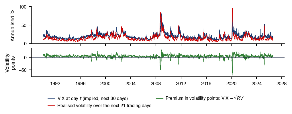
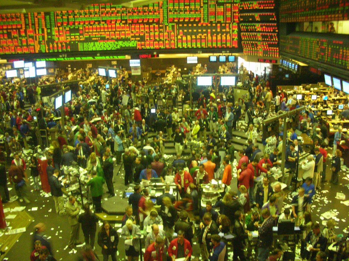



 MFM_ch12_greeks

 XFG (Quantlet prefix of Applied Quantitative Finance, Härdle, Chen & Overbeck) Advanced Methods in Quantitative Finance