Chapter 14: Deep Learning and Time-Series Foundation Models
Daniel Traian PELE
Bucharest University of Economic Studies IDA Institute Digital Assets Blockchain Research Center AI4EFin Artificial Intelligence for Energy Finance Romanian Academy, Institute for Economic Forecasting MSCA Digital Finance
Do Deep Networks Forecast Better than Classical Models?
“Deep learning allows computational models that are composed of multiple processing layers to learn representations of data with multiple levels of abstraction.” — LeCun, Bengio & Hinton (2015)
The signal is in the volatility, not in the mean (S&P 500 since 2000, 6 718 days)
Lag-1 autocorrelation: \(-\)0.099 for returns, 0.29 for absolute returns
Returns: no model beats the zero forecast on the S&P 500 and Bitcoin
After the correction for multiple testing
Volatility (SPY, 979 days): mean QLIKE (quasi-likelihood) loss 0.223 for zero-shot Chronos-2 and 0.226 for log-HAR
The difference is not significant (Diebold–Mariano test, \(p\) = 0.539)
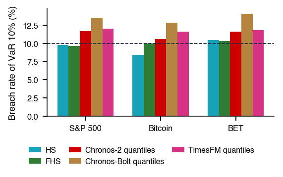
Left tail: raw Chronos-2 breaches its VaR (Value-at-Risk) 1% on 1.67% of S&P 500 days
On the S&P 500, filtered historical simulation (FHS) has the lowest loss for the (VaR, ES) pair
Deep learning allows computational models that are composed of multiple processing layers to learn representations of data with multiple levels of abstraction.
LeCun, Bengio & Hinton (2015) describe deep learning as learning representations of data through successive processing layers. The chapter asks whether such models forecast financial series better than the classical models of Chapters 5–9. It also tests time-series foundation models, available since 2024: networks pretrained on billions of observations from other series and used zero-shot, that is, with no estimation on the target series. Their pretraining corpora are dominated by non-financial series (energy, transport, weather, web).
A flexible model can only learn the signal that is in the data. In S&P 500 (Standard & Poor's) daily returns since 2000 (6,718 days), the lag-1 autocorrelation of returns is −0.099, and the 15 of 50 lags that fall outside the 95% band are small and of changing sign. The autocorrelation of absolute returns is 0.29 at lag 1 and 0.13 at lag 50, and all 50 lags fall outside the band. The signal is in the volatility, not in the mean.
The three tests follow this pattern. For returns, after the correction for multiple testing, no model beats the zero forecast on the S&P 500 and Bitcoin; on the S&P 500, TimesFM-2.5 is significantly worse than it (out-of-sample \(R^2\) −3.35%, Diebold–Mariano test, DM, \(p\) = 0.001). For the realised variance of SPY, over 979 test days, Chronos-2 has a mean QLIKE (Quasi-LIKElihood, loss function) loss of 0.223 and log-HAR 0.226, a difference that is not significant (DM \(p\) = 0.539). In the left tail, raw Chronos-2 has too many VaR (Value-at-Risk) 1% breaches on the S&P 500 (1.67% of days, Kupiec \(p\) = 0.001), and filtered historical simulation (FHS) has the lowest FZ0 (Fissler–Ziegel loss, zero-homogeneous version) loss. The chapter therefore shows how to evaluate a new model: against the right benchmark for each target, after the release of its weights, and with the inference that fits the type of comparison.
Mean QLIKE losses (lower is better) of the eight volatility models for the realised variance of SPY, one-day-ahead forecasts: left, the full test period (979 days); right, only the days after 3 November 2025 (218 days), when the weights of all three foundation models had been released. Interactive chart: “QLIKE Losses of Eight Volatility Models (1/3)” →
What you will be able to do
Derive vanishing gradients from the impulse responses of a vector autoregression (VAR) and the cell state of the LSTM (long short-term memory) as an AR(1) process.
Compute point, volatility and VaR/ES forecasts from a zero-shot quantile grid.
Interpret the comparison with the right benchmark for each target: the zero forecast for returns, log-HAR for volatility, FHS for the tails.
Interpret the tests of a new model: nesting, multiplicity, calibration, contamination and power.
Time-Series Foundation ModelsZero-shot forecasting, the three models tested, from a quantile grid to VaR and ES, contamination.
Test 1: Forecasting ReturnsOut-of-sample \(R^2\) against the zero forecast, nested models and multiple testing.
Test 2: Forecasting Realised VolatilityThe HAR (Heterogeneous AutoRegressive, model) model, the QLIKE loss, the DM, MCS (Model Confidence Set) and Giacomini–White tests.
Test 3: VaR 1% and ES 2.5%Breach rates, the COVID-19 crash, the PIT, comparing (VaR, ES) pairs and conformal recalibration.
The chapter asks whether deep neural networks, and the time-series foundation models built from them, forecast financial series better than the classical models of Chapters 5–9. The question is posed separately for three targets: the conditional mean of returns, the conditional variance and the lower tail of the conditional distribution. Each target has its own benchmark, chosen because it is hard to beat on that target, and each comparison uses the evaluation tools of Chapter 8: loss differentials, tests of equal predictive ability and backtests.
The section fixes the targets and their benchmarks and then shows, with the autocorrelation function of the S&P 500, where the predictable part of daily returns lies.
Can Deep Networks Forecast Better than the Classical Models?
Deep learning denotes models built from many layers of simple non-linear units whose parameters are estimated from data. Since 2024 a new class of such models has been available for time series: foundation models, networks pretrained once on billions of observations from other series and then applied to a new series with no estimation on it. Their pretraining corpora are dominated by non-financial series from energy, transport, weather and web traffic. Whether what they learn there transfers to financial returns is an empirical question, and the chapter answers it with the same tests that were applied to GARCH (Generalised AutoRegressive Conditional Heteroskedasticity), HAR and the risk models in earlier chapters.
The chapter has two parts:
Networks for sequences, attention and the foundation models, with Test 1 on returns.
Test 2 on realised volatility and Test 3 on left-tail risk, measured by value-at-risk (VaR) at the 1% level and expected shortfall (ES) at the 2.5% level, followed by two case studies and a section on artificial intelligence (AI) for scientific discovery.
The comparisons are designed so that a new model is not favoured by the design. Every model forecasts one day ahead, every forecast uses only information available at the forecast origin, and every comparison is made against the benchmark that is hardest to beat on the target in question.
In brief
Question: do deep networks forecast better than the classical models of Chapters 5–9?
Targets: returns, volatility and tail risk
Deep learning: models built from many layers of simple non-linear units, trained on data
Time-series foundation models (since 2024): networks pretrained on billions of observations from other series, used with no estimation on the target series
Why test them: their pretraining corpora are dominated by non-financial series (energy, transport, weather, web)
The daily log return in per cent, \(r_t = 100\ln(P_t/P_{t-1})\), where \(P_t\) is the closing price on day \(t\). Its conditional mean has a very low signal-to-noise ratio: predictable patterns attract traders, and trading removes them, as discussed under market efficiency in Chapter 2. The benchmark for the mean is therefore the zero forecast, which estimates nothing and cannot overfit.
The conditional variance. Volatility is persistent and clusters in time (Chapters 1 and 5), so there is a signal a flexible model can learn. The benchmark is log-HAR, the heterogeneous autoregressive model in logs: the logarithm of realised variance is regressed on its own daily, weekly and monthly averages. Its exact form is given in Test 2.
The shape of the lower tail. The value-at-risk at level 1%, VaR 1%, is the daily loss exceeded with probability 1%, and the expected shortfall at level 2.5%, ES 2.5%, is the average loss on the worst 2.5% of days (Chapter 7). The benchmark is filtered historical simulation (FHS): returns are standardised by a volatility from a GARCH model (generalised autoregressive conditional heteroskedasticity, Chapter 5), the empirical quantile of the standardised returns is taken, and it is multiplied by the forecast volatility.
In brief
Returns\(r_t = 100\ln(P_t/P_{t-1})\) (conditional mean), \(P_t\) the close on day \(t\)
Very low signal-to-noise ratio: predictable patterns are traded away (Chapter 2)
Benchmark: the zero forecast
Volatility (conditional variance): persistent and clustered (Chapters 1 and 5), a signal to learn
Benchmark: log-HAR, log realised variance regressed on its daily, weekly and monthly averages (heterogeneous autoregressive, Test 2)
Tail risk: the shape of the lower tail, not only the centre (Chapter 7)
VaR 1% (value-at-risk): the daily loss exceeded with probability 1%
ES 2.5% (expected shortfall): the average loss on the worst 2.5% of days
Benchmark: FHS (filtered historical simulation)
FHS: the empirical quantile of returns standardised by a GARCH volatility (generalised autoregressive conditional heteroskedasticity, Chapter 5), times the forecast volatility
Before any model is fitted, the autocorrelation function shows where a flexible model can find predictable structure. For a series of \(T\) observations that are independent and identically distributed (i.i.d.) with finite variance, the sample autocorrelation at any fixed lag is approximately Normal with mean zero and standard deviation \(1/\sqrt{T}\). The band \(\pm 1.96/\sqrt{T}\) is therefore a pointwise 95% range for each lag under that null; it is not a simultaneous band for all lags at once.
The autocorrelations of returns measure linear predictability of the mean. The autocorrelations of absolute returns \(|r_t|\) measure the persistence of the size of moves, that is, of volatility. For absolute returns the band is valid under the null that \(|r_t|\) is i.i.d. and \(E[r_t^2] < \infty\); when these conditions fail, a robust band is needed. The two functions answer different questions, and a weak signal in one says nothing about the other.
The interactive chart has the lag in trading days on the horizontal axis and the autocorrelation on the vertical axis, with the light-blue band marking \(\pm 1.96/\sqrt{T}\). The first slider sets the first year of the sample, the second the number of lags shown, and the selector switches the volatility series between absolute and squared returns. The ▶ button moves the start of the sample year by year.
Question for the room For the S&P 500 since 2000, which series shows stronger linear persistence over the first 50 lags: returns or their absolute values?
Answer
The absolute values. Their autocorrelation is 0.29 at lag 1 and 0.13 at lag 50, and all 50 values lie outside the ±0.024 band. Returns have a lag-1 autocorrelation of −0.099 and 15 lags outside the band, small and of changing sign. A negative sign does not imply stronger persistence, and forecasting the mean and forecasting volatility are distinct problems. The plot suggests volatility clustering; forecast usefulness is checked out-of-sample. The band is an approximate pointwise reference under an i.i.d. null, not a simultaneous band for all lags.
On S&P 500 daily returns since January 2000, 6,718 days, the band is \(\pm 0.024\). The lag-1 autocorrelation of returns is −0.099, and 15 of the first 50 lags fall outside the band; they are small and their sign changes from lag to lag. The autocorrelation of absolute returns is 0.29 at lag 1 and still 0.13 at lag 50, and all 50 lags lie outside the band.
The predictable structure of daily returns is therefore in the volatility, not in the mean. Flexible models can find the volatility signal; in the mean there is little to find. Whether either signal yields useful forecasts is decided out of sample, in Tests 1 and 2.
Light-blue band: \(\pm 1.96/\sqrt{T} = \pm\)0.024 (\(T\): number of days), the 95% range of an autocorrelation under i.i.d. returns (independent and identically distributed)
Returns: lag-1 autocorrelation \(-\)0.099
15 of 50 lags outside the band, small and of changing sign
Absolute returns: 0.29 at lag 1, 0.13 at lag 50
All 50 lags outside the band: persistent volatility clustering
The band assumes \(|r_t|\) i.i.d. with \(E[r_t^2] < \infty\); otherwise use a robust band
Flexible models can find the volatility signal, not much in the mean
The three targets differ in how much signal they contain, and each is compared with its own benchmark: the zero forecast for returns, log-HAR for realised variance and FHS for the tail. The autocorrelations already suggest the pattern of the results: little linear structure in the mean, strong and persistent structure in volatility.
Neural Networks for Sequences
This section builds the recurrent networks used in the chapter from the multilayer perceptron of Chapter 13. The central difficulty is memory: a network that processes a sequence step by step must carry information from distant days to today, and the gradient that trains it must travel back over the same distance. The section shows why the gradient of a simple recurrent network vanishes, by relating it to the impulse responses of a vector autoregression, and why the cell state of the LSTM behaves like an AR(1) process whose coefficient the network can set close to one.
From the Multilayer Perceptron to Deep Learning (1/3)
The multilayer perceptron (MLP) of Chapter 13 is the basic building block. Each layer applies a non-linear function to a linear combination of the output of the previous layer:
In (14.1),\(x\) is the input vector, \(h^{(\ell)}\) the output of layer \(\ell\), and \(W^{(\ell)}\) and \(b^{(\ell)}\) the weight matrix and bias vector of that layer, estimated from the data. The activation \(\varphi\) acts element by element. The usual choices are the rectified linear unit (ReLU) \(\max(0, z)\), the hyperbolic tangent \(\tanh\), and the sigmoid \(\sigma(z) = 1/(1+e^{-z})\), which maps the real line into \((0, 1)\) and is used later for the gates of the LSTM.
An MLP takes an input of fixed length. Applied to a time series, it sees a window of the last \(p\) observations and nothing before it, much like an autoregression of order \(p\). A network for sequences must instead carry information from one step to the next, so that the forecast at \(t\) can depend on the whole past. The question of the section is how a network can use information from distant days, and why the simplest recurrent network fails to do so.
In brief
Question of the section: how can a network use information from distant days?
Each layer applies a non-linear function to a linear combination of the previous layer
\(x\): input vector; \(h^{(\ell)}\): output of layer \(\ell\)
\(W^{(\ell)}\), \(b^{(\ell)}\): weight matrix and bias vector of layer \(\ell\), estimated from the data
\(\varphi\): activation, applied element by element: ReLU (rectified linear unit) \(\max(0, z)\), \(\tanh\), or the sigmoid \(\sigma(z) = 1/(1+e^{-z}) \in (0, 1)\)
An MLP takes a fixed window of inputs
A sequence network must carry information from one step to the next
From the Multilayer Perceptron to Deep Learning (2/3)
The parameters of a network are estimated by minimising a loss over the training sample. Backpropagation (Rumelhart, Hinton & Williams, 1986) computes the gradient of the loss with respect to every weight by the chain rule, layer by layer from the output back to the input. The weights are then updated with Adam, adaptive moment estimation (Kingma & Ba, 2015): a gradient step normalised by exponential averages of past gradients and of their squares, so that each weight has its own effective step size.
The loss determines which functional of the conditional distribution the network learns. For point forecasts the loss is the mean squared error (MSE), whose expectation is minimised by the conditional mean. For a quantile of level \(u\) the loss is the pinball loss:
where \(y\) is the realised value and \(q\) the quantile forecast. The loss (14.2) is asymmetric: an outcome above \(q\) costs \(u\) per unit of distance, an outcome below costs \(1-u\) per unit. Its expectation is minimised by the true \(u\)-quantile, which is why a network trained with (14.2) at several levels outputs a quantile grid. The foundation models of this chapter are trained in this way, and the same loss reappears as the scoring rule for VaR.
The universal approximation theorem of Hornik, Stinchcombe & White (1989) states that a network that is wide enough approximates any continuous function on a compact set arbitrarily well. The theorem is silent on the sample size needed to estimate such a network. With one financial series of a few thousand daily observations, sample size is the binding constraint, and the network must be regularised: by early stopping, by weight decay, a penalty on the size of the weights, and by averaging forecasts over several random initialisations (seeds). Because the data are a time series, the validation block used for early stopping must follow the training block in time.
The methods that made deep learning practical are surveyed by LeCun, Bengio & Hinton (2015); Hopfield and Hinton received the 2024 Nobel Prize in Physics. In finance the documented gains are cross-sectional. Gu, Kelly & Xiu (2020) find them on a cross-section of thousands of stocks, not on one index, and Fischer & Krauss (2018) apply LSTMs to the constituents of the S&P 500 to forecast which stocks beat the next-day cross-sectional median. This chapter forecasts single aggregate series: two indices and Bitcoin.
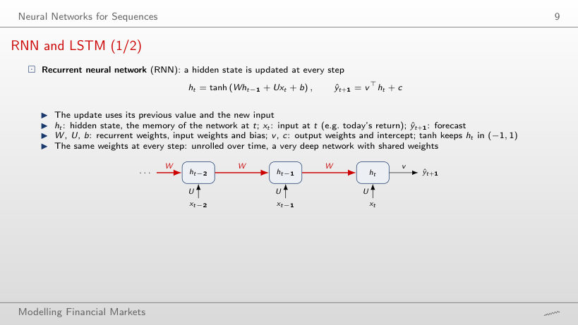
A recurrent neural network (RNN) keeps a hidden state \(h_t\), the memory of the network at time \(t\), and updates it at every step from its previous value and the new input:
In (14.3),\(x_t\) is the input at \(t\), for example today's return, \(W\) the matrix of recurrent weights, \(U\) the input weights and \(b\) a bias; \(v\) and \(c\) are the output weights and intercept that turn the state into the forecast \(\hat y_{t+1}\). The \(\tanh\) keeps every component of \(h_t\) in \((-1, 1)\).
The same weights are used at every step. Unrolled over time, as in the diagram, the RNN is a very deep network in which every layer shares the weights \(W\) and \(U\): the state \(k\) steps back reaches today's state through \(k\) applications of the same map. This depth is what allows the network to remember, and it is also the source of the training problem analysed two frames below.
The long short-term memory network (LSTM) of Hochreiter & Schmidhuber (1997) adds a second state, the cell state \(c_t\), and three gates that decide what to forget, what to write and what to show:
Here \(f_t\) is the forget gate, \(i_t\) the input gate and \(o_t\) the output gate; each has its own weights \(W_\bullet\),\(U_\bullet\),\(b_\bullet\) with \(\bullet \in \{f, i, o\}\). Note that in (14.4)\(W_\bullet\) weights the input and \(U_\bullet\) the previous state, the reverse of the letters in (14.3). Because the gates pass through the sigmoid, each component lies in \((0, 1)\): a gate near 0 blocks, a gate near 1 lets through. The vector \(g_t\) is the candidate new content, \(c_t\) the long-term memory, \(h_t\) the output, and \(\odot\) the element-by-element product.
The key line of (14.4) is the cell update \(c_t = f_t \odot c_{t-1} + i_t \odot g_t\). The old memory is carried forward multiplied only by the forget gate, not by a weight matrix followed by a squashing function. The gated recurrent unit (GRU) is a lighter variant with two gates that keeps this additive structure.
\(W_\bullet\) weights the input and \(U_\bullet\) the previous state here, reversing the RNN letters
\(f_t\): forget gate, \(i_t\): input gate, \(o_t\): output gate; each has its own weights \(W_\bullet\), \(U_\bullet\), \(b_\bullet\), \(\bullet \in \{f, i, o\}\)
\(\sigma\): sigmoid; a gate near 0 blocks, near 1 lets through
\(g_t\): candidate new content; \(c_t\): cell state, the long-term memory
Training an RNN requires the effect of old states on today's state. Backpropagation through time computes it by the chain rule, multiplying one Jacobian per step:
The matrix \(\partial h_T/\partial h_{T-k}\) gives the change in \(h_T\) per unit change in the state \(k\) steps earlier, and \(D_t\) is the diagonal matrix of the slopes \(\varphi'\) of the activation at step \(t\). By submultiplicativity of the spectral norm, \(\lVert AB\rVert_2 \le \lVert A\rVert_2\lVert B\rVert_2\), the product in (14.5) is bounded (Pascanu, Mikolov & Bengio, 2013):
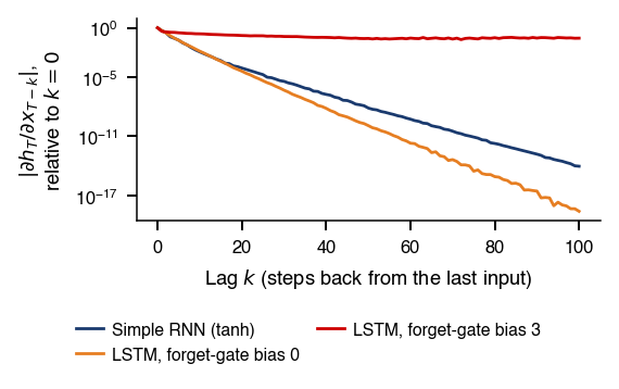
The spectral norm \(\lVert W\rVert_2\) is the largest factor by which \(W\) stretches a vector, and \(\gamma_\varphi\) is the largest slope of the activation, equal to 1 for \(\tanh\). If \(\gamma_\varphi \lVert W\rVert_2 < 1\), the bound (14.6) shrinks geometrically in \(k\): the gradient vanishes, and the network cannot learn dependence on distant steps. The scalar case makes the speed concrete (Bengio, Simard & Frasconi, 1994): with \(|w| = 0.9\) the gradient falls to 0.12 after 20 steps and to 0.005 after 50 steps.
The opposite case, a product that grows without bound, is the exploding gradient. It is handled by clipping the norm of the gradient before each update. Vanishing is the harder problem, and its remedy is architectural: gating, as in the LSTM.
In brief
Training needs the effect of old states on today's state
Backpropagation through time multiplies one Jacobian per step
The bound (14.6) has a familiar time-series interpretation. Let \(h^*\) be a fixed point of the network, a state that reproduces itself when the input is zero, and let \(D\) be the diagonal matrix of the activation slopes at \(h^*\). Linearising (14.3) around \(h^*\) gives
\[h_t - h^* \approx A\,(h_{t-1} - h^*) + D U x_t, \qquad A = D W.\]
(14.7)
Near its fixed point, the hidden state follows a first-order vector autoregression, VAR(1), with coefficient matrix \(A\) and input \(D U x_t\).
In this approximation \(\partial h_T/\partial h_{T-k} = A^k\), which is exactly the impulse response of the VAR at horizon \(k\), and the standard theory of stable VARs applies. Let \(\rho(A)\) be the spectral radius, the largest absolute eigenvalue of \(A\). If \(\rho(A) < 1\), the VAR is stable and \(\lVert A^k\rVert \to 0\) geometrically as \(k \to \infty\); if \(\rho(A) > 1\), the responses explode. At finite horizons \(\lVert A^k\rVert\) can grow transiently when \(A\) is not normal, that is, when \(AA^\top \ne A^\top A\).
A stable RNN near its fixed point is therefore a short-memory model, like any stationary VAR: the influence of a shock, and with it the gradient, decays geometrically. The derivation is exercise A4 of Seminar 14, and the relation between norms, spectral radius and explosion is detailed in the Appendix.
In brief
Linearise around a fixed point \(h^*\) of the network
\[
h_t - h^* \approx A\,(h_{t-1} - h^*) + D U x_t, \qquad A = D W
\]
Fixed point: a state that reproduces itself when the input is zero
\(D\): the slopes of the activation at \(h^*\)
The hidden state follows a VAR(1) (vector autoregression) with coefficient matrix \(A\)
\(\partial h_T / \partial h_{T-k} = A^k\) is the impulse response of this VAR at horizon \(k\)
\(\rho(A)\): spectral radius, the largest absolute eigenvalue of \(A\)
\(\rho(A) < 1\): stable VAR, \(\lVert A^k\rVert \to 0\) geometrically as \(k \to \infty\)
At finite horizons \(\lVert A^k\rVert\) can grow transiently if \(A\) is not normal (\(A A^\top \ne A^\top A\))
\(\rho(A) > 1\): they explode
A stable RNN near its fixed point is a short-memory model, like any stationary VAR
Along the cell state of (14.4) the only multiplier is the forget gate. On the direct path, \(\partial c_T/\partial c_{T-k} = \prod_{j=0}^{k-1} f_{T-j}\), with no weight matrix and no activation slope in the product. The cell update \(c_t = f_t \odot c_{t-1} + i_t \odot g_t\) is an autoregression of order one with a random coefficient \(f_t\).
A simplified scalar cell with a constant forget gate \(f\) makes the point exact. When the gate inputs are zero, \(f = \sigma(b_f)\), where \(b_f\) is the bias of the gate, and the cell is an AR(1) with coefficient \(f\). With a white-noise input \(i_t g_t\) and a stationary start,
where \(k_{1/2}\) is the half-life, the lag at which half of the memory is left. With \(b_f = 0\), the gate is \(f = 0.5\) and after 50 steps \(0.5^{50} \approx 9 \times 10^{-16}\) of the memory remains. With \(b_f = 3\),\(f = 0.953\), the memory left after 50 steps is \(0.953^{50} \approx 0.09\), and the half-life is 14 steps. Setting the forget-gate bias high is what lets the LSTM remember.
The decay in (14.8) is still geometric. Long memory decays hyperbolically: \(\rho_k \sim C k^{2d-1}\), where \(\rho_k\) is the autocorrelation at lag \(k\),\(d \in (0, \tfrac12)\) the memory parameter and \(C > 0\) a constant. On S&P 500 absolute returns, the fitted geometric decay gives \(\rho_{150} = 0.027\), against 0.059 observed (Appendix). A single LSTM cell can be persistent but not long-memory; the HAR model of Test 2 approximates long memory with three averages instead.
In brief
Along the cell state the only multiplier is the forget gate
\(\partial c_T / \partial c_{T-k} = \prod_{j=0}^{k-1} f_{T-j}\) on the direct path
\(c_t = f_t \odot c_{t-1} + i_t \odot g_t\): an AR(1) with a random coefficient
Simplified scalar cell with a constant forget gate \(f\): an AR(1) with coefficient \(f\)
\(f = \sigma(b_f)\) when the gate inputs are zero; \(b_f\): its bias
With a white-noise input \(i_t g_t\) and a stationary start, \(\operatorname{Corr}(c_t, c_{t-k}) = f^k\) decays geometrically
With \(b_f = 0\), the forget gate is \(f = 0.5\), and after 50 steps \(0.5^{50} \approx 9 \times 10^{-16}\) of the memory is left
\(b_f = 3\): \(f = 0.953\), and \(0.953^{50} \approx 0.09\) of the memory is left after 50 steps
Half-life 14 steps (the \(k\) with \(f^k = \frac12\), \(k = \ln 0.5/\ln f\))
Long memory decays hyperbolically: \(\rho_k \sim C k^{2d-1}\)
With \(\rho_k\) the autocorrelation at lag \(k\)
\(d \in (0, \frac12)\) the memory parameter, \(C > 0\) a constant
S&P 500 absolute returns: the fitted geometric decay gives \(\rho_{150}\) = 0.027, against 0.059 observed (Appendix)
A simple RNN near its fixed point is a stable VAR(1), and its gradient decays like the impulse responses of that VAR. The LSTM escapes the decay along its cell state, which is an AR(1) whose coefficient the forget gate can set near one, but the decay remains geometric. The next section removes the recurrence altogether.
Attention and Transformers
Attention links any two time steps directly, without the product of Jacobians that makes the gradient of an RNN vanish. The price is a cost that grows with the square of the number of inputs. The section defines attention, shows how patching reduces its cost, and explains how positions are added to a mechanism that by itself ignores order. These are the components of the foundation models tested in the rest of the chapter.
The question of the section is how a network can link today directly to a day 500 days back. Attention (Vaswani et al., 2017) answers it without recurrence. Each time step forms a query and compares it with the key of every step it is allowed to see; the answer is a weighted average of the values of those steps, with weights that grow with the similarity of query and key:
\[\operatorname{Attention}(Q, K, V) = \operatorname{softmax}\!\left(\frac{Q K^\top}{\sqrt{d_k}}\right) V, \qquad Q = XW_Q,\; K = XW_K,\; V = XW_V.\]
(14.9)
In (14.9),\(X\) holds the inputs, one row per time step, and \(W_Q\),\(W_K\),\(W_V\) are learned weight matrices that produce the queries \(Q\), the keys \(K\) and the values \(V\). The three matrices are different projections of the same inputs, so a step can look for one kind of pattern (its query) while being found by others through a different one (its key).
In brief
Question of the section: how can a network link today directly to a day 500 days back?
Without the product of Jacobians that makes the RNN gradient vanish
Each time step asks a question (query) and compares it with the key of every step it is allowed to see
\[
\operatorname{Attention}(Q, K, V) = \operatorname{softmax}\!\left(\frac{Q K^\top}{\sqrt{d_k}}\right) V, \qquad Q = XW_Q,\; K = XW_K,\; V = XW_V
\]
The matrix \(QK^\top\) contains the similarity score of every pair of steps. The scores are divided by \(\sqrt{d_k}\), where \(d_k\) is the length of a key vector: the variance of a dot product grows with \(d_k\), and without the scaling the softmax would saturate, giving almost all weight to one step and almost zero gradient to the others. The softmax then turns each row of scores \(s_1, \dots, s_n\) into positive weights that sum to one:
Two properties follow. There is no product of Jacobians over time: any past step is one hop away from today, so the gradient path does not lengthen with the lag. And the cost is \(O(n^2)\): the number of scores, and the work, grow with the square of the number of inputs \(n\). A worked example with three steps and a causal mask, which forbids a step from attending to the future, is in Further Topics.
In brief
\(QK^\top\): the similarity score of every pair of steps
\(d_k\): length of a key vector
Dividing by \(\sqrt{d_k}\) keeps the scores from saturating the softmax
softmax turns each row of scores \(s_1, \dots, s_n\) into positive weights that sum to one
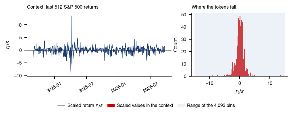
The quadratic cost of (14.9) makes one token per day expensive for long contexts. Patching groups consecutive observations into one token, so the number of tokens, and with it the number of attention scores, falls. The chart shows how the two foundation models of the chapter that use patches read the same context of S&P 500 daily returns.
The interactive chart has two panels with the day relative to the forecast origin on the horizontal axis and the daily return in per cent on the vertical axis; each shaded block is one patch and becomes one token. The first slider sets the patch length of the top panel (2 to 64 days), the second the context length (128 to 512 days); the bottom panel keeps the 32-day patches of TimesFM-2.5. The ▶ button runs through the patch lengths.
Question for the room In the illustration, 512 days form 16-day patches. How many entries are in one attention head’s matrix, assuming full attention only among context tokens?
Answer
There are 512/16 = 32 tokens and 32² = 1,024 ordered pairs, against 512² = 262,144 if each day were a token: 16² = 256 times fewer. TimesFM-2.5 uses patches of 32 days: 16 tokens and 256 entries. This is the simplified calculation for one head, without additional tokens; a multi-head layer has one such matrix per head.
With a 512-day context and 16-day patches, as in Chronos-2, there are 512/16 = 32 tokens and \(32^2 = 1{,}024\) ordered pairs in the attention matrix of one head, against \(512^2 = 262{,}144\) if every day were a token: \(16^2 = 256\) times fewer. TimesFM-2.5 uses 32-day patches: 16 tokens and 256 entries. The count is for one head with attention among context tokens only; a multi-head layer has one such matrix per head.
Attention treats its inputs as a set: permuting the rows of \(X\) permutes the output in the same way, so the order of the days is lost. A positional encoding adds it back. The original Transformer adds sinusoids of the position to the inputs; Chronos-2 uses rotary embeddings (RoPE), which rotate each query and key by an angle proportional to its position. With rotations, the score of two steps depends on how far apart they are, not on where they sit in the context, which suits a series whose dynamics do not depend on calendar position.
Patching (Nie et al., 2023) makes a token out of a block of consecutive observations. A learned map turns each block into a vector of fixed length, the embedding. With 512 daily returns in patches of 16 days, attention works on 32 tokens and computes \(32^2\) instead of \(512^2\) scores, 256 times fewer. The chart on the previous frame shows the last 512 daily returns of the S&P 500 split as Chronos-2 (16 days) and TimesFM-2.5 (32 days) read them.
Global models, trained across many series rather than on one, preceded the foundation models: DeepAR (Salinas et al., 2020), N-BEATS (Oreshkin et al., 2020) and PatchTST (Nie et al., 2023). Foundation models push the same idea to very large and diverse corpora.
In brief
Positional encoding: attention treats its inputs as a set, so order is added
Sinusoids in the original Transformer; rotary embeddings in Chronos-2
Rotary embeddings (RoPE): each query and key is rotated by an angle proportional to its position
So the score of two steps depends on how far apart they are, not on where they sit in the context
Patching (Nie et al. (2023)): a token is a block of consecutive observations
A learned map turns it into a vector of fixed length (embedding)
512 daily returns in patches of 16 days: 32 tokens, 256 times fewer attention scores (\(32^2\) instead of \(512^2\))
Chart: the last 512 daily returns of the S&P 500
Split as Chronos-2 (16 days) and TimesFM-2.5 (32 days) read them
Attention removes the long gradient path of the RNN at a quadratic cost, patching reduces that cost by grouping days into tokens, and positional encodings restore the order that attention ignores. The next section assembles these components into pretrained models and specifies what they receive and what they return.
Time-Series Foundation Models
A foundation model is estimated once, on a corpus of many series, and then used without further estimation on series it was not trained on. The section defines zero-shot forecasting, describes the three models tested in the chapter and shows how their output, a grid of quantiles, yields point forecasts, volatility forecasts, VaR and ES. It closes with the specific risk of these models: that the test period was already seen in pretraining.
The question of the section is whether a model pretrained on other series can forecast a financial series it never saw in training. A foundation model is a large network pretrained once on a very broad corpus and then used on new tasks. The idea comes from large language models (LLMs), which are pretrained on text and then applied to tasks they were not specifically trained for. For finance the appeal is practical: one model for thousands of series, with no estimation for each series.
Three families of time-series foundation models are discussed. Chronos (Ansari et al., 2024) turns values into the tokens of a language model. TimesFM (Das et al., 2024) is a decoder-only Transformer that reads the series in patches. Moirai (Woo et al., 2024) accepts any number of variables and outputs a mixture distribution (Appendix); it is not tested in the chapter because of its non-commercial licence.
In brief
Question of the section: can a model pretrained on other series forecast a financial series it never saw in training?
Foundation model: a large network pretrained once on a very broad corpus, then used on new tasks
An idea borrowed from large language models (LLM)
Appeal for finance: one model for thousands of series, no estimation per series
In zero-shot forecasting the parameters \(\hat\theta\) of the network are fixed in pretraining and are not re-estimated on the target series. At time \(T\) the model receives only the recent history of the series, the context, and returns a grid of quantiles for each horizon:
In (14.11),\(F_{\hat\theta}\) is the pretrained network, the same for every series; \(C\) is the context length, 512 days in this chapter; \(H\) is the forecast horizon; and \(\hat q_{u_k, T+h}\) is the forecast \(u_k\)-quantile of the value at \(T+h\). The output is a distribution described by \(K\) quantiles, not only a point.
Fine-tuning, further training on the target series, is possible but is not used. The chapter tests the promise of no estimation itself. The specific risk of the approach is that the target series, or the test period, may be part of the pretraining corpus; this is the subject of the frame on leakage.
In brief
Zero-shot forecasting: the parameters \(\hat\theta\) are fixed in pretraining
Ansari et al. (2024) turn the values of a series into tokens and train a language model, T5 (Text-to-Text Transfer Transformer), with the cross-entropy loss. Keeping tokens means the language-model architecture stays unchanged. A distribution over tokens imposes no parametric shape on the forecast: it can be skewed or multimodal.
The values are first scaled by the mean absolute value of the context and then quantised to the nearest of a fixed set of bin centres:
In (14.12),\(s\) is the mean absolute value of the \(C\) values in the context, the \(c_j\),\(j = 1, \dots, 4{,}093\), are equally spaced bin centres in \([-15, 15]\),\(30/4{,}092 = 0.0073\) apart, to which special tokens are added, and \(z_t\) is the token of \(x_t\), the index of the nearest centre. To forecast, the model samples future tokens \(z\), maps them back to values \(s\,c_z\) and reads the quantiles from the samples. What the scaling and the bins do to daily returns is shown in Further Topics.
The pretraining corpus consists of public datasets from energy, transport, retail, weather, web, finance and economics. It is augmented with two kinds of synthetic series: TSMixup series, random convex combinations of real series, and KernelSynth series, paths of Gaussian processes with randomly combined covariance kernels. The original Chronos models, based on T5, have 8 to 710 million parameters; Chronos-Bolt, tested here, has 9 to 205 million.
In brief
Ansari et al. (2024): turn values into tokens and train a language model with cross-entropy
The language model: T5, Text-to-Text Transfer Transformer
Why tokens: the language-model architecture stays unchanged
A distribution over tokens imposes no parametric shape (it can be skewed or multimodal)
The chapter tests three models, all run on a CPU (central processing unit) with a 512-day context. Chronos-Bolt replaces token sampling with patches and a direct quantile output; the small version used here has 48 million parameters, 16-day patches, quantiles from 10% to 90%, and its weights were released on 25 November 2024. Chronos-2 (Ansari et al., 2025) uses robust scaling and attention both across time and across groups of related series; it has 119 million parameters, 16-day patches, and 21 quantile levels from 1% to 99% (1%, 5%, 10%, …, 95%, 99%); its weights were released on 30 October 2025.
TimesFM (Das et al., 2024) was pretrained on about \(10^{11}\) time points. Version 2.5, released as timesfm-2.5-200m, has 231 million parameters when counted on the loaded model, uses 32-day patches, outputs a mean and the quantiles from 10% to 90%, and its weights were released on 1 October 2025. Parameter counts in the table are those of the loaded models.
The release dates of the weights matter for the evaluation: they bound what the models could have seen. Days after the last release are free of one form of contamination, which the frame on leakage uses to define a post-release window. Other foundation models and their corpora are listed in the Appendix.
In brief
Model
Parameters
Patch
Quantile levels
Weights released
Chronos-Bolt (small)
48 M
16
10%–90%
25.11.2024
TimesFM-2.5
231 M
32
mean, 10%–90%
01.10.2025
Chronos-2
119 M
16
21: 1%, 5%, 10%, …, 95%, 99%
30.10.2025
Chronos-Bolt: patches and a direct quantile output instead of token sampling
Chronos-2 (Ansari et al. (2025)): robust scaling, attention across time and across groups of related series
TimesFM (Das et al. (2024)): pretrained on about \(10^{11}\) time points
Parameters are counted on the loaded models
TimesFM-2.5 is released as timesfm-2.5-200m
All run on a CPU (Central Processing Unit) with a 512-day context
The release dates of the weights bound what the models could have seen
The model returns quantiles \(q_u\) at levels \(u_1 < \dots < u_K\), with \(P(Y \le q_u) = u\), where \(Y\) is the future value and \(K\) the number of levels. A grid is useful because the same quantiles give the point forecast, the volatility forecast and the tail risk, so one model serves all three tests of the chapter.
Two point forecasts can be read from the grid: the median \(q_{0.5}\), and the mean \(\int_0^1 q_u\,du\), the average of all quantiles. More generally, for any function \(g\) for which the mean exists,
\[E[g(Y)] = \int_0^1 g(q_u)\,du,\]
(14.13)
because \(Y\) has the same distribution as \(q_U\) with \(U\) uniform on \((0,1)\). This is the formula used when \(Y\) is a log variance and the target is the variance itself, with \(g = \exp\). If \(g\) is increasing, \(g(q_u)\) is also the \(u\)-quantile of \(g(Y)\); formula (14.13) does not need this property.
A check shows the difference. Let \(Y\) be uniform on \((-1, 1)\), so \(q_u = 2u - 1\), and \(g(y) = y^2\). Then \(\int_0^1 (2u-1)^2\,du = 1/3 = E[Y^2]\), although \((2u-1)^2\) is not a quantile function of \(Y^2\): it falls and then rises in \(u\).
In brief
The model returns quantiles \(q_u\) at levels \(u_1 < \dots < u_K\): \(P(Y \le q_u) = u\)
\(Y\): the future value; \(K\): the number of levels
Why a grid: the same quantiles give the point forecast, the volatility and the tail risk
So one model serves all three tests
Point forecasts from the grid
the median \(q_{0.5}\), or the mean \(\int_0^1 q_u\,du\), the average of all quantiles
for any function \(g\) with a finite mean: \(E[g(Y)] = \int_0^1 g(q_u)\,du\), because \(Y\) has the same distribution as \(q_U\) with \(U\) uniform (e.g. \(g = \exp\) when \(Y\) is a log variance)
If \(g\) is increasing, \(g(q_u)\) is also the \(u\)-quantile of \(g(Y)\)
Check: \(Y\) uniform on \((-1, 1)\), \(q_u = 2u - 1\), \(g(y) = y^2\): \(\int_0^1 (2u-1)^2\,du = 1/3 = E[Y^2]\), although \((2u-1)^2\) is not a quantile of \(Y^2\) (it falls, then rises in \(u\))
Below the lowest level of the grid, the model gives no information, and the rule chosen there changes the result. Holding \(q_u\) constant at \(q_{0.01}\) below 1% understates ES, because the true quantiles there are lower; extrapolating can err in either direction (exercises A1 and A7 of Seminar 14).
The problem is acute for the two models whose grid stops at 10%. For Chronos-Bolt and TimesFM, a request for VaR 1% returns the 10% quantile. The chapter's rule is linear interpolation between the levels of the grid, with \(q_u\) held flat below the lowest level. A worked example is in Further Topics.
In brief
Tail risk at level \(\alpha\) (Chapter 7), for a return \(Y\)
A test is out of sample only if the test period was never seen during training. For a foundation model it can be seen in four ways:
(i) the same series is in the pretraining corpus;
(ii) correlated series in the corpus carry the same shocks;
(iii) the developers select model versions on public benchmarks that overlap with the test;
(iv) the researcher's own look-ahead, when scalings, windows, seeds or contexts are chosen with test data.
The Chronos corpus includes financial series, for example daily exchange rates from 1990 to 2016, so it cannot be ruled out that the series of this chapter were seen in pretraining. The remedy for (i)–(iii) is a post-release window starting on 3 November 2025, a common cutoff after all three sets of weights were published. The window is short: about 220 trading days, or 320 calendar days for Bitcoin, which trades every day. Tests on it have low power, especially for VaR 1%. The window is free of weight contamination only if the checkpoint used predates it; for this reason the revision and the hash of the weights are pinned in the code (appendix on the corpora).
Channel (iv) is under the researcher's control: every scaling, window and estimate in the chapter uses only past data. Choosing the context length or the hyperparameters with hindsight remains possible even after the release, so a formal protocol is needed; it is given in the Appendix.
In brief
A test is out of sample only if the test period was never seen during training
It can be “seen” in four ways
(i) the same series is in the pretraining corpus
(ii) correlated series carry the same shocks
(iii) developers select model versions on overlapping public benchmarks
(iv) our own look-ahead: scalings, windows, seeds or contexts chosen with test data
The Chronos corpus includes financial series (e.g. daily exchange rates 1990–2016)
So we cannot rule out that our series were seen in pretraining
Remedy for (i)–(iii): a post-release window from 3 November 2025
A common cutoff after all three sets of weights were published
Short: about 220 trading days (320 calendar days for Bitcoin), hence low power, especially for VaR 1%
Free of weight contamination only if the checkpoint used predates the window: its revision and weight hash are pinned in the code (appendix on the corpora)
(iv) is under our control: every scaling, window and estimate uses only past data
Choosing the context or the hyperparameters with hindsight remains possible after the release
A zero-shot foundation model is a fixed map from a context window to a quantile grid. From the grid follow the mean, the median, the volatility and the pair (VaR, ES), but the lower tail beyond the last quantile is a modelling choice. Because the corpora may contain the test series, the results are also reported on the window after 3 November 2025.
Test 1: Forecasting Returns
The first test asks the oldest question in empirical finance with the newest models: does any model forecast tomorrow's return better than the zero forecast? The section describes the design, the out-of-sample \(R^2\) and the Diebold–Mariano test, and then the two corrections that a comparison of many models against a simple benchmark requires: the Clark–West adjustment for nested models and the adjustments for multiple testing.
The test uses daily returns of three markets. The S&P 500 and the BET, the index of the Bucharest Stock Exchange, start on 4 January 2016; Bitcoin starts on 1 January 2019. The test samples have 2,693 days for the S&P 500, 2,675 days for the BET and 2,818 days for Bitcoin, about ten years for the two indices and eight for Bitcoin, and they include the crash of March 2020 and the year 2022.
The three markets are chosen for their differences:
The S&P 500 is the most liquid equity market, where a simple signal would already have been traded away.
The BET is a smaller and less liquid market, where stale prices can create predictability.
Bitcoin trades around the clock, and its daily standard deviation is almost three times larger: 3.21% against 1.13% for the S&P 500.
Six models are compared with the zero forecast:
the historical mean;
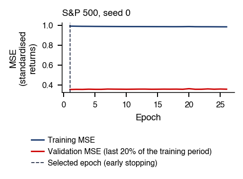
an AR(1), \(\hat r_t = \hat a + \hat b\, r_{t-1}\), estimated by least squares on the last 1,000 days and re-estimated daily;
an LSTM;
the three foundation models.
For the foundation models the point forecast is the median of the grid, which extreme values do not move; forecasts from the grid means are reported separately. Every forecast uses only data up to the previous close.
In brief
Question: does any model forecast tomorrow's daily return better than the zero forecast?
Test period: S&P 500 and BET from 04.01.2016, Bitcoin from 01.01.2019, to 18.09.2026
BET: Bucharest Stock Exchange index; 2 693 days (S&P 500), 2 675 (BET) and 2 818 (Bitcoin)
About ten years (eight for Bitcoin), including the March 2020 crash and 2022
Estimation also uses earlier data: the series start in 1990 (S&P 500), 1997 (BET) and 2014 (Bitcoin)
Why three markets
S&P 500: the most liquid equity market, where a simple signal would already be traded away
BET: a smaller, less liquid market, where stale prices can create predictability
Bitcoin: traded around the clock, with a daily standard deviation almost three times larger (3.21% against 1.13% for the S&P 500)
Models: historical mean, AR(1), LSTM, Chronos-2, Chronos-Bolt and TimesFM-2.5
AR(1): \(\hat r_t = \hat a + \hat b\, r_{t-1}\), least squares on the last 1,000 days, re-estimated daily
Foundation models: the grid median, a point forecast that extreme values do not move
Grid means are reported separately
Every forecast uses only data up to the previous close
where \(r_t\) is the realised return and \(\hat r_t\) the forecast made with data up to \(t-1\). A positive value in (14.15) means that the model has smaller squared errors than the zero forecast; unlike the in-sample \(R^2\), it can be negative, and is whenever the model does worse than zero.
Zero is preferred to the historical mean as the benchmark because the estimated mean adds estimation noise to the forecast. The literature uses both: zero is the benchmark of Gu, Kelly & Xiu (2020), the historical mean that of Campbell & Thompson (2008). With zero as the benchmark, the historical mean itself becomes one of the competing models.
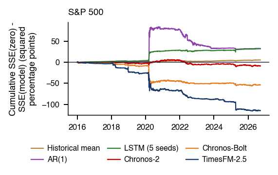
Using the mean of the grid, \(\int_0^1 q_u\,du\), instead of its median makes the foundation models worse. On the S&P 500, the out-of-sample \(R^2\) of the grid mean is −0.77% for Chronos-2 and −3.42% for TimesFM-2.5. The mean is pulled by the extreme quantiles, and in the mean of daily returns there is little signal to compensate for the added variance.
The uncertainty of \(R^2_{\text{OOS}}\) is measured with a block-bootstrap confidence interval (CI). A test period of the same length is rebuilt from blocks of 20 consecutive days drawn with replacement, 1,000 times, and the 2.5% and 97.5% percentiles of the resulting \(R^2\) values form the interval. Blocks rather than single days are drawn so that volatility clusters stay together.
The test of equal accuracy is the Diebold–Mariano (DM) test (Diebold & Mariano, 1995) on squared errors:
In (14.16),\(\bar d\) is the mean of the loss differential \(d_t\) over the \(n\) forecasts, and \(\hat V_{NW}\) is the long-run variance of \(d_t\), estimated by the Newey–West estimator, which is consistent under heteroskedasticity and autocorrelation (HAC). A positive DM means that the model has larger errors than the zero forecast. Under \(H_0\colon E[d_t] = 0\), DM is approximately standard Normal.
The approximation needs a finite, non-zero long-run variance of \(d_t\) and weak dependence. Here \(d_t = \hat r_t^2 - 2 r_t \hat r_t\), so what matters are the moments of \(r_t \hat r_t\), not necessarily the fourth moment of returns, \(E[r_t^4]\), which may not exist for heavy-tailed daily returns. How the LSTM of the test is trained is shown in Further Topics.
In brief
Block-bootstrap confidence interval (CI) for \(R^2\)
Rebuild a test period of the same length from blocks of 20 consecutive days drawn with replacement, 1,000 times
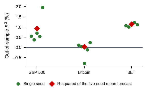
The chart summarises Test 1 for the three markets. It compares each model with the zero forecast through \(R^2_{\text{OOS}}\) of (14.15) and shows the uncertainty of each estimate through its 95% block-bootstrap interval. The full table, with the DM \(p\)-values, is in the Appendix.
The interactive chart groups the bars by market on the horizontal axis; the vertical axis is \(R^2_{\text{OOS}}\) against the zero forecast, in per cent, and each bar carries its 95% circular block-bootstrap interval with 20-observation blocks. Hovering over a bar shows the interval and the DM \(p\)-value. The slider moves the start of the evaluation from 2016 to the post-release window of 3 November 2025, and the ▶ button runs through the start years.
Question for the room Over the full S&P 500 test period, does the two-sided DM test at 5% establish that AR(1) or the LSTM outperforms the zero forecast?
Answer
No. AR(1) and the LSTM reduce the observed mean squared error by 0.94% and 0.93% (out-of-sample R²), but their two-sided DM p-values are 0.639 and 0.090. The test establishes neither superiority at 5% nor equality. TimesFM-2.5 is significantly worse than zero (R² −3.35%, DM p = 0.001). Only on the BET does the LSTM pass at 5% (R² +1.15%, p = 0.014), before the correction for multiple tests.
On the S&P 500 and Bitcoin, no model beats zero in the two-sided DM test. On the S&P 500, the AR(1) and the LSTM reduce the mean squared error by 0.94% and 0.93% relative to zero, but their two-sided DM \(p\)-values are 0.639 and 0.090; the test establishes neither superiority at 5% nor equality. The historical mean passes the Clark–West test for nested models (\(p\) = 0.007), but not the joint SPA (Superior Predictive Ability, test) test (\(p\) = 0.130); both tests are explained in the next frames.
TimesFM-2.5 is significantly worse than zero on the S&P 500: \(R^2_{\text{OOS}}\) is −3.35%, with DM \(p\) = 0.001. The standard deviation of its forecasts is 0.141%, three times that of the LSTM, and the extra variation of its forecasts adds to its squared errors.
On the BET, the LSTM has \(R^2_{\text{OOS}}\) = +1.15%, with a two-sided DM \(p\) of 0.014 and a one-sided \(p\) of 0.007. This is a small signal, and the following frames test it for nesting, for multiplicity and, in Further Topics, for stale prices.
In brief
\(R^2\) against the zero forecast (%), 95% block-bootstrap CIs
The zero forecast is nested in the historical mean and in the AR(1): each becomes the zero forecast when its coefficients are zero. Under the null that the larger model has no information, it only adds estimation noise to its forecasts, which raises its squared errors. The DM test then rejects too rarely, because the population differential is zero while the sample differential is biased against the larger model.
Clark & West (2007) add back the noise term and test the mean of the adjusted differential with a one-sided HAC \(t\)-test:
In (14.17),\(\hat r_{0,t}\) is the zero forecast of the small model, \(\hat r_{1,t}\) the forecast of the large model, and \(e_{0,t}\),\(e_{1,t}\) their errors \(r_t - \hat r_{\cdot,t}\). The term \((\hat r_{0,t} - \hat r_{1,t})^2\) is the cost of estimating coefficients that are zero under \(H_0\). The null is \(E[\tilde d_t] = 0\), and a large positive \(t\) means the large model adds information. Against the zero forecast, \(\tilde d_t = 2 r_t \hat r_t\); both tests need a finite, non-zero long-run variance of their differential.
The correction changes the conclusions. For the historical mean, the one-sided \(p\)-value falls from 0.048 (DM) to 0.007 (Clark–West) on the S&P 500, and from 0.041 to 0.003 on the BET. For the AR(1) on the S&P 500 it falls from 0.320 to 0.055. With the correction, the historical mean is significant in both markets, but the gain stays small: \(R^2_{\text{OOS}}\) of 0.15% on the S&P 500 and 0.30% on the BET. The BET AR(1) and rolling windows are in the Appendix.
In brief
The problem: zero is nested in the historical mean and AR(1)
Under \(H_0\) the larger model only adds estimation noise, so DM rejects too rarely
Clark–West (Clark & West (2007)): add back the noise term and test its mean, one-sided HAC \(t\)-test
\(\hat r_{0,t}\): zero forecast (small model); \(\hat r_{1,t}\): forecast of the large model; \(e_{0,t}\), \(e_{1,t}\): their errors \(r_t - \hat r_{\cdot,t}\)
\((\hat r_{0,t} - \hat r_{1,t})^2\): the cost of estimating coefficients that are zero under \(H_0\)
\(H_0\): \(E[\tilde d_t] = 0\); a large positive \(t\): the large model adds information
One-sided \(p\)-values, DM against Clark–West
both tests need a finite, non-zero long-run variance of the differential (for CW against the zero forecast, \(\tilde d_t = 2 r_t \hat r_t\))
Test 1 runs 6 models on 3 markets, 18 tests in all, and the smallest one-sided DM \(p\)-value is that of the BET LSTM, 0.007. A small \(p\)-value among many is weaker evidence than a single small \(p\)-value. If no model had a signal and the 18 tests were independent, at least one \(p < 0.05\) would appear with probability \(1 - 0.95^{18} = 0.60\).
The Bonferroni correction controls the probability of any false rejection, the family-wise error rate, by rejecting only when \(p < 0.05/M\) for \(M\) tests; here the threshold is \(0.05/18 = 0.0028\). The Holm procedure applies the same idea step by step: the smallest \(p\)-value is compared with \(0.05/M\), the next with \(0.05/(M-1)\), and so on, stopping at the first non-rejection. It controls the same error rate and rejects at least as often as Bonferroni.
Over the 18 tests, the Holm-adjusted \(p\)-value of the BET LSTM is 0.130. It is not significant: the signal on the BET does not survive when all the comparisons that were run are taken into account.
In brief
6 models \(\times\) 3 markets = 18 tests
The smallest one-sided DM \(p\) is the BET LSTM, 0.007
The problem: at least one \(p < 0.05\) would appear with probability \(1 - 0.95^{18} = 0.60\)
If no model had a signal and the tests were independent
Bonferroni: with \(M\) tests, reject only if \(p < 0.05/M\) (here 0.0028)
Holm: the same idea, applied step by step from the smallest \(p\)
Both control the probability of any false rejection
Holm-adjusted \(p\) over the 18 tests: 0.130, not significant
Bonferroni and Holm ignore the correlation between the tests, and the forecasts of six models on the same market are strongly correlated. Two bootstrap procedures use it. The step-down method of Romano & Wolf (2005) gives the BET LSTM an adjusted \(p\)-value of 0.016 within the six BET models. The test of superior predictive ability (SPA) of Hansen (2005) has the null that no model beats zero; its \(p\)-values are 0.018 on the BET, 0.130 on the S&P 500 and 0.354 on Bitcoin. Both procedures need finite, non-zero long-run variances of the differentials and a valid stationary bootstrap.
The conclusion depends on the family of tests fixed in advance. The statement "some model beats zero on the BET" holds if the BET was chosen in advance as the test family. If the three markets form the family, the Holm correction raises the SPA \(p\)-value of the BET to \(3 \times 0.0185 = 0.056\), just above 5%. The statement "one particular comparison out of 18 is real" does not hold. The family must be fixed before the results are seen.
What the result supports is a comparison of procedures, not a trading signal. On the S&P 500, a single month, March 2020, decides the ranking of the models (Further Topics). How Holm, Romano–Wolf and SPA work, with a three-test example, is shown in the Appendix.
In brief
Within the six BET models, tests that use the correlation between the models
Romano–Wolf (Romano & Wolf (2005)): step-down adjusted \(p\) of the BET LSTM 0.016
SPA test (superior predictive ability, Hansen (2005)), \(H_0\): no model beats zero
SPA \(p\)-values: BET 0.0185, S&P 500 0.130, Bitcoin 0.354
SPA and Romano–Wolf need finite, non-zero long-run variances of the differentials and a valid stationary bootstrap
“Some model beats zero on the BET” holds if the BET was chosen in advance as the test family
Holm-corrected across the three markets, the SPA \(p\)-value of the BET becomes \(3 \times 0.0185 = 0.056\)
Just above 5%
“One particular comparison out of 18 is real” does not hold
Fix the test family before looking at the results
Type of evidence: comparison of procedures (it shows which method works better on the same data, not why)
On the S&P 500 a single month, March 2020, decides the ranking (Further Topics)
How Holm, Romano–Wolf and SPA work, with a three-test example, in the Appendix
For returns, no model beats the zero forecast on the S&P 500 and Bitcoin, and TimesFM-2.5 is significantly worse than zero on the S&P 500. The historical mean gains a little once the test accounts for nesting, and the BET LSTM's signal depends on the test family chosen. The mean of daily returns is not where deep networks or foundation models add value.
Test 2: Forecasting Realised Volatility
The autocorrelations of the first section showed that the predictable part of daily returns lies in their size. The second test therefore asks whether foundation models, used zero-shot, forecast the daily variance of the S&P 500 better than the standard econometric benchmark. The target is realised variance computed from intraday prices, the benchmark is log-HAR, and the loss is QLIKE; each choice is justified below.
The question is whether zero-shot foundation models forecast the daily variance of the S&P 500 better than log-HAR, the standard econometric benchmark. The variance is measured on SPY, the exchange-traded fund (ETF) that tracks the S&P 500: it is very liquid and has 5-minute prices, from which the realised variance is computed.
Log-HAR is the benchmark because it approximates the long memory of volatility with three averages and only four coefficients (Corsi, 2009). QLIKE is the loss because it ranks forecasts correctly (Patton, 2011), even when the true variance, which is not observed, is replaced by a noisy proxy. The horizon is one day, the same as for the VaR of Test 3.
In brief
Question: do zero-shot foundation models forecast the daily variance of the S&P 500 better than log-HAR?
Log-HAR: the standard econometric benchmark
Why SPY: the S&P 500 ETF (Exchange-Traded Fund) is very liquid and has 5-minute prices
The realised variance is computed from them
Why log-HAR: it approximates long memory with three averages and only four coefficients (Corsi (2009))
Why QLIKE: it ranks forecasts correctly (Patton (2011))
Even when the true variance is replaced by a noisy proxy
Horizon: one day, the same as for the VaR of Test 3
Realised variance (RV) (Andersen et al., 2003) is the sum of the squared intraday log returns within the trading day:
\[\mathrm{RV}_t = \sum_{j=1}^{78} r_{t,j}^2,\]
(14.18)
where \(r_{t,j}\) is the log return of the \(j\)-th 5-minute interval of day \(t\). The first return is taken within the 09:30 bar, \(r_{t,1} = \ln(C_{t,1}/O_{t,1})\), from its open \(O\) to its close \(C\), so the overnight move is excluded; the following ones are \(r_{t,j} = \ln(C_{t,j}/C_{t,j-1})\). The regular SPY session, 09:30–16:00 New York time, has 78 intervals, and days without the full grid are dropped. Over the test sample, the average volatility implied by RV is 12.1% per year.
The heterogeneous autoregressive (HAR) model of Corsi (2009) regresses today's RV on yesterday's value and on the averages of the last week and the last month:
In (14.19),\(\overline{\mathrm{RV}}_{t-5:t-1}\) and \(\overline{\mathrm{RV}}_{t-22:t-1}\) are the averages over the last 5 and 22 trading days, and \(\beta_d\),\(\beta_w\),\(\beta_m\) are the daily, weekly and monthly weights. The three averages overlap, so the model is a restricted AR(22) with four coefficients, and the sum of three components with different persistence approximates long memory.
In brief
Realised variance (RV, Andersen et al. (2003)): sum of squared 5-minute log returns within the trading day
\[
\mathrm{RV}_t = \sum_{j=1}^{78} r_{t,j}^2
\]
\(r_{t,j}\): log return of the \(j\)-th 5-minute interval of day \(t\)
\(r_{t,1} = \ln(C_{t,1}/O_{t,1})\): open and close of the 09:30 bar; then \(r_{t,j} = \ln(C_{t,j}/C_{t,j-1})\)
78 intervals in the regular SPY session (09:30–16:00, New York time); days without the full grid are dropped
Average volatility 12.1% p.a.
HAR (Heterogeneous AutoRegressive, model) (Corsi (2009)): today's RV regressed on yesterday's, the last week's and the last month's averages
The benchmark of the test, log-HAR, runs the same regression on \(\log \mathrm{RV}\). Its forecast of RV is \(\exp(\hat y + \hat s^2/2)\), where \(\hat y\) is the fitted value of log RV and \(\hat s^2\) the variance of the log residuals. The factor \(e^{\hat s^2/2}\) turns a log forecast into a forecast of the mean of RV when the log error is conditionally Normal; without it, \(\exp(\hat y)\) would forecast the median.
Forecasts are compared with the quasi-likelihood (QLIKE) loss of Patton (2011). For a variance forecast \(\hat h_t\),
The loss (14.20) is non-negative and zero only when \(\hat h_t = \mathrm{RV}_t\). It is asymmetric: an under-forecast costs more than an over-forecast of the same size. Its expected value is minimised by the conditional mean.
The property that justifies QLIKE concerns the proxy. Let \(\mathcal{F}_{t-1}\) denote the information up to \(t-1\). If RV is a conditionally unbiased proxy of the true variance \(\sigma^2_t\),\(E[\mathrm{RV}_t \mid \mathcal{F}_{t-1}] = \sigma^2_t\), then QLIKE ranks forecasts as the true variance would; the MSE has the same property.
In brief
log-HAR: the same regression on \(\log \mathrm{RV}\); forecast \(\exp(\hat y + \hat s^2/2)\)
\(\hat y\): fitted log RV; \(\hat s^2\): variance of the log residuals
The factor \(e^{\hat s^2/2}\) turns a log forecast into the mean of RV if the log error is conditionally Normal
QLIKE (quasi-likelihood) loss (Patton (2011)) of a variance forecast \(\hat h_t\)
\(L \ge 0\), and \(L = 0\) when \(\hat h_t = \mathrm{RV}_t\)
Under-forecasts cost more than over-forecasts of the same size
Minimised by the conditional mean
Ranks forecasts as the true variance \(\sigma_t^2\) would when RV is a conditionally unbiased proxy, \(E[\mathrm{RV}_t \mid \mathcal{F}_{t-1}] = \sigma_t^2\), with \(\mathcal{F}_{t-1}\) the information up to \(t-1\) (so does MSE)
The test produces one-day-ahead forecasts of SPY realised variance from 11 October 2022 to 18 September 2026, 979 days. The classical models are estimated on rolling windows. HAR and log-HAR use the last 500 days. The random walk forecasts yesterday's value, \(\hat h_t = \mathrm{RV}_{t-1}\). GARCH-t, a GARCH(1,1) with Student-\(t\) innovations, is estimated on daily SPY returns and rescaled to RV units by the ratio of average RV to the average squared return over 500 days. The LSTM reads the last 22 values of log RV and is retrained every 125 days on 500 days, with hidden size 8 and three seeds.
The foundation models receive \(\log \mathrm{RV}\) with a 512-day context, and their forecast is the mean of RV computed from the grid by (14.13) with \(g = \exp\):
\[\hat h_t = \int_0^1 \exp(q_u)\,du.\]
(14.21)
The \(q_u\) are quantiles of log RV, \(\exp(q_u)\) are quantiles of RV, and their average is the mean of RV. On the discrete grid the integral is computed by the trapezoid rule over the returned levels, with \(q_u\) held at its value at the lowest level below it and at the highest level above it. The same rule is used for all three models, and the separate mean output of TimesFM is not used. The post-release window has 218 days from 3 November 2025.
In brief
SPY realised variance, one-day-ahead forecasts from 11.10.2022 to 18.09.2026 (979 days)
HAR and log-HAR on a rolling 500-day window
Random walk: \(\hat h_t = \mathrm{RV}_{t-1}\)
GARCH-t (GARCH(1,1) with Student-\(t\) innovations) on daily SPY returns, rescaled to RV units by the ratio of average RV to average squared return over 500 days
LSTM on the last 22 values of log RV, retrained every 125 days on 500 days (hidden size 8, three seeds)
Foundation models on \(\log \mathrm{RV}\) (context 512): forecast \(\hat h_t = \int_0^1 \exp(q_u)\,du\) on the quantile grid
\(q_u\) are quantiles of log RV, \(\exp(q_u)\) those of RV, and their average is the mean of RV
On the grid: trapezoid rule over the returned levels, with \(q_u\) held at its value at the lowest level below it and at the highest level above it
Same rule for all three models, without the TimesFM mean output
Post-release window: 218 days from 3 November 2025 (the S&P 500 has 220: the half-day sessions of 28.11 and 24.12.2025 lack the full 5-minute grid)
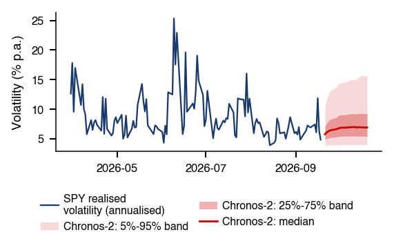
A stress episode shows how the forecasts react before any loss is averaged. In early April 2025, after the US (United States) tariff announcements, SPY realised volatility jumped on 4 April and peaked on 7 April. A one-day-ahead forecast made on the evening of 4 April can use the jump of that day, but not the news of the following days.
The interactive chart has dates on the horizontal axis and annualised volatility in per cent on the vertical axis. The thick line is the realised volatility, \(\sqrt{252\,\mathrm{RV}_t}\), and the thin lines are the one-day-ahead forecasts of log-HAR, GARCH-t, Chronos-2 and TimesFM-2.5; the other models can be switched on in the legend. The slider moves a 6-month window through the test period, and the ▶ button runs through it.
Question for the room Which initially displayed model anticipated the magnitude of the SPY realised-volatility peak on 7 April 2025?
Answer
None. Realised volatility reached 106.7% annualised. Forecasts for that day were 27.5% for log-HAR, 29.9% for GARCH-t, 30.1% for Chronos-2 and 30.4% for TimesFM-2.5. They had already risen from the previous day, after the jump of 4 April (46.3%), but underestimated the peak more than threefold. Heavy tails and pre-training do not supply the information in tariff news not yet observed.
In February–July 2025, the realised volatility peaked at 106.7% per year on 7 April 2025. No model anticipated the jump of 4 April, when the volatility reached 46.3%. The forecasts for 7 April rise after that jump, to 27.5% for log-HAR, 29.9% for GARCH-t, 30.1% for Chronos-2 and 30.4% for TimesFM-2.5, but all of them underestimate the peak more than threefold. One-day forecasts extrapolate the past, and the shock came from news not yet observed; neither heavy tails nor pretraining supply that information.
After the shock, the foundation models and log-HAR decay back at similar speeds. GARCH-t reacts to daily returns rather than to RV and decays more slowly.
In brief
SPY realised volatility (annualised) and one-day-ahead forecasts, February–July 2025
Peak 107% p.a. on 07.04.2025, after the United States tariff announcements
No model anticipates the jump on 04.04.2025 (46% p.a.)
Forecasts for 07.04.2025 rise after this jump, to 27–30% p.a.
All underestimate that day's 107% peak
One-day forecasts extrapolate the past, shocks come from news
Foundation models and log-HAR decay back at similar speeds
GARCH-t reacts to daily returns and decays more slowly
The central result of the chapter compares the mean QLIKE losses (14.20) of the eight models over the test period. The comparison is made twice: over the full test period and over the post-release window, when none of the foundation models could have seen the data in pretraining.
The interactive chart has two panels of horizontal bars, one per model, with the mean loss on the horizontal axis; a shorter bar is better. The left panel covers the test period from the date set with the slider, the right panel only the days after 3 November 2025. The selector switches the loss between QLIKE and the MSE, and the ▶ button moves the start of the left panel.
Question for the room Over the 979 SPY test days, what does the two-sided DM test at 5% establish about Chronos-2 versus log-HAR under QLIKE?
Answer
Mean QLIKE is 0.223 for Chronos-2 and 0.226 for log-HAR, but the DM p-value is 0.539. The descriptive advantage does not establish statistical superiority, and non-rejection does not establish equivalence. After 3 November 2025, the small LSTM has the lowest observed mean, 0.217; this is a sample ranking.
Over the full period of 979 days, Chronos-2 has the lowest mean QLIKE, 0.223, and log-HAR has 0.226. The DM test of Chronos-2 against log-HAR gives \(p\) = 0.539: the descriptive advantage does not establish superiority, and the non-rejection does not establish equivalence. After 3 November 2025, over 218 days, the small LSTM has the lowest mean loss, 0.217; this is a ranking in one sample.
and the test needs its moments to be finite, so the forecasts must also stay away from zero. Chronos-2 (0.223), Chronos-Bolt, TimesFM-2.5 and log-HAR (0.226) are not significantly different in the DM tests; for Chronos-2, \(p\) = 0.539.
The model confidence set (MCS) of Hansen, Lunde & Nason (2011) considers all models at once. Starting from the full set, it tests whether all models have equal average losses and, if this is rejected, drops the worst model; it repeats until equality is no longer rejected. The remaining models form a set that contains the best model with a given probability, here 90%. The 90% MCS keeps six of the eight models: only the random walk and GARCH-t are eliminated.
Two further results qualify the ranking. HAR in levels over-forecasts: its mean forecast is 1.35 times the mean of RV. After the release, the small LSTM is best (0.217), so the rankings are unstable across periods. What the result supports is a comparison of procedures: the zero-shot foundation models are not distinguished from the econometric benchmark. The full table with the DM and MCS \(p\)-values is in the Appendix.
In brief
Bars are average QLIKE losses
Left: full test period (979 days)
Right: after 3 November 2025 (218 days)
Chronos-2 (0.223), Chronos-Bolt, TimesFM-2.5 and log-HAR (0.226): DM tests not significant
Chronos-2 \(p\) = 0.539
DM and MCS need finite moments of the differential \(d_t = \mathrm{RV}_t(1/h_{A,t} - 1/h_{B,t}) + \ln(h_{A,t}/h_{B,t})\), so also forecasts that do not approach zero
The DM test asks whether two models have equal average losses. The test of Giacomini & White (2006) asks a conditional question: can the loss differential be predicted from yesterday's information? If it can, one model is better in some identifiable states, even when the average difference is zero. With instruments \(1\) and \(d_{t-1}\),
where \(d_t\) is the QLIKE loss of the model minus that of log-HAR, \(\bar Z\) is the mean of \(Z_t\) over the \(n\) forecasts and \(\hat\Omega\) the long-run variance of \(Z_t\). The null hypothesis is \(E[d_t] = 0\) and \(E[d_{t-1} d_t] = 0\) jointly. The variance \(\hat\Omega\) is a HAC estimate with a Bartlett kernel and 6 lags, because \(E[Z_t] = 0\) does not rule out autocorrelation in \(Z_t\); the test needs this long-run variance to be finite and non-singular.
The \(p\)-values are 0.828 for Chronos-2 and 0.812 for TimesFM-2.5: we do not reject the null, and no conditional difference from log-HAR is detected. A difference that is not detected is not proof of equality; the power of such tests is examined in the section on AI for scientific discovery.
In brief
Giacomini–White test (Giacomini & White (2006)): can the loss differential \(d_t\) be predicted from yesterday's information?
The forecast (14.21) uses the mean of RV computed from the grid. The simpler alternative is the exponential of the median, \(\exp(q_{0.5})\). The choice matters because of a theorem: QLIKE is consistent for the mean (Gneiting, 2011). The forecast \(h\) that minimises its expected value given the information \(\mathcal{F}\) is the conditional mean,
Monotone maps preserve quantiles, not means. The exponential of the median of log RV is therefore the median of RV, a functional elicited by the absolute error, not by QLIKE. If RV is lognormal and \(s^2\) is the variance of log RV, the ratio of median to mean is \(e^{-s^2/2} < 1\), so the median systematically under-forecasts the mean, the side that QLIKE penalises more.
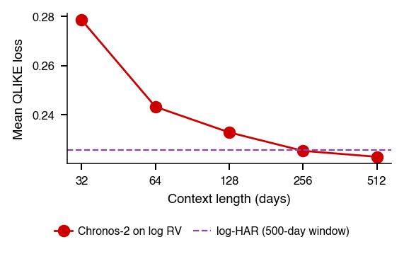
The table confirms this. With the grid mean, Chronos-2 has QLIKE 0.223 and its forecast averages 1.02 times the mean of RV; TimesFM-2.5 has 0.225 and 0.94. With the median, the QLIKE rises to 0.249 and 0.250, and both forecasts average 0.80 times the mean of RV. The median version is significantly worse (DM +3.53 for Chronos-2) and also worse than log-HAR (0.226). How the tail rule of the grid mean and the context length affect the result is shown in Further Topics.
In brief
Chronos-2 and TimesFM-2.5 on log RV
QLIKE
Mean forecast / mean RV
Chronos-2, \(\int_0^1 \exp(q_u)\,du\)
0.223
1.02
Chronos-2, \(\exp(q_{0.5})\)
0.249
0.80
TimesFM-2.5, \(\int_0^1 \exp(q_u)\,du\)
0.225
0.94
TimesFM-2.5, \(\exp(q_{0.5})\)
0.250
0.80
A theorem (Gneiting (2011)): QLIKE is consistent for the mean
The forecast \(h\) that minimises its expected value given the information \(\mathcal{F}\) is the conditional mean, \(\arg\min_h E[L(\mathrm{RV}, h) \mid \mathcal{F}] = E[\mathrm{RV} \mid \mathcal{F}]\)
Monotone maps preserve quantiles: \(\exp(\text{median of } \log \mathrm{RV})\) is the median of RV, elicited by absolute error (it minimises its mean), not by QLIKE
Lognormal RV, \(s^2\) the variance of log RV: median/mean \(= e^{-s^2/2}\)
The median version is significantly worse (DM +3.53 for Chronos-2) and worse than log-HAR (0.226)
For realised variance, the zero-shot foundation models are not distinguished from log-HAR: Chronos-2 has the lowest mean QLIKE over the full test period, but the difference is not significant, the MCS keeps six of eight models, and the GW (Giacomini–White, test) test finds no conditional difference. The result depends on reading the mean, not the median, from the quantile grid.
Test 3: VaR 1% and ES 2.5%
The third test moves from the centre and the scale of the distribution to its lower tail. It asks whether foundation models give better forecasts of VaR 1% and ES 2.5% than filtered historical simulation, either directly from their quantile grid or as volatility filters inside FHS. The evaluation combines the backtests of Chapter 8 for the breach sequence, tests of the whole predictive distribution, and a consistent loss for the pair (VaR, ES). It ends with a recalibration method that corrects the quantiles of a model after each breach.
Design of the Tail-Risk Test (1/2): Question and Targets
The targets are \(\mathrm{VaR}_\alpha\) and \(\mathrm{ES}_\alpha\) of (14.14), computed from the conditional quantiles \(q_u(r_{t+1} \mid \mathcal{F}_t)\), the \(u\)-quantile of tomorrow's return given today's information \(\mathcal{F}_t\); the definitions are on the frame From a Quantile Grid to VaR and ES. Two levels are used, each tied to a regulatory standard. VaR 1% is the level of the Basel backtesting rules, which rest on coverage tests. The pair (VaR 2.5%, ES 2.5%) corresponds to the ES level of the Fundamental Review of the Trading Book (FRTB).
The classical models are historical simulation (HS), which takes the empirical quantile of past returns; GARCH(1,1) with Student-\(t\) innovations; and filtered historical simulation (FHS) of McNeil & Frey (2000). All are estimated on a 1,000-day window and re-estimated every 20 days.
FHS is the benchmark because it combines a conditional GARCH volatility with the empirical shape of the tails, without assuming a distribution for the standardised returns. It reacts to volatility like GARCH, and it takes the tail shape from the data like HS.
In brief
Question: do foundation models give better VaR 1% and ES 2.5% forecasts than FHS?
Either directly or as volatility filters
Targets: VaR\(_\alpha\) and ES\(_\alpha\), computed from the quantiles \(q_u(r_{t+1} \mid \mathcal{F}_t)\)
The foundation models enter the test in two ways. The raw version takes the quantiles of tomorrow's return directly from the Chronos-2 grid, with a context of 512 returns. The hybrid version uses the foundation model only for the scale: it reads the series of absolute returns \(|r|\), with the 512 absolute returns before day \(t\) as context, and its forecast of \(|r_t|\) becomes the scale \(\hat\sigma_t\) (the grid mean for Chronos-2, the median for TimesFM). FHS is then applied to \(r_t/\hat\sigma_t\): the VaR is the empirical quantile of the standardised returns times \(\hat\sigma_t\).
Whether the scale is a median or a mean matters little here, unlike in Test 2, because FHS is scale-free. Multiplying the scale by a constant \(c > 0\) leaves the VaR unchanged:
A functional of a distribution is elicitable if some loss function is minimised, in expectation, by its true value: the mean by the squared error, a quantile by the pinball loss (14.2). ES alone is not elicitable, so there is no loss that compares ES forecasts on their own. The pair (VaR, ES), however, is jointly elicitable (Fissler & Ziegel, 2016), and forecasts of the pair can be ranked by a loss.
The chapter uses the zero-homogeneous Fissler–Ziegel loss, FZ0, of Patton, Ziegel & Chen (2019). With the daily loss \(L_t = -r_t\), a VaR forecast \(v\) and an ES forecast \(e > 0\) at tail level \(\alpha\),
where \(\mathbf{1}\{L_t > v\}\) equals 1 on a breach day. Lower values are better. The first term penalises breaches in proportion to their size relative to ES, and \(\log e\) penalises forecasts that are wider than needed.
Models are compared with DM tests on FZ0 differences and with the model confidence set of Test 2.
In brief
A functional is elicitable if some loss is minimised, in expectation, by its true value
The first check of a VaR forecast is its unconditional coverage: the share of days with a loss above the VaR should equal the level. The Kupiec test of Chapter 8 is a likelihood-ratio (LR) test of this hypothesis, with \(x\) breaches in \(T\) days:
Too many breaches indicate undercoverage, a VaR that is not extreme enough; too few indicate a VaR that is wider than needed.
The interactive chart shows, for each market on the horizontal axis, the breach rate of VaR 1% of each model on a log scale on the vertical axis. The light-blue band is the 95% range of the breach rate if the model were correct, and the dashed line marks 1%. The slider moves the start of the evaluation from 2016 to the post-release window, and the ▶ button runs through the start years.
Question for the room Raw Chronos-2 quantiles give 45 breaches of VaR 1% over 2,693 S&P 500 days. Does the Kupiec test at a nominal 5% level reject a 1% breach probability?
Answer
Yes. The Kupiec p-value is approximately 0.001. Under independent breaches with probability 1%, the nominal central 95% binomial range is [17, 37]; the 45 breaches (a rate of 1.67%) exceed it. More breaches indicate undercoverage, not conservatism. The range is discrete, and the Kupiec critical value is asymptotic. Used as a volatility filter for FHS, the same model gives 0.93% (p = 0.71).
Raw Chronos-2 has too many breaches on the S&P 500: 45 breaches in 2,693 days, a rate of 1.67%, with Kupiec \(p\) = 0.001. Under independent breaches with probability 1%, the nominal central 95% binomial range is 17 to 37 breaches, and 45 lies above it. On the BET the raw rate is 1.50%. Chronos-Bolt, whose lowest quantile of 10% is used as its "VaR 1%", is breached on 13.5% of the days.
The hybrids have breach rates close to 1% in all three markets; on the S&P 500, FHS with Chronos-2 volatility has 0.93% (\(p\) = 0.71). This checks average coverage only. The full table is in the Appendix.
In brief
Share of days with a loss above VaR 1% (log scale)
Light-blue band: 95% range if the model were correct
Kupiec (Chapter 8): likelihood-ratio (LR) test that the breach rate equals \(\alpha\), \(\chi^2_1\)
Raw Chronos-2: too many breaches on the S&P 500 (1.67%, Kupiec \(p\) = 0.001) and the BET (1.50%)
Chronos-Bolt, lowest quantile 10% used as “VaR 1%”: 13.5%
Hybrids: breach rates close to 1% in all three markets
The crash of February–June 2020 on the S&P 500 is the hardest episode of the test sample for a VaR model. Volatility rose within days, and a model that adjusts its scale slowly is breached repeatedly; a model that adjusts too strongly produces a VaR far above the losses that occur.
The interactive chart has dates on the horizontal axis and the loss in per cent on the vertical axis. The bars are the daily losses, with gains set to zero; the lines are the VaR 1% forecasts of FHS, raw Chronos-2 and FHS with Chronos-2 volatility, and the dots mark breaches. The other models can be switched on in the legend. The slider moves a 5-month window through the test period, and the ▶ button runs through it.
Question for the room In February–June 2020, FHS and the hybrid FHS with Chronos-2 volatility each have two breaches. Is that count sufficient to compare their forecast quality?
Answer
No. Both have 2 breaches over 104 days, but different paths: the highest VaR 1% is 58.9% for the hybrid (17.03.2020) and 26.4% for FHS, and the largest observed daily loss is 12.8%. These values motivate evaluating calibration and forecast loss. Neither equal breach counts nor VaR exceeding the largest realised loss establishes a ranking by itself. Raw Chronos-2 has 4 breaches, HS 12.
Over the 104 days of February–June 2020, FHS has 2 breaches, raw Chronos-2 4, FHS with Chronos-2 volatility 2 and HS 12. All models are hit in the first days of the crash. Chronos-2 reads the context fast, so its quantiles widen quickly.
The hybrid overshoots: its VaR 1% reaches 58.9% on 17 March 2020, against at most 26.4% for FHS and a largest daily loss of 12.8% (Appendix). FHS and the hybrid have the same number of breaches but very different paths, so the breach count alone does not rank them; that requires calibration tests and a forecast loss.
In brief
S&P 500, February–June 2020 (104 days): daily losses and VaR 1% forecasts
Dots: breaches
Breaches: FHS 2, raw Chronos-2 4, FHS with Chronos-2 volatility 2, HS 12
All models are hit in the first days
Chronos-2 reads the context fast, so its quantiles widen quickly
The hybrid overshoots: VaR 1% of 58.9% on 17.03.2020
Against 26.4% for FHS and a largest loss of 12.8% (Appendix)
A VaR with the right breach rate can still be wrong conditionally: breaches may come in clusters, on the days after a first breach, when the model has not yet adjusted. The independence test of Christoffersen (1998) models the breach indicator as a first-order Markov chain and tests, with an LR statistic that is \(\chi^2_1\) under the null, that a breach today does not change the probability of one tomorrow. Combined with the Kupiec statistic, it gives the test of conditional coverage, \(\chi^2_2\).
The dynamic quantile (DQ) test of Engle & Manganelli (2004) asks more generally whether breaches are predictable from past information:
where \(I_t = 1\) on a breach day. Under correct conditional coverage \(\mathrm{Hit}_t\) has mean zero and is uncorrelated with anything known at \(t-1\); the test is a Wald statistic that all six coefficients in (14.28) are zero, distributed as \(\chi^2_6\).
The table gives the \(p\)-values of the independence and DQ tests. On the S&P 500, the hybrids have the right breach rate but fail independence (\(p\) = 0.021 and 0.029) and DQ (\(p\) = 0.001 and below 0.001), and every model fails DQ at 5%. On the BET, FHS passes both tests (\(p\) = 0.409 and 0.650), while the hybrids fail DQ (\(p\) below 0.001). Being right on average is not being right conditionally. Further Topics shows where the decile grid of the other two models suffices, at VaR 10%.
In brief
\(p\): indep. / DQ
HS
GARCH-t
FHS
Chronos-2 raw
FHS + Chronos-2
FHS + TimesFM
S&P 500
0.001 / \(<\)0.001
0.205 / 0.001
0.045 / 0.021
0.223 / \(<\)0.001
0.021 / 0.001
0.029 / \(<\)0.001
Bitcoin
0.611 / 0.760
0.261 / 0.463
0.220 / 0.092
0.404 / 0.034
0.026 / 0.004
0.261 / 0.182
BET
0.399 / \(<\)0.001
0.258 / 0.082
0.409 / 0.650
0.270 / 0.026
0.475 / \(<\)0.001
0.379 / \(<\)0.001
Independence (Christoffersen (1998)): LR test that a breach today does not change the chance of one tomorrow
Backtests of VaR examine one quantile. The probability integral transform (PIT) (Diebold, Gunther & Tay, 1998) examines the whole predictive distribution. It is the forecast probability of a return at or below the one realised:
\[u_t = \hat F_t(r_t).\]
(14.29)
If the predictive distribution function \(\hat F_t\) is correct, the \(u_t\) of (14.29) are i.i.d. uniform on \((0, 1)\). A histogram of the \(u_t\) therefore shows where the forecast distribution is too narrow or too wide: a bar above its expected height means too many outcomes in that region.
The interactive chart has three panels, for the S&P 500, Bitcoin and the BET. The horizontal axis is the PIT \(u = \hat F(r)\), and the vertical axis the ratio of observed to expected frequency in each of the 22 intervals defined by the levels of the Chronos-2 grid; the dashed line at 1 is a correct forecast. The slider moves the start of the evaluation, and the ▶ button runs through the start years.
Question for the room On the S&P 500, how often does the realised return fall below the Chronos-2 1% quantile?
Answer
On 1.67% of the days, so the first PIT bar is 1.67 times its expected height: undercoverage at the 1% quantile. This frequency alone does not describe the shape of the whole tail. FHS gives 1.11%. The Berkowitz test rejects Chronos-2 on the S&P 500 (p = 0.019, σ̂ = 1.03); in the reported full-period tests, FHS is not rejected on any of the three markets.
On the S&P 500, the realised return falls below the Chronos-2 1% quantile on 1.67% of the days, so the first bar is 1.67 times its expected height: undercoverage at the 1% quantile. FHS gives 1.11%. This frequency alone does not describe the shape of the whole tail; the tests on the next frame use all the PIT values.
In brief
PIT (Probability Integral Transform) \(u_t = \hat F_t(r_t)\): the forecast probability of a return at or below the one realised (Diebold, Gunther & Tay (1998))
If the predictive distribution function \(\hat F_t\) is correct, the \(u_t\) are i.i.d. uniform on \((0, 1)\)
Bars: observed over expected frequency in the 22 intervals of the Chronos-2 grid
A bar above 1 means too many outcomes in that region
The test of Berkowitz (2001) turns the PIT into a Normal variable, \(z_t = \Phi^{-1}(u_t)\), where \(\Phi^{-1}\) is the standard Normal quantile function. If the forecast is correct, \(z_t\) follows the standard Normal distribution, and the test is an LR test of \(\mu = 0\) and \(\sigma = 1\), where \(\mu\) and \(\sigma\) are the mean and standard deviation of \(z_t\); values outside \([1\%, 99\%]\) are censored. An estimate \(\hat\sigma > 1\) means that the forecast tails are too thin. Chronos-2 is rejected on the S&P 500 (\(p\) = 0.019, \(\hat\sigma\) = 1.03) and on the BET; FHS is never rejected.
Calibration is one property; sharpness is another. The quantile score (QS) measures both, as the average pinball loss over the \(K\) levels \(u_k\) of the grid:
where \(q_{u_k}\) is the forecast quantile at level \(u_k\); lower values are better. The score (14.30) is a grid analogue of the continuous ranked probability score (CRPS) of Gneiting & Raftery (2007).
On the S&P 500 and the BET, Chronos-2 is worse than FHS both in the centre and in the tails; on the S&P 500 the DM statistics are +2.51 and +3.65. On Bitcoin the difference is not significant. The table for the three markets is in the Appendix.
In brief
Berkowitz test (Berkowitz (2001)): transform \(z_t = \Phi^{-1}(u_t)\), standard Normal if the forecast is correct
Test \(\mu = 0\), \(\sigma = 1\) for \(z_t\), censored outside \([1\%, 99\%]\)
\(\Phi^{-1}\): standard Normal quantile function; \(\mu\), \(\sigma\): mean and standard deviation of \(z_t\); \(\hat\sigma > 1\): tails too thin in the forecast
Chronos-2 rejected on the S&P 500 (\(p\) = 0.019, \(\hat\sigma\) = 1.03) and the BET; FHS never
Quantile score (QS): the average pinball loss over the \(K\) levels \(u_k\) of the grid
The FZ0 loss (14.26) ranks the forecasts of the pair (VaR 2.5%, ES 2.5%), and the MCS of Test 2 identifies the models that cannot be separated from the best. A model in the 90% set has not been shown to be worse than the others; several models can remain in the set without being equivalent.
The interactive chart is a table of MCS \(p\)-values for the FZ0 loss, with the models in rows and the markets in columns. Darker green means a higher \(p\)-value, and a cross marks a model eliminated at the chosen level. The slider moves the start of the evaluation, the selector sets the MCS level (75%, 90% or 95%), and the ▶ button runs through the start years.
Question for the room Over the three markets’ full test windows, which models does the 90% MCS eliminate, using FZ0 for VaR and ES at 2.5%?
Answer
Only HS on the BET has an MCS p-value below 0.10: it is 0.015. An MCS can retain several models without establishing that they are equivalent. On the S&P 500 FHS has the lowest FZ0 loss, and the DM test, Holm-adjusted over the five comparisons with FHS, separates FHS from the Chronos-2 hybrid (DM +2.65, p = 0.008 before the correction, Holm p = 0.032). On the BET the same test gives Holm p = 0.054.
Over the full test windows, the only model eliminated from the 90% set (\(p < 0.10\)) is HS on the BET, with \(p\) = 0.015. The FZ0 table is in the Appendix.
On the S&P 500, FHS has the lowest FZ0. The hybrids have the right breach rate but a larger VaR: over the 2,693 test days, the average VaR 1% is 3.20% for the Chronos-2 hybrid against 2.78% for FHS. Breach clustering does not separate them from FHS, since FHS and each hybrid have 2 back-to-back breaches. The family of tests is fixed in advance as the five DM tests against FHS on each market, with the Holm correction. On the S&P 500, FHS beats the Chronos-2 hybrid (DM +2.65, \(p\) = 0.008 before the correction, Holm \(p\) = 0.032). On the BET, DM is +2.36 with Holm \(p\) = 0.054, so superiority is not established at 5%. Over the 15 tests of the three markets, the Holm \(p\)-values are 0.096 and 0.180. What the result supports is a comparison of procedures.
In brief
\(p\)-values of the 90% model confidence set (Hansen, Lunde & Nason (2011)) for the FZ0 loss (darker green: higher)
The only model eliminated (\(p < 0.10\)) is HS on the BET (\(p\) = 0.015, the near-white cell)
The post-release window removes weight contamination but leaves few observations. After 3 November 2025, the S&P 500 has 220 days, Bitcoin 320 and the BET 217, so the expected numbers of VaR 1% breaches are 2.2, 3.2 and 2.2. The observed counts in the table range from 0 to 5. The weights used were public before 3 November 2025: the Hugging Face revision is pinned and identified by its SHA-256 (Secure Hash Algorithm, 256 bits) hash.
The power of the Kupiec test on such a window is low. With the asymptotic \(\chi^2_1\) cut-off at the nominal 5% level, and the power computed exactly from the binomial distribution against a true breach rate of 1.67%, the power is 0.19 at \(T = 220\) days. The actual size, the rejection rate when the model is right, is 0.13. The power rises to 0.50 at \(T = 1{,}000\) and 0.87 at \(T = 2{,}693\). A power of 80% is first reached at about 2,130 days, 8.4 years, and holds for good from 2,320 days; against a true rate of 2%, the power at \(T = 220\) is 0.29 (exercises A2 and A9 of Seminar 14).
Low power is not zero power. HS has 0 breaches on the S&P 500 after the release, and \(x = 0\) is in the Kupiec rejection region at \(T = 220\). For the other models, a non-rejection on this window does not establish calibration.
The weights used were public before 3.11.2025 (pinned Hugging Face revision, SHA-256 hash), but the tests have little power
Kupiec rule with the asymptotic \(\chi^2_1\) cut-off (nominal 5%), power computed exactly from the binomial, against a true rate of 1.67%: 0.19 at \(T = 220\) days
Actual size (rejection rate when the model is right) 0.13; power 0.50 at \(T = 1{,}000\); 0.87 at \(T = 2{,}693\)
80% power first at about 2 130 days (8.4 years), for good from 2 320
Against 2%: power 0.29 at \(T = 220\) (Seminar 14, exercises A2 and A9)
Low power is not zero power
HS has 0 breaches on the S&P 500, and \(x = 0\) is in the Kupiec rejection region at \(T = 220\)
The raw Chronos-2 quantiles are breached too often. A model-free correction shifts the model's quantile by the error it made recently and adapts the level after each breach. Define the score \(E_t = \hat q_{\alpha,t} - r_t\), where \(\hat q_{\alpha,t}\) is the model's \(\alpha\)-quantile for day \(t\);\(E_t > 0\) means that the return fell below it. The corrected quantile is \(\hat q_{\alpha,t} - \hat Q_{1-\alpha_t}\), where \(\hat Q_{1-\alpha_t}\) is the empirical \((1-\alpha_t)\) quantile of the last 250 scores.
Adaptive conformal inference (ACI) of Gibbs & Candès (2021) updates the level \(\alpha_t\) after every day:
In (14.31),\(\alpha\) is the target level, 1%, \(\mathrm{err}_t = 1\) on a breach, and \(\gamma > 0\) is the step size, here 0.001. After a breach \(\alpha_t\) falls by \(\gamma(1-\alpha)\), so the next VaR is wider; after a calm day it rises by \(\gamma\alpha\), slowly. With \(\gamma = 0\) the method becomes a rolling calibration at a fixed level, with the correction recomputed daily from the last 250 scores; this is not standard split conformal prediction.
The guarantee of ACI concerns the long-run average of \(\mathrm{err}_t\), which converges to \(\alpha\) whatever the data, not the value of \(\alpha_t\) on any day. Its derivation is in Further Topics.
In brief
Idea: shift the model's quantile by the error it made recently
\(\alpha\): target level (1%); \(\mathrm{err}_t = 1\) on a breach
\(\gamma > 0\): step size, here 0.001; \(\gamma = 0\): rolling calibration at a fixed level (the correction is recomputed daily from the last 250 scores), not standard split conformal
After a breach \(\alpha_t\) falls (the next VaR is wider); after a calm day it rises slowly
The chart applies (14.31) to the raw Chronos-2 quantiles and compares the corrected VaR 1% with the raw one and with FHS. The top panel shows the level \(\alpha_t\), which the method moves around the target of 1%; the bottom panel shows the three VaR series.
The interactive chart has dates on the horizontal axis. The top panel has the adaptive level \(\alpha_t\) in per cent, with a dashed line at the 1% target; the bottom panel has VaR 1% in per cent on a log scale, for raw Chronos-2, Chronos-2 with ACI and FHS. The first selector chooses the market, the slider the step \(\gamma\) (0, where the method is rolling calibration at a fixed level, to 0.005), and the second selector the number of calibration days (125, 250 or 500). The ▶ button runs through the step sizes.
Question for the room For the S&P 500, with γ = 0.001 and 250 calibration days, how does the average conformal VaR 1% compare with that of FHS over the same days?
Answer
It is higher: 3.36% for the conformal correction and 2.85% for FHS over 2,443 days, although the breaches are 21 against 24.4 expected. Breach rates close to the target do not imply equal averages. Separately, the joint VaR–ES comparison at 2.5% gives mean FZ0 losses of 1.205 and 1.013, with DM p = 0.001; this does not follow from average VaR 1% alone. With γ = 0 (rolling calibration at a fixed level) there are 16 breaches and an average VaR of 3.58%.
On the S&P 500, with \(\gamma\) = 0.001 and 250 calibration days, the corrected VaR has 21 breaches over 2,443 days, against 24.4 expected. Its average VaR 1% is 3.36%, against 2.85% for FHS on the same days: breach rates close to the target do not imply equal average VaR. With \(\gamma = 0\) there are 16 breaches and the average VaR is 3.58%.
The top panel shows that the adaptive level \(\alpha_t\) stays mostly above 1%. The shift of the scores alone would make the VaR too wide: with \(\gamma = 0\), rolling calibration at a fixed level, there are 16 breaches and the average VaR 1% is 3.58%. ACI compensates by loosening the level.
The bottom panel compares the VaR 1% of raw Chronos-2, Chronos-2 with ACI and FHS, on a log scale. ACI brings the breaches near 1%: on the S&P 500, 21 against 24.4 expected, and conditional coverage is not rejected in any market. The DQ test still rejects on the S&P 500 and the BET. The corrected VaR is wider: over the 2,443 days after the 250 calibration days, its average VaR 1% is 3.36% against 2.85% for FHS on the same days, and its FZ0 is significantly higher.
What the result supports is a comparison of procedures: ACI against raw Chronos-2 and against FHS. Proper scoring rules reward sharpness subject to calibration (Gneiting & Raftery, 2007). ACI repairs calibration, but calibration is necessary, not sufficient; on the same days, FHS has the narrower VaR and the lower FZ0.
In the tail, raw Chronos-2 has too many VaR 1% breaches on the S&P 500 and the BET and fails the Berkowitz test. Used as a volatility filter inside FHS, it gives the right breach rate but a wider VaR, and FHS keeps the lowest FZ0 loss on the S&P 500. The post-release window is too short to test VaR 1% with useful power, and recalibration by ACI fixes coverage at the cost of sharpness.
Case Studies: The Virtue of Complexity and the M6 Competition
The two case studies place the chapter's tests in the recent literature. The first, Kelly, Malamud & Zhou (2024), argues theoretically and empirically that return-prediction models with more parameters than observations can do better out of sample, a case for the large models of this chapter against the parsimony rule of classical econometrics. The second, the M6 competition of Makridakis et al. (2025), is a live out-of-sample test of whether any forecasting method beats equal probabilities in ranking asset returns. Both are replicated on the course data.
Case Study: Is Complexity a Virtue in Return Prediction? (1/2)
Kelly, Malamud & Zhou (2024) ask two questions. Must a return-prediction model have far fewer parameters \(P\) than observations \(T\)? And can models with complexity \(c = P/T > 1\) do better out of sample? The setting, in equations 1–2 of the paper, is that next month's return is an unknown function of today's predictors, approximated by a wide network:
In (14.32),\(R_{t+1}\) is the market excess return, \(G_t\) the vector of predictors known at \(t\) and \(\varepsilon_{t+1}\) the unpredictable part. Each \(S_{i,t}\) is a non-linear feature of \(G_t\), a hidden unit of a network with one hidden layer, and \(\beta_i\) its weight. By universal approximation (Hornik, Stinchcombe & White, 1989), the sum approaches \(f\) as \(P\) grows.
The question matters for this chapter because the models tested in it have far more parameters than any financial series has observations. Classical econometrics prescribes parsimony; the paper gives a theoretical case for the opposite.
The link to Test 1 is direct. There, no model beats the zero forecast on the S&P 500 and Bitcoin after the correction for multiple testing. The paper asks whether a negative out-of-sample \(R^2\) means that a forecast has no economic value. Economic value is measured by the Sharpe ratio of the market-timing return \(\pi_t R_{t+1}\), with position \(\pi_t = \hat\beta' S_t\) (equation 6 of the paper), where \(\hat\beta\) are the estimated weights and \(S_t\) the vector of the \(P\) features at \(t\). The forecast itself is the position.
The theory, in Sections III–IV of the paper, shows that for a misspecified model with optimally chosen ridge shrinkage, and under the assumptions of the paper, the expected out-of-sample \(R^2\) and the timing Sharpe ratio rise with \(c\). Near \(c = 1\), the interpolation boundary, least squares fits the training data exactly and its variance explodes. Beyond it, as \(c\) grows further, performance recovers.
In brief
Link to Test 1: no model beats the zero forecast on the S&P 500 and Bitcoin
After the multiple-testing correction
The paper asks whether a negative out-of-sample \(R^2\) means no economic value
Economic value: Sharpe ratio of the market-timing return \(\pi_t R_{t+1}\), with position \(\pi_t = \hat\beta' S_t\) (eq. 6)
The forecast itself is the position
\(\hat\beta\): estimated weights; \(S_t\): vector of the \(P\) features at \(t\)
Theory (Sections III–IV): expected out-of-sample \(R^2\) and timing Sharpe ratio rising with \(c\)
For a misspecified model with an optimally chosen ridge penalty \(z\) (shrinks the weights \(\hat\beta\) towards zero), under the assumptions of the paper
Near \(c = 1\) (the interpolation boundary) least squares fits the training data exactly and its variance explodes
The data, in Section V.A of the paper, are the monthly excess returns of the value-weighted index of the Center for Research in Security Prices (CRSP), 1926–2020. The predictors are the 15 of Welch & Goyal (2008), 14 variables and the lagged market return. Returns are scaled by their trailing 12-month volatility, predictors by an expanding-window standard deviation, and 36 months of warm-up move the start of the sample to 1930.
The features are random Fourier features (RFF; equation 20 of the paper, Rahimi & Recht (2007)):
Each feature in (14.33) is a sine or a cosine of a random combination of the predictors. The vector \(\omega_i\) is drawn once from the standard Normal distribution, with \(I\) the identity matrix, and then fixed; \(\gamma\) sets the degree of non-linearity, and a larger \(\gamma\) gives faster oscillating features. The model is a wide two-layer network whose first-layer weights are random; only the output weights \(\beta\) are estimated, by ridge regression with penalty \(z\).
\(P\) counts columns: \(P/2\) vectors \(\omega_i\), each giving a sine and a cosine, so \(P = 12{,}000\) uses 6,000 vectors. The ridge estimator and the design are detailed in Further Topics.
In brief
Data (Section V.A): monthly excess return of the CRSP value-weighted index, 1926–2020
CRSP: Center for Research in Security Prices
The 15 predictors of Welch & Goyal (2008) (14 variables and the lagged market return)
Returns scaled by their trailing 12-month volatility, predictors by an expanding-window standard deviation
36 months of warm-up, so the sample starts in 1930
Table I, Panel A of the paper reports the results for a training window of \(T = 12\) months. The information ratio is measured against the market, the maximum loss is the largest monthly loss in standard deviations, and the \(t\)-statistics test the mean strategy return (Sharpe column) and the alpha (information-ratio column).
The ridgeless kitchen sink, a linear model with all 15 predictors and \(P = 15 > T = 12\), has an \(R^2\) below −100% and a Sharpe ratio of −0.11. At the interpolation boundary the forecasts explode, which reproduces the negative verdict of Welch & Goyal (2008). With the same predictors and a penalty \(z = 10^3\), the \(R^2\) is −3.8%, yet the Sharpe ratio is 0.46 (\(t\) = 4.4). The \(R^2\) penalises the scale of the forecasts, whereas timing profits depend on their correlation with returns (footnote 5 of the paper).
The RFF model with \(c = 1{,}000\) has an information ratio of 0.26 (\(t\) = 2.5) against the best linear model. With \(T\) = 60 and 120 months its information ratios against the market are 0.25 and 0.24 (\(t\) = 2.3 and 2.2; Panels B–C). Non-linearity extracts more from the same predictors, with a smaller maximum loss and positive skewness.
The positions (Figure 10 of the paper) are almost always long and are cut before 14 of the 15 recessions dated by the National Bureau of Economic Research (NBER), out of sample. The model learns the sign restriction of Campbell & Thompson (2008) without being given it. What the result supports is a comparison of procedures: models of different complexity, out of sample.
In brief
Model (\(T = 12\))
\(R^2\) (%)
Sharpe [\(t\)]
Inf. ratio [\(t\)]
Max loss
Skewness
Linear, \(z = 0^+\)
\(<-100\)
\(-0.11\) [\(-1.0\)]
\(-0.16\) [\(-1.6\)]
\(98.5\)
\(-0.9\)
Linear, \(z = 10^3\)
\(-3.8\)
\(0.46\) [\(4.4\)]
\(0.33\) [\(3.1\)]
\(2.4\)
\(-0.1\)
RFF, \(c = 1\,000\), \(z = 10^3\)
\(0.6\)
\(0.47\) [\(4.5\)]
\(0.31\) [\(2.9\)]
\(1.2\)
\(2.5\)
Source: Table I, Panel A, of the paper; information ratio against the market; maximum monthly loss in standard deviations; the \(t\)-statistics test the mean strategy return (Sharpe column) and alpha (information-ratio column)
Kitchen sink (all predictors), no ridge penalty (\(P = 15 > T = 12\) months): \(R^2\) below \(-100\%\), Sharpe ratio \(-0.11\)
Reading: at the interpolation boundary forecasts explode, reproducing the negative verdict of Welch & Goyal (2008)
Same predictors with \(z = 10^3\): \(R^2 = -3.8\%\), yet Sharpe ratio \(0.46\) (\(t = 4.4\))
Reading: \(R^2\) penalises the scale of forecasts; timing profits depend on their correlation with returns (footnote 5)
RFF, \(c = 1\,000\): information ratio \(0.26\) (\(t = 2.5\)) against the best linear model
With \(T\) = 60 and 120, \(0.25\) and \(0.24\) against the market (\(t\) = \(2.3\) and \(2.2\); Panels B–C)
Reading: nonlinearity extracts more from the same predictors, with a smaller maximum loss and positive skewness
Positions (Figure 10): almost always long
Cut before 14 of 15 NBER (National Bureau of Economic Research) recessions, out of sample
The chart replicates Figures 7–8 of Kelly, Malamud & Zhou (2024) on the course data: SPY excess returns with 7 predictors, \(T = 12\) complete observations, \(\gamma = 2\) and 1,000 draws of the random features, over 354 test months from February 1997 to August 2026.
The interactive chart has two panels with the complexity \(c = P/T\) on a log scale on the horizontal axis and one line per ridge penalty \(z\). The left panel shows the out-of-sample \(R^2\) in per cent, clipped at −60%, or, with the selector, the mean squared norm \(\lVert\hat\beta\rVert^2\) of the ridge estimate; the right panel shows the annualised Sharpe ratio of the timing strategy. The dotted line in the right panel is the linear model with the 7 predictors and \(z = 10^3\). The first slider chooses the highlighted penalty, the second moves the cursor along \(c\), and the ▶ button runs through the complexities.
Question for the room With the penalty fixed at z = 10³, how does the Sharpe ratio of the RFF timing strategy evolve over the tested grid from c = 1 to c = 1,000?
Answer
It rises to c = 50, then falls: 0.12 at c = 1, the grid maximum of 0.26 at c = 50 and 0.11 at c = 1,000 (t = 0.6). The linear model with the same 7 predictors and z = 10³ has 0.32. This is a result for the stated penalty and sample, not a general rule about complexity.
With the penalty fixed at \(z = 10^3\), the Sharpe ratio is 0.12 at \(c = 1\), rises to the maximum of the grid, 0.26, at \(c = 50\), and falls to 0.11 at \(c = 1{,}000\)(\(t\) = 0.6). The linear model with the same 7 predictors and \(z = 10^3\) has 0.32. This is a result for the stated penalty and sample, not a general rule about complexity.
Nearly ridgeless, with \(z = 10^{-3}\), the out-of-sample \(R^2\) is −1,852% at \(c = 1\) and recovers to −16.6% at \(c = 1{,}000\). This is the double descent of Figure 7 of the paper: the error peaks at the interpolation boundary and falls again beyond it. The left panel is cut at −60% to keep the other curves visible. The data are described in the Appendix.
With \(z = 10^3\) the Sharpe ratio is 0.12 at \(c = 1\), 0.26 at \(c = 50\) and 0.11 at \(c = 1{,}000\)(\(t\) = 0.6). The linear model with \(z = 10^3\) has a Sharpe ratio of 0.32 (\(t\) = 1.7) and is not beaten by RFF. The \(t\)-statistic tests the mean strategy return, \(\sqrt{n}\,\bar R/s_R\), not the Sharpe ratio itself; with HAC errors (Newey–West with 3, 6 and 12 lags), it is 1.75, 1.81 and 1.81. The information ratio of RFF is 0.07 against the linear model (\(t\) = 0.4) and −0.12 against SPY.
On the course data, complexity helps up to \(c \approx 50\), not up to \(c = 1{,}000\). What the result supports is a comparison of procedures. How the positions relate to recessions is shown in Further Topics.
The authors state the limits of their results. The theory is for linear ridge models on fixed random features and a single asset; a panel with cross-asset covariances is left open (Introduction, footnote 2). Predictability is assumed to be spread evenly across features (Assumption 4), and sparse models of the LASSO (Least Absolute Shrinkage and Selection Operator) type are left to future research (footnote 22). There is no optimal degree of non-linearity \(\gamma\). The average timing returns are about half as large in 1975–2020 as in 1930–1974 (Section V.F).
The course data are smaller: 7 of the 15 predictors and about 30 years (exercise C3 of Seminar 14). With them, the power of a two-sided 5% test for an information ratio of 0.31 is only about 39%, since the expected \(t\)-statistic is \(0.31\sqrt{29.5} \approx 1.7\). A failure to replicate on such a sample is weak evidence against the paper.
The open question is whether learned features can replace random ones: for example, the embeddings of a pretrained foundation model such as Chronos-2 as \(S_t\). Whether complexity is still a virtue with such features, on a panel of the course markets, is not known.
In brief
Limits stated by the authors
Theory for linear ridge models on fixed random features and a single asset
A panel with cross-asset covariances is left open (Introduction, footnote 2)
Predictability spread evenly across features (Assumption 4)
Sparse LASSO-type (Least Absolute Shrinkage and Selection Operator) models left to future research (footnote 22)
No optimal degree of nonlinearity \(\gamma\)
Average timing returns about half as large in 1975–2020 as in 1930–1974 (Section V.F)
Course data (Seminar 14, exercise C3): 7 of the 15 predictors and about 30 years
The power of a two-sided 5% test for an information ratio of 0.31 is only about 39% (\(t \approx 0.31\sqrt{29.5} \approx 1.7\))
Open question: learned instead of random features
The embeddings of a pretrained foundation model such as Chronos-2 as \(S_t\)
Is complexity still a virtue, on a panel of course markets?
Makridakis et al. (2025) ask whether a forecasting method, however complex, can beat equal probabilities in forecasting the relative performance of assets. M6 was a live competition in 2022–2023, with 226 teams and 100 assets, 50 S&P 500 stocks and 50 international ETFs. The task was to give, for each asset, the probability that its four-week return falls in each of the five quintiles of the universe. Teams used machine learning, time-series models and their own judgment.
The competition matters for this chapter because it is an out-of-sample evaluation in real time: the forecasts were submitted before the outcomes existed, so it is free of contamination through pretraining. Forecasts are scored by the ranked probability score (RPS), defined on the frame on the replication.
The main claim is that equal probabilities are hard to beat. Of the 163 teams of the global leaderboard, 38 (23.3%) have an RPS below the benchmark's 0.16, and only 3 beat it in all 12 months. The 11 teams that beat the benchmark in both forecasting and investing reduce the RPS by at most 2.2%. Among the top 20% of teams by RPS, 14 use machine learning and 12 time-series models (Table 7 of the paper). The correlation between the RPS and the information ratio (IR) of the team's portfolio is 0.04 (\(p\) = 0.601), over the 138 teams whose forecasts differ from the benchmark.
In brief
Question (Makridakis et al. (2025)): can a forecasting method, however complex, beat equal probabilities in forecasting the relative performance of assets?
M6: a live competition, 2022–2023, 226 teams, 100 assets (50 S&P 500 stocks and 50 international ETFs)
The task: the probability that the four-week return of each asset falls in each of the five quintiles of the universe
Why it matters: an out-of-sample evaluation in real time, hence free of contamination through pretraining
Teams used machine learning, time-series models and their own judgment
Main claim: equal probabilities are hard to beat
Of the 163 teams of the global leaderboard, 38 (23.3%) have an RPS (ranked probability score) below the benchmark's 0.16; only 3 beat it in all 12 months
The 11 teams that beat the benchmark in both forecasting and investing reduce the RPS by at most 2.2%
Among the top 20% of teams by RPS, 14 use machine learning and 12 time-series models (Table 7)
The correlation between the RPS and the information ratio (IR) of the team's portfolio is 0.04 (\(p\) = 0.601), over the 138 teams whose forecasts differ from the benchmark
The chart applies the M6 task to the 19 M6 assets in the course data and compares three models with equal probabilities. The models and the adaptation are described on the next frame; the result is read here.
The interactive chart has two panels. The left panel shows, as bars, the RPS reduction over equal probabilities in per cent, in the 12 M6 periods and in the 93 four-week periods from 26 July 2019 to 11 September 2026; the dotted line is the median M6 team (RPS 0.162, computed in the paper over 162 of the 163 teams; 100 assets), a context marker and not a comparable threshold. The right panel shows the cumulative RPS reduction period by period, with the blue area marking the competition year. The slider sets the confidence \(w\) in the forecast, from 0 (equal probabilities) through 1 (the model) to 2, and the ▶ button runs through it.
Question for the room With w = 1, which of the three models has the lowest mean RPS over the 93 periods of 2019–2026, on the 19 M6 assets of the course data?
Answer
The volatility-only model. RPS reductions relative to equal probabilities are 2.33% for it (DM −6.35, p < 0.001), 0.81% for the historical mean (p = 0.358) and 1.72% for the network (p = 0.016). Volatile assets get larger probabilities for the extreme quintiles. The ranking does not follow from using means or from model complexity, and it changes with w: at w = 0.5 the historical mean gains 1.91%, slightly above the volatility model (1.88%); at w = 2 the volatility model gains only 0.28%.
With \(w = 1\), the model that uses only volatility has the largest RPS reduction over the 93 periods: 2.33% (DM −6.35, \(p\) < 0.001), against 0.81% for the historical mean (\(p\) = 0.358) and 1.72% for the network (\(p\) = 0.016). Volatile assets receive larger probabilities for the extreme quintiles. The ranking changes with \(w\): at \(w = 0.5\) the historical mean gains 1.91%, slightly above the volatility model (1.88%), and at \(w = 2\) the volatility model gains only 0.28%.
In brief
Left: RPS reduction over equal probabilities (%), in the 12 M6 periods and in 93 four-week periods (26.07.2019–11.09.2026); dotted line: the median M6 team (RPS 0.162, computed in the paper over 162 of the 163 teams; 100 assets), a context marker, not a comparable threshold
Right: the cumulative RPS reduction, period by period; the blue area marks the competition year
The ranked probability score (equation 1 of the paper) is the distance between the forecast and the realised cumulative distribution over the quintiles:
where \(f_{ik}\) is the forecast probability that asset \(i\) falls in quintile \(k\), and \(q_{ik}\) is, in M6, 1 for the realised quintile and 0 otherwise. With 19 assets, quintiles cannot hold equal numbers of assets, so \(q_{ik}\) is the share of quintile \(k\) covered by the asset's rank interval \([(r-1)/19,\, r/19]\), a fractional weight. With 100 assets, equal probabilities (\(f_{ik} = 0.2\)) give an RPS of 0.16; with the fractional weights used here, 0.1516. Because (14.34) compares cumulative probabilities, a forecast that misses by one quintile costs less than one that misses by four.
The adaptation uses the 19 M6 assets present in the course data: AMZN (Amazon.com, Inc., Nasdaq ticker), JPM (JPMorgan Chase & Co., NYSE ticker), META (Meta Platforms, Nasdaq ticker), HYG (iShares iBoxx High Yield Corporate Bond ETF), IEF (iShares 7–10 Year Treasury Bond ETF), IWM (iShares Russell 2000 ETF), LQD (iShares iBoxx Investment Grade Corporate Bond ETF), SHY (iShares 1–3 Year Treasury Bond ETF), TLT (iShares 20+ Year Treasury Bond ETF) and the 10 XL* sector ETFs, with total returns computed from adjusted prices. The four-week M6 calendar (Table 1 of the paper) is extended back to 2019.
Three models are compared. The historical-mean model simulates Normal returns with the mean and covariance of the last 250 days, 20,000 times. The volatility-only model uses a zero mean and the exponentially weighted moving average (EWMA) covariance with \(\lambda = 0.94\). The network has 4 inputs (volatilities and returns over 20 and 250 days), 8 neurons and 5 output probabilities; it is trained with the RPS as the loss and re-estimated each year on the periods since 2004.
In brief
RPS (eq. 1): the distance between the forecast and the realised cumulative distribution over the quintiles
\(f_{ik}\): forecast probability that asset \(i\) falls in quintile \(k\); \(q_{ik}\) (M6 notation, not a quantile here): in M6, 1 for the realised quintile and 0 otherwise
Here, with 19 assets: the share of quintile \(k\) covered by the asset's rank interval \([(r-1)/19,\, r/19]\) (fractional weights)
With 100 assets, equal probabilities (\(f_{ik} = 0.2\)) give an RPS of 0.16; with the fractional weights here, 0.1516
Adaptation: the 19 M6 assets in the course data (AMZN, JPM, META, HYG, IEF, IWM, LQD, SHY, TLT and the 10 XL* sector ETFs), total returns from adjusted prices
The four-week M6 calendar (Table 1), extended from 2019; with 19 assets the realised quintiles are fractional
Historical mean: Normal returns with the mean and covariance of the last 250 days, 20,000 simulations
Volatility only: zero mean and the EWMA covariance (exponentially weighted moving average, \(\lambda = 0.94\))
The network: 4 inputs (volatilities and returns over 20 and 250 days), 8 neurons, 5 probabilities; RPS as the loss, re-estimated each year on the periods since 2004
The volatility-only model beats the benchmark: its RPS is 2.7% lower in the M6 year, in 11 of the 12 periods, and 2.3% lower since 2019 (DM −6.35, \(p\) < 0.001). The 2.7% here and the 2.2% of the paper come from different universes and targets and are not directly comparable. The mechanism is visible in the first M6 period: META, with an EWMA volatility of 76% a year, has a probability of 0.82 of landing in an extreme quintile, HYG, with 7%, has 0.08, and the benchmark gives 0.40.
The historical mean lowers the RPS by 1.9% in the M6 year but only by 0.8% since 2019 (\(p\) = 0.358). With the same 250-day covariance, a zero mean has an RPS 1.7% lower than the estimated mean (DM −1.75, \(p\) = 0.080). The network raises the RPS by 1.4% in the M6 year and lowers it by 1.7% since 2019 (\(p\) = 0.016). Against the volatility-only model, its RPS is 0.6% higher, a difference that is not detected (DM 0.73, \(p\) = 0.466); without the return inputs, its RPS rises by only 0.05% (\(p\) = 0.70).
What the result supports is a comparison of procedures. As in Tests 1 and 2, the useful information is in the dispersion of returns, not in their sign. The limits are clear: 19 assets instead of 100, and one market. Because the RPS is bounded, the DM test needs no assumption on the tails. In the paper the evaluation covers a single year, and only 26 of the 163 teams submitted new forecasts at all 12 deadlines; and the periods before 2022 use, with hindsight, the universe chosen for M6.
In brief
The volatility-only model beats the benchmark: an RPS lower by 2.7% in the M6 year (11 of 12 periods) and by 2.3% since 2019 (DM \(-\)6.35, \(p < 0.001\))
2.7% here and 2.2% in the paper come from different universes and targets, so they are not directly comparable
The mechanism: in the first M6 period, META (EWMA volatility 76% a year) has a probability of 0.82 of landing in an extreme quintile, HYG (7%) 0.08, the benchmark 0.40
The historical mean lowers the RPS by 1.9% in the M6 year but only by 0.8% since 2019 (\(p\) = 0.358)
With the same 250-day covariance, a zero mean has an RPS 1.7% lower than the estimated mean (DM \(-\)1.75, \(p\) = 0.080)
The network raises the RPS by 1.4% in the M6 year and lowers the RPS by 1.7% since 2019 (\(p\) = 0.016)
Against the volatility-only model: an RPS 0.6% higher, a difference not detected (DM 0.73, \(p\) = 0.466)
Without the return inputs the RPS rises by only 0.05% (\(p\) = 0.70)
Type of evidence: comparison of procedures; the useful information is in the dispersion of returns, not in their sign, as in Tests 1 and 2
Limits: 19 assets, not 100, and one market
The RPS is bounded, so the DM test needs no assumption on the tails
In the paper: a single year, and only 26 of the 163 teams submitted new forecasts at all 12 deadlines
The periods before 2022 use, with hindsight, the universe chosen for M6
The complexity case study shows that a large model can have economic value with a negative out-of-sample \(R^2\), but on the course data the gain stops at moderate complexity and the linear model is not beaten. The M6 replication shows that in ranking assets the useful signal is dispersion, which a zero-mean volatility model captures without any network.
AI for Scientific Discovery
The tests of the chapter leave one result unexplained: on SPY realised variance, a model pretrained on mostly non-financial series is not distinguishable from log-HAR. The section turns this into a research question, skill or memory, and shows how an AI assistant can help at each step of the research loop, and where its proposals must be checked. The mini-case tests the assistant's typical answer and finds that the available data cannot decide it.
Open Question: Forecasting Skill or Memorisation of Training Data?
Test 2 found that zero-shot Chronos-2 is not distinguishable from log-HAR on SPY realised variance. Other evidence points the other way for returns: Rahimikia, Ni & Wang (2025) find that off-the-shelf foundation models do poorly on daily excess returns across global markets, both zero-shot and after fine-tuning, while models pretrained from scratch on financial data gain. And Lopez-Lira, Tang & Zhu (2025) show that once a model has seen the realised values, its counterfactual forecasting skill is not identified: detected memorisation is only a lower bound. Their argument is made for LLMs, but the logic applies to any pretrained forecaster.
Two open questions follow. Is the parity with log-HAR learned structure, such as long memory and mean reversion, or recall of the test period? And can a short post-release window tell the two apart?
A test can be built from the loss differential of Test 2,
the QLIKE loss \(L\) of the foundation model (FM) minus that of log-HAR. Memorisation implies \(E[d_t \mid \text{post}] > E[d_t \mid \text{pre}]\): the FM loses its edge after the release of its weights. The null hypothesis is equality. A rejection could also reflect a change of market regime at the same date.
In brief
Test 2: zero-shot Chronos-2 is not distinguishable from log-HAR on SPY realised variance
Rahimikia, Ni & Wang (2025): on daily excess returns across global markets, off-the-shelf foundation models do poorly
Zero-shot and after fine-tuning
Models pretrained from scratch on financial data gain
Lopez-Lira, Tang & Zhu (2025): once a model has seen the realised values, its counterfactual forecasting skill is not identified
Detected memorisation is only a lower bound
Shown for LLMs; the logic applies to any pretrained forecaster
Open questions
is the parity learned structure (long memory, mean reversion) or recall of the test period?
Literature. An assistant can be asked for evaluations of time-series foundation models on financial data since 2024, but every arXiv identifier it returns must be checked, and the documentation of the pretraining corpora must be read directly.
Hypotheses: predictions that separate memorisation from skill, such as a comparison before and after the release, series that were never public, and simulated series with the same dynamics.
Data and code. From the chapter's volatility forecasts, the QLIKE differential of Chronos-2 minus log-HAR is computed, together with a pre/post test with HAC errors and its minimum detectable effect (MDE).
Robustness, fixed in advance: a placebo release date one year earlier must show no break, and simulated series, which cannot have been memorised, serve as a control.
Critique. The assistant is asked to attack the conclusion "no memorisation, because the post-release test is insignificant"; a good critique should point to low power and to the different regimes before and after the release.
Reusable prompts for the five steps are in the Appendix.
In brief
Literature: ask an assistant for evaluations of time-series foundation models on financial data since 2024
Check every arXiv identifier and read the corpus documentation yourself
Hypotheses: predictions that separate memorisation from skill
Pre vs post release, never-public series, simulated series with the same dynamics
Data and code: from the chapter's volatility forecasts, the QLIKE differential Chronos-2 minus log-HAR
A pre/post test with HAC errors and the minimum detectable effect (MDE)
Robustness, fixed in advance: a placebo release date one year earlier must show no break
Simulated series cannot be memorised
Critique: ask the assistant to attack “no memorisation, because the post-release test is insignificant”
A typical proposal of an assistant is that the parity of Chronos-2 comes from memorised data, so its edge over log-HAR must vanish after the release. The chart tests this with the differential (14.35), split at the release date.
The interactive chart has the mean QLIKE differential \(d_t\) on the horizontal axis, with a dashed line at zero. The first row is the mean before the break date, in green, the second the mean after it, in orange, each with its 95% HAC interval; the bottom row is the estimated change \(\hat\beta_1\), after minus before, with red marks at ±MDE, the smallest change the test detects with 80% power. The selector chooses the foundation model, the slider moves the break date, and the ▶ button runs the break date through the test period.
Question for the room For Chronos-2 on SPY, what does the performance comparison before and after 3 November 2025 establish about memorisation?
Answer
Neither its presence nor its absence. The estimated change in the QLIKE differential against log-HAR is +0.0074, with HAC t = 0.88 and p = 0.38. The MDE at 80% power is 0.0234, larger than the observed change; even an infinite post-release window would leave an MDE of 0.0157. Non-rejection does not rule out memorisation, and a significant change would not by itself distinguish memorisation from a change in market regime.
With the break on 3 November 2025, the mean \(d_t\) of Chronos-2 is −0.0045 over the 761 days before and +0.0029 over the 218 days after. The estimated change is +0.0074, with HAC \(t\) = 0.88 and \(p\) = 0.38, and the MDE at 80% power is 0.0234, larger than the observed change.
The chart reads as follows. The green and orange rows are the mean QLIKE differentials of Chronos-2 against log-HAR before and after the release, with 95% HAC intervals. The bottom row is the estimated change \(\hat\beta_1\), with red lines at ±MDE.
Before 3 November 2025, over 761 days, the mean \(d_t\) is −0.0045: Chronos-2 has a slightly lower loss than log-HAR. After it, over 218 days, the mean is +0.0029. The change is +0.0074, with HAC \(t\) = 0.88 and \(p\) = 0.38, so we do not reject equality. The test needs a finite long-run variance of \(d_t\), and therefore forecasts that do not approach zero.
What the result supports is association, not causation. Even a rejection would tie the difference only to the release date, not to memorisation: anything else that changed at that date would produce the same pattern.
In brief
Typical assistant proposal: “the parity of Chronos-2 comes from memorised data, so its edge must vanish after release”
Chart: mean QLIKE differential \(d_t\) (Chronos-2 minus log-HAR) before and after the release
Green: before; orange: after
With 95% HAC intervals
Bottom row: the estimated change \(\hat\beta_1\), with red lines at \(\pm\)MDE
MDE: the smallest effect the test can detect
Mean \(d_t\): \(-\)0.0045 before 3 Nov 2025 (761 days), +0.0029 after (218 days)
Change +0.0074, HAC \(t\) = 0.88, \(p\) = 0.38
The test needs a finite long-run variance of \(d_t\), so forecasts that do not approach zero
Type of evidence: association (the variables move together; this does not prove causation)
Even a rejection would tie the difference to the release date only, not to memorisation
where \(z_{0.975} = 1.96\) and \(z_{0.8} = 0.84\) are standard Normal quantiles, \(\hat\beta_1\) the estimated post-release shift in the mean of \(d_t\) and \(\mathrm{SE}_{HAC}\) its HAC standard error. The MDE is 5.3 times the pre-release gap, and it would still be 0.0157 with an infinite post-release window.
The floor comes from the structure of the standard error. HAC errors give each period its own long-run variance \(V\), and
More post-release days remove only the second term of (14.37), leaving an MDE of \(2.80\sqrt{V_{pre}/761}\). Waiting does not solve the problem.
"No memorisation" is therefore not a finding of this test. Power must come from the cross-section, many series tested at once, not from waiting for a longer window. The pitfalls a researcher must check are listed in Further Topics.
The project asks where memorisation is impossible: does the zero-shot skill for daily variance survive after the release, on simulated series and on less-covered markets? The first step is to replicate the chapter's numbers: the mean QLIKE of log-HAR (0.226) and of Chronos-2 (0.223), the DM \(p\)-value of 0.539 and the 218-day post-release window.
The deliverables are:
a pre-registered power calculation;
a panel of series from the course data, with a range-based variance proxy and a loss that is robust to the proxy (Patton, 2011);
pre/post tests with placebo release dates and the MCS across models;
a referee-style critique with a reply.
Each prompt that shaped a decision is logged in `AI_USE.md`, and each invented reference, leak or wrong number that was caught goes in `AI_ERRORS.md`, with the test that caught it. Templates are in the project folder.
In brief
Questions (where memorisation is impossible)
does zero-shot skill for daily variance survive after release?
does it survive on simulated series?
does it survive on less-covered markets?
Replicate first: the chapter's QLIKE of log-HAR (0.226) and Chronos-2 (0.223)
DM \(p\) = 0.539
The 218-day post-release window
Deliverables
A pre-registered power calculation
A panel of series from the course data with a range-based variance proxy and a proxy-robust loss (Patton (2011))
Pre/post tests with placebo release dates; the MCS across models
A referee-style critique and your reply
Log each prompt that shaped a decision in AI_USE.md
Each invented reference, leak or wrong number caught in AI_ERRORS.md, with the test that caught it
The parity of Chronos-2 with log-HAR cannot be attributed to skill or to memory with the data of the chapter: the post-release change is not significant, and the test could not have detected a change of the size observed. Answering the question requires many series, simulated series and pre-registered power, not a longer wait.
The architectures of the chapter address the problem of memory in different ways. The gates of the LSTM can mitigate vanishing gradients, but with a forget-gate bias of 0 the gradient still vanishes. Attention connects distant time steps directly. Foundation models forecast zero-shot from a context window and return quantiles, from which point, volatility and tail forecasts follow.
The three tests give three different answers. For returns, after the multiple-testing correction, nothing beats the zero forecast on the S&P 500 and Bitcoin. For volatility, the foundation models are not distinguishable from log-HAR. For the tails, they are useful only as volatility filters inside FHS.
The method generalises beyond these models. Every new model should be evaluated against a strong benchmark and after the release of its weights, with inference that matches the design: Clark–West for nested models, SPA or Romano–Wolf for many models, and the PIT, quantile scores and the DQ test for distributions. Further reading is listed in the Appendix.
In brief
LSTM gates can mitigate vanishing gradients
With a forget-gate bias of 0 they still vanish
Attention connects distant time steps directly
Foundation models forecast zero-shot from a context window and return quantiles
The three tests
Returns: after the multiple-testing correction, nothing beats zero on the S&P 500 and Bitcoin
Volatility: foundation models not distinguishable from log-HAR
Tails: FHS remains the benchmark; foundation models at most as volatility filters
Evaluate every new model against a strong benchmark and after the release of its weights
With inference that matches the design: Clark–West for nested models
Chapter 15 asks whether text read by a large language model can forecast returns or volatility. The same threats return, look-ahead, memorisation of the test period and weak benchmarks, and so do the same tools: post-release windows, the Clark–West test and control of multiplicity.
In brief
Retrieval questions
Why does a stable RNN forget at the rate of the VAR(1) impulse response \(A^k\), not necessarily like \(\rho(A)^k\)?
Why is \(\exp(q_{0.5})\) of log RV a biased forecast under QLIKE?
Why can a hybrid VaR pass Kupiec and still lose the FZ0 comparison?
Why is “not significant after release” not evidence against memorisation?
For daily index returns, the choice is the zero forecast. For realised volatility, it is log-HAR, with a zero-shot foundation model when thousands of series must be forecast without estimation. For VaR 1% and ES 2.5%, it is FHS, with a foundation model at most as a volatility filter or with conformal recalibration.
The conditions are those of the chapter's samples. On the S&P 500 and Bitcoin, no model beats the zero forecast after the multiple-testing correction; on the BET, the SPA \(p\)-value, Holm-corrected for the three markets, is 0.056. On SPY, Chronos-2 and log-HAR have QLIKE 0.223 and 0.226 (DM \(p\) = 0.539). On the S&P 500, FHS has the lowest FZ0 loss (DM +2.65 against the Chronos-2 hybrid).
The decision should be revisited if a model beats the zero forecast after Holm or SPA, in a test family fixed in advance; if a foundation model has a QLIKE significantly below log-HAR in the post-release window; or if a hybrid VaR passes the independence and DQ tests as well as Kupiec.
In brief
What I choose
Daily index returns: the zero forecast
Realised volatility: log-HAR; a zero-shot foundation model when thousands of series must be forecast without estimation
VaR 1% and ES 2.5%: FHS, with a foundation model at most as a volatility filter or with conformal recalibration
Under which conditions
On the S&P 500 and Bitcoin, no model beats the zero forecast after the multiple-testing correction
On the BET, the SPA \(p\)-value, Holm-corrected for the three markets, is 0.056
On SPY, Chronos-2 and log-HAR have QLIKE 0.223 and 0.226 (DM \(p\) = 0.539)
On the S&P 500, FHS has the lowest FZ0 loss (DM +2.65 against the Chronos-2 hybrid)
What result would make me drop it
A model that beats the zero forecast after Holm or SPA, in a test family fixed in advance
A foundation model with a QLIKE significantly below log-HAR in the post-release window
A hybrid VaR that also passes the independence and DQ tests, not only Kupiec
Section summary
Deep networks and foundation models add no value for the mean of daily index returns, are not distinguishable from log-HAR for realised variance, and are useful in the tail only inside FHS. The method of evaluation, strong benchmarks, post-release windows and inference matched to the design, carries over to the language models of the next chapter.
Further Topics
The frames in this part extend topics treated briefly in the body of the chapter: the vanishing gradient measured by automatic differentiation, a numerical example of attention with a causal mask, what Chronos sees of a return series, the Transformer block and the architectures built from it, a worked VaR and ES computation from a quantile grid, a zero-shot fan chart for volatility, the training and seed sensitivity of the LSTM, the stale prices behind the BET result, the tail rule of the grid mean, the context length, VaR 10%, the guarantee of adaptive conformal inference, the method and positions of the complexity case study, and the pitfalls a researcher must check.
The chart measures \(|\partial h_T/\partial x_{T-k}|\) by automatic differentiation, relative to its value at \(k = 0\), for networks with 16 hidden units averaged over 50 random initialisations and the same Normal inputs. The simple RNN keeps \(8.3 \times 10^{-5}\) at lag 20 and \(7.4 \times 10^{-9}\) at lag 50, so nothing is learned from inputs more than a few weeks back. The LSTM with forget-gate bias 0 is no better (\(1.2 \times 10^{-10}\) at lag 50), because \(f \approx 0.5\) halves the memory at every step, while with bias 3 it keeps 8.4% at lag 50, as predicted by \(0.953^{50} \approx 0.09\) in (14.8). The forget-gate bias should therefore be initialised at a positive value.
In brief
\(|\partial h_T / \partial x_{T-k}|\) by automatic differentiation, relative to \(k = 0\) as on the vertical axis
16 hidden units, 50 random initialisations, same Normal inputs
Simple RNN: \(8.3 \times 10^{-5}\) at lag 20, \(7.4 \times 10^{-9}\) at lag 50
Nothing is learned from inputs more than a few weeks back
LSTM, forget-gate bias 0: \(1.2 \times 10^{-10}\) at lag 50
No better than the RNN: \(f \approx 0.5\) halves the memory at every step
LSTM, bias 3: 8.4% at lag 50
As predicted by \(0.953^{50} \approx 0.09\)
Initialise the forget-gate bias at a positive value
With three time steps and \(d_k = 1\), queries \(q = (1, 0, 2)\), keys \(k = (0.5, 1, -1)\) and values \(v = (1, 2, 3)\), step 3 has scores \((1, 2, -2)\), softmax weights \((0.265, 0.721, 0.013)\) and output 1.75: it draws mostly on step 2, whose key matches its query best. A causal mask adds \(M_{tj} = -\infty\) for \(j > t\) to the scores, so that step \(t\) uses only steps \(j \le t\); step 1 then puts weight 1 on itself, whereas without the mask 57% of its weight would come from step 2, a later day. In a 512-day context every value is already observed at the forecast origin, so a model that reads only the context may attend in both directions; the mask matters where the model is trained to predict later positions from earlier ones.
The chart shows the last 512 S&P 500 daily returns after the mean scaling of (14.12) and the bins to which they are assigned. Scaling divides every return by the mean absolute return of the context, so the model sees a series free of units, and quantisation maps each scaled value to the nearest of 4,093 bin centres.
The scale of the context is \(s\) = 0.672%, the scaled returns range from −9.2 to 13.5, 96% of them lie within ±3, and the 512 returns use only 336 of the 4,093 tokens. Because scaling removes the units, the volatility level must be read from the context. When a crash day with return \(M\) (in per cent) enters the context and the oldest return \(x_{\text{out}}\) leaves it, \(s\) rises by \((|M| - |x_{\text{out}}|)/C\), approximately \(|M|/C\), percentage points; the relative rise, about \(|M|/(Cs)\), is large in a short context and small in a 512-day one (exercises A3 and A6 of Seminar 14).
In brief
Context: the last 512 S&P 500 daily returns
Scale \(s\) = 0.672%
Scaled returns from \(-\)9.2 to 13.5, 96% within \(\pm 3\)
The 512 returns use 336 distinct tokens out of 4,093
Scaling makes the model free of units, so the volatility level must be read from the context
A crash day with return \(M\) (in %) enters the context and the oldest return \(x_{\text{out}}\) leaves it
\(s\) rises by \((|M| - |x_{\text{out}}|)/C\) percentage points, approximately \(|M|/C\)
The relative rise, about \(|M|/(C s)\), is large in a short context and small in a 512-day one
A Transformer block (Vaswani et al., 2017) applies multi-head attention (MHA) and then a small MLP to each position separately, each part with a skip connection and layer normalisation (LN): \(Z = \mathrm{LN}(X + \mathrm{MHA}(X))\) and \(H = \mathrm{LN}(Z + \mathrm{MLP}(Z))\). Multi-head attention runs \(m\) attentions in parallel, each with its own \(W_Q\),\(W_K\),\(W_V\), concatenates them and projects the result with \(W_O\); layer normalisation standardises each row and rescales it with learned parameters. The skip connection \(X + \mathrm{MHA}(X)\) lets the gradient pass straight through the block, and a model stacks several blocks, with \(H\) as the input of the next.
In brief
Transformer block (Vaswani et al. (2017)): multi-head attention, then a small MLP applied to each position separately
\[
Z = \mathrm{LN}\big(X + \mathrm{MHA}(X)\big), \qquad H = \mathrm{LN}\big(Z + \mathrm{MLP}(Z)\big)
\]
Each part has a skip connection and a normalisation
\(\mathrm{MHA}(X) = [\mathrm{head}_1, \dots, \mathrm{head}_m]\,W_O\) (multi-head attention): \(m\) attentions in parallel, each with its own \(W_Q\), \(W_K\), \(W_V\), concatenated and projected by \(W_O\)
\(\mathrm{LN}\) (layer normalisation): each row is standardised, then rescaled by learned parameters
\(X + \mathrm{MHA}(X)\): the skip connection, which lets the gradient pass straight through the block
A model stacks several blocks: \(H\) is the input of the next block
The blocks are assembled in three ways. An encoder attends in both directions inside the context; Chronos-2 is encoder-only and returns the quantile grid in one pass (Ansari et al., 2025). A decoder-only model, such as TimesFM (Das et al., 2024), uses a causal mask and is trained to predict the next patch at every position. An encoder–decoder, such as the T5 of the original Chronos, reads the context with the encoder and writes the forecast one token at a time with the decoder. The original Chronos is trained with the cross-entropy, a classification over 4,093 bins,
while Chronos-2 uses the robust scaling \(\tilde x_t = \sinh^{-1}((x_t - \hat\mu)/\hat\sigma)\), with \(\hat\mu\) and \(\hat\sigma\) the mean and standard deviation of the context; \(\sinh^{-1}\) grows like a logarithm for large values and so damps outliers.
In brief
Three ways to assemble the blocks
Encoder: attention in both directions inside the context; Chronos-2 is encoder-only and returns the quantile grid in one pass (Ansari et al. (2025))
Decoder-only: causal mask, trained to predict the next patch at every position: TimesFM (Das et al. (2024))
Encoder–decoder (T5, used by the original Chronos): the encoder reads the context; the decoder writes the forecast one token at a time
Cross-entropy (original Chronos): predicting the next token is a classification over 4,093 bins
For the S&P 500 on 18 September 2026, with context up to 17 September, Chronos-2 gives \(q_{0.01} = -2.704\%\) and \(q_{0.05} = -1.400\%\), so VaR 1% is 2.704%. Linear interpolation gives \(q_{0.025} = q_{0.01} + \tfrac{0.015}{0.04}(q_{0.05} - q_{0.01}) = -2.215\%\), so VaR 2.5% is 2.215%. With \(q_u\) flat below 1% and the trapezoid rule between 1% and 2.5%, (14.14) gives \(\mathrm{ES}_{2.5\%} = 40 \times [0.01 \times 2.704 + 0.015 \times 2.459] = 2.56\%\). The ratio ES/VaR at 2.5% is 1.15, below the Normal value of 1.19, although this grid has a heavier left tail than the Normal: the flat tail below 1% understates ES (exercise A7 of Seminar 14).
In brief
Worked example, S&P 500, quantiles for 18.09.2026 (context up to 17.09.2026): \(q_{0.01} = \)\(-\)2.704%, \(q_{0.05} = \)\(-\)1.400%
VaR 1% \(=\) 2.704%
linear interpolation between the two levels: \(q_{0.025} = q_{0.01} + \frac{0.015}{0.04}(q_{0.05} - q_{0.01}) = \)\(-\)2.215%, so VaR 2.5% \(=\) 2.215%
ES 2.5%: \(q_u\) flat below 1%, trapezoid rule between 1% and 2.5%
The fan chart shows a Chronos-2 forecast of SPY volatility 22 trading days ahead from 18 September 2026, made zero-shot on log realised variance with a 512-day context. The line is the median and the two bands are the 5–95% and 25–75% quantile ranges, converted to annualised volatility.
The last realised volatility is 4.8% a year and its 20-day average 6.8%; the median forecast at 22 days is 6.9%, with a 90% band from 4.0% to 15.8%. The forecast reverts to the mean, as GARCH and HAR do (Chapters 5 and 9), with no estimation on SPY. The band is skewed upwards partly by construction, because volatility is \(\sqrt{252\,e^{q}}\) of a log-variance quantile \(q\) and a convex map stretches the upper side; but on the log-volatility scale, half the log variance, the band still lies 0.56 below and 0.82 above the median, so the model itself also leans towards spikes.
In brief
Chronos-2 on log realised variance of SPY (512-day context)
SPY: the exchange-traded fund (ETF) that tracks the S&P 500
22 trading days ahead from 18.09.2026
Bands: quantiles 5–95% and 25–75%
Last volatility 4.8% p.a., 20-day average 6.8%
Median forecast at 22 days 6.9%, 90% band 4.0–15.8%
Mean reversion, as in GARCH and HAR (Chapters 5, 9), with no estimation on SPY
The band is skewed upwards partly by construction: volatility is \(\sqrt{252\,e^{q}}\) of a log-variance quantile \(q\)
A convex map stretches the upper side
On the log-volatility scale (half the log-variance), the band still lies 0.56 below and 0.82 above the median, so the model itself also leans towards spikes
The chart shows the training and validation MSE of the return LSTM by epoch, on standardised S&P 500 returns for seed 0, with a dotted vertical line at the epoch whose weights are kept. Early stopping halts training when the validation MSE has not improved for a fixed number of epochs.
The LSTM reads the last 20 returns, standardised on the training period, with \(h = 16\) hidden units, one input per step and a linear output: \(4(hd + h^2 + 2h) + h + 1 = 1{,}233\) parameters, where the factor 4 counts the three gates and the candidate. It is trained once on up to 4,000 days, with the last 20% as the validation block, by MSE and Adam with weight decay \(10^{-4}\); training stops after 25 epochs without a lower validation MSE, and the forecast is the average of 5 seeds. On the S&P 500 training stops 26 epochs in and the weights of epoch 1 are kept, so the network has seen the data once and stays close to its random start, one reason why the seed matters; the validation MSE is lower than the training MSE mainly because the last years of the training period were calmer. There is little to learn: the standard deviation of the forecasts is 0.047%, against 1.13% for returns.
In brief
Input: the last 20 returns, standardised on the training period
\(h = 16\) hidden units, \(d = 1\) input per step, linear output
\(4(hd + h^2 + 2h) + h + 1\) = 1 233 parameters (4: the three gates and the candidate; \(2h\): two bias vectors per gate)
MSE, Adam, weight decay \(10^{-4}\)
Trained once on up to 4,000 days, the last 20% being the validation block
Early stopping: training stops after 25 epochs without a lower validation MSE (patience), and the best weights are kept
Forecast = average of 5 seeds
Chart (S&P 500, seed 0): training and validation MSE by epoch, on standardised returns
The dotted vertical line marks the epoch kept
Training stops 26 epochs in, and the weights of epoch 1 are kept
The kept network has seen the training data once and stays close to its random start: one reason why the seed matters
Validation MSE is lower than training MSE mainly because the last years of the training period were calmer
Little to learn: forecast s.d. 0.047% against 1.13% for returns
The chart plots, for each model, SSE(zero) − SSE(model) \(= \sum_{s \le t}[r_s^2 - (r_s - \hat r_s)^2]\), where SSE is the sum of squared errors in %²: the curve rises when the model beats the zero forecast and falls when it loses. All curves stay near zero in calm years and jump in March 2020, so one month decides the ranking. The AR(1) gains in 2020 from the negative autocorrelation of crash days and then gives part of the gain back, while TimesFM-2.5 loses steadily. The path should be reported together with the final \(R^2\).
The chart compares the out-of-sample \(R^2\) of five LSTMs that differ only in the random seed, and of their average. For single seeds the variation is as large as the effect: from −0.79% to +0.24% on Bitcoin and from +0.37% to +1.96% on the S&P 500. On the BET the result is robust, with all 5 seeds between +1.01% and +1.22%. Choosing the best seed after seeing the test is backtest overfitting (Chapter 13).
In brief
Out-of-sample \(R^2\) of five LSTMs that differ only in the random seed, and of their average
Single seeds: variation as large as the effect
Bitcoin: from \(-\)0.79% to +0.24%
S&P 500: from +0.37% to +1.96%
BET: robust across seeds
All 5 seeds between +1.01% and +1.22%
Choosing the best seed after seeing the test is backtest overfitting (Chapter 13)
Stale prices of thinly traded constituents make index returns positively autocorrelated even when every price is efficient (Lo & MacKinlay, 1990). Since 2016 the first-order autocorrelation is 0.06 for the BET and −0.14 for the S&P 500, and the LSTM forecast has a correlation of 0.88 with the previous day's BET return: it mostly learned this autocorrelation. On the BET-tracking ETF Patria-TVBETETF, over 2,629 common days, the same signal has a same-day \(R^2\) of 2.88% (1.26% for the BET on the same days), but the ETF is thinly traded too (autocorrelation 0.07, 4.2% of days with zero return). Executed one day later, the \(R^2\) is 0.57%, with Clark–West \(p\) = 0.003. The evidence is consistent with stale-price effects; a small signal survives the execution lag, before transaction costs (Chapter 2).
In brief
Stale prices of thinly traded constituents make index returns positively autocorrelated (Lo & MacKinlay (1990))
Even if every price is efficient
First-order autocorrelation since 2016: BET 0.06, S&P 500 \(-0.14\)
The LSTM forecast has correlation 0.88 with the previous day's BET return: it mostly learned this autocorrelation
Tradable check: the BET-tracking ETF Patria-TVBETETF, 2 629 common days, same LSTM signal
Same day: \(R^2\) 2.88% (BET 1.26% on the same 2 629 days)
But the ETF is thinly traded too (autocorrelation 0.07, 4.2% zero-return days)
Executed one day later: \(R^2\) 0.57%, Clark–West \(p\) = 0.003
Reading: the evidence is consistent with stale-price effects
A small signal survives the execution lag, before transaction costs (Chapter 2)
Take a toy grid with levels 25%, 50% and 75% and log-quantiles \(q = -1, 0, 1\), with target \(E[Y] = \int_0^1 e^{q_u}\,du\). Equal weights on the three points give 1.36 and the course rule (trapezoid, flat below 25% and above 75%) gives 1.41, while a Normal log \(Y\) with these quartiles, \(s = 1/z_{0.75} = 1/0.674 = 1.48\), has \(E[Y] = e^{s^2/2} = 3.00\): the flat tails miss more than half of it. Because \(\exp\) is convex and unbounded, the top of the distribution carries much of the mean, and truncating the upper tail can understate it badly, although the sign of the total error is not guaranteed. In Test 2, the mean forecast relative to mean RV is 1.02 for Chronos-2 (grid to 99%), 0.97 for Chronos-Bolt and 0.94 for TimesFM-2.5 (grids to 90%), consistent with a cut upper tail, though the forecasts themselves also differ. The rule should be reported with the forecasts.
A Normal log \(Y\) with these quartiles (\(s = 1/z_{0.75} = 1/0.674 = 1.48\), \(z_{0.75}\) the 75% standard Normal quantile) has \(E[Y] = e^{s^2/2}\) = 3.00
The flat tails miss more than half of it
Reading: \(\exp\) is convex and unbounded, so the top of the distribution carries much of the mean
Truncating the upper tail can understate the mean badly; the sign of the total error is not guaranteed (a flat lower tail raises the integral)
Test 2: mean forecast / mean RV is 1.02 for Chronos-2 (grid to 99%), 0.97 for Chronos-Bolt and 0.94 for TimesFM-2.5 (grids to 90%)
Consistent with a cut upper tail, though the forecasts themselves also differ
The chart shows the QLIKE of Chronos-2 on log RV with contexts from 32 to 512 days, on the same forecast days. The loss falls from 0.279 with 32 days to 0.223 with 512 days, and below about 256 days Chronos-2 is worse than log-HAR (0.226). Months of history reveal the slow-moving level of volatility, which HAR encodes explicitly through its 22-day average. The context length is a modelling choice to report and test, like a window length.
In brief
QLIKE of Chronos-2 on log RV with contexts of 32 to 512 days, on the same forecast days
QLIKE falls from 0.279 (32 days) to 0.223 (512 days)
Below about 256 days Chronos-2 is worse than log-HAR (0.226)
Long memory: months of history reveal the slow-moving level
HAR encodes it explicitly through its 22-day average
Context length is a modelling choice to report and test, like a window length
At the 10% level all three foundation models have a quantile in their grid, so the comparison is free of the extrapolation problem of VaR 1%. On the S&P 500 the breach rates of the 10% quantile are 9.8% for HS and 9.6% for FHS, against 11.7% for Chronos-2, 13.5% for Chronos-Bolt and 12.0% for TimesFM-2.5, and Kupiec rejects the foundation models in eight of the nine cases. Their lower tail sits too high, through location, scale or tail shape; a plausible reason is that the pretraining corpora are dominated by smoother series. As volatility filters inside FHS, the models inherit the tails from the data.
In brief
Breach rate of the 10% quantile (target 10%) for HS, FHS and the three foundation models
The bound shrinks like \(1/T\), so it is a long-run statement only, and it is loose for small \(\gamma\). For ES 2.5%, the Chronos-2 ES is shifted by the VaR 2.5% correction, a heuristic without a conformal guarantee; the rules and the full table are in the Appendix.
In brief
Guarantee for any sequence of returns, no model needed: over \(T\) days the breach rate approaches \(\alpha\)
where \(z > 0\) shrinks \(\hat\beta\) towards zero and \(z \to 0^+\) gives the ridgeless, pseudo-inverse solution. The design (Section V.C) uses rolling windows of \(T\) = 12, 60 and 120 months, \(P\) from 2 to 12,000 and \(\log_{10} z = -3, \ldots, 3\), with results averaged over 1,000 independent draws of the features. The out-of-sample \(R^2\) is \(1 - \mathrm{Var}(\text{error})/\mathrm{Var}(R)\) (footnote 40), while the theory divides the MSE by \(E[R^2]\), the zero forecast of Test 1; the strategies are evaluated by the annualised Sharpe ratio and by the alpha and information ratio from a regression of the timing return on the market, against the linear kitchen-sink regression on all 15 predictors (Section V.D).
The chart shows, on the course data, the timing position \(\hat\beta' S_t\) of the RFF model with \(c = 1{,}000\) and \(z = 10^3\), month by month, with its 6-month moving average in red and the NBER recessions shaded (series `USREC` from FRED, Federal Reserve Economic Data).
The position is long in 73% of the months, with an average of 0.13: a positive equity premium learned without a sign restriction. Its average is 0.05 in the 6 months before the 3 recessions of the sample and −0.01 during them, against 0.14 otherwise, and the 2020 pandemic shock is not anticipated. Three recessions are a description, not a test; the paper has 15 recessions and 90 years.
In brief
On course data, as in Kelly, Malamud & Zhou (2024): position \(\hat\beta' S_t\) of RFF with \(c = 1\,000\), \(z = 10^3\)
Shaded: NBER recessions (series USREC from FRED, Federal Reserve Economic Data)
Red: 6-month moving average
Long in 73% of months, average position 0.13
A positive equity premium learned without a sign restriction
Average position 0.05 in the 6 months before the 3 recessions and \(-0.01\) during them
Against 0.14 otherwise
The 2020 pandemic shock is not anticipated
Three recessions are a description, not a test: the paper has 15 recessions and 90 years
Five pitfalls recur in the evaluation of new forecasting models:
Leakage comes from pretraining overlap, full-sample scaling or HAR averages that include day \(t\); in exercise B10 of Seminar 14 these cut QLIKE by a quarter, and the test is a post-release window, simulated or private series, and recomputing the forecast for \(t\) from data truncated at \(t-1\).
Weak benchmarks are avoided by comparing with zero for returns, log-HAR for volatility and FHS for the tails, not with a random walk.
The wrong functional means medians used as means or deciles used as 1% quantiles; the mean forecast relative to mean RV should be near 1, and for the Chronos-2 median it is 0.80.
Selection of seeds, contexts and models after seeing the test is controlled by logging every trial and comparing the whole set with the MCS.
Wrong inference means DM on nested models, no multiplicity control, coverage without independence, or "not significant" reported without the MDE.
In brief
Leakage: pretraining overlap, full-sample scaling, HAR averages that include day \(t\)
Seminar 14, exercise B10: they cut QLIKE by a quarter
Test: post-release window, simulated or private series
Recompute the forecast for \(t\) from data truncated at \(t-1\)
Weak benchmarks: compare with zero (returns), log-HAR (volatility), FHS (tails), not with a random walk
Wrong functional: medians used as means; deciles used as 1% quantiles
Mean forecast / mean RV should be near 1; Chronos-2 median: 0.80
Selection: seeds, contexts and models chosen after seeing the test
Log every trial, compare the whole set with the MCS
The appendix contains the derivations and complete tables to which the body of the chapter refers: norms, spectral radius and explosion in recurrent networks, the fit of geometric against hyperbolic decay, other foundation models and their corpora, a formal protocol for contamination, the full tables of the three tests, the COVID-19 overshoot, the Berkowitz tests and quantile scores, the rules of conformal recalibration, the data of the complexity replication, and the prompts of the discovery loop.
The condition \(\gamma_\varphi \lVert W\rVert_2 < 1\) of (14.6) is sufficient for geometric vanishing, so \(\gamma_\varphi \lVert W\rVert_2 \ge 1\) is necessary for explosion (Pascanu, Mikolov & Bengio, 2013). In a linear RNN, a spectral radius \(\rho(W) > 1\) is necessary for exponential explosion, and \(\rho(W) = 1\) with a Jordan block, a repeated eigenvalue without a full set of eigenvectors, still gives polynomial growth; with a non-linear \(\varphi\) the local Jacobians \(D_t W\) matter, and \(\rho(W) = 0\) with \(\rho(DW) > 1\) is possible. In a stable VAR the impulse responses, and with them the gradients, decay asymptotically like \(\rho(A)^k\), up to a factor \(k^{m-1}\) for a Jordan block of size \(m\), but at finite horizons \(\lVert A^k\rVert_2\) can exceed 1: \(A = \left(\begin{smallmatrix} 0.5 & 4 \\ 0 & 0.5 \end{smallmatrix}\right)\) has \(\rho(A) = 0.5\), yet \(\lVert A^2\rVert_2 \approx 4.0\). The term \(DUx_t\) in (14.7) is an innovation only if the inputs are centred white noise; long-memory inputs would pass through the network.
In brief
\(\gamma_\varphi \lVert W\rVert_2 < 1\) is sufficient for geometric vanishing, so \(\gamma_\varphi \lVert W\rVert_2 \ge 1\) is necessary for explosion (Pascanu, Mikolov & Bengio (2013))
With constant gates, an i.i.d. candidate input \(g_t\) and a stationary start, the LSTM cell has \(\operatorname{Corr}(c_t, c_{t-k}) = f^k\), whereas an autoregressive fractionally integrated moving average (ARFIMA) process with \(0 < d < 1/2\) has \(\rho_k \sim C k^{2d-1}\). For S&P 500 absolute returns since 2000 the autocorrelation is 0.289 at lag 1 and 0.132 at lag 50. A geometric decay with its own amplitude, \(\rho_k = \rho_1 f^{k-1}\), the autocorrelation of an AR(1) signal observed with noise, matches both lags with \(f\) = 0.984, that is \(b_f\) = 4.1 and a half-life of 43 days; but that \(f\) implies 0.027 at lag 150, while the data show 0.059, more than twice as much. A constant gate \(f < 1\) is a short-memory filter, and a long context or explicit long averages, as in HAR, only approximate long memory over a finite range of lags.
Chronos-2 is trained on selected Chronos and GIFT-Eval (General Time Series Forecasting Model Evaluation, benchmark GIFT-Eval) datasets plus synthetic multivariate series and is benchmarked on GIFT-Eval (Aksu et al., 2024) and fev-bench; the TimesFM corpus contains Google Trends, Wikipedia page views and synthetic series, as well as the series of the M4 forecasting competition, electricity, traffic and weather. According to the Hugging Face repositories, the updated weights of TimesFM-2.5 were announced on 15 September 2025 and released on 1 October 2025, and those of Chronos-2 announced on 20 October 2025 and released on 30 October 2025. The checkpoints used are identified by the revision pinned in the code and the first 8 characters of the SHA-256 hash of the weights file: `ddcda3c7` for Chronos-2 (in the repository since 30 October 2025), `06a6a19b` for Chronos-Bolt small (since 13 November 2024) and `2f776efe` for TimesFM-2.5 (since 1 October 2025).
In brief
Chronos-2: training corpus of selected Chronos and GIFT-Eval datasets
Plus synthetic multivariate series
Benchmarks: GIFT-Eval (General Time Series Forecasting Model Evaluation, benchmark GIFT-Eval) (Aksu et al. (2024)) and fev-bench
TimesFM corpus: Google Trends, Wikipedia page views, synthetic series
Also the M4 forecasting-competition series, electricity, traffic, weather
Release dates of the weights, from the Hugging Face repositories
TimesFM-2.5: updated weight version announced on 15.09.2025, released on 01.10.2025
Chronos-2: announced on 20.10.2025, released on 30.10.2025
Checkpoints used: the revision pinned in the code and the first 8 characters of the SHA-256 of the weights file
Chronos-2: ddcda3c7, in the repository since 30.10.2025
Moirai (Woo et al., 2024) is one Transformer for any frequency and any number of variables, and its output is a mixture of four distributions, \(p(y) = \sum_{k=1}^{4} w_k\, p_k(y)\) with \(w_k \ge 0\) and \(\sum_k w_k = 1\), where the \(p_k\) are Student-\(t\), log-normal, negative binomial and low-variance Normal densities. The weights \(w_k\) and the component parameters are outputs of the network, so the shape adapts to the series. Moirai 2.0 is described by Liu et al. (2025), and Lag-Llama (Rasul et al., 2023) is a decoder-only model with lagged values as features and a Student-\(t\) output.
In brief
Moirai (Woo et al. (2024)): one Transformer for any frequency and any number of variables
The protocol regresses the loss differential \(d_t = L^{FM}_t - L^{bench}_t\), the loss of the foundation model minus that of the benchmark on day \(t\), on a post-release dummy, \(d_t = \beta_0 + \beta_1 \mathbf{1}\{t \ge \tau\} + u_t\), with HAC standard errors, where \(\tau\) is the release date of the weights, or a common cutoff when several models are compared. Memorisation predicts \(\beta_1 > 0\), and the null is \(\beta_1 = 0\). The MDE of \(\beta_1\) must be reported with the test: its floor of 0.0157 in the mini-case uses the long-run variance of \(d_t\) in each period, and because the pre-release days, which include the April 2025 shock, are about 2.9 times as variable as the later ones, a single common variance would give a floor of 0.0111.
In brief
Pre/post regression on the loss differential \(d_t = L^{FM}_t - L^{bench}_t\), with HAC standard errors
Pre-registration makes contamination impossible by design: forecasts are submitted before the outcome exists, as in the live benchmarks TS-Arena (Time Series, in the name TS-Arena) (Meyer et al., 2025) and Impermanent (Garza et al., 2026); the post-release window of the chapter is a manual version of the same idea. Ablations show that removing the language-model part of LLM-based forecasters does not degrade accuracy and often improves it (Tan et al., 2024). For electricity prices, Pan & Ezzat (2026) benchmark on two datasets to limit contamination and find that foundation models are competitive but do not consistently beat domain-specific methods.
In brief
Pre-registration: forecasts submitted before the outcome exists make contamination impossible by design
The table gives the out-of-sample \(R^2\) of (14.15) in per cent and, in brackets, the two-sided DM \(p\)-value against the zero forecast, with the Newey–West variance, for the six models on the three markets; the point forecasts of the foundation models are grid medians. TimesFM-2.5 has the lowest \(R^2\) on every market (−3.35% on the S&P 500, −2.29% on Bitcoin, −3.27% on the BET), and the only positive value with DM \(p\) below 5% is the BET LSTM, +1.15% (\(p\) = 0.014).
In brief
\(R^2\) (%) [DM \(p\)]
Historical mean
AR(1)
LSTM (5 seeds)
Chronos-2
Chronos-Bolt
TimesFM-2.5
S&P 500
+0.15 [0.095]
+0.94 [0.639]
+0.93 [0.090]
\(-\)0.26 [0.418]
\(-\)1.57 [0.078]
\(-\)3.35 [0.001]
Bitcoin
+0.07 [0.691]
\(-\)0.28 [0.326]
+0.04 [0.243]
\(-\)0.35 [0.413]
\(-\)0.61 [0.070]
\(-\)2.29 [0.001]
BET
+0.30 [0.081]
\(-\)0.00 [1.000]
+1.15 [0.014]
\(-\)0.39 [0.562]
+0.12 [0.831]
\(-\)3.27 [0.070]
Point forecasts: grid medians (grid means: Design of the Return Test)
DM: two-sided test on squared errors against the zero forecast, Newey–West variance
The BET AR(1), with \(R^2\) = −0.00% and DM \(p\) = 1.000, is not a degenerate forecast: its standard deviation is 0.074% and its average slope 0.046, and its squared-error gains of −12.7 in 2020 and +14.7 in 2026 cancel; without these two years its \(R^2\) is −0.11%. For rolling or re-trained models, the test of Giacomini & White (2006) evaluates the forecasting method including its estimation window, and Diebold (2015) discusses the use and abuse of the DM test. The SPA test refines the Reality Check of White (2000): very poor models such as TimesFM no longer dilute the test; both use a stationary bootstrap with a mean block of 20 days.
In brief
BET AR(1), \(R^2 = \)\(-\)0.00% and DM \(p\) = 1.000, is not a degenerate forecast
S.d. 0.074%, average slope 0.046
Squared-error gains of \(-\)12.7 in 2020 and +14.7 in 2026 cancel
Without these two years \(R^2\) = \(-\)0.11%
Rolling or re-trained models: Giacomini & White (2006) test the forecasting method, estimation window included
The Holm procedure orders the \(M\)\(p\)-values, \(p_{(1)} \le \dots \le p_{(M)}\), rejects while \(p_{(j)} < 0.05/(M - j + 1)\) and stops at the first non-rejection; the adjusted \(p_{(j)}\) is \(\max_{i \le j} \min\{1, (M - i + 1)\,p_{(i)}\}\). In a toy example with \(M = 3\) and \(p = 0.01, 0.02, 0.04\), the thresholds are 0.0167, 0.025 and 0.05, so all three hypotheses are rejected, whereas Bonferroni, with 0.0167 for all, rejects only the first; the adjusted \(p\)-values are 0.03, 0.04 and 0.04. In the chapter, the BET LSTM has the smallest of the 18 one-sided DM \(p\)-values, 0.0072, so its adjusted \(p\)-value is \(18 \times 0.0072 = 0.130\).
In brief
Holm: order the \(M\)\(p\)-values, \(p_{(1)} \le \dots \le p_{(M)}\)
Reject while \(p_{(j)} < 0.05/(M - j + 1)\), stop at the first non-rejection
The adjusted \(p_{(j)}\) is \(\max_{i \le j} \min\{1, (M - i + 1)\,p_{(i)}\}\)
Toy example, \(M = 3\), \(p = 0.01, 0.02, 0.04\)
Thresholds \(0.05/3 = 0.0167\), \(0.05/2 = 0.025\), \(0.05\): all three rejected
Bonferroni (\(0.0167\) for all) rejects only the first
Adjusted \(p\): 0.03, 0.04, 0.04
Chapter: the BET LSTM has the smallest of the 18 one-sided DM \(p\)-values, 0.0072
So its adjusted \(p\) is 18 \(\times\) 0.0072 = 0.130
The Romano–Wolf procedure orders the statistics \(t_k = \sqrt{T}\,\bar d_k/\hat\omega_k\), where \(\bar d_k\) is the mean loss gain of model \(k\) over the zero forecast and \(\hat\omega_k\) its HAC standard deviation, and computes
with \(\mathcal{A}_i\) the hypotheses not yet rejected at step \(i\) and \(P^*\) the probability under the stationary bootstrap. Because the threshold comes from the maximum of correlated statistics, the procedure is less conservative than Holm for forecasts of one market. The SPA test is one joint test of the null that no model has a lower expected loss than the benchmark, with statistic \(\max(0, \max_k t_k)\) and a bootstrap \(p\)-value; much worse models, with \(t_k \le -\sqrt{2\ln\ln T}\), are not recentred at zero and so do not dilute the test. Holm and Romano–Wolf answer which comparisons are significant with at most a 5% chance of any false rejection; SPA answers whether any model beats the benchmark.
The table gives, for the eight volatility models, the mean QLIKE over the 979 test days, the DM statistic and \(p\)-value against log-HAR, the MCS \(p\)-value and the mean QLIKE after 3 November 2025. Only the random walk (DM +4.44, MCS \(p\) = 0.005) and GARCH-t (DM +3.45, MCS \(p\) = 0.03) are significantly worse than log-HAR and outside the 90% MCS; Chronos-2 has the highest MCS \(p\)-value, 1.00. In the literature, Brini (2026) compares nine zero-shot foundation models with eight HAR-type models on 50 assets: pooled losses favour the foundation models because of a few outlier assets, while asset by asset only one small model beats log-HAR at every horizon, narrowly. Goel et al. (2025) find that zero-shot TimesFM is a reasonable baseline but that incremental fine-tuning is needed to beat econometric models.
In brief
Model
QLIKE
DM vs log-HAR
\(p\)
MCS \(p\)
QLIKE after 3.11.2025
Random walk
0.313
+4.44
\(<\)0.001
0.005
0.356
HAR
0.238
+1.17
0.241
0.33
0.251
log-HAR
0.226
–
–
0.95
0.223
GARCH-t
0.273
+3.45
\(<\)0.001
0.03
0.279
LSTM
0.275
+1.66
0.097
0.29
0.217
Chronos-2
0.223
\(-\)0.61
0.539
1.00
0.226
Chronos-Bolt
0.224
\(-\)0.20
0.842
0.95
0.219
TimesFM-2.5
0.225
\(-\)0.07
0.948
0.95
0.226
Literature: Brini (2026) compares nine zero-shot foundation models with eight HAR-type models on 50 assets
Pooled losses favour foundation models because of a few outlier assets
While asset by asset only one small model beats log-HAR at every horizon, narrowly
The table gives the number of VaR 1% breaches of each model and, in brackets, the Kupiec \(p\)-value of (14.27), with the expected number of breaches, 1% of the days, next to each market: 26.9 for the S&P 500, 28.2 for Bitcoin and 26.8 for the BET. The Kupiec test rejects at 5% GARCH-t and raw Chronos-2 on the S&P 500 (44 and 45 breaches) and on the BET (41 and 40), while FHS and the two hybrids are not rejected on any market.
In brief
Breaches [Kupiec \(p\)]
HS
GARCH-t
FHS
Chronos-2 quantiles
FHS + Chronos-2 vol.
FHS + TimesFM vol.
S&P 500 (26.9)
37 [0.065]
44 [0.002]
30 [0.559]
45 [0.001]
25 [0.705]
27 [0.989]
Bitcoin (28.2)
19 [0.065]
27 [0.822]
25 [0.539]
33 [0.374]
27 [0.822]
27 [0.822]
BET (26.8)
32 [0.322]
41 [0.010]
30 [0.536]
40 [0.016]
26 [0.884]
32 [0.322]
In brackets after the market: the expected number of breaches, 1% of the days
Kupiec: likelihood-ratio test of a breach rate \(\alpha\) = 1%, with \(x\) breaches in \(T\) days and \(\hat\pi = x/T\)
Chronos-2 standardises its context by the mean and standard deviation and then applies \(\sinh^{-1}\)(Ansari et al., 2025). On 16 March 2020 the crash raised the 512-day standard deviation by 9.7%, and the mean absolute scale of Chronos is 3.2% (exercise A6 of Seminar 14), so the widening mixes the change of scale with the model's reading of the crash days, and only an ablation could separate them. The overshoot is not a unit error: after the crash day Chronos-2 forecast a mean \(|r|\) of 12.5% for the next day, which FHS multiplies by the 1% quantile of \(r/\hat\sigma\), 4.7. The filter extrapolates a one-day spike as a new level, giving a VaR 4.6 times the largest loss, a high capital cost that the FZ0 loss penalises.
In brief
Chronos-2 standardises the context by its mean and standard deviation, then applies \(\sinh^{-1}\) (Ansari et al. (2025))
On 16.03.2020 the crash raised the 512-day standard deviation by 9.7%
Mean absolute scale of Chronos: 3.2% (Seminar 14, exercise A6)
So the widening mixes the scale change and the reading of the crash days
Only an ablation could separate them
Not a unit error: after the crash day Chronos-2 forecast a mean \(|r|\) of 12.5% for the next day
Then FHS multiplies it by the 1% quantile of \(r/\hat\sigma\) (4.7)
The filter extrapolates a one-day spike as a new level
VaR 4.6 times the largest loss, a high capital cost that the FZ0 loss penalises
The table gives, for each market, the Berkowitz \(p\)-values of Chronos-2 and FHS, the share of returns below the Chronos-2 1% quantile, the quantile scores of the two models and the DM test of their difference. Chronos-2 is rejected by the Berkowitz test on the S&P 500 (\(p\) = 0.019) and the BET (\(p\) = 0.045) and has a significantly higher QS there (DM +3.06 and +3.48), while on Bitcoin no difference is detected. The Berkowitz test evaluates the linearly interpolated grid distribution function and only \(\mu\) and \(\sigma\), not the serial independence of the PIT; the QS weights the 21 levels equally, whereas the CRPS would weight each level by its spacing.
In brief
Market
Berkowitz \(p\): Chronos-2
FHS
Below \(q_{1\%}\) (C2)
QS: C2 / FHS
DM [\(p\)]
S&P 500
0.019
0.599
1.67%
0.510 / 0.506
+3.06 [0.002]
Bitcoin
0.595
0.306
1.17%
1.526 / 1.529
\(-\)0.90 [0.369]
BET
0.045
0.436
1.50%
0.465 / 0.460
+3.48 [\(<\)0.001]
The Berkowitz test evaluates the linearly interpolated grid distribution function
And only \(\mu, \sigma\), not serial independence of the PIT
QS weights the 21 levels equally
The CRPS would weight each level by its spacing
C2: Chronos-2; on Bitcoin no difference is detected between Chronos-2 and FHS
The table gives the mean FZ0 loss of (14.26) for the pair (VaR 2.5%, ES 2.5%) and, in brackets, the MCS \(p\)-value, computed with the \(T_{\max}\) statistic and a block bootstrap. FHS has the lowest loss on the S&P 500 (0.999) and the BET (0.963); on Bitcoin the hybrid FHS with Chronos-2 volatility has the lowest loss (2.151), but the differences are not significant. The only model outside the 90% set is HS on the BET (\(p\) = 0.015).
In brief
FZ0 [MCS \(p\)]
HS
GARCH-t
FHS
Chronos-2 quantiles
FHS + Chronos-2 vol.
FHS + TimesFM vol.
S&P 500
1.309 [0.14]
1.026 [0.19]
0.999 [1.00]
1.147 [0.14]
1.084 [0.14]
1.059 [0.18]
Bitcoin
2.237 [0.34]
2.192 [0.60]
2.192 [0.60]
2.181 [0.64]
2.151 [1.00]
2.160 [0.70]
BET
1.230 [0.015]
1.001 [0.34]
0.963 [1.00]
1.032 [0.24]
1.007 [0.34]
1.027 [0.20]
Bitcoin: the hybrid FHS with Chronos-2 volatility has the lowest FZ0 loss
But the differences are not significant
FZ0 for (VaR 2.5%, ES 2.5%)
The MCS uses the \(T_{\max}\) statistic and a block bootstrap
After the 250 calibration days, the table compares the breaches of FHS, raw Chronos-2, the Chronos-2 hybrid and Chronos-2 with ACI, with the \(p\)-values of the conditional coverage (cc) and DQ tests and the FZ0 losses on the S&P 500. The empirical quantile \(\hat Q\) is the \(\lceil (1-\alpha_t)(250+1)\rceil\)-th smallest past score, \(+\infty\) if that rank exceeds 250 or \(\alpha_t \le 0\) and \(-\infty\) if \(\alpha_t \ge 1\); with \(\gamma = 0.005\) the VaR is infinite on 24 days for the S&P 500, 100 for Bitcoin and 270 for the BET. With \(T\) = 2,443 and \(\gamma = 0.001\) the guarantee bounds the gap by 0.41, uninformative for a 1% rate; without exchangeability, weighted conformal prediction bounds the gap by the drift (Barber et al., 2023). ES can be evaluated only jointly with VaR, through losses consistent for the pair such as FZ0 (Nolde & Ziegel, 2017); ES comparisons face finite-sample precision limits (Pele & Mazurencu-Marinescu-Pele, 2026), and a generalised Pareto distribution (GPD) for the tail (McNeil & Frey, 2000) is an alternative for ES.
In brief
After 250 calibration days: breaches [cc \(p\) / DQ \(p\)]
FHS
Chronos-2 raw
FHS + C2 vol.
Chronos-2 + ACI
S&P 500 (24.4)
28 [0.097 / 0.014]
42 [0.002 / \(<\)0.001]
23 [0.058 / \(<\)0.001]
21 [0.307 / 0.049]
Bitcoin (25.7)
24 [0.449 / 0.108]
31 [0.410 / 0.026]
26 [0.087 / 0.004]
24 [0.449 / 0.191]
BET (24.2)
26 [0.709 / 0.727]
36 [0.048 / 0.184]
23 [0.776 / 0.011]
25 [0.762 / 0.032]
FZ0, S&P 500 [DM \(p\)]
1.013
1.142 [0.009]
1.087 [0.022]
1.205 [0.001]
\(\hat Q\): the \(\lceil (1-\alpha_t)(250+1)\rceil\)-th smallest past score (\(\lceil\cdot\rceil\): rounding up)
\(+\infty\) if that rank exceeds 250 or \(\alpha_t \le 0\), \(-\infty\) if \(\alpha_t \ge 1\)
With \(\gamma = 0.005\): infinite VaR on 24 (S&P 500), 100 (Bitcoin), 270 (BET) days
Guarantee with \(T\) = 2 443, \(\gamma = 0.001\): bound 0.41, uninformative for a 1% rate
Without exchangeability, weighted conformal bounds the gap by the drift (Barber et al. (2023))
ES can be evaluated only jointly with VaR, through losses consistent for the pair such as FZ0 (Nolde & Ziegel (2017))
The replication uses monthly SPY total returns from 1993 in excess of the 3-month Treasury bill rate (FRED `TB3MS`) and 7 of the 15 predictors of Welch & Goyal (2008): the Treasury-bill rate, the long-term yield, the term spread, the default yield spread and inflation, all from FRED, the stock variance from daily S&P 500 returns, and the lagged excess return. The valuation ratios, net equity expansion and the bond returns are not in the course data, and the sample covers about 30 years instead of 90; the method is unchanged (\(\gamma = 2\),\(T = 12\),\(P \le 12{,}000\),\(\log_{10} z = -3, \ldots, 3\), 1,000 draws). The linear kitchen sink with \(z = 0^+\)(\(c = 7/12\)) has \(R^2 = -847\%\) and a Sharpe ratio of −0.03; the linear model with \(z = 10^3\) has \(R^2\) = 0.26% and an information ratio of 0.25 (\(t\) = 1.3) against SPY; and RFF with \(c = 1{,}000\) and \(z = 10^3\) has \(R^2 = -5.7\%\) and information ratios of −0.12 (\(t\) = −0.6) against SPY and 0.07 (\(t\) = 0.4) against the linear model.
In brief
Monthly SPY total returns from 1993 (course data) in excess of the 3-month Treasury bill rate
Treasury bill series: FRED TB3MS
Predictors of Welch & Goyal (2008) available: Treasury-bill rate (tbl), long-term yield (lty), term spread (tms), default yield spread (dfy), inflation (infl), all from FRED; stock variance (svar) from daily S&P 500 returns; the lagged excess return: 7 of the 15
Data limitation: the valuation ratios (dividend-price dp, dividend yield dy, earnings-price ep, payout de, book-to-market b/m), net equity expansion (ntis) and the bond returns (long-term return ltr, default return spread dfr) are not in the course data; about 30 years instead of 90
Method unchanged: \(\gamma = 2\), \(T = 12\), \(P \le 12\,000\), \(\log_{10} z = -3, \ldots, 3\), 1 000 draws
Linear, \(z = 10^3\): \(R^2\) = 0.26%, information ratio 0.25 (\(t\) = 1.3) against SPY
RFF, \(c = 1\,000\), \(z = 10^3\): \(R^2\) = \(-5.7\%\), information ratio \(-0.12\) (\(t\) = \(-0.6\)) against SPY and 0.07 (\(t\) = 0.4) against the linear model
Each predictor month forecasts the next calendar-month return, and a missing predictor does not move its target to a later month, so lags and targets keep the monthly calendar. Inflation is the value known at the end of each month, the ALFRED (ArchivaL Federal Reserve Economic Data) vintage of CPIAUCSL (FRED series: Consumer Price Index for All Urban Consumers, all items) on that day without later revisions, because today's revised series would add look-ahead (its monthly correlation with the real-time series is 0.94); October 2025 was never published, so in December 2025 November inflation cannot be computed and is not imputed. The test targets run from February 1997 to August 2026, 354 forecasts without January 2026; volatility scaling uses 12 calendar months before incomplete rows are removed, and the regression uses the latest 12 complete observations, so around missing data its window spans more than 12 months.
In brief
Each predictor month forecasts the next calendar-month return
A missing predictor does not move its target to a later month
Lags and targets keep the monthly calendar
Inflation is the value known at the end of each month: the ALFRED (ArchivaL Federal Reserve Economic Data) vintage of CPIAUCSL (FRED series: Consumer Price Index for All Urban Consumers, all items) on that day, without later revisions
Today's revised series would add look-ahead (monthly correlation with the real-time series: 0.94)
October 2025 was never published: in December 2025 November inflation cannot be computed and is not imputed
The test targets run from February 1997 to August 2026: 354 forecasts
Except January 2026
Volatility scaling uses 12 calendar months, before incomplete rows are removed
The regression uses the latest 12 complete observations
Around missing data this window spans more than 12 months
The first three prompts cover the literature, the hypotheses and the code of the mini-case. The literature prompt asks for evaluations since 2024 with their models, data, loss, benchmark and overlap with the pretraining corpus; search tools such as Semantic Scholar, Google Scholar and Elicit help. The hypotheses it produces are diagnostics, not proof: a simulated log-HAR path tests transfer to that process only, and a pre/post gap can also reflect a regime change. The code prompt reproduces the pre/post test of the QLIKE differential with HAC errors and the MDE at 80% power, and can be given to any assistant.
In brief
Literature: "Find evaluations of time-series foundation models on financial returns or volatility since 2024: models, data, loss, benchmark, and whether the test period overlaps the pretraining corpus."
Semantic Scholar, Google Scholar, Elicit help with the search
Hypotheses: "List predictions that separate memorisation from skill for a zero-shot volatility forecaster: pre vs post release, never-public series, simulated series with the same dynamics."
Diagnostics, not proof: a simulated log-HAR path tests transfer to that process
A pre/post gap can also reflect a regime change
Data and code: "From the daily SPY realised-variance forecasts of Chronos-2 and log-HAR, compute the QLIKE differential Chronos-2 minus log-HAR, test pre vs post 3 November 2025 with HAC errors, and report the minimum detectable effect at 80% power."
Any assistant (Claude, ChatGPT, Gemini, GitHub Copilot)
The robustness prompt asks for a pre-registered design with more power: the cross-section of series, the variance proxy, the panel DM test and the number of post-release days. The critique prompt asks the assistant to attack the claim of no memorisation based on an insignificant post-release test; a good answer names low power, absence of evidence and different regimes, since the April 2025 tariff shock lies in the pre-release sample and the post-release window is calmer. The report should list the model versions and weight release dates, the context length, the choice of mean or median, and every seed and window tried.
In brief
Robustness: "Design a pre-registered test with more power: which cross-section of series, which variance proxy, which panel DM test, and how many post-release days."
Critique: "Attack this claim: no memorisation, because the post-release DM test is insignificant. What is wrong with the inference?"
Expect: low power, absence of evidence, and different regimes
The April 2025 tariff shock lies in the pre-release sample, the post-release window is calmer
Pele, D.T., Wesselhöfft, N., Härdle, W.K., Kolossiatis, M., Yatracos, Y.G. (2023). Are cryptos becoming alternative assets?The European Journal of Finance, 29(10), 1064–1105.
Daily returns of the S&P 500, Bitcoin and the BET and 5-minute SPY prices: EODHD. One-day-ahead forecasts: Quantlets/Ch_14 (run_forecasts.py). Case studies: SPY and the 19 M6 assets (EODHD), FRED series; M6 forecasts: Quantlets/Ch_14 (m6_case.py).


 Yann LeCun.
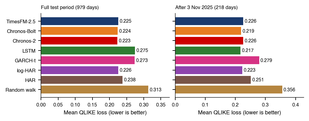
 MFM_ch14_acf_signal