Bucharest University of Economic Studies IDA Institute Digital Assets Blockchain Research Center AI4EFin Artificial Intelligence for Energy Finance Romanian Academy, Institute for Economic Forecasting MSCA Digital Finance
When Does One Bank's Distress Become the System's Problem?
“We propose a measure of systemic risk, \(\Delta\)CoVaR, defined as the change in the value at risk of the financial system conditional on an institution being under distress relative to its median state.” — Adrian & Brunnermeier (2016)
Thirteen banks from the US (United States), Europe and Romania, January 2010–September 2026
their declines are simultaneous: the euro-area crisis, COVID-19, the 2023 bank failures
Risk of each bank in isolation: VaR 1% (Value-at-Risk), the daily loss exceeded with probability 1%
contribution to the system: \(\Delta\)CoVaR 1% (CoVaR: the VaR of the system when an institution is in distress), the additional loss of the system when the bank moves from its median to its VaR
The two rankings hardly agree: the Spearman rank correlation between VaR and \(\Delta\)CoVaR is \(0.13\), across eleven banks
Deutsche Bank and ING (the Dutch ING Groep) have the largest VaR (\(7.19\%\) and \(7.16\%\)), but only an average \(\Delta\)CoVaR
JPMorgan has one of the smallest VaR (\(4.83\%\)), but one of the largest \(\Delta\)CoVaR
The systemic measures do not give a single ranking either
MES 5% (Marginal Expected Shortfall): the average loss of the bank on the worst 5% of market days
the rank correlation between MES 5% and \(\Delta\)CoVaR 1% is \(-0.04\)
We propose a measure of systemic risk, ΔCoVaR, defined as the change in the value at risk of the financial system conditional on an institution being under distress relative to its median state.
Systemic risk is the risk that the distress of one or more institutions affects the financial system as a whole and, through it, the real economy. It is an externality: a bank does not pay for the losses its failure imposes on others. The chapter uses daily prices of thirteen banks from the US (United States), Europe and Romania, from January 2010 to 18 September 2026. The declines of the three banking systems are simultaneous, in the euro-area crisis, the COVID-19 pandemic and the 2023 bank failures, and the maximum drawdown of the bank portfolio is 51% in the US, 61% in Europe and 47% in Romania.
The usual risk measure of a bank, Value-at-Risk (VaR), looks at the bank in isolation. Adrian & Brunnermeier (2016) measure instead its contribution to the system: ΔCoVaR 1% is the additional loss of the system when the bank moves from its median state to its own VaR. Across the eleven international banks, the Spearman rank correlation between VaR 1% and ΔCoVaR 1% is 0.13. Deutsche Bank and ING (ING Groep, Internationale Nederlanden Groep, the Dutch banking group ING) have the largest VaR, 7.19% and 7.16%, but only an average ΔCoVaR, while JPMorgan has one of the smallest VaR, 4.83%, but one of the largest ΔCoVaR. Regulating each bank by its own VaR therefore ignores its contribution to the system; with eleven banks and overlapping confidence intervals, however, the correlation remains very uncertain.
The systemic measures do not produce a single ranking either. The rank correlation between MES 5% (Marginal Expected Shortfall), the average loss of the bank on the worst 5% of market days, and ΔCoVaR 1% is −0.04, and the one between ΔCoVaR and the net volatility spillover is also −0.04; by contrast, VaR and MES have a rank correlation of 0.88. The chapter treats in turn the three families of measures, exposure (MES and SRISK), contribution (CoVaR) and connectedness (spillover networks and the Financial Risk Meter), and then stress tests and climate risk.
Systemic risk concerns the financial system rather than a single institution. The chapter asks when the distress of one bank becomes a problem for the system, and measures the answer in three ways:
The exposure of a bank to a market crash;
Its contribution to the tail loss of the system;
The network of links through which shocks travel.
The first section defines the concept, recalls two bank runs and the channels of contagion, and fixes the data and the sign conventions used throughout.
Systemic risk is the risk that the distress of one or several institutions impairs the financial system as a whole and, through it, the real economy. It is an externality: a bank does not pay for the losses that its failure imposes on others, so its private choice of capital and risk does not account for them. A measure of systemic risk must therefore look beyond the bank's own loss distribution.
Exposure asks what the bank loses when the market crashes; the Marginal Expected Shortfall (MES) gives its average loss on crash days and SRISK its capital shortfall in a crisis.
Contribution asks how much worse the system is when the bank is in distress; it is measured by ΔCoVaR, where CoVaR is the Value-at-Risk (VaR) of the system conditional on the bank.
Connectedness asks through which links shocks travel, and is measured with spillover and tail networks.
In brief
From one bank to the system
Systemic risk: the risk that the distress of one or several institutions impairs the financial system as a whole
and, through it, the real economy
An externality: a bank does not pay for the losses its failure imposes on others
Part I goes from the data to bank-level measures. After the data and conventions, it treats exposure through MES, LRMES (the MES of a crisis lasting months) and SRISK, and contribution through CoVaR and ΔCoVaR, with a discussion of how far the resulting rankings can be trusted.
Part II turns to networks, stress tests and a research case: spillover networks and the Financial Risk Meter, stress tests and climate risk, a case study on quantile connectedness and one pass of the discovery loop with artificial intelligence (AI). The reference textbooks are Franke, Härdle & Hafner (2019) and Härdle, Chen & Overbeck (2017); detailed examples are in Further Topics and derivations in the Appendix.
In brief
Two parts
Part I: from the data to bank-level measures of systemic risk
data and conventions
exposure: MES, LRMES (the MES of a crisis lasting months), SRISK
contribution: CoVaR, \(\Delta\)CoVaR, and how far rankings can be trusted
Part II: networks, stress tests and a research case
spillover networks and the Financial Risk Meter
stress tests and climate risk
a case study on quantile connectedness
one pass of the discovery loop with AI (artificial intelligence)
What you should be able to do
compute the MES, LRMES and SRISK of a bank and the break-even leverage \(\Lambda^*\)
derive \(\Delta\)CoVaR from the quantile regression and test the differences between banks
compute the connectedness table of a VAR (Vector AutoRegression) and interpret the net spillover network
interpret the Financial Risk Meter, stress tests and quantile connectedness
Further Topics and Appendix: reading for familiarity
Two bank runs show how the distress of one institution becomes a matter for the system. Northern Rock, a British mortgage lender, was hit in 2007 by the freeze in funding markets that followed the US subprime losses, and its depositors queued in the street to withdraw their savings.
The run on Silicon Valley Bank (SVB) in 2023 was digital. The FDIC (Federal Deposit Insurance Corporation) took the bank over on 10 March (FDIC, 2023), and two days later all depositors of SVB and Signature Bank were protected on systemic risk grounds (Federal Reserve Board, 2023). The authorities treated the failure of a mid-sized bank as a threat to the system, which is the situation the measures of the chapter try to quantify in advance.
The distress of one bank becomes systemic through three channels:
In a funding run, depositors and lenders withdraw from any bank that looks similar to the one in trouble, so the shock spreads through beliefs rather than balance sheets.
With common exposures and fire sales, banks that hold similar assets are hit together, and the forced selling of one bank lowers the prices for every holder.
Through counterparty links, one bank's liability is another bank's asset, so a default passes losses directly to its creditors.
Market-based measures, such as those of the chapter, see the combined effect of the three channels in stock prices, without separating them.
In brief
One bank's distress becomes systemic through three channels
Funding runs: depositors and lenders withdraw from any bank that looks similar
Common exposures and fire sales: forced selling lowers prices for every holder
Counterparty links: one bank's liability is another bank's asset, so a default passes losses to its creditors
Thirteen Banks, Three Markets: Prices and Log Returns
The data are daily prices of thirteen banks in three markets, from January 2010 to 18 September 2026, adjusted for dividends and splits:
Six US banks (JPMorgan, Bank of America, Citigroup, Goldman Sachs, Morgan Stanley and Wells Fargo) with the S&P 500 (Standard & Poor's) index;
Five European banks (Deutsche Bank, BNP Paribas, Santander, ING and HSBC) with the Euro Stoxx 50;
Two Romanian banks (Banca Transilvania and BRD-Groupe Société Générale) with the BET (Bucharest Exchange Trading, index) index of the Bucharest Stock Exchange (BVB).
The VIX (CBOE Volatility IndeX) index, the implied volatility of the S&P 500, completes the data.
The series are first aligned on 3,962 common trading dates, which gives 3,961 log returns in percent between consecutive common dates, \(r_t = 100(\ln P_t - \ln P_{t-1})\). A return can therefore span several sessions: 177 intervals cover more than one S&P 500 session, up to six. The alignment matters little for the measures, since on each region's own calendar MES 5% changes by at most 0.17 points and ΔCoVaR 1% by at most 0.32 points.
Two special cases are handled separately:
For the Romanian banks, days without trades are removed.
The historical stress scenarios for the international banks start in 2007.
In brief
Group
Banks (ticker, used in some charts)
Market index
US banks
JPMorgan (JPM), Bank of America (BAC), Citigroup (C), Goldman Sachs (GS), Morgan Stanley (MS), Wells Fargo (WFC)
S&P 500
European banks
Deutsche Bank (DBK), BNP Paribas (BNP), Santander (SAN), ING (INGA), HSBC (HSBA)
Euro Stoxx 50
Romanian banks
Banca Transilvania (TLV), BRD-Groupe Société Générale (BRD; “BRD-Groupe SG” in charts)
BET
Volatility
the VIX index (implied volatility of the S&P 500)
Daily prices, January 2010 to 18 September 2026, adjusted for dividends and splits
Aligned on 3 962 common trading dates first, then 3 961 log returns between consecutive common dates, \(r_t = 100(\ln P_t - \ln P_{t-1})\), in %
A return can span several sessions: 177 intervals cover more than one session of the S&P 500 (Standard & Poor's 500), up to 6
On each region's own calendar, MES 5% changes by at most 0.17 points and \(\Delta\)CoVaR 1% by at most 0.32 points
Special cases
Romanian banks, traded on the Bucharest Stock Exchange (BVB, index BET): days without trades removed
Historical stress scenarios for the international banks start in 2007
Losses as Positive Numbers and the System Portfolio
For a return \(X\) the loss is \(L = -X\), and the level \(\alpha\) is a tail probability, as in Chapter 7. The Value-at-Risk is
\[\mathrm{VaR}_\alpha(X) = -q_\alpha(X),\]
(18.1)
where \(q_\alpha\) is the \(\alpha\)-quantile of \(X\). The chapter writes VaR 1%, CoVaR 1% and MES 5%, all positive when they are losses.
The system return \(X^{sys}\) of a bank is the equal-weighted portfolio of the other banks of the same region, \(X^{sys} = \frac{1}{n}\sum_j X_j\). With log returns, this average is a first-order approximation of the log return of the daily rebalanced portfolio. CoVaR is stated for this aggregate, while MES conditions on the regional market index.
In brief
Return \(X\), loss \(L = -X\)
the level \(\alpha\) is a tail probability (Chapter 7)
\(\VaR_\alpha(X) = -q_\alpha(X)\), with \(q_\alpha\) the \(\alpha\)-quantile of \(X\)
We write VaR 1%, CoVaR 1%, MES 5%, all positive when they are losses
System return \(X^{sys}\): the equal-weighted portfolio of the other banks of the same region
\(X^{sys} = \frac{1}{n}\sum_j X_j\), a first-order approximation of the log return of the daily rebalanced portfolio
CoVaR is stated for this aggregate, while MES conditions on the regional market index
The chart plots, for each region, the equal-weighted portfolio of its banks, rebalanced daily, as a synthetic index of local-currency returns equal to 100 in January 2010, with vertical lines at the episodes used in the chapter. There is no currency conversion: HSBC is in pounds sterling and the other European banks in euros. The banks are those listed today, so the sample consists of survivors selected with hindsight.
Question for the room Which of the three bank portfolios had the largest drawdown since 2010, and when did it reach its trough?
Answer
The European portfolio: 61%, with the trough on 2020-04-21. The US portfolio lost 51% up to 2011-11-23 and the Romanian one 47% up to 2012-06-06. The annualised volatility of the bank portfolios is 29%, 30% and 23%, against 18%, 21% and 18% for the S&P 500, Euro Stoxx 50 and BET.
At the end of the sample the indices stand at 791 for the US, 384 for Europe and 1,233 for Romania. The maximum drawdown is 51% for the US portfolio (23 November 2011), 61% for the European one (21 April 2020) and 47% for the Romanian one (6 June 2012). The annualised volatility of the bank portfolios, 29%, 30% and 23%, exceeds that of the market indices, 18%, 21% and 18%.
The falls are simultaneous: the euro crisis, COVID-19 and the 2023 bank failures hit all three systems. The Romanian banks also have a shock of their own, the bank-tax announcement of December 2018, labelled "RO bank tax" in the chart.
In brief
Equal-weighted portfolios of the banks of each region, rebalanced daily
Vertical lines mark the episodes used in this chapter
No currency conversion: European banks in euro (EUR), HSBC (originally the Hongkong and Shanghai Banking Corporation) in pounds sterling (GBP)
Banks listed today: survivors selected with hindsight
Synthetic indices of local-currency returns (January 2010 = 100): 791 (US), 384 (Europe), 1 233 (Romania)
Maximum drawdown: US \(51\%\) (2011-11-23), Europe \(61\%\) (2020-04-21), Romania \(47\%\) (2012-06-06)
Systemic risk is an externality, and the chapter measures it in three ways: exposure, contribution and connectedness. The data are daily returns of thirteen banks in three regions, aligned on common dates, with losses reported as positive numbers and the system of a bank defined as the other banks of its region.
Exposure: MES and SRISK
Exposure measures what a bank loses when the market is in distress. The section starts from a single crash day (MES), extends the loss to a crisis lasting months (LRMES) and converts it into the capital the bank would lack after the crisis (SRISK), with the break-even leverage at which the shortfall appears.
How Much Does a Bank Lose When the Market Crashes?
The relevant loss for systemic risk is that of the bank given a market crisis, not its stand-alone VaR. What matters are the banks that run out of capital exactly when the system needs it, because their shortfalls arrive together and cannot be covered by other banks.
The section proceeds in three steps, from one crash day to a crisis:
The question: how much does a bank lose on average on the days when the market has a very bad day?
The computation: pick the worst 5% days of the market index (about 200 days out of 3 961) and average the bank's losses on those same days
Compare with the market: on these days the S&P 500 lost 2.72% on average, JPMorgan 3.21%, Morgan Stanley 4.03%
the banks lose more than the market precisely on the market's bad days
The difference from VaR: VaR looks at the bank's bad days; MES looks at the market's bad days, when the other banks suffer too
Why "marginal": if the market were itself a portfolio of these banks, its average loss on the bad days would split exactly across the banks by MES, weighted by their weights
our indices are not such portfolios, so here MES measures the bank's exposure
The next step, LRMES, goes from one bad day to a six-month crisis
Marginal Expected Shortfall and the Euler Property
the average loss of the bank on the worst \(\alpha\) share of days for the market \(m\). The name "marginal" comes from the Euler property: if \(m = \sum_i w_i X_i\) is the portfolio itself, then the Expected Shortfall of the portfolio decomposes as \(\mathrm{ES}_\alpha(X_m) = \sum_i w_i\,\mathrm{MES}_{i,\alpha}\). This is the Euler allocation, proved in the Appendix.
The market indices of the chapter are not portfolios of these 13 banks, so here MES measures exposure, not a share of the index ES (Expected Shortfall). The historical estimate averages \(-X_i\) over the days with \(X_m \le \hat q_\alpha(X_m)\); with \(\alpha = 5\%\) and 3,961 days, these are about 200 days.
\(\MES_{i,\alpha} = -\E\left[X_i \mid X_m \le q_\alpha(X_m)\right]\): the average loss of the bank on the worst \(\alpha\) share of days for the market \(m\)
Why “marginal”: if\(m = \sum_i w_i X_i\) is the portfolio itself, then \(\ES_\alpha(X_m) = \sum_i w_i\,\MES_{i,\alpha}\)
this is the Euler allocation (proof in the Appendix)
Our market indices are not portfolios of these 13 banks
Here MES measures exposure, not a share of the index ES (Expected Shortfall)
Historical estimate: average \(-X_i\) over the days with \(X_m \le \hat q_\alpha(X_m)\)
With \(\alpha = 5\%\) and 3 961 days, about 200 days
Question for the room If ▶ increases α from 5% to 10%, must MES fall for every bank?
Answer
There is no such guarantee. The added days are selected by the market return, not by the bank return, so the MES of a bank need not decrease in α. In this sample it falls for every bank: for JPMorgan, from 3.21% to 2.34%; this is an empirical result, not a general property. At α = 5%, the S&P 500 loses 2.72% on average on those days, and the US banks between 3.21% (JPMorgan) and 4.03% (Morgan Stanley); in Europe, HSBC loses 2.53%, against 3.16% for the Euro Stoxx 50.
The chart shows the MES 5% of each of the thirteen banks with its 95% bootstrap interval, together with the MES of the market indices themselves on the same days.
The bars give the average daily loss of each bank on the worst 5% of days for its market index, 2010–2026, with 95% intervals from a moving-block bootstrap with blocks of 20 days. MES exists if the bank's loss is integrable on the market's tail days. The Normal interval needs a finite long-run variance of the influence function and weak dependence, not in general a fourth moment.
The US banks range from 3.21% (JPMorgan) to 4.03% (Morgan Stanley), and in Europe MES reaches 4.79% (ING). On the same days the markets lose less, 2.72% for the S&P 500 and 3.16% for the Euro Stoxx 50, so the banks lose more than their market. HSBC is the exception in Europe, at 2.53%, below the index: it has a London listing with business concentrated in Asia. In Romania, Banca Transilvania has an MES of 3.14% and BRD 2.69%, the same as the BET index itself, 2.69%. The result supports a description of exposure.
In brief
Average daily loss of each bank on the worst 5% of days for its market index, 2010–2026
95% intervals: moving-block bootstrap, blocks of 20 days
MES exists if the bank's loss is integrable on the market's tail days
The Normal interval needs a finite long-run variance of the influence function and weak dependence, not in general a fourth moment
US banks: \(3.21\%\) (JPMorgan) to \(4.03\%\) (Morgan Stanley)
Europe up to \(4.79\%\) (ING)
Same days, market: \(2.72\%\) (S&P 500), \(3.16\%\) (Euro Stoxx 50): banks lose more
HSBC is the exception in Europe (\(2.53\%\), below the index)
A London listing with business concentrated in Asia
Banca Transilvania \(3.14\%\), BRD (BRD–Groupe Société Générale) \(2.69\%\)
BET itself \(2.69\%\)
Type of evidence: description (it shows what happened in the data, without testing a cause)
MES looks at a single bad day; a real crisis lasts months, for example a market fall of 40% in six months
LRMES: how much the bank's shares lose, on average, if the market goes through such a crisis
The simple version, without simulation: start from the bank's loss on a day when the market falls by more than 2% (\(\MES^{2\%}\)) and extend it to a long crisis
the factor 18 makes the step from one day to six months, with a constant beta: \(\mathrm{LRMES}\approx1-e^{-18\,\MES^{2\%}}\)
example: \(\MES^{2\%}=3\%\) gives 41.7%
For our banks: from 37% (HSBC) to 58% (ING); JPMorgan 48%, Banca Transilvania 52%
several banks would lose more than the market itself
The version in Further Topics: simulate many six-month paths and average the bank's loss over those in which the market falls by more than 40%
Why it matters: LRMES enters SRISK directly; the more the shares fall, the less capital remains
where \(R\) are the \(h\)-day arithmetic returns of the bank and the market. A crisis is a market fall below \(C = -40\%\) over six months (Acharya, Engle & Richardson, 2012), or below \(C = -10\%\) over \(h = 22\) days (Brownlees & Engle, 2017).
Acharya, Engle & Richardson (2012) give a shortcut without simulation, \(\mathrm{LRMES}_i \approx 1 - \exp(-18 \times \mathrm{MES}_i^{2\%})\), where \(\mathrm{MES}_i^{2\%}\) is the average daily loss of the bank on days when the market falls by more than 2%. The factor 18 scales the daily loss to the six-month crisis, under a constant beta. For example, \(\mathrm{MES}^{2\%} = 3\%\) gives \(1 - e^{-0.54} = 41.7\%\). On the chapter's banks the shortcut LRMES ranges from 37% (HSBC) to 58% (ING), with 48% for JPMorgan and 52% for Banca Transilvania.
In brief
LRMES (Long-Run MES): the expected fall of the bank's market equity in a crisis
\(\mathrm{LRMES}_{i,t} = -\E_t\left[R_{i,t+1:t+h} \mid R_{m,t+1:t+h} < C\right]\), with \(R\) the \(h\)-day arithmetic returns of bank and market
The question: if the market falls by 40% in six months, how much new money would the bank need to stay adequately capitalised?
Three ingredients: how much the bank owes (\(D\)), what its shares are worth today (\(W\)) and how much the shares would fall in the crisis (LRMES)
The computation on the chapter's example: \(D=900\), \(W=100\), LRMES \(=41.7\%\)
after the crisis, the shares are worth \((1-0.417)\times100=58.3\)
the prudential rule requires capital of at least \(k=8\%\) of quasi-assets: \(0.08\times(900+58.3)=76.7\)
\(76.7-58.3=18.4\) is missing: this is SRISK
A positive SRISK: a capital hole that, in a crisis, someone would have to fill (new shareholders or the state); the sum over banks is the SRISK of the system
What makes it large: large debt relative to capital and a large fall of the shares in the crisis
for our banks LRMES runs from 37% (HSBC) to 58% (ING)
SRISK is the capital a bank would lack in a severe market crisis (Brownlees & Engle, 2017). Equity must be at least a share \(k\) of quasi-assets, the book debt \(D\) plus the market equity \(W\). Assuming that debt is not renegotiated in the crisis,
which can be written \(k[D_i + (1-\mathrm{LRMES}_i)W_i] - (1-\mathrm{LRMES}_i)W_i\): the capital required after the crisis minus the capital left.
The prudential ratio is \(k = 8\%\) for US firms (Brownlees & Engle, 2017) and \(k = 5.5\%\) for European firms (Engle, Jondeau & Rockinger, 2015). The lower European ratio reflects accounting: IFRS (International Financial Reporting Standards) balance sheets allow less netting of derivatives than US GAAP (Generally Accepted Accounting Principles), so they report larger assets. A positive SRISK is a capital shortfall, and the system SRISK, the sum of the positive values, is published by the V-Lab of NYU (New York University) Stern.
In brief
SRISK (systemic risk): the capital a bank would lack in a severe market crisis
Equity must be at least a share \(k\) of quasi-assets, book debt \(D\) plus market equity \(W\)Brownlees & Engle (2017)
\(\mathrm{SRISK}_i = k\,D_i - (1 - k)(1 - \mathrm{LRMES}_i)\,W_i\), assuming debt is not renegotiated in the crisis
IFRS (International Financial Reporting Standards) balance sheets allow less netting of derivatives than US GAAP (Generally Accepted Accounting Principles)
In a numerical example with \(D = 900\),\(W = 100\), so \(\Lambda = 10\), and \(\mathrm{LRMES} = 41.7\%\),\(\mathrm{SRISK} = 0.08 \times 900 - 0.92 \times (1 - 41.7\%) \times 100 = 72 - 53.6 = 18.4\). Since \(\Lambda^* = 7.7 < \Lambda = 10\), the bank has a shortfall.
The chapter's data contain prices, not balance sheets. It therefore reports \(\Lambda^*\) from the estimated LRMES and treats leverage as an assumption.
Question for the room With k = 8%, from what leverage does ING need new capital in a 40% market crash? And with k = 5.5%?
Answer
From Λ* = 5.8 with k = 8% and from 8.2 with k = 5.5%. For HSBC, the bank with the lowest LRMES (37%), the thresholds are 8.3 and 11.9. A lower prudential ratio raises the threshold of every bank.
The chart plots SRISK per unit of market equity against an assumed leverage \(\Lambda\) for the banks with the highest, median and lowest LRMES; the dots mark the break-even leverage (18.5) of each bank.
The leverage on the horizontal axis is assumed, not observed. With \(k = 8\%\) and the shortcut LRMES, the curves in the chart have \(\Lambda^* = 5.8\) for ING, 6.4 for Santander and 8.3 for HSBC; for the other banks the threshold is 7.0 for JPMorgan, 6.0 for Morgan Stanley, 6.5 for Banca Transilvania and 7.1 for BRD. Above \(\Lambda^*\) the bank needs new capital in a 40% market crash, that is, with debt above 4.8–7.3 times market equity. With \(k = 5.5\%\) the thresholds rise, to 8.2 for ING and 11.9 for HSBC, so SRISK depends on the chosen prudential ratio.
The calculation has limits. LRMES extrapolates daily data, and market equity itself falls in a crisis. The LRMES simulated with GJR (Glosten–Jagannathan–Runkle, asymmetric GARCH)–GARCH (Generalised AutoRegressive Conditional Heteroskedasticity) and DCC (Dynamic Conditional Correlation) is 0.43 to 0.92 times the shortcut value (Further Topics), so \(\Lambda^*\) depends on the model. The result supports a description: a threshold computed for an assumed leverage, not an observed capital shortfall.
In brief
Banks with the highest, median and lowest LRMES
dots mark \(\Lambda^*\)
Leverage on the horizontal axis is assumed, not observed
Curves in the chart, with \(k = 8\%\) and the shortcut LRMES: \(\Lambda^* = 5.8\) (ING), \(6.4\) (Santander), \(8.3\) (HSBC)
Other banks: JPMorgan \(7.0\), Morgan Stanley \(6.0\), Banca Transilvania \(6.5\), BRD \(7.1\)
Above \(\Lambda^*\) the bank needs new capital in a 40% market crash
i.e. with debt above \(4.8\)–\(7.3\) times market equity
With \(k = 5.5\%\) the thresholds rise (ING \(8.2\), HSBC \(11.9\))
SRISK depends on the chosen prudential ratio
Limits of the calculation
LRMES extrapolates daily data
market equity itself falls in a crisis
LRMES simulated with an asymmetric GARCH (GJR) and dynamic conditional correlations (DCC) is 0.43 to 0.92 of the shortcut (Further Topics): \(\Lambda^*\) depends on the model
Type of evidence: description
a threshold computed for an assumed leverage, not an observed capital shortfall
MES measures the bank's loss on market crash days; on the chapter's data most banks lose more than their index. LRMES extends the loss to a six-month crisis, and SRISK turns it into a capital shortfall, which without balance sheets is summarised by the break-even leverage. The thresholds depend on the prudential ratio and on the model for LRMES.
Contribution: CoVaR
Contribution reverses the direction of exposure: it asks how much worse the tail of the system becomes when a given bank is in distress. The section defines CoVaR and ΔCoVaR, estimates them by quantile regression, tests whether the contributions differ between banks and compares them with the bank's own VaR and with its exposure. It ends with the question of how far rankings of banks by these measures can be trusted.
How Much Worse Is the System When a Bank Is in Distress?
MES looks from the market to the bank; contribution looks the other way, from the bank to the system. The object of interest is a quantile in the tail of the system's return, not its mean, so the natural tool is quantile regression, which estimates the conditional quantile directly (Koenker & Bassett, 1978).
The levels are \(\alpha = 1\%\) and \(\alpha = 5\%\), those reported by Adrian & Brunnermeier (2016), and the rankings at the two levels are compared. The section asks how much each bank adds to the tail loss of the system and whether the differences between banks are statistically significant.
In brief
MES looks from the market to the bank
contribution looks the other way, from the bank to the system
We need a quantile in the tail of the system, not its mean
The VaR of a bank answers the question: how much can the bank lose on one of its worst 1% days?
The regulator has another question: how much does the rest of the banking system lose on a day when this bank is in distress?
CoVaR: the VaR of the system, computed for the days on which the bank is at its own VaR
\(\Delta\)CoVaR: how much this loss of the system rises compared with an ordinary day for the bank (median return)
it is the bank's contribution to the tail risk of the system, not its own risk
The two can differ a lot: a bank with small losses of its own can drag the system down with it
JPMorgan has one of the smallest VaR (4.83%), but one of the largest \(\Delta\)CoVaR
Deutsche Bank has the largest VaR (7.19%), but only an average \(\Delta\)CoVaR
The estimation in words: draw the line that follows the worst 1% days of the system as a function of the bank's return (quantile regression); its slope shows how much the bank adds
CoVaR: the VaR of the System Given a Bank in Distress
with the bank return fixed at the quantile shown. ΔCoVaR measures the contribution of bank \(i\) to the tail risk of the system. Reversing the roles of bank and system gives the exposure CoVaR, the VaR of bank \(i\) when the system is in distress.
The loss of the system that is exceeded with probability \(\alpha\) on a day when bank \(i\) is at its own VaR
\(\Delta\)CoVaR: the change from the median state of the bank, a normal day, to its distress state
\(\Delta\CoVaR_\alpha^{sys|i} = \CoVaR_\alpha^{sys|X_i = q_\alpha} - \CoVaR_\alpha^{sys|X_i = q_{50\%}}\), with the bank return fixed at the quantile shown
\(\Delta\)CoVaR measures the contribution of bank \(i\) to the tail risk of the system
Reversing the roles gives the exposure CoVaR
the VaR of bank \(i\) when the system is in distress
Uncertainty is measured by a moving-block bootstrap with 999 resamples, which keeps volatility clustering. The block length grows like \(n^{1/3}\)(Hall, Horowitz & Jing, 1995):\(3{,}961^{1/3} \approx 16\), rounded to 20 observations, about one trading month.
Question for the room With α fixed at 1%, what happens to the 1% quantile regression line when ▶ increases the number of displayed days?
Answer
It stays the same: the coefficients are estimated on the full sample and stay fixed; ▶ only changes the visible points and the share of them below the line. The animation is not a recursive estimation. CoVaR 1% is 6.64% with JPMorgan at its VaR 1% (4.83%), against 2.03% with JPMorgan at its median; the difference, ΔCoVaR 1% = 4.62%, is the slope 0.94 times the distance between the two JPMorgan quantiles. The unconditional system VaR 1% is 5.07%.
The chart shows the daily returns of the other US banks against those of JPMorgan, 2010–2026, with the 1% and 50% quantile regression lines and a dotted line at JPMorgan's VaR 1%.
The fitted 1% line is \(\hat q_{1\%} = -2.10 + 0.94\,X_i\) and the median line \(-0.03 + 0.96\,X_i\). The slopes are similar, so the 1% line is shifted down, not steeper.
With JPMorgan at its VaR 1%, 4.83%, the CoVaR 1% of the other US banks is 6.64%, against a system VaR 1% of 5.07% and a CoVaR 1% of 2.03% with JPMorgan at its median. By (18.9),\(\Delta\mathrm{CoVaR}_{1\%} = 4.62\%\): JPMorgan in distress adds about 4.62 points to the tail loss of the system. This is an association, not a causal effect, because a common shock hits all banks on the same day.
In brief
Daily returns 2010–2026, 1% and 50% quantile regression lines
dotted line: JPMorgan at its VaR 1%
1% line: \(\hat q_{1\%} = -2.10 + 0.94\,X_i\)
median line: \(-0.03 + 0.96\,X_i\)
Similar slopes: the 1% line is shifted down, not steeper
With JPMorgan at its VaR 1% (\(4.83\%\)), the other US banks have CoVaR 1% \(= 6.64\%\)
Against the system VaR 1% of \(5.07\%\) and the CoVaR 1% of \(2.03\%\) with JPMorgan at its median
\(\Delta\CoVaR_{1\%} = 4.62\%\)
JPMorgan in distress adds about \(4.62\) points to the tail loss of the system
Association, not causation: a common shock hits all banks on the same day
Question for the room Is Wells Fargo, with the largest ΔCoVaR 1%, significantly more systemic than Citigroup, with the smallest?
Answer
The estimates are 4.89% and 3.81%, but none of the 25 within-region pairs differs after the Holm correction. The overlap of the intervals [3.27, 4.79] and [3.68, 5.73] is not the test. The joint Wald test rejects equal contributions of the US banks (p = 0.011). At α = 5% the ranking changes: its Spearman correlation with the 1% ranking is 0.13.
The chart shows the ΔCoVaR 1% of the eleven international banks with 95% bootstrap intervals.
The bars give ΔCoVaR, the extra system loss when the bank moves from its median to its VaR, with 95% bootstrap intervals. The Romanian banks are left out: with only two, the "system" of the other bank would be a single bank. The estimates range from 3.81% (Citigroup) to 4.89% (Wells Fargo), with intervals 1.5–2.8 points wide.
The marginal intervals overlap, for example Citigroup [3.27, 4.79] and Wells Fargo [3.68, 5.73]. Overlap is not a test: estimates from the same days are strongly correlated, so the interval for the difference can be narrower; the tests follow on the next slide.
At \(\alpha = 5\%\) the values are smaller (2.63% for JPMorgan) and the ranking changes. The Spearman correlation between the rankings at 1% and 5% is 0.13, a fragile basis for regulation. The result supports an association.
In brief
Bars: \(\Delta\)CoVaR, the extra system loss when the bank moves from its median to its VaR
with 95% bootstrap intervals
No Romanian banks: with only two, the “system” of the other bank would be one single bank
From \(3.81\%\) (Citigroup) to \(4.89\%\) (Wells Fargo)
intervals 1.5–2.8 points wide
The marginal intervals overlap, e.g. Citigroup \([3.27, 4.79]\) and Wells Fargo \([3.68, 5.73]\)
Overlap is not a test
estimates from the same days are strongly correlated
so the interval for the difference can be narrower
At \(\alpha = 5\%\) the values are smaller (JPMorgan \(2.63\%\)) and the ranking changes
Spearman correlation of the 1% and 5% rankings: also \(0.13\) (by coincidence, as for VaR vs \(\Delta\)CoVaR), a fragile basis for regulation
Type of evidence: association (the variables move together; this does not prove causation)
All tests use the same 999 block-bootstrap draws for every bank, so the estimates keep their dependence (details in the Appendix). Three hypotheses are tested:
No contribution, \(H_0: b_\alpha = 0\), tested with the standard error of the slope \(\hat b_{1\%}\) from the bootstrap draws and a Holm (1979) correction over the 11 banks. The \(z\)-ratios range from 8.7 (HSBC) to 22.6 (Citigroup), so the slope is positive for all 11 banks, also after Holm. With the kernel sandwich standard error of Hendricks & Koenker (1992), valid only for serially uncorrelated scores, the \(t\)-ratios are between 4.0 and 6.9.
Equal tail and median slopes, \(H_0: b_\alpha = b_{50\%}\): the test asks whether the tail slope differs from the median slope. It is rejected for 2 of the 11 banks, Citigroup and ING, also after Holm; not rejecting for the other 9 does not prove equality.
Equal contributions, \(H_0: \Delta\mathrm{CoVaR}_i = \Delta\mathrm{CoVaR}_j\); dominance tests are in Castro & Ferrari (2014) and the results by bank in the Appendix. At \(\alpha = 1\%\), 4 of the 25 within-region pairs differ at 5%, none after Holm, and the joint Wald test gives \(p = 0.011\) for the US and \(p = 0.28\) for Europe. At \(\alpha = 5\%\), 3 of 25 pairs differ, none after Holm, with joint Wald \(p = 0.017\) for the US and \(0.038\) for Europe.
In brief
All tests use the same 999 block-bootstrap draws for every bank
so the estimates keep their dependence (details: Appendix)
(1) No contribution, \(H_0\colon b_\alpha = 0\)
Standard error of the slope \(\hat b_{1\%}\) from the same bootstrap draws, Holm (1979) correction over the 11 banks
\(z\)-ratios from \(8.7\) (HSBC) to \(22.6\) (Citigroup): the slope is positive for all 11 banks, also after Holm (Quantile Regression: Asymptotics)
With the kernel sandwich standard error Hendricks & Koenker (1992), valid only for serially uncorrelated scores: \(t\) from \(4.0\) to \(6.9\)
(2) Tail slope equal to the median slope, \(H_0\colon b_\alpha = b_{50\%}\): rejected for 2 of 11 banks (Citigroup, ING, also after Holm)
not rejecting for the other 9 does not prove equality
With 25 pairs tested at 5%, more than one false "difference" is expected even if all contributions are equal, so the pairs are treated as one family. The procedure of Holm (1979) sorts the p-values, \(p_{(1)} \le \dots \le p_{(m)}\), and rejects while \(p_{(k)} \le 0.05/(m-k+1)\); the family-wise error stays below 5% for any dependence between the tests. In a toy check with \(p = 0.010, 0.030, 0.040\), the first is rejected because \(0.010 \le 0.05/3\), and the procedure stops at the second because \(0.030 > 0.05/2\): one rejection instead of three.
The joint Wald test of equal contributions within a region uses \(W = \hat d^\top \hat V^{-1} \hat d\), which is \(\chi^2\) with the number of banks minus one degrees of freedom; \(\hat d\) collects the differences from one reference bank, any choice giving the same \(W\), and \(\hat V\) is their bootstrap covariance.
For the US, the joint test rejects (\(p = 0.011\)) while none of the 25 pairs survives Holm. The two results are compatible: the joint test pools moderate differences, while Holm needs one very strong pair, \(p_{(1)} \le 0.05/25\). The contributions are therefore not all equal, but the data do not say which pair differs.
In brief
Many pairs, one family: 25 pairs tested at 5%
more than one false “difference” is expected even with equal contributions
Holm (1979): sort \(p_{(1)} \le \dots \le p_{(m)}\) and reject while \(p_{(k)} \le 0.05/(m - k + 1)\)
The family-wise error stays below 5% for any dependence
Toy check, \(p = 0.010, 0.030, 0.040\): \(0.010 \le 0.05/3\) (reject), \(0.030 > 0.05/2\) (stop): one rejection instead of three
Joint Wald test of equal contributions within a region
\(W = \hat d^\top \hat V^{-1} \hat d \sim \chi^2\) with the number of banks minus 1 degrees of freedom
\(\hat d\): differences from one reference bank (any choice gives the same \(W\))
\(\hat V\): their bootstrap covariance
US: the joint test rejects (\(p = 0.011\)) while 0 of 25 pairs survive Holm
The joint test pools moderate differences; Holm needs one very strong pair (\(p_{(1)} \le 0.05/25\))
So the contributions are not all equal, but we do not know which pair differs
Question for the room At α = 1%, the Spearman correlation between VaR and ΔCoVaR is 0.13 across the 11 banks. What can we infer?
Answer
The estimated rank association is weak, without establishing independence. Spearman correlation describes rank association, not independence or a causal effect; 0.13 comes from only 11 banks and is uncertain. At α = 5% the estimate is −0.51: the tail level matters. Deutsche Bank and ING have the largest VaR 1% (7.19% and 7.16%) and only an average ΔCoVaR; JPMorgan has one of the smallest VaR (4.83%) and one of the largest ΔCoVaR (4.62%).
The chart plots, for the eleven banks, the VaR 1% of each bank on the horizontal axis against its ΔCoVaR 1% on the vertical axis, 2010–2026.
The Spearman rank correlation between VaR and ΔCoVaR is 0.13. Deutsche Bank and ING have the largest VaR, 7.19% and 7.16%, but only an average ΔCoVaR, while JPMorgan has one of the smallest VaR, 4.83%, and one of the largest ΔCoVaR.
This is the central message of Adrian & Brunnermeier (2016): regulating each bank by its own VaR ignores its contribution to the system. With eleven banks and overlapping intervals, however, the correlation itself is very uncertain, so the evidence is of a weak rank association, not of independence.
In brief
Horizontal axis: VaR 1% of the bank, vertical axis: its \(\Delta\)CoVaR 1%
eleven banks, 2010–2026
Spearman rank correlation between VaR and \(\Delta\)CoVaR: \(0.13\)
Deutsche Bank and ING: the largest VaR (\(7.19\%\), \(7.16\%\)), only average \(\Delta\)CoVaR
JPMorgan: one of the smallest VaR (\(4.83\%\)), one of the largest \(\Delta\)CoVaR
Question for the room At α = 1%, can we obtain the exposure of ING by inverting the coefficient of the quantile regression used for its contribution?
Answer
No. Reversing the conditioning requires a separate quantile regression, of the ING return on the system. For ING, the contribution is 4.41% and the exposure 6.14%, both measured against the median state of the conditioning variable; they describe associations in two directions, not causal effects. HSBC is the opposite case: contribution 4.07%, exposure 3.17%. Exposure exceeds contribution for four of the five European banks.
The chart compares, bank by bank, the contribution (blue), the loss of the system when the bank is in distress, with the exposure (orange), the loss of the bank when the system is in distress.
The exposure CoVaR is estimated by regressing \(X_i\) on \(X^{sys}\) and plugging in the quantiles of \(X^{sys}\); it is a separate regression, not a transformation of the contribution regression. The direction matters: ING has a contribution of 4.41% and an exposure of 6.14%, BNP Paribas 4.83% and 6.07%, while HSBC has a contribution of 4.07% and an exposure of only 3.17%. Exposure exceeds contribution for most European banks.
Both quantities are associations, not causal effects. Exposure matters for the bank's own capital, contribution for the regulator.
In brief
Blue, contribution: loss of the system when the bank is in distress
Orange, exposure: loss of the bank when the system is in distress
\(X_i\) regressed on \(X^{sys}\), quantiles of \(X^{sys}\) plugged in
The direction matters: ING has contribution \(4.41\%\) and exposure \(6.14\%\)
BNP Paribas (BNP: Banque Nationale de Paris): \(4.83\%\) and \(6.07\%\)
HSBC: contribution \(4.07\%\), exposure only \(3.17\%\)
Exposure exceeds contribution for most European banks
Rankings by different systemic measures disagree and carry wide uncertainty (Nucera, Schwaab, Koopman & Lucas, 2016), so measures should be combined and rank uncertainty reported. Model risk adds to this (Danielsson, James, Valenzuela & Zer, 2016): simulated against shortcut LRMES, Girardi–Ergün against quantile-regression CoVaR, and \(\alpha = 1\%\) against \(5\%\) can each change the order.
The effective tail sample \(\alpha n\) is 40 days at 1% and 198 at 5%. At 1% the kernel and block-bootstrap standard errors disagree (Appendix), and out-of-sample backtests of \(\mathrm{CoVaR}^{\le}_{5\%}\) reject for no bank (Appendix), but with about 7.4 expected joint hits their power is low.
What survives are large, tested differences, across regions and in the tail slope of some banks, not the order of eleven close point estimates.
Effective tail sample \(\alpha n\): \(40\) days at 1%, \(198\) at 5%
At 1% the kernel and block-bootstrap standard errors disagree (Appendix)
Out-of-sample backtests of the Girardi–Ergün CoVaR 5% reject for no bank (Appendix)
With about 7.4 expected joint hits their power is low
What survives are large, tested differences
across regions and in the tail slope of some banks
not the order of eleven close point estimates
Section summary
ΔCoVaR measures how much the tail loss of the system rises when a bank moves from its median to its VaR. All eleven banks contribute significantly, but pairwise differences do not survive the Holm correction, the ranking changes between 1% and 5%, and contribution is only weakly related to the bank's own VaR and differs from its exposure.
Connectedness: Spillover Networks
MES and CoVaR relate one bank to one aggregate, while a crisis travels between many banks at once. The section builds a network from the forecast-error variance decomposition of a vector autoregression on the banks' daily volatilities, reads the connectedness table and the net spillover network, and follows total connectedness over time.
Through Which Links Do Shocks Travel between Banks?
A network answers three questions that the bank-level measures leave open:
Who transmits shocks and who receives them;
How connected the system is as a whole;
Whether connectedness rises in crises.
The approach of the section is the forecast-error variance decomposition of a vector autoregression (VAR) (Diebold & Yilmaz, 2014), applied to the daily volatilities of the banks. The edges of the network are shares of forecast error variance, which can be estimated from prices alone.
In brief
MES and CoVaR look at one bank and one aggregate
a crisis, however, travels between many banks at once
A network looks at all pairs of banks at once. Its nodes are the banks, and a directed edge measures how much of the future uncertainty of bank \(i\) comes from shocks to bank \(j\). The model is a VAR of order \(p\) for \(N\) series \(y_t\),
in which each series is regressed on \(p\) lags of all series; \(c\) is the vector of constants, \(A_l\) are \(N \times N\) coefficient matrices, \(\varepsilon_t\) the shocks and \(\Sigma\) their covariance matrix (assumptions in the Appendix).
The \(H\)-day forecast error of \(y_i\) is a sum of shocks to all series, so its variance can be split by source. In the moving-average form \(y_t = \mu + \sum_{h\ge0}\Phi_h\,\varepsilon_{t-h}\),\(\Phi_h\) is the response of \(y\) after \(h\) days to a shock today, with \(\Phi_0 = I\). Orthogonal (Cholesky) shocks depend on the ordering of the series; the generalized decomposition of Koop, Pesaran & Potter (1996) and Pesaran & Shin (1998) does not.
The generalized share of the forecast error variance of \(i\) due to \(j\) is
where the numerator is the part of the forecast error variance of \(i\) due to a shock in \(j\), the denominator the total forecast error variance of \(i\),\(e_i\) the \(i\)-th unit vector and \(\sigma_{jj}\) the variance of shock \(j\), the \(j\)-th diagonal element of \(\Sigma\).
In brief
The \(H\)-day forecast error of \(y_i\) is a sum of shocks to all series
so its variance can be split by source
Moving-average form \(y_t = \mu + \sum_{h \ge 0}\Phi_h\,\varepsilon_{t-h}\): \(\Phi_h\) is the response of \(y\) after \(h\) days to a shock today, \(\Phi_0 = I\)
Orthogonal (Cholesky) shocks depend on the ordering of the series
In the connectedness table of Diebold & Yilmaz (2014),\(\tilde\theta_{ij}\) in percent is the share of the \(H\)-day forecast error variance of \(i\) due to shocks in \(j\). Each row sums to 100 after the normalisation in (18.11); before it, the rows do not, because generalized shocks are correlated.
The table yields four kinds of summary:
The spillover from others to \(i\) is \(F_i = \sum_{j\ne i}\tilde\theta_{ij}\) and the spillover to others from \(j\) is \(T_j = \sum_{i\ne j}\tilde\theta_{ij}\).
The net spillover \(T_i - F_i\) is positive for a net transmitter.
The pairwise net spillover \(\tilde\theta_{ji} - \tilde\theta_{ij} > 0\) means that \(i\) transmits net to \(j\), drawn as an arrow \(i \to j\).
annualised as \(100\sqrt{252\,\hat\sigma_t^2}\) and used in logs. The estimator is unbiased for the variance of a Brownian motion without drift and more efficient than the squared return. On 8 days the high equals the low although volume is positive (3 for Banca Transilvania, 5 for BRD); these are imputed with the smallest positive variance so far, not estimated by Parkinson's formula. Without these days total connectedness is 63.94%, against 63.93%.
The model is a VAR on the log volatility of the 13 banks, a range-based volatility as in Demirer et al. (2018). Volatility rather than returns is used because it jumps in crises, so its network shows where stress travels. The order chosen by the Bayesian information criterion (BIC) is \(p = 2\), and the horizon is \(H = 10\) days, as in Diebold & Yilmaz (2012). US banks close after European ones, and the VAR lags capture the transmission to the next day.
In brief
Parkinson volatility from the daily high price \(P^{\max}_t\) and low price \(P^{\min}_t\)Parkinson (1980)
\(\hat\sigma_t^2 = \dfrac{(\ln P^{\max}_t - \ln P^{\min}_t)^2}{4\ln 2}\), annualised \(100\sqrt{252\,\hat\sigma_t^2}\), used in logs
Unbiased for the variance of a Brownian motion without drift and more efficient than the squared return
8 days with high equal to low, all with positive volume (Banca Transilvania 3, BRD 5): imputed with the smallest positive variance so far, not Parkinson estimates
Without these days total connectedness is \(63.94\%\), against \(63.93\%\)
Our model: VAR on the log volatility of the 13 banks, a range-based volatility as in Demirer et al. (2018)
Volatility, not returns: it jumps in crises, so its network shows where stress travels
Order by the Bayesian information criterion (BIC): \(p = 2\)
Question for the room At H = 10, a US bank receives on average 84.0% of the forecast error variance of its volatility from US shocks, and the average own-shock share is 26.3%. How much comes, on average, from the other US banks?
Answer
About 57.8% = 84.0 − 26.3: we subtract the own shocks. 84.0% includes the own shocks; 73.7% = 100 − 26.3 includes all the other banks, from every region. The figures are averages over the six US banks. A US bank receives 15.0% from Europe; a European bank receives 72.7% from Europe and 26.2% from the US. Total connectedness, 63.9%, is the average over all banks of the share coming from the other banks. These are normalised shares computed from a VAR(2); residual autocorrelation limits their interpretation as shares of the forecast error variance.
The chart is the connectedness table of the thirteen banks over the full sample: row \(i\), column \(j\) gives the share in percent of the 10-day forecast error variance of bank \(i\) due to shocks in bank \(j\), with the banks labelled by the tickers of the data table.
Total connectedness (18.12) is \(C = 63.9\%\): on average, two thirds of a bank's volatility risk comes from the other banks. On returns instead of volatility, \(C = 75.4\%\).
The table has two regional blocks. A US bank receives 84.0% of its forecast error variance from US shocks and a European bank 72.7% from European shocks. Across the Atlantic, the share from US banks to a European bank is 26.2%, and 15.0% in the other direction. The Romanian banks are driven mostly by their own shocks, 72.3% for Banca Transilvania and 76.1% for BRD, with 10.3% from US banks and 8.0% from European banks.
The result supports a description: an edge is a share of forecast error variance, not a causal exposure. The VAR(2) residuals remain serially correlated (Appendix); with 22 lags, \(C = 59.6\%\).
In brief
Row \(i\), column \(j\): share (%) of the 10-day forecast error variance of bank \(i\) due to shocks in bank \(j\)
full sample (tickers of the data table)
Total connectedness \(C = 63.9\%\)
on average two thirds of a bank's volatility risk comes from the other banks
On returns instead of volatility: \(C = 75.4\%\)
Two regional blocks
a US bank receives \(84.0\%\) from US shocks
a European bank \(72.7\%\) from European shocks
Across the Atlantic: \(26.2\%\) from US to a European bank, \(15.0\%\) the other way
Romanian banks: mostly their own shocks
\(72.3\%\) (Banca Transilvania) and \(76.1\%\) (BRD)
From US banks \(10.3\%\), from European banks \(8.0\%\)
Type of evidence: description
an edge is a share of forecast error variance, not a causal exposure
The VAR(2) residuals remain serially correlated (Appendix); with 22 lags, \(C = 59.6\%\)
Question for the room With H fixed at 10, what happens to the net positions of the banks if we keep only the largest 5% of the positive pairwise net spillovers, instead of 25%?
Answer
They stay unchanged: net positions are computed from the full matrix, and the threshold only filters the drawing (4 arrows above 3.04 points, instead of 20 above 1.57). Fewer visible arrows do not mean lower estimated connectedness. Transmitters: Citigroup (+19.0), Bank of America (+10.9), Morgan Stanley (+9.9) and JPMorgan (+9.8). Receivers: HSBC (−23.6), BRD (−13.0), Deutsche Bank (−12.6) and Banca Transilvania (−12.2).
The chart draws the net spillover network: an arrow \(j \to i\) when \(j\) transmits net to \(i\), for the largest 25% of the pairwise net spillovers, with node size growing with the spillover to others.
The largest net transmitters are US banks: Citigroup (+19.0 points), Bank of America (+10.9), Morgan Stanley (+9.9) and JPMorgan (+9.8). The largest net receivers are HSBC (−23.6), BRD (−13.0), Deutsche Bank (−12.6) and Banca Transilvania (−12.2). HSBC receives from almost every bank: it trades in London, between Asia and New York. Within Europe, BNP Paribas and ING transmit to Deutsche Bank and Santander.
The network must be read with its uncertainty. Only 8 of the 13 net positions have marginal 95% bootstrap intervals that exclude zero (Further Topics), and a full-sample network averages quiet and crisis years.
In brief
Arrow \(j \to i\) when \(j\) transmits net to \(i\) (largest 25% of pairwise net spillovers)
Node size grows with the spillover to others
Net transmitters: Citigroup (\(+19.0\)), Bank of America (\(+10.9\)), Morgan Stanley (\(+9.9\)), JPMorgan (\(+9.8\))
Net receivers: HSBC (\(-23.6\)), BRD (\(-13.0\)), Deutsche Bank (\(-12.6\)), Banca Transilvania (\(-12.2\))
HSBC receives from almost every bank: it trades in London, between Asia and New York
Within Europe, BNP Paribas and ING transmit to Deutsche Bank and Santander
Only 8 of the 13 net positions have marginal 95% bootstrap intervals that exclude zero (Further Topics)
A full-sample network averages quiet and crisis years
Question for the room We keep H = 10 and shorten the rolling window from 250 to 100 trading days. How does the mechanical memory of the COVID-19 episode in the total connectedness index change?
Answer
The crisis observations leave the window sooner: each observation stays in the estimation window for fewer days. This can speed up the fall of the index without showing an economic change in transmission. With 250 days, the index rises from 61.8% on average in 2019 to 78.4% in spring 2020, with a maximum of 79.3% on 2020-08-27. With 100 days, the maximum is 85.6% on 2020-03-12, and the index first falls more than 10 points below it on 2020-08-13 (73.4%). There is no general rule for the size of the maximum.
The top panel of the chart shows total connectedness on rolling 250-day windows, with a VAR(2) and \(H = 10\) re-estimated every 5 days; the bottom panel shows the net spillover summed by region.
Total connectedness ranges from 47.4% (24 July 2024) to 79.3% (27 August 2020), with a mean of 62.0%. It rose from 61.8% in 2019 to 78.4% in the spring of 2020, with COVID-19; it was 66.0% after the 2023 bank failures and 53.5% in the calm year 2024. The index rises within days of a shock, while its fall about 250 days later partly reflects the crisis leaving the window. The levels depend on the window, the estimator and the VAR order, while the changes over time do not, as the elastic-net estimates in Further Topics show.
By region, the US banks are net transmitters in 89% of the windows, with a sum of net spillovers of +48.4 points on average. The European banks were net transmitters during the euro crisis of 2011–2012 and mostly net receivers afterwards, and the Romanian banks are net receivers, at −24.1 points on average.
In brief
Top: total connectedness on rolling 250-day windows
VAR(2), \(H = 10\), every 5 days
Bottom: net spillover summed by region
The total index ranges from \(47.4\%\) (2024-07-24) to \(79.3\%\) (2020-08-27)
mean \(62.0\%\)
COVID-19: from \(61.8\%\) in 2019 to \(78.4\%\) in spring 2020
After the 2023 bank failures \(66.0\%\), in the calm year 2024 \(53.5\%\)
The index rises within days
Its fall about 250 days later partly reflects the crisis leaving the window
Levels depend on the window, estimator and VAR order, the changes over time do not (elastic net, Further Topics)
US banks are net transmitters in \(89\%\) of the windows
sum of their net spillovers, on average \(+48.4\) points
European banks were net transmitters during the euro crisis of 2011–2012
and mostly net receivers afterwards
Romanian banks are net receivers on average (\(-24.1\) points on average)
The variance-decomposition network shows a system in which about two thirds of a bank's volatility risk comes from other banks, organised in regional blocks, with US banks as the main net transmitters and HSBC and the Romanian banks as net receivers. Connectedness rises quickly in crises, but the edges are forecast-variance shares, not causal exposures, and several net positions are not significantly different from zero.
Tail Networks: the Financial Risk Meter
The spillover network of the previous section describes how an average shock spreads, while systemic risk sits in the tail of the return distribution. This section moves the network into the tail with quantile regressions, as in the Financial Risk Meter, and asks whether the resulting indicator tracks systemic stress on the chapter's thirteen banks.
How Tight Are the Links between Banks in the Tail?
The Financial Risk Meter (FRM) of Mihoci, Althof, Chen & Härdle (2020) runs, for each firm \(j\), one quantile regression at \(\tau = 5\%\) of its return on the returns of all other firms and on lagged macro variables. With 100 firms and a window of 63 days there are more regressors than days, so the estimation needs a penalty. The LASSO (Least Absolute Shrinkage and Selection Operator) penalty keeps only the strong links, and the FRM is the average of the selected penalties, read as an indicator of tail interdependence and of systemic stress.
The question of the section is whether this indicator also tracks systemic stress on the 13 banks of the chapter. The panel is far smaller than the one for which the FRM was built, which matters for how the penalty behaves.
In brief
The spillover network describes an average shock, while systemic risk sits in the tail
over the \(n\) days of the window, where \(X_{j,t}\) is the return of firm \(j\),\(Z_{-j,t}\) collects the returns of the other firms and the lagged macro variables (the S&P 500 and Euro Stoxx 50 returns and the log change of the VIX), and \(\rho_\tau\) is the check loss of quantile regression. A larger \(\lambda\) leaves fewer active coefficients.
The penalty is chosen by GACV (Generalized Approximate Cross-Validation), which trades fit against the number of active coefficients:
where \(\hat X_{j,t}(\lambda)\) is the fitted quantile and \(\mathrm{df}(\lambda)\) the number of interpolated observations, equal to one plus the number of nonzero slopes. The selected \(\lambda_j\) minimises (18.15) for each firm, and the FRM is the average of the \(\lambda_j\) across firms.
\(\hat\beta_j(\lambda) = \arg\min_{\beta} \dfrac{1}{n}\sum_t \rho_\tau\left(X_{j,t} - \beta_0 - \beta^\top Z_{-j,t}\right) + \lambda\|\beta\|_1\), over the \(n\) days of the window
\(X_{j,t}\): return of firm \(j\)
\(Z_{-j,t}\): returns of the other firms and the lagged macro variables (S&P 500 and Euro Stoxx 50 returns, log change of the VIX)
A larger \(\lambda\) leaves fewer active coefficients
GACV (Generalized Approximate Cross-Validation) trades fit against the number of active coefficients
\(\mathrm{GACV}(\lambda) = \dfrac{\sum_t \rho_\tau\left(X_{j,t} - \hat X_{j,t}(\lambda)\right)}{n - \mathrm{df}(\lambda)}\), \(\hat X_{j,t}(\lambda)\): fitted quantile; \(\mathrm{df}\): number of interpolated observations, equal to 1 + the number of nonzero slopes (intercept included)
The selected \(\lambda_j\) minimises GACV
The FRM is the average of the \(\lambda_j\)
The Financial Risk Meter and the GACV Penalty (2/2)
The chapter's version uses the 13 banks with the S&P 500, the Euro Stoxx 50 and the VIX at \(t-1\) as macro variables, on 63-day windows moved every 10 days. The level \(\tau = 5\%\) and the 63-day window, about one trading quarter, follow Mihoci, Althof, Chen & Härdle (2020). With 15 regressors for 63 days, the problem is far less high-dimensional than in the published FRM.
Question for the room The contemporaneous correlation with the VIX is 0.65 for the share of active predictors at a fixed λ, against 0.34 for the average GACV penalty (FRM). Is this sufficient to validate an early-warning indicator?
Answer
No. The correlations describe simultaneous movement across the 390 windows; they establish neither temporal precedence nor out-of-sample predictive performance. Different units do not prevent the use of a correlation. The share of active predictors at the fixed λ = 2.3 × 10⁻⁴ ranges from 32% (2017-11-20) to 67% (2020-06-16), with a mean of 42%.
The chart shows, in the top panel, the average GACV penalty over the 13 banks and, in the bottom panel, the share of active predictors at a fixed penalty, plotted together with the VIX.
The top panel averages the GACV penalties over 13 banks in 390 windows of 63 days. This average is noisy, and its correlation with the VIX is only 0.34. At a fixed \(\lambda = 2.3 \times 10^{-4}\), the share of active predictors follows the VIX more closely, with a correlation of 0.65; it ranges from 32% (20 November 2017) to 67% (16 June 2020), with an average of 42%.
On this small panel neither measure is shown to be a reliable systemic-risk indicator. The fixed-penalty count is an exploratory sensitivity check, and the result supports a description only.
In brief
Top: average GACV penalty over 13 banks
390 windows of 63 days
Bottom: share of active predictors at a fixed \(\lambda\), with the VIX
The average GACV penalty is noisy: correlation with the VIX only \(0.34\)
At a fixed \(\lambda = 2.3 \times 10^{-4}\) the share of active predictors follows the VIX more closely (\(0.65\))
From \(32\%\) (2017-11-20) to \(67\%\) (2020-06-16); average \(42\%\)
Lesson: on this small panel, neither measure is shown to be a reliable systemic-risk indicator
The fixed-penalty count is only an exploratory sensitivity check
Moving the network into the tail requires penalised quantile regressions, and the FRM summarises them by the average penalty. On 13 banks the GACV penalty is too noisy to track stress, and the count of active links at a fixed penalty follows the VIX without being validated as an indicator.
Stress Testing and Climate Risk
Market-based measures summarise what prices have already revealed. A stress test asks a forward-looking question instead: how much would the banks lose in a severe but plausible scenario. The section replays seven historical episodes on the chapter's banks, summarises the European Central Bank's climate stress test of 2022 and lists the limits of the method.
How Much Would We Lose in a Severe but Plausible Scenario? (1/2)
A stress test applies a severe but plausible scenario to the banks and measures the loss. Three kinds exist:
Historical stress tests replay a past crisis;
Hypothetical tests shock chosen factors;
Reverse stress tests start from a given loss, for example one that would make the bank non-viable, and search for the most plausible scenario behind it.
Supervisors run such tests in the US (Federal Reserve) and in the EU (European Banking Authority).
Global systemically important banks form a regulatory list scored by the Basel Committee on size, interconnectedness, substitutability, complexity and cross-border activity; banks on the list hold extra capital (Basel Committee, 2018).
In brief
A stress test applies a severe but plausible scenario to the banks and measures the loss
Historical: replay a past crisis
Hypothetical: shock chosen factors
Reverse: find the most plausible scenario behind a given loss (e.g. one that would make the bank non-viable)
The chapter's historical test uses seven episodes, each a window of a few weeks around a known shock:
Lehman (autumn 2008, "GFC" in the chart, the global financial crisis);
The euro crisis (summer 2011);
The Brexit vote (June 2016);
The Romanian bank tax (December 2018);
COVID-19 (March 2020);
SVB and Credit Suisse (March 2023);
The tariff shock (April 2025).
Within each window the scenario is the 10 consecutive trading days with the lowest cumulative return of the equal-weighted bank portfolio, and every bank's return over that interval is reported. Ten days match the market-risk horizon of Chapter 7. The 2008 episode uses the 11 international banks only, because the Romanian series start in 2010.
In brief
Seven episodes, each a window of a few weeks around a known shock
Lehman (autumn 2008; “GFC” in the chart: global financial crisis), euro crisis (summer 2011), Brexit vote (June 2016), Romanian bank tax (December 2018)
COVID-19 (March 2020), SVB and Credit Suisse (March 2023), the tariff shock (April 2025)
In each window: the 10 consecutive trading days with the lowest cumulative return
cumulative return of the equal-weighted bank portfolio
We report every bank's return over that interval
Ten days match the market-risk horizon (Chapter 7)
2008 uses the 11 international banks only: the Romanian series start in 2010
Question for the room If ▶ increases the stress-window length from 10 to 18 days, must the maximum loss of the bank portfolio rise in every episode?
Answer
No. For each length the worst window within the episode is searched again, with compounded returns, and the additional days can include recoveries. The Lehman loss falls from 37.6% to 34.8%, while the COVID-19 loss rises from 31.9% to 40.7%. In the Romanian bank-tax episode, with 10 days, Banca Transilvania and BRD lose 26% each, and the US banks between 8% and 14%.
The heat map shows the simple return of each bank over the worst 10 consecutive days of the bank portfolio in each of the seven episodes; blank cells have no data.
Each cell is a simple return in percent, \(100(e^{\sum_t r_t/100} - 1)\), computed from the daily log returns \(r_t\) in percent. The portfolio loss is largest for Lehman, 37.6% (10–21 November 2008), followed by COVID-19 (31.9%), the euro crisis (22.3%), the tariff shock (16.0%), SVB (14.8%), the Romanian bank tax (10.2%) and Brexit (7.9%). The worst single cells are Citigroup in 2008, −68% (−114% as a cumulative log return), and ING in March 2020, −48%.
Shocks are local as well as global. Brexit hit mainly European banks, and the Romanian bank tax hit the two Romanian banks hardest, −26% each, while US banks lost between 8% and 14%. A stress test built only on global crises would miss the domestic political shock. The result supports a description.
In brief
Simple return (%) of each bank over the worst 10 consecutive days of the bank portfolio in each episode
Physical risk is the loss from floods, droughts, heat and storms, which damage collateral and borrowers.
Transition risk is the loss from the move to a low-carbon economy, through carbon prices, regulation and technology.
Bolton et al. (2020) describe "green swan" risks: potentially extremely disruptive events that could be behind the next systemic financial crisis. Backward-looking risk models cannot anticipate them, which is why supervisors use scenario-based climate stress tests.
In the climate stress test of the European Central Bank (ECB) in 2022, 104 significant banks took part, and a bottom-up projection of losses covered 41 of them (ECB Banking Supervision, 2022); bottom-up means that each bank runs the supervisor's scenarios on its own data and models. About 60% of the banks had no climate-risk stress-testing framework, and only 20% considered climate risk when granting loans.
Under a short-term disorderly transition and two physical-risk scenarios, the credit and market losses of the 41 banks were around EUR 70 billion. The ECB states that this significantly understates the risk, because of data gaps, rudimentary models and the absence of second-round effects.
In brief
104 significant banks took part in the ECB (European Central Bank) test of 2022
Scenarios are chosen by people, and the crisis that comes is rarely the one that was tested.
Second-round effects, such as fire sales, funding runs and counterparty losses, are hard to model and usually left out, as the ECB noted for its climate test.
Market-based measures, MES, CoVaR and connectedness, react quickly but only after prices move, whereas balance-sheet stress tests look forward but slowly.
Early-warning research therefore combines market measures with balance-sheet data, for example through entropy-based measures of market risk (Pele, Lazar & Dufour, 2017).
In brief
Scenarios are chosen by people: the crisis that comes is rarely the one that was tested
Second-round effects are hard to model and usually left out
fire sales, funding runs, counterparty losses
as the ECB noted for its climate test
Market-based measures (MES, CoVaR, connectedness) react quickly but only after prices move
balance-sheet stress tests look forward but slowly
Early-warning research combines market measures with balance-sheet data
Historical scenarios on the chapter's banks show that the worst ten days range from a 7.9% to a 37.6% portfolio loss and that local shocks matter as much as global ones. Climate stress tests extend the scenarios to risks without a historical precedent, but their losses are acknowledged lower bounds.
Case Studies: Quantile Connectedness and Bank Fragility
Two published studies extend the chapter in opposite directions:
Quantile connectedness: the connectedness network moved into the tails with a quantile VAR on credit default swap spreads.
Bank fragility: how much the rate increases of 2022 eroded the market value of US bank assets.
Ando, Greenwood-Nimmo & Shin (2022) ask whether the topology of a financial network changes with the size of shocks. Their version of the question of Diebold & Yilmaz (2014) is how much of the future uncertainty of \(i\) is due to idiosyncratic shocks from \(j\), as the shock size varies.
The question matters because the connectedness of this chapter is estimated at the conditional mean, by OLS (Ordinary Least Squares), LASSO or elastic net (Demirer et al., 2018), and so describes how an average shock spreads. Systemic shocks are larger than average, and reading a rise in rolling connectedness as a crisis signal assumes that mean relations also hold in the tails.
The study links to the quantile regression of Koenker & Bassett (1978) that underlies the CoVaR of Adrian & Brunnermeier (2016), now placed inside the VAR and its variance decomposition. Giglio, Kelly & Pruitt (2016) showed that systemic risk shifts the lower tail of future output more than its centre, and Ando, Greenwood-Nimmo & Shin (2022) ask the same tail-versus-centre question of the network itself. The application is the credit-risk loop between sovereigns and their banks, in which bailouts move bank risk onto the state.
Their version of the question of Diebold & Yilmaz (2014): how much of the future uncertainty of \(i\) is due to idiosyncratic shocks from \(j\), as the shock size varies?
Why it matters: the connectedness of this chapter is estimated at the conditional mean
The credit default swap (CDS) spread is the annual premium paid for protection against the default of a sovereign or a bank, quoted in basis points (bp) of the insured amount, with 1 bp = 0.01%. It rises with default risk, so an increase is bad news. The data are daily first differences of 5-year CDS spreads for 17 sovereigns and 17 national financial sectors, \(m = 34\) series, from 3 January 2006 to 29 December 2017, 3,129 days.
with each equation fitted at quantile \(\tau\) by minimising the check loss. Here \(y_t\) holds the \(m\) CDS changes, \(\mu\) the constants, \(\Phi_j\) the VAR coefficient matrices and \(\Gamma\) the factor loadings. The unobserved factors \(f_t\) absorb common shocks, so that \(v_t\) is idiosyncratic; their number, chosen by the criterion of Ando & Bai (2020), is 10 at the mean.
In brief
CDS (credit default swap) spread: the annual premium paid for protection against default
default of a sovereign or bank; premium in basis points of the insured amount (1 bp \(= 0.01\%\))
it rises when default risk rises, so an increase is bad news
Data: daily first differences of 5-year CDS spreads (basis points)
17 sovereigns and 17 national financial sectors, \(m = 34\)
Connectedness at quantile \(\tau\) comes from the generalized forecast error variance decomposition (FEVD) of the idiosyncratic shocks in (18.16), with rows normalised to 1. The spillover index is
where \(F_{i\leftarrow\bullet,\tau}^{(h)}\) is the share of the \(h\)-day forecast error variance of \(i\) that comes from the other series, the "from" column of the connectedness table, averaged over the \(m\) series. Rolling windows of \(w = 250\) days give 2,880 windows, with the number of factors fixed at its full-sample value (full specification in the Appendix).
The relative tail dependence is \(\mathrm{RTD} = S_{0.95}^{(5)} - S_{0.05}^{(5)}\). For CDS changes, the right tail (\(\tau = 0.95\)) holds large adverse shocks and the left tail (\(\tau = 0.05\)) large beneficial ones, so a positive RTD (Relative Tail Dependence) means that bad news spreads more than good news.
In brief
Generalized forecast error variance decomposition (FEVD) of the idiosyncratic shocks at quantile \(\tau\)
rows normalised to 1
spillover index \(S_\tau^{(h)} = m^{-1}\sum_i F_{i\leftarrow\bullet,\tau}^{(h)}\)
\(F_{i\leftarrow\bullet,\tau}^{(h)}\): the share of the \(h\)-day forecast error variance of \(i\) that comes from the others
It is the “from” of the connectedness table; \(S_\tau^{(h)}\) is its average over the \(m\) series
Rolling windows of \(w = 250\) days (2 880 windows)
number of factors fixed at its full-sample value (full specification: Appendix)
Question for the room Over the full sample, RTD = 2.19 percentage points. Is this sufficient to state that the two tails have equal connectedness?
Answer
No. RTD = 79.36 − 77.17 = 2.19 points describes the difference between the indices at τ = 0.95 and τ = 0.05; an inferential conclusion requires the estimated uncertainty of the difference. Both tails exceeding the mean index does not test equality between them. The mean index is 56.57%; at τ = 0.01 and 0.99 it is 88.18% and 91.77%, and in the centre about 40%.
The chart plots the full-sample spillover index (18.17) at each quantile \(\tau\), against the index estimated at the conditional mean.
The profile is U-shaped: the spillover index is about 40% in the centre of the distribution, 88.18% at \(\tau = 0.01\) and 91.77% at \(\tau = 0.99\)(Ando, Greenwood-Nimmo & Shin, 2022). The mean index, 56.57%, describes neither regime: it is too high for small shocks and too low for large ones. In the full sample the tails are almost symmetric, \(\mathrm{RTD} = 79.36 - 77.17 = 2.19\) points; in rolling windows the asymmetry is stronger (Further Topics).
For stress testing, mean connectedness understates how much of a sector's forecast error variance comes from other sectors in a crisis. The result supports a description: the quantile profile shows where connectedness rises, not through which channel it travels.
In brief
Full-sample spillover index \(S_\tau^{(5)}\) at each quantile \(\tau\)
Jiang, Matvos, Piskorski & Seru (2024) ask how much the market value of US bank assets fell after the rate increases of 2022, and when such a loss can trigger a run of uninsured depositors. A higher rate lowers the market value of fixed-rate securities and loans, and securities held at amortised cost do not show the loss in reported equity.
The offset is the deposit franchise, the value of deposits paid below the market rate. It rises with the rate but vanishes for the deposits that leave. In the paper, bank assets fell by about 10% on average from the first quarter of 2022 to the first quarter of 2023, an aggregate loss of about 2 trillion dollars in the abstract and 2.2 trillion in the introduction. The most fragile banks combine large losses, little capital and high uninsured leverage, the ratio of uninsured deposits to assets; SVB is the case the paper analyses in detail.
Question for the room On 10 March 2023, the rate beta of the six US banks, estimated over 252 days, is +1.08% per +100 bp, with the 95% interval [−0.40%, 2.56%]. What does the two-sided test at 5% support?
Answer
We do not reject a zero beta, although the point estimate is positive: the interval contains zero, so the test does not establish the sign of the coefficient at 5%; this does not mean that beta is zero. At the end of 2021 the estimate was +12.8%. These are associations conditional on the S&P 500 return, per 100 bp rise in the 10-year yield. Separately, the IEF (iShares 7–10 Year Treasury Bond ETF) beta, −7.8% per +100 bp, is estimated over 3 January 2022 – 9 March 2023. From 31 December 2021 to 31 March 2023, the IEF price fell by 13.8% and the TLT (iShares 20+ Year Treasury Bond ETF) price by 28.2% (total returns: −11.8% and −26.2%).
The chart shows, for 2022–2023, the prices of two US Treasury ETFs (Exchange-Traded Fund) and the equity of the six US banks, together with the 10-year yield; the reading follows on the next slides.
The paper uses the quarterly balance sheets of US banks (Call Reports). Assets are marked to market by remaining maturity, with price indices of bonds of the same maturity, and a run model declares a bank insolvent if its assets at market prices no longer cover insured deposits once the uninsured depositors leave.
The course replication has no balance sheets and uses two market measures:
The price change of two US Treasury exchange-traded funds (ETFs), IEF with maturities of 7–10 years and TLT with maturities above 20 years; ETFs are portfolios with changing holdings, not a revaluation of bank balance sheets.
The rate beta of bank equity on rolling 252-day windows,
where \(r_{B,t}\) is the daily return of the six US banks with equal weights, \(r_{M,t}\) the S&P 500 return and \(\Delta y_t\) the daily change of the 10-year Treasury yield; \(b_Y\) is reported per +100 bp. The 95% interval uses Newey–West standard errors with 5 lags.
A positive \(b_Y\) is a positive conditional association, consistent with a deposit franchise larger than the loss on assets. The contemporaneous regression does not separate the deposit channel from other shocks and does not identify the value of the deposit franchise.
In brief
The paper uses the quarterly balance sheets of US banks (Call Reports)
assets are marked to market by remaining maturity, with price indices of bonds of the same maturity
a run model: a bank becomes insolvent if its assets at market prices no longer cover insured deposits once the uninsured depositors leave
The course replication, without balance sheets: (1) the price change of two US Treasury ETFs (exchange-traded funds)
IEF: maturities of 7–10 years; TLT (iShares 20+ Year Treasury Bond ETF): maturities above 20 years
ETFs are portfolios with changing holdings, not a revaluation of bank balance sheets
(2) The rate beta of bank equity, on rolling 252-day windows: \(r_{B,t} = a + b_M\, r_{M,t} + b_Y\, \Delta y_t + \varepsilon_t\)
\(r_{B,t}\): daily return of the six US banks, equal weights; \(r_{M,t}\): return of the S&P 500
\(\Delta y_t\): daily change of the US 10-year Treasury yield; \(b_Y\) is reported per \(+100\) bp
The \(95\%\) interval: Newey–West standard errors with 5 lags; finite fourth moments with weak dependence are a convenient sufficient condition, not a necessary one
\(b_Y > 0\): a positive conditional association, consistent with a deposit franchise larger than the loss on assets
the contemporaneous regression does not separate the deposit channel from other shocks and does not identify the value of the deposit franchise
From 31 December 2021 to 31 March 2023 the 10-year yield rose from 1.51% to 3.47% and the 2-year yield from 0.73% to 4.03%. The IEF price fell by 13.8% and the TLT price by 28.2%, the same order of magnitude as the average fall of about 10% in the paper; with distributions reinvested the total returns are −11.8% and −26.2%.
The rate beta of the six banks (18.18) was +7.7% per +100 bp from September 2012 to December 2019 (\(t = 12.4\)), against +2.0% (\(t = 2.0\)) from January 2022 to 9 March 2023, when the IEF beta was −7.8%. In the rolling window it fell from +12.8% at the end of 2021 to +1.08% on 10 March 2023, with interval [−0.40, 2.56]. A direct test of the change, by an interaction with the period and Newey–West errors, gives −6.5 points against +8.4% in September 2012–December 2021 (\(t = -5.0\)).
In brief
31 Dec 2021 to 31 Mar 2023: the 10-year yield rose from \(1.51\%\) to \(3.47\%\), the 2-year yield from \(0.73\%\) to \(4.03\%\)
The IEF price fell by \(13.8\%\), the TLT price by \(28.2\%\): the same order of magnitude as the average fall of about \(10\%\) in the paper
Total returns, distributions reinvested: \(-11.8\%\) (IEF) and \(-26.2\%\) (TLT)
The rate beta of the six banks, per \(+100\) bp: \(+7.7\%\) from Sep 2012 to Dec 2019 (\(t = 12.4\))
from Jan 2022 to 9 Mar 2023: \(+2.0\%\) (\(t = 2.0\)); the IEF beta: \(-7.8\%\)
the rolling window: \(+12.8\%\) at the end of 2021; on 10 Mar 2023: \(+1.08\%\), interval \([-0.40, 2.56]\)
A direct test of the change (interaction with the period, Newey–West): \(-6.5\) points against \(+8.4\%\) in Sep 2012 to Dec 2021 (\(t = -5.0\))
In the SVB week, between the closes of 8 and 17 March 2023, the six banks lost 12.5% and the S&P 500 1.9%, while the 2-year yield fell by 125 bp and IEF gained 4.5%. The result supports a weakening of the positive conditional association, which in some windows cannot be distinguished from zero. An insignificant coefficient does not prove a zero coefficient, which is why the change is tested directly by an interaction.
The replication has limits. The beta already falls from May 2021, when it peaked at +23.2%, and it was between +2.0% and +6.0% in 2013–2015. The data hold neither uninsured deposits nor regional banks such as SVB.
In brief
The SVB week (closes of 8 and 17 Mar 2023): the six banks \(-12.5\%\), the S&P 500 \(-1.9\%\)
the 2-year yield fell by 125 bp and IEF gained \(4.5\%\)
Type of evidence: conditional association; the positive one weakened, in some windows indistinguishable from zero
an insignificant coefficient does not prove a zero coefficient; the change is tested directly, by an interaction
The limits
the beta falls from May 2021 (its maximum: \(+23.2\%\)) and was between \(+2.0\%\) and \(+6.0\%\) in 2013–2015
the data hold neither uninsured deposits nor regional banks like SVB
Section summary
Connectedness measured at the mean understates spillovers among CDS spreads in both tails, and the rate increases of 2022 weakened the positive link between bank equity and rates that the deposit franchise implies. Both studies show what the chapter's market measures miss: the size of the shock and the balance sheet.
AI for Scientific Discovery
The section applies the AI-assisted research loop to one question of the chapter: whether connectedness warns of crises or only tracks volatility. It states the hypothesis formally, walks through the loop and tests a typical assistant proposal on the chapter's data.
Does Connectedness Warn of Crises, or Only Track Volatility?
Connectedness indices are monitored as early-warning tools, but an index computed from a VAR on volatilities may co-move with volatility without adding predictive information. Current research builds regularised VAR networks (Demirer et al., 2018) and shows that tail connectedness differs from mean connectedness (Ando, Greenwood-Nimmo & Shin, 2022).
with \(y_{t+h}\) future bank stress, \(C_t\) total connectedness and \(\sigma_t\) current volatility. Evidence against \(H_1\) requires a confidence interval (CI) for \(\beta_C\) that rules out economically relevant effects, not mere non-significance.
Identification limits the reading. An edge of the network is a share of forecast error variance, not a causal exposure, and a common shock raises volatility and connectedness together without any bank infecting another.
In brief
An open research question: systemic risk or only volatility?
Connectedness indices are monitored as early-warning tools
but an index from a VAR on volatilities may co-move with volatility without adding predictive information
The loop begins with the literature: the assistant maps what is known, and every DOI (Digital Object Identifier) is resolved on Crossref, checking that the paper really controls for volatility; Semantic Scholar, Elicit or Google Scholar serve for the search. The hypotheses are competing readings of a rise in connectedness, each with its own test: a common shock fades with volatility, while contagion has a direction, with shocks of net transmitters preceding those of receivers.
The code starts by replicating a known number on the course data: the rolling total connectedness index of the chapter, with mean 62.0% and maximum 79.3% on 27 August 2020.
In brief
Literature: map what is known, then verify every reference
Resolve each DOI (Digital Object Identifier) on Crossref and check that the paper really controls for volatility
Search with Semantic Scholar, Elicit or Google Scholar
Hypotheses: competing readings of a rise in connectedness, each with its own test
E.g. a common shock fades with volatility
Contagion has a direction: shocks of net transmitters precede those of receivers
Data and code: on the course data, replicating a known number first
Replicate first: mean \(62.0\%\) and maximum \(79.3\%\) (2020-08-27), as in this chapter
Robustness choices are fixed before the predictive regressions are run. Every cell of the grid is reported, and the family is corrected with Holm or controlled with the false discovery rate (FDR). For the critique, the assistant is asked to attack the result; the expected answer is to add current volatility as a control and test the increment of \(R^2\) and of the out-of-sample loss.
The report gives standardised effects with HAC (heteroskedasticity- and autocorrelation-consistent) \(t\)-statistics, every cell of the grid and what failed. The prompts that shaped the design go into `AI_USE.md`; the reusable prompts and the researcher's checks are in the Appendix.
In brief
Robustness, fixed before the predictive regressions are run
Every cell of the grid is reported
The family is corrected with Holm or controlled with the FDR (false discovery rate)
Critique: ask the assistant to attack the result
Expect: add current volatility as a control, then test the increment of \(R^2\) and of the out-of-sample loss
Report: standardised effects with HAC \(t\)-statistics, every cell of the grid, what failed
HAC: heteroskedasticity- and autocorrelation-consistent
The prompts that shaped the design go into AI_USE.md (reusable prompts and the researcher's checks: Appendix)
Mini-Case: Is Connectedness More Than Volatility? (1/2)
A typical assistant proposal reads: "high total connectedness warns of future bank stress". The test uses 731 weekly dates, 2011–2026. The target \(y_{t+h}\) in (18.19) is the log mean Parkinson volatility of the 13 banks over the next \(h = 63\) days, and the control is the same measure over the last 20 days. Variables are standardised, and the Newey–West errors use 13 lags, because the 63-day target overlaps across about 13 weeks.
With connectedness as the only regressor, \(\hat\beta_C = 0.40\)(\(t = 4.63\)) and \(R^2 = 0.16\): the proposal looks right.
In brief
Typical assistant proposal: “high total connectedness warns of future bank stress”
Tested on 731 weekly dates, 2011–2026
\(y_{t+h}\): log mean Parkinson volatility of the 13 banks over the next \(h = 63\) days
Control: the same over the last 20 days
Standardised variables; Newey–West with 13 lags, because the 63-day target overlaps across about 13 weeks
With current volatility added, \(\hat\beta_C = 0.08\)(\(t = 0.75\)) and \(\hat\gamma = 0.53\)(\(t = 4.13\)); with 26, 50 and 100 HAC lags the \(t\)-statistic of \(\hat\beta_C\) is 0.70, 0.67 and 0.68. The \(R^2\) is 0.343, against 0.339 with volatility alone, and the correlation of \(C_t\) with volatility is 0.59. For the next 63-day maximum drawdown, \(\hat\beta_C = -0.10\)(\(t = -1.32\)) even as the only regressor.
Given current volatility, connectedness adds no significant predictive content. This is not proof of a zero effect: in this sample the persistence of volatility explains most of the predictive content, and network information may still matter in the tails (Ando, Greenwood-Nimmo & Shin, 2022) or for the direction of transmission.
The result supports a predictive association estimated retrospectively, with the lag order \(p = 2\) chosen on the full sample and the regression run on all observations. It holds given current volatility and does not rule out a common shock.
In brief
With current volatility: \(\hat\beta_C = 0.08\) (\(t = 0.75\)), \(\hat\gamma = 0.53\) (\(t = 4.13\))
With 26, 50 and 100 HAC lags: \(t = 0.70\), \(0.67\), \(0.68\)
\(R^2 = 0.343\) vs \(0.339\) with volatility alone
Correlation of \(C_t\) with volatility \(0.59\)
Next 63-day maximum drawdown: \(\hat\beta_C = -0.10\) (\(t = -1.32\)) even as the only regressor
Interpretation: given current volatility, connectedness adds no significant predictive content
Not proof of zero: in our sample the persistence of volatility explains most of the predictive content
The project asks whether tail connectedness predicts bank distress beyond volatility, out of sample. The first step replicates the chapter's rolling index (mean 62.0%, maximum 79.3% on 27 August 2020) and the six-group connectedness table of Demirer et al. (2018) for 2003–2014, with its directional entries and row and column totals, explaining any deviations; the authors publish the replication data (journaldata.zbw.eu).
The extension computes quantile connectedness at \(\tau = 5\%\)(Ando, Greenwood-Nimmo & Shin, 2022), evaluates it out of sample from 2018 and uses MES and SRISK as alternative targets. The deliverables and the AI log are described in the Appendix.
In brief
Question
Does tail connectedness predict bank distress beyond volatility, out of sample?
Replicate first
Our rolling index: mean \(62.0\%\), maximum \(79.3\%\) (2020-08-27)
The six-group connectedness table of Demirer et al. (2018) for 2003–2014: directional entries and row/column totals
Explain the deviations; the authors publish the replication data (journaldata.zbw.eu)
The table puts the chapter's measures side by side for the 13 banks, all as daily losses in percent: VaR 1%, MES 5% (marginal expected shortfall), ΔCoVaR 1%, the net spillover of volatility (to minus from) and \(\Lambda^*\), the break-even leverage with a capital ratio \(k = 8\%\) and the shortcut LRMES for a six-month crisis with the market down 40%. The two Romanian banks have no ΔCoVaR, because their "system" would be a single bank.
The rankings differ by measure:
Deutsche Bank and ING have the highest VaR 1% (7.19% and 7.16%) and ING the highest MES 5% (4.79%);
Wells Fargo has the highest ΔCoVaR 1% (4.89%);
Citigroup is the largest net transmitter (+19.0) and HSBC the largest net receiver (−23.6).
In brief
Bank
VaR 1%
MES 5%
\(\Delta\)CoVaR 1%
Net spillover
\(\Lambda^*\)
JPMorgan
\(4.83\)
\(3.21\)
\(4.62\)
\(9.8\)
\(7.0\)
Bank of America
\(5.99\)
\(3.84\)
\(4.60\)
\(10.9\)
\(6.2\)
Citigroup
\(5.87\)
\(4.03\)
\(3.81\)
\(19.0\)
\(6.0\)
Goldman Sachs
\(4.81\)
\(3.34\)
\(4.12\)
\(2.4\)
\(6.8\)
Morgan Stanley
\(5.83\)
\(4.03\)
\(4.01\)
\(9.9\)
\(6.0\)
Wells Fargo
\(5.78\)
\(3.31\)
\(4.89\)
\(3.6\)
\(6.8\)
Deutsche Bank
\(7.19\)
\(4.53\)
\(4.24\)
\(-12.6\)
\(6.1\)
BNP Paribas
\(6.18\)
\(4.52\)
\(4.83\)
\(6.0\)
\(6.1\)
Santander
\(5.83\)
\(4.22\)
\(4.42\)
\(-5.4\)
\(6.4\)
ING
\(7.16\)
\(4.79\)
\(4.41\)
\(5.2\)
\(5.8\)
HSBC
\(4.66\)
\(2.53\)
\(4.07\)
\(-23.6\)
\(8.3\)
Banca Transilvania
\(5.06\)
\(3.14\)
–
\(-12.2\)
\(6.5\)
BRD-Groupe SG (Société Générale, the French banking group Société Générale)
\(4.42\)
\(2.69\)
–
\(-13.0\)
\(7.1\)
Daily losses in %
net spillover of volatility: to minus from
\(\Lambda^*\): break-even leverage with \(k = 8\%\) and the shortcut LRMES (six-month crisis, market \(-40\%\))
–: no \(\Delta\)CoVaR for the two Romanian banks, whose “system” would be a single bank
Across the eleven international banks the rank correlations are −0.04 between MES and ΔCoVaR, 0.04 between MES and net spillover and −0.04 between ΔCoVaR and net spillover, against 0.88 between VaR and MES. There is no single ranking, and supervisors combine several indicators with size and balance-sheet data, as in the methodology of Basel Committee (2018).
The Romanian banks have a moderate MES, are net receivers of volatility and have a break-even leverage close to that of US banks.
In brief
Rank correlations across the eleven international banks
MES and \(\Delta\)CoVaR \(-0.04\)
MES and net spillover \(0.04\)
\(\Delta\)CoVaR and net spillover \(-0.04\)
By contrast, VaR and MES: \(0.88\)
No single ranking
supervisors combine several indicators with size and balance-sheet data, as in the Basel Committee (2018) methodology
Romanian banks have a moderate MES
they are net receivers of volatility
their break-even leverage is close to that of US banks
Systemic risk lives in the joint tail and has three faces: exposure (MES, SRISK), contribution (ΔCoVaR) and connectedness (spillover and tail networks). In the chapter's sample euro-area banks have the largest MES, 4.2–4.8%, and US banks are the main net transmitters of volatility. VaR and ΔCoVaR rank banks differently and the rankings are uncertain, so differences must be tested, intervals reported and the expected number of tail observations \(\alpha n\) stated.
Market-based measures jump in crises; stress tests and balance sheets are needed to see risk building up. The Romanian banks are driven mostly by their own shocks and receive more volatility spillover than they transmit.
In brief
Systemic risk lives in the joint tail
exposure (MES, SRISK), contribution (\(\Delta\)CoVaR), connectedness (spillover and tail networks)
Euro-area banks have the largest MES in our sample (\(4.2\)–\(4.8\%\))
US banks are the main net transmitters of volatility
VaR and \(\Delta\)CoVaR rank banks differently, and rankings are uncertain
test differences, report intervals, state \(\alpha n\)
Market-based measures jump in crises
stress tests and balance sheets are needed to see risk building up
Romanian banks: mostly their own shocks
they receive more volatility spillover than they transmit
ΔCoVaR or a spillover edge is read as causal, although a common shock creates the same pattern.
Overlapping intervals are read as "equal" and separate ones as "different", whereas the difference must be tested on joint draws and corrected for the number of pairs, with Holm and the joint Wald test.
The bank itself is included in the system portfolio, which adds a mechanical self-contribution.
Orthogonal variance decompositions are used although their results depend on the order of the banks.
SRISK is reported without balance sheets, or the \(1 - e^{-18\,\mathrm{MES}}\) shortcut is presented as the published measure.
Net labels are drawn without intervals.
In brief
Reading \(\Delta\)CoVaR or a spillover edge as causal
a common shock creates the same pattern
Reading overlapping intervals as “equal” and separate ones as “different”
For a bank the chapter reports three measures together, MES for exposure, ΔCoVaR for contribution and net spillover for connectedness, not a single ranking, since the rank correlations between them lie between −0.04 and 0.04. Differences between banks are tested on joint bootstrap draws, with Holm and the joint Wald test. For a crisis it uses 10-day historical scenarios that include local shocks, such as the bank tax that cost the Romanian banks 26%.
The choice holds under two conditions:
Market-based measures react only after prices move, so the build-up of risk needs balance sheets and stress tests;
SRISK is used only with balance-sheet leverage, otherwise \(\Lambda^*\) is reported for a stated scenario.
Three results would make the chapter drop a measure:
For the ΔCoVaR ranking, a joint Wald test that does not reject equal contributions (Europe, 1%: \(p = 0.28\));
For the transmitter or receiver label, a bootstrap interval of the net position that contains zero (5 of the 13 banks);
For connectedness as a warning signal, an insignificant \(\hat\beta_C\) once volatility is controlled for, as here (0.08, \(t = 0.75\)).
In brief
What I choose
for a bank, three measures reported together: MES (exposure), \(\Delta\)CoVaR (contribution), net spillover (connectedness)
not a single ranking: the rank correlations between them lie between \(-0.04\) and \(0.04\)
differences between banks tested on joint bootstrap draws, with Holm and the joint Wald test
for a crisis, 10-day historical scenarios that include local shocks (the bank tax: \(-26\%\) for the Romanian banks)
Under which conditions
market-based measures react only after prices move: the build-up of risk needs balance sheets and stress tests
SRISK only with balance-sheet leverage; without it I report \(\Lambda^*\), for a stated scenario
What result would make me drop it
the \(\Delta\)CoVaR ranking: a joint Wald test that does not reject equal contributions (Europe, 1%: \(p = 0.28\))
the transmitter or receiver label: a bootstrap interval of the net position that contains zero (5 of the 13 banks)
connectedness as a warning signal: an interval for \(\beta_C\) that rules out relevant effects once volatility is controlled for; here \(\hat\beta_C = 0.08\) (\(t = 0.75\)) is only insignificant
Further Topics
The Further Topics give the simulation-based LRMES, alternative CoVaR definitions, the time variation of ΔCoVaR, the estimation error of the network, reverse stress testing and more results of the quantile-connectedness case study. They are reading for familiarity.
The long-run marginal expected shortfall (LRMES) of Brownlees & Engle (2017) is simulated from a model of the zero-mean daily log returns of the bank and of the market, estimated by two-step quasi-maximum likelihood (QML). Volatility follows a GJR–GARCH(1,1) (Glosten, Jagannathan & Runkle, 1993),\(\sigma_t^2 = \omega + (\alpha + \gamma\mathbf{1}\{r_{t-1} < 0\})r_{t-1}^2 + \beta\sigma_{t-1}^2\), where \(\gamma > 0\) is the extra reaction after a fall and \(\alpha\) is not the tail level. The bank–market correlation follows a DCC(1,1) (dynamic conditional correlation) model (Engle, 2002),\(Q_t = (1-a-b)S + a\epsilon_{t-1}\epsilon_{t-1}^\top + bQ_{t-1}\) with \(\rho_t = Q_{12,t}/\sqrt{Q_{11,t}Q_{22,t}}\), where \(\epsilon_t\) are the standardised returns and \(S\) their sample correlation matrix.
The simulation resamples pairs of the standardised market shock and the part of the bank shock uncorrelated with the market, which keeps the tail dependence that the Normal distribution misses, and filters the GARCH and DCC recursions \(h\) days ahead from today's variance and correlation. LRMES is minus the average bank return over the crisis paths, those with a market return below \(C\), using 200,000 paths of 22 days with \(C = -10\%\) and 400,000 paths of 126 days with \(C = -40\%\) per market, on data to 18 September 2026. The probability of the 22-day crisis is today 1.3% for the S&P 500, 4.4% for the Euro Stoxx 50 and 3.9% for the BET, against 12%, 19% and 8% on 31 March 2020.
The table gives, for each of the 13 banks, the LRMES in percent for a market fall below −10% within 22 days (Brownlees & Engle, 2017), its 90% range (the 5% and 95% quantiles of the bank's loss on the crisis paths), the LRMES computed with the information of 31 March 2020, the last DCC correlation \(\rho_T\) and the break-even leverage \(\Lambda^*\) with \(k = 8\%\) from this 22-day LRMES. Today's LRMES ranges from 6.8% for Wells Fargo to 16.7% for Santander; this \(\Lambda^*\) is not comparable with the shortcut \(\Lambda^*\) of the main table.
LRMES is conditional: it moves with today's volatility and correlation. JPMorgan has an LRMES of 10.6% today and 23.7% with the information of 31 March 2020, Deutsche Bank 14.3% and 25.9%. The 90% range is wide (Brownlees & Engle, 2017), because LRMES is an average over crisis paths and the shortfall in one particular crisis can be much larger; the range describes scenario dispersion, not uncertainty about the estimated mean. The scenario sets the level as much as the bank: for a one-month crisis with a 10% market fall, LRMES is about a third of the six-month, −40% numbers of Acharya, Engle & Richardson (2012).
In brief
LRMES is conditional: it moves with today's volatility and correlation
JPMorgan: \(10.6\%\) today, \(23.7\%\) with the information of 31 March 2020
A negative path loss is a gain: on at least 5% of the crisis paths the bank's shares rise while the market falls, which happens when the bank is weakly correlated with its market today, as for Wells Fargo (\(\rho_T = 0.32\), range [−9, 23]). \(\Lambda^*\) inherits the crisis scenario through LRMES, so it can be compared only within one scenario: for JPMorgan with \(k = 8\%\) the shortcut for six months and a −40% market gives LRMES 48% and \(\Lambda^* = 7.0\), the 126-day simulation with −40% gives 33% and 8.7, and the 22-day simulation with −10% gives 10.6% and 11.3.
In brief
A negative lower end of the 90% range is not a sign error
A negative path loss is a gain: on at least 5% of the crisis paths the bank's shares rise while the market falls
It happens when the bank is weakly correlated with its market today, e.g. Wells Fargo: \(\rho_T = 0.32\), range \([-9, 23]\)
\(\Lambda^*\) inherits the crisis scenario through LRMES, so compare it only within one scenario
example: JPMorgan, \(k = 8\%\)
Shortcut, six months, market \(-40\%\): LRMES \(48\%\), \(\Lambda^* = 7.0\)
The chart compares, bank by bank, the six-month LRMES under three specifications: the shortcut and the GJR–GARCH–DCC simulation with resampled or with Normal innovations.
For a six-month crisis with the market down 40% (Acharya, Engle & Richardson, 2012), the shortcut \(1 - e^{-18\,\mathrm{MES}^{2\%}}\) is compared with the GJR–GARCH and DCC simulation with resampled or Normal innovations. The simulated LRMES is 0.43 to 0.92 times the shortcut, with a rank correlation of 0.79; for JPMorgan the three values are 48%, 33% and 33%, for ING 58%, 41% and 41%. The shortcut uses the whole history, while the simulation starts from today's volatility. Resampled and Normal innovations agree on ranks (correlation 0.97) and differ most in level for Citigroup (39.8% against 36.0%) and BRD (33.1% against 27.6%): the same data and different defensible models give different numbers, which is model risk (Danielsson, James, Valenzuela & Zer, 2016).
Girardi & Ergün (2013) condition on the bank's loss being at least its VaR rather than equal to it, \(P(X^{sys} \le -\mathrm{CoVaR}^{\le}_\alpha \mid X_i \le -\mathrm{VaR}_{i,\alpha}) = \alpha\), equivalently a joint probability of \(\alpha^2\), with the benchmark state \(|X_i - \mu_i| \le \sigma_i\) instead of the median. This CoVaR rises with the strength of dependence, which the CoVaR given \(X_i = -\mathrm{VaR}_{i,\alpha}\) need not do (Mainik & Schaanning, 2014), and it can be backtested through the joint hit. The historical estimate at \(\alpha = 5\%\), on the 199 days with the bank's return below its 5% quantile, is 7.69% for JPMorgan against 3.81% by quantile regression, and 7.3–8.2% against 3.6–4.8% across the eleven banks; under the Normal distribution the change of definition raises CoVaR only modestly, so the factor of two points to departures from the Normal benchmark, without identifying their cause.
For a bivariate Normal with zero means, \(\sigma_{sys} = 1.5\) and \(\alpha = 1\%\)(\(z = -2.326\)), the system given the bank at its VaR has mean \(\rho\sigma_{sys}z\) and standard deviation \(\sigma_{sys}\sqrt{1-\rho^2}\), so \(\mathrm{CoVaR}_\alpha = \sigma_{sys}|z|(\rho + \sqrt{1-\rho^2})\) and \(\Delta\mathrm{CoVaR}_\alpha = \rho\sigma_{sys}|z|\). From \(\rho = 0.6\) to \(\rho = 0.9\), CoVaR 1% falls from 4.89% to 4.66%, because \(\rho + \sqrt{1-\rho^2}\) peaks at \(\rho = 0.71\), while ΔCoVaR 1% rises from 2.09% to 3.14%. A CoVaR level conditioned on \(X_i = -\mathrm{VaR}_{i,\alpha}\) can fall when banks become more interdependent, whereas ΔCoVaR and \(\mathrm{CoVaR}^{\le}\) rise with \(\rho\)(Mainik & Schaanning, 2014).
In brief
Bivariate Normal with zero means, \(\sigma_{sys} = 1.5\), \(\alpha = 1\%\), \(z = -2.326\)
the bank sits at its VaR, \(X_i = -\VaR_{i,\alpha}\)
Given the bank, the system has mean \(\rho\,\sigma_{sys} z\) and standard deviation \(\sigma_{sys}\sqrt{1 - \rho^2}\)
Hence \(\CoVaR_\alpha = \sigma_{sys}|z|\left(\rho + \sqrt{1 - \rho^2}\right)\) and, with the median state \(X_i = 0\), \(\Delta\CoVaR_\alpha = \rho\,\sigma_{sys}|z|\)
From \(\rho = 0.6\) to \(\rho = 0.9\): \(\CoVaR_{1\%}\) falls from \(4.89\%\) to \(4.66\%\)
because \(\rho + \sqrt{1 - \rho^2}\) peaks at \(\rho = 0.71\)
\(\Delta\CoVaR_{1\%}\) rises from \(2.09\%\) to \(3.14\%\)
Lesson: a CoVaR level conditioned on \(X_i = -\VaR_{i,\alpha}\) can fall when banks become more interdependent
To ask whether a bank's contribution rises in stress periods, Adrian & Brunnermeier (2016) let the bank's quantiles depend on state variables \(M_{t-1}\), here the log VIX, the regional index return and the system return, all lagged one day. Then \(\Delta\mathrm{CoVaR}_{\alpha,t} = \hat b(\hat q_{50\%,t}(X_i) - \hat q_{\alpha,t}(X_i))\), with conditional quantiles given \(M_{t-1}\) (Appendix); the slope \(\hat b\) stays constant, so ΔCoVaR moves with the conditional VaR of the bank.
In brief
The question: does the contribution of a bank rise in stress periods?
JPMorgan's ΔCoVaR 1% averaged 2.16% in 2017 and 9.06% in March 2020, with a peak of 10.99% on 18 March 2020; Deutsche Bank's averaged 2.04% and 6.65%. The measure is low in calm periods, exactly when risk may build up in balance sheets, which is why Adrian & Brunnermeier (2016) propose a forward ΔCoVaR predicted from leverage, size and maturity mismatch, the funding of long-term assets with short-term debt that must be rolled over.
In brief
Six banks, moving averages over 21 observations of the daily \(\Delta\)CoVaR 1%
JPMorgan: mean \(2.16\%\) in 2017, mean \(9.06\%\) in March 2020
peak \(10.99\%\) on 2020-03-18
Deutsche Bank: mean \(2.04\%\) in 2017, mean \(6.65\%\) in March 2020
Low in calm periods, exactly when risk may build up in balance sheets
Hence Adrian & Brunnermeier (2016) propose a forward \(\Delta\)CoVaR, predicted from leverage, size and maturity mismatch
Maturity mismatch: long-term assets funded by short-term debt, which must be rolled over
In the toy normalised table for two banks, row \(i\) is the bank whose forecast error variance is split, column \(j\) the source of the shock, and each row sums to 100. Using the off-diagonal cells only, the "from others" totals are the row sums \(F_1 = 20\) and \(F_2 = 40\), the "to others" totals the column sums \(T_1 = 40\) and \(T_2 = 20\), and the net positions are +20 for bank 1, a transmitter, and −20 for bank 2; net positions always sum to zero, and total connectedness is \(C = (20 + 40)/2 = 30\%\).
In brief
Bank \(i\)\(\backslash\) shock \(j\)
1
2
\(F_i\)
1
80
20
20
2
40
60
40
\(T_j\)
40
20
Toy normalised table \(\tilde\theta_{ij}\) (%)
row \(i\): the bank whose variance is split
column \(j\): the source of the shock
rows sum to 100
Off-diagonal cells only
From others: \(F_1 = 20\), \(F_2 = 40\) (row sums)
To others: \(T_1 = 40\), \(T_2 = 20\) (column sums)
Net: bank 1 \(40 - 20 = +20\) (transmitter), bank 2 \(-20\)
The question is which transmitter and receiver labels survive estimation error. A VAR(1) on 13 series has 169 slope coefficients and the VAR(2) used here 338; a 250-day window gives 250 observations per equation for 26 slopes and a constant, and the connectedness table is a nonlinear function of all of them. The chapter uses a residual block bootstrap with 999 draws: 20-day blocks of residual vectors are resampled, the series rebuilt with the estimated VAR, the VAR re-estimated and the table recomputed.
In brief
The question: which “transmitter” and “receiver” labels survive estimation error?
A VAR(1) on 13 series has 169 slope coefficients
the VAR(2) used here has \(2 \times 169 = 338\)
A 250-day window: 250 observations per equation for 26 slopes and a constant
The table is a nonlinear function of all of them
Residual block bootstrap, 999 draws
Resample 20-day blocks of residual vectors, rebuild the series with the estimated VAR, re-estimate, recompute the table
On the full sample with \(p = 2\),\(C = 63.9\%\) with a 95% interval of [59.9, 65.8]; in the peak window, ending 27 August 2020, \(C = 79.3\%\) with [65.9, 83.0], an interval that ignores the selection of the peak window, and a bootstrap mean of 75.8% shows that small samples also bias \(C\). Eight of the 13 net positions have marginal intervals that exclude zero, with no multiple-testing correction; for the other five the sign of the net position cannot be distinguished from zero, and the net spillover network draws the largest 25% of links, some of them not significant.
A VAR(2) on 13 series has 338 slopes, so in short windows OLS overfits. Demirer et al. (2018) estimate each VAR equation by the adaptive elastic net; in the chapter's 150-day windows the plain elastic net is used, with \(\lambda\) chosen equation by equation by validation on 10 consecutive time blocks (definition in the Appendix), and the indices are compared with the base index on the same window end dates.
In brief
A VAR(2) on 13 series has 338 slopes: in short windows OLS overfits
The chart compares the rolling total connectedness of the base OLS VAR(2) on 250-day windows with OLS and elastic-net VAR(1) indices on 150-day windows.
On the full sample the elastic net gives \(C = 63.1\%\), against 63.9% by OLS (ordinary least squares), with 55% of the coefficients non-zero. Over 372 common window end dates, 10 trading days apart, the means are 62.0% for the baseline, 61.1% for the 150-day OLS VAR(1) and 58.7% for the 150-day elastic-net VAR(1). The dynamics agree, with a correlation of 0.82 between the elastic-net and the base index and crisis peaks in the same weeks: levels depend on the window, the estimator and the lag order, while changes over time are robust.
In brief
Full sample: \(C = 63.1\%\) (OLS, ordinary least squares: \(63.9\%\))
\(55\%\) of coefficients non-zero
Means over 372 common window end dates, moving by 10 trading days
baseline recomputed on those same dates
Baseline (OLS VAR(2), 250 days) \(62.0\%\)
OLS VAR(1), 150 days \(61.1\%\); elastic-net VAR(1), 150 days \(58.7\%\)
The dynamics agree: correlation \(0.82\) between the elastic-net and the base index
JPMorgan is regressed on the other 12 banks and three lagged macro variables over 63 days. In the calm window ending 28 June 2019, \(\hat\lambda = 4.5 \times 10^{-5}\) with 11 of 15 coefficients active; in the COVID-19 window ending 31 March 2020, \(\hat\lambda = 7.8 \times 10^{-5}\) with 12 active. The whole GACV curve is about three times higher in the crisis, because the check loss is in return units and crisis returns are larger, and with few regressors the minimum lies at almost no penalty, so the selection is noisy.
In brief
JPMorgan on the other 12 banks and three lagged macro variables, 63 days
Dotted line: selected \(\lambda\); orange: active coefficients
Calm window (to 28 June 2019): \(\hat\lambda = 4.5 \times 10^{-5}\), 11 of 15 coefficients active
COVID-19 window (to 31 March 2020): \(\hat\lambda = 7.8 \times 10^{-5}\), 12 active
In the crisis the whole GACV curve is about three times higher
The check loss is in return units, and crisis returns are larger
With few regressors the minimum lies at almost no penalty: the selection is noisy
Reverse stress testing uses a factor model of weekly bank log returns in percent, \(X_i = \beta_i^\top f + e_i\), with factors the S&P 500, the Euro Stoxx 50 and the BET, and \(f \sim N(0, h\Sigma)\) over \(h\) weeks. The loss of the equal-weighted portfolio of the 13 banks is \(L = -b^\top f\), with \(b\) the average of the \(\beta_i\) and the residual set to zero. The most plausible scenario with loss \(\ell^*\) minimises the squared Mahalanobis distance \(f^\top(h\Sigma)^{-1}f\) subject to \(-b^\top f = \ell^*\):
The chart compares the most plausible factor scenario \(f^*\) for a 25% log-return loss of the bank portfolio (red) with the factor moves of the worst four weeks of 2020 (blue).
On weekly data 2010–2026 (871 weeks) with a four-week horizon, the length of the acute phase of March 2020, \(b = (0.45, 0.65, 0.18)\) and the four-week standard deviation of the portfolio is 5.79%. A 25% log loss (22.1% arithmetic) needs, by (18.20), the S&P 500 down 17.2%, the Euro Stoxx 50 down 22.6% and the BET down 13.9% together, with \(d^* = 4.31\), a Normal probability of \(8.0 \times 10^{-6}\) per four weeks. Yet in the four weeks to 20 March 2020 the portfolio had a log loss of 52.0% (48.5% in the factor model): the shape of the scenario is informative, its probability is not, because heavy tails and rising correlations make Normal probabilities far too small.
In brief
Weekly data 2010–2026 (871 weeks), four-week horizon, the length of the acute phase of March 2020
Red: \(f^*\) for \(\ell^* = 25\%\)
Blue: factor moves in the worst four weeks of 2020
\(b\) = (\(0.45\), \(0.65\), \(0.18\))
four-week standard deviation of the portfolio \(5.79\%\)
A 25% log loss (arithmetic \(22.1\%\)) needs S&P 500 \(-17.2\%\), Euro Stoxx 50 \(-22.6\%\), BET \(-13.9\%\) together
\(d^* = 4.31\): Normal probability \(8.0\times 10^{-6}\) per four weeks
Yet in the four weeks to 2020-03-20 the portfolio had a log loss of \(52.0\%\) (factor model: \(48.5\%\))
The shape of the scenario is informative, its probability is not
heavy tails and rising correlations make Normal probabilities far too small
The left panel shows the correlations between the rolling spillover indices at the mean and in the two tails (\(w = 250\) days, \(h = 5\)), and the right panel their monthly correlations with CATFIN (Ando, Greenwood-Nimmo & Shin, 2022), the average of three VaR 1% estimates for financial stocks (Allen, Bali & Tang, 2012).
In brief
Left: correlations between the rolling indices (\(w = 250\) days, \(h = 5\))
The mean index follows the adverse tail far more than the beneficial one, with a correlation of 0.774 with \(S_{0.95}\) against 0.411 with \(S_{0.05}\), so a rise in mean connectedness is mainly a rise in bad-news spillovers. The two tails share little variation (0.367), so they are two indicators rather than one index measured twice, and RTD is informative: about ±15 points in rolling windows, against 2.19 on the full sample. Against CATFIN the correlations are 0.51 for \(S_{0.95}\), 0.42 for RTD and only 0.15 for \(S_{0.05}\) (Appendix).
In brief
The mean index follows the adverse tail far more than the beneficial tail
correlation \(0.774\) with \(S_{0.95}\), against \(0.411\) with \(S_{0.05}\)
A rise in mean connectedness is mainly a rise in bad-news spillovers
The two tails share little variation (\(0.367\))
Two indicators, not one index measured twice
Hence RTD (Relative Tail Dependence) is informative: about \(\pm 15\) points in rolling windows, against \(2.19\) on the full sample
Against CATFIN: \(0.51\) for \(S_{0.95}\), \(0.42\) for RTD, only \(0.15\) for \(S_{0.05}\)
CATFIN moves with adverse-shock spillovers more than with beneficial ones (weak bilateral links and the timing of RTD: Appendix)
An extension to the chapter's data uses the daily closes of the 13 banks, 2010–2026, with \(y_t\) the daily loss \(-r_t\) in percent, so that the right tail is the adverse one as for CDS. The data differ from the paper's: equity losses instead of CDS spreads, 13 banks and no sovereigns (\(m = 13\) instead of 34) and different closing times of the US, European and Romanian markets; the authors also impose the lag order of the mean at every quantile and hold the quantile fixed along the horizon. The open questions are whether the RTD of the 13 banks rises before March 2020 and the March 2023 bank failures, and whether it predicts bank stress beyond current volatility and the mean-based index, with lag order and factors selected on a training sample only.
In brief
Course data: daily closes of the 13 banks of this chapter, 2010–2026
course dataset; US, euro area and United Kingdom, Romania
\(y_t\) = daily loss \(-r_t\) in %, so that the right tail is the adverse one, as for CDS
Data limitations: equity losses instead of CDS spreads
13 banks and no sovereigns (\(m = 13\) instead of 34)
Different closing times of US, European and Romanian markets
Limits stated by the authors
the lag order of the mean is imposed at every quantile
the quantile is held fixed along the horizon (other limits: Appendix)
Open extension
Does the RTD of the 13 banks rise before March 2020 and the March 2023 bank failures?
Does it predict bank stress beyond current volatility and the mean-based index of this chapter?
For forecasting, select lag order and factors on a training sample only
The project's deliverables are a grid of specifications fixed in writing before the regressions and a notebook that regenerates every number, with HAC inference and out-of-sample losses for every cell. The AI log records in `AI_USE.md` the prompts that shaped the design and in `AI_ERRORS.md` each wrong claim, such as a VAR on price levels or OLS \(t\)-statistics on overlapping windows, with the test that caught it.
In brief
Deliverables
A grid of specifications fixed in writing before the regressions
A notebook that regenerates every number
HAC inference and out-of-sample losses for every cell
The Appendix gives the proofs and derivations behind the main slides, the asymptotics and tests of ΔCoVaR, backtests of the systemic measures, diagnostics of the VAR, multiple testing in Granger networks and the specification of the quantile-connectedness case study.
For a portfolio \(X_p = \sum_i w_i X_i\) with a continuous distribution, expected shortfall \(\mathrm{ES}_\alpha(X_p) = -\mathbb{E}[X_p \mid X_p \le q_\alpha(X_p)]\) is positively homogeneous of degree 1 in \(w\), so by Euler's theorem it equals \(\sum_i w_i\,\partial\mathrm{ES}_\alpha/\partial w_i\). Differentiating \(-\frac{1}{\alpha}\mathbb{E}[X_p\mathbf{1}\{X_p \le q_\alpha(w)\}]\) gives an interior and a boundary term, and the boundary term vanishes because \(\partial q_\alpha/\partial w_i = \mathbb{E}[X_i \mid X_p = q_\alpha]\)(Gouriéroux, Laurent & Scaillet, 2000). Hence \(\partial\mathrm{ES}_\alpha/\partial w_i = -\mathbb{E}[X_i \mid X_p \le q_\alpha(X_p)]\), the MES of bank \(i\) when the conditioning portfolio is the portfolio itself (Scaillet, 2004).
In brief
Portfolio \(X_p = \sum_i w_i X_i\) with a continuous distribution
\(\ES_\alpha\) is positively homogeneous of degree 1 in \(w\), so by Euler's theorem \(\ES_\alpha(X_p) = \sum_i w_i\,\partial \ES_\alpha / \partial w_i\)
Write \(\ES_\alpha = -\frac{1}{\alpha}\E\left[X_p \mathbf{1}\{X_p \le q_\alpha(w)\}\right]\), with \(f_p\) the density of \(X_p\)
The derivative has an interior and a boundary term: \(\dfrac{\partial}{\partial w_i}\E[X_p \mathbf{1}\{X_p \le q_\alpha\}] = \E[X_i \mathbf{1}\{X_p \le q_\alpha\}] + q_\alpha f_p(q_\alpha)\left(\dfrac{\partial q_\alpha}{\partial w_i} - \E[X_i \mid X_p = q_\alpha]\right)\)
The quantile derivative is \(\partial q_\alpha/\partial w_i = \E[X_i \mid X_p = q_\alpha]\)Gouriéroux, Laurent & Scaillet (2000), so the boundary term is zero
On the chapter's data, for the equal-weighted portfolio of the six US banks at \(\alpha = 5\%\) (199 tail days), the portfolio ES 5% is 4.32%, equal to the average of the six MES conditional on the portfolio; the identity is exact, also for the historical estimator. Conditioning on the S&P 500 instead gives an average MES of 3.63% (JPMorgan: 3.21% against 3.84%), so the identity fails when the conditioning market is not the portfolio. Under the bivariate Normal distribution with zero means, MES is a beta times a constant, \(\beta_i\,\mathrm{ES}_\alpha(X_m)\).
In brief
Check on our data: equal-weighted portfolio of the six US banks, \(\alpha = 5\%\) (199 tail days)
\(\ES_{5\%}\) of the portfolio \(= 4.32\%\)\(=\) average of the six MES conditional on the portfolio (\(4.32\%\))
The identity is exact, also for the historical estimator
Conditioning on the S&P 500 instead gives an average MES of \(3.63\%\) (JPMorgan: \(3.21\%\) vs \(3.84\%\))
The identity fails when \(m \ne p\)
Under the bivariate Normal distribution with zero means, \(\MES_{i,\alpha} = \beta_i\,\ES_\alpha(X_m)\): a beta times a constant
The simulation uses the standardised residuals \(\epsilon_{it}\) and \(\epsilon_{mt}\), whose sample correlation matrix \(S\) is the long-run target of \(Q_t\), and the bank innovation orthogonal to the market, \(\xi_{it} = (\epsilon_{it} - \rho_t\epsilon_{mt})/\sqrt{1-\rho_t^2}\)(Brownlees & Engle, 2017). Each simulated day draws a past date \(\tau\), takes the pair \((\xi_{i\tau}, \epsilon_{m\tau})\), rebuilds the bank shock with the simulated correlation and updates \(\sigma^2\) and \(Q\). The restrictions \(\omega > 0\),\(\alpha \ge 0\),\(\alpha + \gamma \ge 0\),\(\beta \ge 0\) and \(\alpha + \gamma/2 + \beta < 1\) (for symmetric innovations) keep the variance positive and finite, \(a, b > 0\) with \(a + b < 1\) keep \(Q_t\) positive definite, and the simulation starts from the variance and \(Q\) filtered to the last date.
With \(n\) days, regressors \(x_t = (1, X_{i,t})^\top\) and \(f_t\) the conditional density of \(Y\) at its \(\alpha\)-quantile, \(\sqrt n(\hat\theta_\alpha - \theta_\alpha)\) converges to \(N(0, \alpha(1-\alpha)D_1^{-1}D_0D_1^{-1})\) with \(D_0 = \mathbb{E}[x_tx_t^\top]\) and \(D_1 = \mathbb{E}[f_tx_tx_t^\top]\), assuming independent observations or martingale-difference scores. With serially dependent scores the middle matrix becomes the long-run covariance of \(x_t(\alpha - \mathbf{1}\{u_t < 0\})\), estimated by HAC or a block bootstrap. The sparsity \(1/f_t\) must also be estimated, and at \(\alpha = 1\%\) few observations lie near the quantile, so the estimate is noisy; the slope \(b_\alpha\) may also change with \(\alpha\).
In brief
Asymptotics for a fixed \(\alpha\), with \(\hat\theta_\alpha = (\hat a_\alpha, \hat b_\alpha)^\top\)
\(n\) days, \(x_t = (1, X_{i,t})^\top\), \(f_t\): the conditional density of \(Y\) at its \(\alpha\)-quantile
Assumes independent observations (or scores \(x_t(\alpha - \mathbf{1}\{u_t < 0\})\) that are a martingale difference), \(f_t > 0\) near the quantile and \(D_0\), \(D_1\) positive definite
With serially dependent scores the variance becomes \(D_1^{-1}\Omega D_1^{-1}\), with \(\Omega = \sum_h \mathrm{Cov}(x_t\psi_t,\, x_{t-h}\psi_{t-h})\) and \(\psi_t = \alpha - \mathbf{1}\{u_t < 0\}\): a HAC estimate or a block bootstrap
The sparsity\(1/f_t\) must be estimated (kernel or bandwidth)
At \(\alpha = 1\%\) few observations lie near the quantile, so this estimate is noisy
The slope \(b_\alpha\) can change with \(\alpha\)
the bank may matter more for the system in the tail than in the centre
At \(\alpha = 1\%\) only \(\alpha n = 40\) days remain in the tail, and the Normal approximation, which assumes that \(\alpha n\) grows fast, can be poor; extremal-quantile theory is built for this case (Chernozhukov & Fernández-Val, 2011). For the same slope \(\hat b_{1\%}\), the block-bootstrap standard error is about 0.3 times the kernel-based one (median over banks, range 0.21–0.46), and the gap shows method uncertainty rather than which interval covers correctly. The practical rule is to report \(\alpha = 5\%\) and \(\alpha = 1\%\) with \(\alpha n\) and to expect the 1% ranking to be noisier; the Spearman correlation of 0.13 between the 1% and 5% rankings may reflect noise, genuine differences between the tail levels, or both.
In brief
At \(\alpha = 1\%\) only \(\alpha n = 40\) days remain in the tail
The Normal approximation above assumes \(\alpha n \to \infty\) fast; with \(\alpha n\) of a few dozen it can be poor
For the same slope \(\hat b_{1\%}\), the block-bootstrap standard error is about 0.3 times the kernel-based one
median over banks; the ratio ranges from 0.21 to 0.46
the two methods give clearly different uncertainty
The kernel-based standard error rests on a sparsity estimate from the few observations near the 1% quantile
The bootstrap redraws the same few tail days: the gap shows method uncertainty, not which interval covers correctly
Practical rule: report \(\alpha = 5\%\) and \(\alpha = 1\%\) with \(\alpha n\)
expect the 1% ranking to be the noisier one
The low Spearman correlation between the 1% and 5% rankings (\(0.13\)) may reflect estimation noise, genuine differences between the two tail levels, or both
No contribution, \(H_0: b_\alpha = 0\), uses the variance of \(\hat b_\alpha\) from 999 block-bootstrap draws with a Holm correction over the 11 banks, since the joint asymptotics of Koenker & Bassett (1982) assume serially uncorrelated scores.
Equal tail and central links, \(H_0: b_\alpha = b_{50\%}\), uses the variance of the difference from 999 moving-block draws that keep the pairs of days together.
Equal contributions, \(H_0: \Delta\mathrm{CoVaR}_i = \Delta\mathrm{CoVaR}_j\), uses pairwise \(z\)-statistics with the bootstrap standard error of the difference, a correction of Holm (1979) over the pairs and a joint Wald test that all are equal.
In brief
(1) \(H_0\colon b_\alpha = 0\) (no contribution)
The joint asymptotics of \((\hat b_\alpha, \hat b_{50\%})\)Koenker & Bassett (1982) assume serially uncorrelated scores
Here: the variance of \(\hat b_\alpha\) from the same 999 block-bootstrap draws, Holm correction over the 11 banks
(2) \(H_0\colon b_\alpha = b_{50\%}\) (tail link equal to the central link)
We estimate the variance of \(\hat b_\alpha - \hat b_{50\%}\) from 999 moving-block bootstrap draws that keep the pairs of days together
\(z_{ij} = (\widehat{\Delta\CoVaR}_i - \widehat{\Delta\CoVaR}_j)/\widehat{\mathrm{se}}^{*}\) for each pair, with \(\widehat{\mathrm{se}}^{*}\) the bootstrap standard error of the difference
Holm (1979) correction over the pairs; a joint Wald test that all are equal
All 11 slopes \(\hat b_{1\%}\) are positive and stay significant at 5% after Holm, with bootstrap \(z^*\) between 8.7 (HSBC) and 22.6 (Citigroup); with the kernel standard error, valid only for serially uncorrelated scores, \(t\) ranges from 4.0 to 6.9. The tail slope differs from the central slope \(\hat b_{50\%}\) only for Citigroup (−0.11, \(p < 0.001\)) and ING (−0.10, \(p = 0.001\)), with Santander borderline (\(p = 0.06\)); for the other banks the tail link equals the central link.
In brief
Bank
\(\Delta\)CoVaR
\(\hat b_{1\%}\)
\(z^*\)
\(\hat b_{50\%}\)
\(\hat b_{1\%} - \hat b_{50\%}\)
\(p\)
JPMorgan
\(4.62\)
\(0.94\)
\(19.3\)
\(0.96\)
\(-0.02\)
\(0.66\)
Bank of America
\(4.60\)
\(0.76\)
\(14.2\)
\(0.78\)
\(-0.02\)
\(0.73\)
Citigroup
\(3.81\)
\(0.64\)
\(22.6\)
\(0.76\)
\(-0.11\)
\(<0.001\)
Goldman Sachs
\(4.12\)
\(0.85\)
\(14.3\)
\(0.84\)
\(0.00\)
\(0.99\)
Morgan Stanley
\(4.01\)
\(0.68\)
\(13.0\)
\(0.73\)
\(-0.05\)
\(0.28\)
Wells Fargo
\(4.89\)
\(0.84\)
\(17.8\)
\(0.78\)
\(0.06\)
\(0.16\)
Deutsche Bank
\(4.24\)
\(0.59\)
\(15.3\)
\(0.60\)
\(-0.01\)
\(0.68\)
BNP Paribas
\(4.83\)
\(0.77\)
\(21.8\)
\(0.74\)
\(0.03\)
\(0.37\)
Santander
\(4.42\)
\(0.75\)
\(19.3\)
\(0.69\)
\(0.07\)
\(0.06\)
ING
\(4.41\)
\(0.61\)
\(19.4\)
\(0.71\)
\(-0.10\)
\(0.001\)
HSBC
\(4.07\)
\(0.87\)
\(8.7\)
\(0.86\)
\(0.01\)
\(0.95\)
\(z^*\): \(\hat b_{1\%}\) divided by its block-bootstrap standard error (same 999 draws); all 11 slopes stay positive at 5% after Holm
With the kernel standard error, valid only for serially uncorrelated scores: \(t\) from \(4.0\) to \(6.9\)
\(p\): \(p\)-value of \(b_{1\%} = b_{50\%}\)
from \(z = (\hat b_{1\%} - \hat b_{50\%})/\widehat{\mathrm{se}}^{*}\), with the bootstrap standard error \(\widehat{\mathrm{se}}^{*}\) and the Normal approximation
With state variables \(M_{t-1}\), the log VIX and the regional and system returns lagged one day (Adrian & Brunnermeier, 2016), the bank's quantiles are \(q_\alpha(X_{i,t} \mid M_{t-1}) = a_i + c_i^\top M_{t-1}\) at \(\alpha\) and at 50%, and the system quantile is \(a + bX_{i,t} + c^\top M_{t-1}\). Then \(\Delta\mathrm{CoVaR}_{\alpha,t} = \hat b(\hat q_{50\%,t}(X_i) - \hat q_{\alpha,t}(X_i))\) moves with the bank's conditional VaR, which moves with the VIX; the slope is constant, so the time variation comes from the state, not from the link.
log VIX, the return of the regional index and of the system, all lagged one day
\(q_\alpha(X_{i,t} \mid M_{t-1}) = a_i + c_i^\top M_{t-1}\) at \(\alpha\) and at 50% (\(a_i\), \(c_i\): intercept and coefficients of the bank's quantile regression)
Systemic measures are conditional risk measures and, as Banulescu-Radu, Hurlin, Leymarie & Scaillet (2021) show, need conditional backtests. For \(\mathrm{CoVaR}^{\le}\) the hit \(I_t\), a system loss beyond CoVaR on a day when the bank is beyond its VaR, has probability \(\alpha^2\) under \(H_0\) if both the bank VaR and the conditional quantile are calibrated. The Kupiec test of Chapter 8 checks that the hit frequency is \(\alpha^2\), with \(\mathrm{LR}_{\mathrm{POF}} \sim \chi^2_1\) under \(H_0\), the Christoffersen test also checks that hits are independent, and MES is backtested with the cumulative joint violation process of the same authors.
The chapter's out-of-sample check uses historical \(\mathrm{CoVaR}^{\le}_{5\%}\) on an expanding window from day 1,000, 2,961 forecast days per bank: 7.4 joint hits are expected and 5–9 observed across the eleven banks (JPMorgan 9), with a smallest Kupiec \(p\) of 0.35, so nothing is rejected. Power is limited: if the true joint rate were twice \(\alpha^2\), the 5% Kupiec test would reject in 62% of samples of this length with independent hits, so even a doubling is missed about one time in three; the exact size of the asymptotic rejection region is 4.1%.
In brief
Our out-of-sample check: historical \(\CoVaR^{\le}_{5\%}\) on an expanding window
from day 1 000, 2 961 forecast days per bank
Expected joint hits \(7.4\); observed 5–9 across the eleven banks (JPMorgan 9)
Smallest Kupiec \(p = 0.35\): no rejection
Power is limited: if the true joint rate were twice \(\alpha^2\), the 5% Kupiec test would reject in \(62\%\) of samples of this length with independent hits
So even a doubling is missed about one time in three
The \(\chi^2_1\) threshold is asymptotic: the exact size of the rejection region is \(4.1\%\)
The VAR(\(p\)) of the connectedness section assumes stability, with the roots of \(\det(I - \sum_l A_lz^l)\) outside the unit circle, and serially uncorrelated errors with a finite, positive definite \(\Sigma\); its moving-average form \(y_t = \mu + \sum_{h\ge0}\Phi_h\varepsilon_{t-h}\), with \(\Phi_0 = I\) and \(\Phi_h = \sum_{l=1}^p A_l\Phi_{h-l}\), feeds the variance decomposition. Every window keeps \(p = 2\), the order BIC selects on the full sample, although BIC picks \(p = 1\) in every window; with \(p = 1\) the index has a correlation of 0.99 with the one shown.
Assumptions: stable VAR (roots of \(\det(I - \sum_l A_l z^l)\) outside the unit circle), \(\varepsilon_t\) serially uncorrelated with finite, positive definite \(\Sigma\)
Each residual is regressed on the VAR regressors and its own 20 lags, with a HAC Wald test of the 20 lags and a Holm correction over the 13 equations. With the VAR(2) selected by BIC all 13 equations reject; with VAR(5) and VAR(10) still 13, and with VAR(22) 3 at 5% and 1 after Holm. Full-sample total connectedness falls with the order, 63.9% (\(p = 2\)), 61.4% (\(p = 5\)), 60.0% (\(p = 10\)) and 59.6% (\(p = 22\)): with autocorrelated residuals \(C\) is a reproducible number of the specification, while its reading as a share of forecast error variance needs serially uncorrelated innovations, which a residual block bootstrap does not create.
In brief
For each equation: the residual regressed on the VAR regressors and on its own 20 lags
HAC Wald test (20 lags) of the 20 lags, Holm correction over the 13 equations
VAR(2), the order BIC selects: rejection in 13 of 13 equations after Holm
VAR(5) and VAR(10): still 13 and 13 of 13
VAR(22): 3 rejections at 5%, 1 after Holm
Full-sample total connectedness falls with the VAR order
Demirer et al. (2018) estimate each VAR equation by the adaptive elastic net, \(\hat\beta = \arg\min_\beta \sum_t (y_t - \sum_i\beta_ix_{it})^2 + \lambda\sum_i w_i(\tfrac12|\beta_i| + \tfrac12\beta_i^2)\) with adaptive weights \(w_i = 1/|\hat\beta_{i,\mathrm{OLS}}|\), where the absolute-value part sets coefficients to zero and the quadratic part shrinks them; \(\lambda\) is chosen by validation on 10 consecutive time blocks with 20 days removed on each side (5 in the 150-day windows). The rolling 150-day windows use the plain elastic net with \(w_i = 1\),\(p = 1\) and \(H = 10\), which regularises the coefficients without forcing a sparse network, since links also come through \(\Sigma\); with about 4,000 days on the full sample the penalty hardly matters.
\(\lambda\) chosen equation by equation by validation on 10 consecutive time blocks, 20 days removed on each side of the test block (5 in the 150-day windows)
Billio, Getmansky, Lo & Pelizzon (2012) draw an edge \(j \to i\) when \(j\) Granger-causes \(i\) at 5%, that is, when the past of \(j\) improves the forecast of \(i\), tested as \(g = 0\) in \(X_{i,t} = c + aX_{i,t-1} + gX_{j,t-1} + u_t\). With 13 banks this means \(13 \times 12 = 156\) tests, so even with no links at all about 7.8 edges would appear by chance.
With bivariate one-lag regressions and HAC Wald statistics (Newey–West, 9 lags), daily returns give 58 edges at 5%, 19 after the correction of Holm (1979) and 57 with the Benjamini–Hochberg (BH) procedure (Benjamini & Hochberg, 1995) at the nominal 5%; Holm with 5 or 20 HAC lags gives 21 edges, heteroskedasticity-robust errors alone 33, and the Benjamini–Yekutieli procedure, valid under any dependence, 38. Holm controls the chance of any false edge, while the FDR is the expected share of false edges, guaranteed by BH for independent tests only, which overlapping bank pairs are not. For the persistent log volatilities, lag-augmented tests (Toda & Yamamoto, 1995; Shi, Hurn & Phillips, 2020) give 153, 149 and 153 edges, and for daily returns in different time zones many "causal" edges only reflect that New York closes after Frankfurt.
In brief
Our tests: bivariate regressions, one lag, HAC Wald statistics (Newey–West, 9 lags)
Daily returns: 58 edges at 5%, 19 after the Holm (1979) correction, 57 with the BH (Benjamini–Hochberg, procedure) procedure at the nominal 5% level Benjamini & Hochberg (1995)
Holm with 5 or 20 HAC lags: 21 and 21 edges; with heteroskedasticity-robust errors only: 33
Log volatility, highly persistent: one extra lag that is not tested Toda & Yamamoto (1995), as in the lag-augmented tests of Shi, Hurn & Phillips (2020), valid only with a correct order \(p\): 153, 149 and 153 edges
Holm controls the chance of any false edge under arbitrary dependence
The FDR is the expected share of false edges among those drawn
With betas \(b = (1.2, 0.8)\), a target loss \(\ell^* = 20\%\) and a four-week factor covariance \(h\Sigma\) with variances 16 and 9 and covariance 6 (%²), \(h\Sigma b = (24, 14.4)\) and \(b^\top h\Sigma b = 40.32\), a standard deviation of 6.35%. Then (18.20) gives \(f^* = (-11.9\%, -7.1\%)\) and \(d^* = 3.15\), a Normal probability \(\Phi(-3.15) = 0.08\%\) per four weeks: the scenario loads more on the factor with the larger beta and variance, and both factors fall together because they are correlated.
In brief
Betas \(b = (1.2, 0.8)\), target loss \(\ell^* = 20\%\)
four-week covariance of the factors \(h\Sigma = \begin{pmatrix} 16 & 6 \\ 6 & 9 \end{pmatrix}\) (%\(^2\))
In Ando, Greenwood-Nimmo & Shin (2022) a financial sector is the equal-weighted CDS of its banks and insurers with assets of at least USD 10 (US dollar) billion, 199 institutions across the 17 sectors. With the factors of their Eq. (8), 91.6% of residual pairs have \(|\rho| < 0.25\), against fewer than half without factors. The VAR(1) is chosen by BIC at the mean and kept at every quantile, with \(h = 5\) days and the quantile held fixed along the forecast horizon.
In brief
Data (Section 3): the 17 financial sectors
A financial sector = equal-weighted CDS of its banks and insurers with assets of at least USD 10 (US dollar) billion, 199 institutions in all
Factors (Eq. (8), Figure 2)
Residual pairs with \(|\rho| < 0.25\): \(91.6\%\) with factors, fewer than half without
Lag order and horizon (Sections 2.2 and 4)
VAR(1) chosen by BIC at the mean and kept at every quantile; \(h = 5\) days
The quantile is held fixed along the forecast horizon
Of the 1,122 bilateral spillovers, 568 are below 1% at the mean and 829 at the median (Figure 7), so away from the mean the network has many weak links rather than a few strong ones, which add up in the tails to strong average spillovers. Over time (Figure 11), RTD rises with the Bear Stearns fund losses of 2007 and falls after the US bank rescue programme and the ECB's negative rates, a fragility signal that the mean hides.
In brief
Of the 1 122 bilateral spillovers, 568 are below \(1\%\) at the mean and 829 at the median (Figure 7)
Away from the mean, the network has many weak links rather than a few strong ones
In the tails these weak links add up to strong average spillovers
RTD over time (Section 4.3, Figure 11)
RTD rises with the Bear Stearns fund losses of 2007
It falls after the US bank rescue programme and the negative rates of the ECB: a fragility signal the mean hides
The replication on the 13 banks would use the VAR order by BIC, the factors by Eq. (8), \(h = 5\),\(\tau \in \{0.05, 0.5, 0.95\}\) and the mean, \(w = 250\) and RTD. The authors state further limits:
250 days are too few to select factors window by window, so their number is fixed;
Shorter windows leave too few effective tail observations;
Only direct spillovers of idiosyncratic shocks are measured, not propagation through the common factors;
Greece is left out for a gap in its CDS data.
In brief
Specification for the replication on the 13 banks
VAR order by BIC, factors by Eq. (8), \(h = 5\), \(\tau \in \{0.05, 0.5, 0.95\}\) and the mean, \(w = 250\), RTD
Further limits stated by the authors
250 days are too few to select factors window by window, so their number is fixed (Section 4.3, Appendix B of the paper)
Shorter windows leave too few effective tail observations
Only direct spillovers of idiosyncratic shocks are measured, not propagation through the common factors (footnote 2)
Greece is left out for a gap in its CDS data (Section 3, Appendix A of the paper)
The reusable literature prompt asks which papers test whether connectedness indices predict bank distress out of sample beyond volatility, with DOI, sample, horizon and controls. The hypothesis prompt asks for competing interpretations of a rise in total connectedness, a common shock, contagion or an artefact of rolling windows, and for a test that discriminates between them.
In brief
Literature: map what is known, then verify every reference
“Which papers test whether connectedness indices predict bank distress out of sample, beyond volatility? Give DOI, sample, horizon and controls.”
Hypotheses: competing readings of a rise in connectedness, each with its own test
“Give competing interpretations of a rise in total connectedness (common shock, contagion, artefact of rolling windows) and a test that discriminates between them.”
The code prompt fits a VAR(2) to the log Parkinson volatilities of the 13 banks on 250-day windows and computes generalized total connectedness with \(H = 10\). The robustness prompt pre-registers horizons of 21, 63 and 126 days, volatility and VIX controls, windows of 150, 250 and 500 days, HAC lags at least equal to the overlap and out-of-sample evaluation from 2018, and the critique prompt asks whether the predictive power of connectedness is just the persistence of volatility.
In brief
Data and code: on the course data, replicating a known number first
“Fit a VAR(2) to the log Parkinson volatilities of the 13 banks of the course data on 250-day windows and compute the generalized total connectedness with H = 10.”
Robustness, fixed before the predictive regressions are run
“Pre-register: horizons 21/63/126 days, volatility and VIX controls, windows 150/250/500 days, HAC lags at least the overlap, out-of-sample evaluation from 2018.”
Critique: ask the assistant to attack the result
“Act as a referee: is the predictive power of connectedness just the persistence of volatility? Which regression would show it?”
Non-stationary inputs, a VAR on price levels or on trending series, produce spurious connectedness, so every input needs a unit-root test and the companion matrix of every fitted window must have all eigenvalues strictly inside the unit circle.
Cholesky decompositions change with the order of the banks, so the columns are permuted and the generalized table must not change.
In brief
Non-stationary inputs: a VAR on price levels, or on trending series, produces spurious connectedness
Test: unit-root tests on every input
All eigenvalues of the companion matrix of the fitted VAR strictly inside the unit circle in every window
Ordering: Cholesky decompositions change with the order of the banks
Test: permute the columns; the generalized table must not change
Look-ahead, a window labelled by its first date or a lag order chosen on the full sample, is caught by deleting data after \(t\) and checking that the index at \(t\) does not move.
Overlap between rolling indices and forward outcomes inflates OLS \(t\)-statistics, so Newey–West lags must be at least the overlap or a block bootstrap is used.
With 13 banks and \(p = 2\) each equation has 27 coefficients from 250 days, so more banks need shrinkage (Demirer et al., 2018), and edges that change with a LASSO VAR signal estimation noise, not structure.
In brief
Look-ahead: a window labelled by its first date, or a lag order chosen on the full sample
Test: the index at \(t\) must not move when data after \(t\) are deleted
Overlap: rolling indices and forward outcomes overlap
so OLS \(t\)-statistics are inflated
Test: Newey–West lags at least equal to the overlap, or a block bootstrap
Dimension: 13 banks and \(p = 2\) give 27 coefficients per equation from 250 days
Mihoci, A., Althof, M., Chen, C.Y.-H., Härdle, W.K. (2020). FRM Financial Risk Meter. In The Econometrics of Networks, Advances in Econometrics 42, Emerald, 335–368.
Daily EODHD prices, January 2010 to 18 September 2026: six US banks, five European banks, two Romanian banks (BVB), the S&P 500, Euro Stoxx 50, BET and VIX indices. The historical scenarios for the international banks start in 2007. First case study: values reported by Ando, Greenwood-Nimmo and Shin (2022). Second case study: the IEF and TLT ETFs and the US 10-year Treasury yield (EODHD), from September 2012.


 Tobias Adrian.
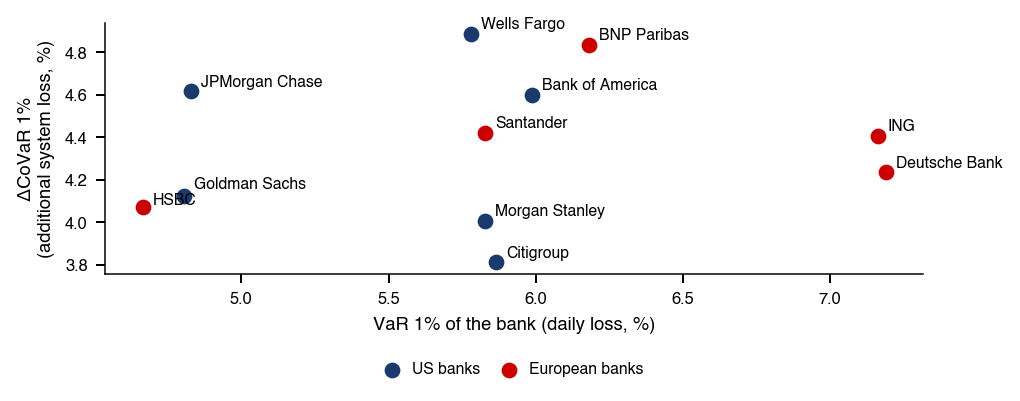

 MFM_ch18_bank_indices

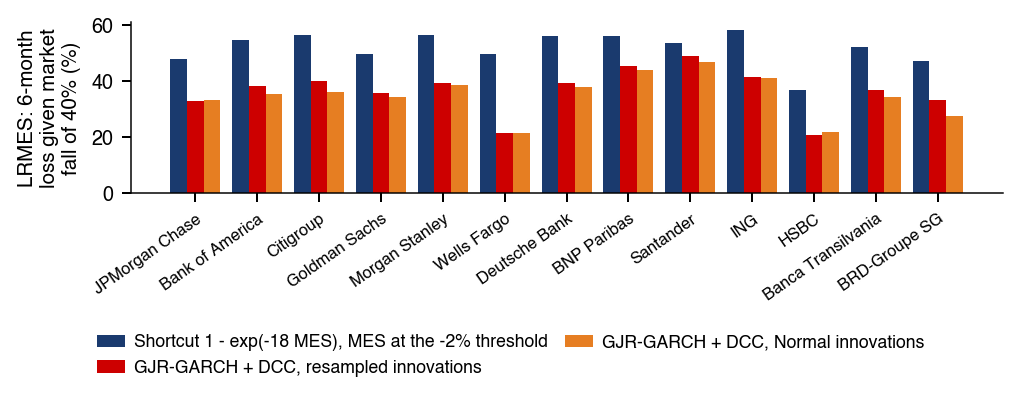
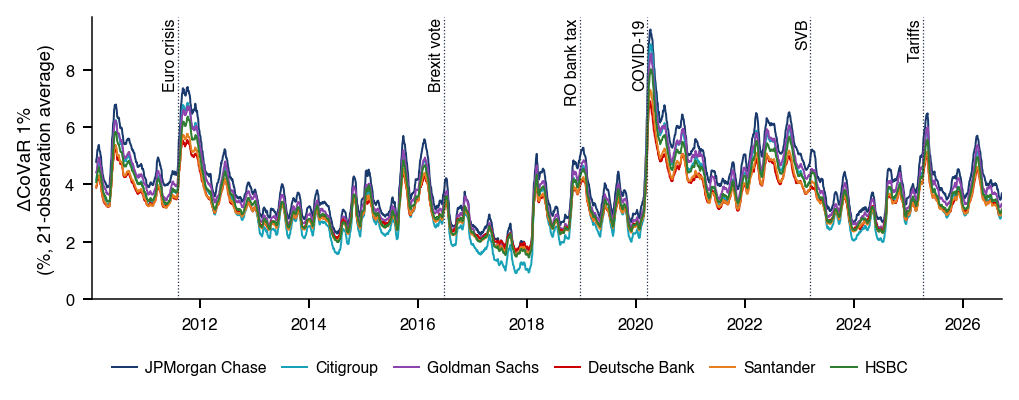
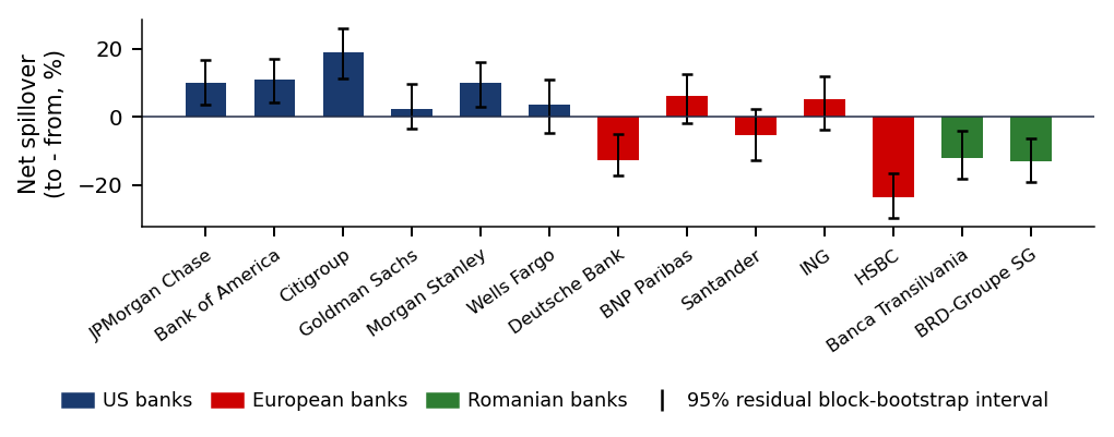
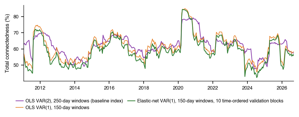
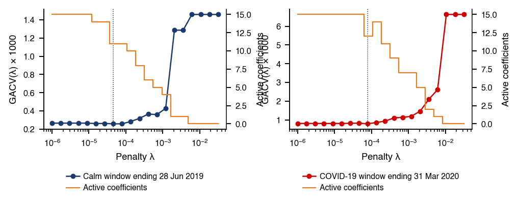
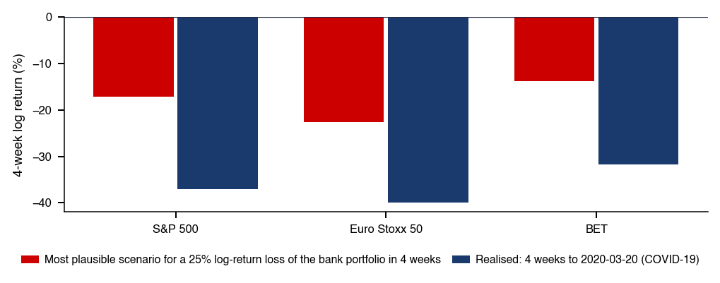
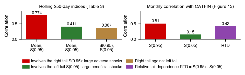
 Financial Risk Meter for Emerging Markets