Chapter 20 (special chapter): Path Signatures and Realised Volatility — a Research Case Study
Daniel Traian PELE
Bucharest University of Economic Studies IDA Institute Digital Assets Blockchain Research Center AI4EFin Artificial Intelligence for Energy Finance Romanian Academy, Institute for Economic Forecasting MSCA Digital Finance
Gu et al. (2024) describe a recent window of a series as a path and summarise it by its path signature. Signature features enter a two-step LASSO (Least Absolute Shrinkage and Selection Operator) regression, and past periods whose path resembles the current one receive a larger weight through a signature kernel. For freight rates, the authors report a more than fivefold accuracy gain over an industry forecast. The chapter asks whether the same method improves forecasts of daily realised variance (RV), where the benchmark is the heterogeneous autoregressive (HAR) model of Corsi (2009) and, above all, its log version, log-HAR.
The transfer is pre-registered: four hypotheses are fixed before the results, and the data are 50 assets from the VOLARE (VOLatility Archive for Realized Estimates, database) archive, 40 of them stocks. Each component of the method is tested separately, so that any gain can be attributed either to the features or to the weights. The comparisons use the QLIKE (quasi-likelihood) loss, asset-by-asset Diebold–Mariano tests and the Holm and Benjamini–Hochberg corrections for multiple testing.
The result is null. At the one-day horizon, Sig-L, the model with signature features, has a mean QLIKE loss 0.4% higher than log-HAR. Sig-L is significantly better than log-HAR on 3 of 50 assets without correction and on a single one after the Holm correction, while about 2.5 raw rejections are expected by chance alone. At one week and one month, the full model, Sig-LK, has a QLIKE loss 28.0% and 92.9% higher than log-HAR. The strongest effect in the study is the oldest one: log-HAR is significantly better than HAR in levels on 21 of 50 assets at one day, without correction. The chapter shows, through ablations and the mechanism, why the method does not transfer.
Ratio of each model's mean QLIKE loss to that of the HAR model, for each of the 50 assets; a ratio below 1 means a more accurate model than HAR. The boxes span the interquartile range across assets, the line in the box is the median and the diamond is the mean. Interactive chart: “QLIKE Relative to HAR, Asset by Asset” →
What you will be able to do
Compute the signature of a piecewise-linear path and its Lévy area.
Compute signature features and kernel weights for a volatility forecast.
Interpret forecast comparisons across many assets, with Diebold–Mariano tests, model confidence sets and Holm and Benjamini–Hochberg corrections.
Interpret the result of a pre-registered transfer to a new domain, including a null result together with its mechanism.
The Further Topics and the Appendix are reading for familiarisation.
Chapter plan
Route and MotivationThe chapter's question, the two components of the method and the HAR benchmark.
AppendixFeatures, estimation, evaluation periods and checks.
Route and Motivation
The chapter tests whether a forecasting method published for freight rates improves forecasts of daily realised variance. The method has two ingredients, signature features of a recent data window and kernel weights that favour similar past windows, and each is tested on its own against the HAR family of benchmarks. The transfer is pre-registered: the hypotheses, the panel and the tests are fixed before the results are seen.
Does a Method Built for Freight Rates Improve Volatility Forecasts?
The method of Gu et al. (2024) was developed to forecast freight rates at Amazon. The chapter asks whether it also improves forecasts of realised variance, using 50 assets from VOLARE (VOLatility Archive for Realized Estimates) (Cipollini et al., 2026). The question is one of transfer: a method that works in one domain is moved to another, with a design fixed in advance.
The chapter develops four skills:
To compute the signature of a piecewise-linear path and its Lévy area.
To compute signature features and kernel weights for a volatility forecast.
To interpret forecast comparisons on many assets, with Diebold–Mariano (DM) tests, model confidence sets and the Holm and Benjamini–Hochberg (BH) corrections.
To interpret the result of a pre-registered transfer, including a null result and its mechanism.
Detailed examples are in the Further Topics, after the Conclusions.
In brief
Path Shape and Volatility Forecasts
A research case study: the method of Gu et al. (2024), transferred to daily realised variance
the method was published for freight rates at Amazon
data: 50 assets from VOLARE (VOLatility Archive for Realized Estimates) Cipollini et al. (2026)
Detailed examples and advanced topics are in Further Topics, after the Conclusions
the footer button leads there; the Back button returns to the starting slide
What you should be able to do
Compute the signature of a piecewise-linear path and its Lévy area
Compute signature features and kernel weights for a volatility forecast
Interpret forecast comparisons on many assets
with Diebold–Mariano (DM) tests and model confidence sets
with Holm and Benjamini–Hochberg (BH) corrections
Interpret the result of a pre-registered method transfer, including a null result and its mechanism
Further Topics and Appendix: reading for familiarity
Volatility is an input to almost every risk measure of the course: tail-risk measures in Chapter 7, option prices in Chapter 12 and portfolio weights in Chapter 4. Intraday data make the daily variance almost observable through realised variance (RV), the measure of Chapter 9. Volatility forecasting therefore becomes a regression problem with a noisy but model-free target.
The benchmark is hard to beat. The HAR (heterogeneous autoregressive) model of Corsi (2009) uses three averages of past RV, is linear and is estimated by ordinary least squares (OLS) in a second. A new method has to beat HAR out of sample, on many assets and with a proper test, before it can be said to improve volatility forecasts.
In brief
Volatility is an input to almost every risk measure in this course
Gu et al. (2024) describe a recent window of a series as a path and summarise it by its signature. The signature features enter a sparse linear regression, a LASSO (least absolute shrinkage and selection operator) estimated in two steps. Past periods whose path looks like the current one receive more weight through a signature kernel. For freight rates the authors report a more than fivefold accuracy gain over an industry forecast.
The chapter's question is whether the same recipe improves on HAR-type models for realised variance. Because the method combines two ingredients, each is tested separately: a gain can then be attributed either to the features or to the weights, and a loss located in one of them.
In brief
Gu et al. describe a recent window of a series as a path and summarise it by its signature
Signature features enter a sparse linear regression (LASSO, least absolute shrinkage and selection operator, in two steps)
Past periods whose path looks like today’s get more weight (a signature kernel)
They report a more than fivefold accuracy gain over an industry forecast of freight rates
Question: does the same recipe improve on HAR-type models for realised variance?
Each ingredient is tested separately, so that a gain can be attributed to the features or to the weights
Before any model is compared, the target must be defined. This section states the price model behind realised variance, the measurement error of RV and the auxiliary measures in the VOLARE data, and then fixes the forecast target, the alignment of forecasts with targets and the loss functions used to rank the models.
The question is what exactly is forecast, and how intraday data measure the variance of a day. The log price \(p_t\), with time in days, moves by a drift, a diffusion term and jumps:
\[dp_t = \mu_t\,dt + \sigma_t\,dW_t + dJ_t,\]
(20.1)
where \(\mu_t\) is the drift, \(\sigma_t\) the spot volatility, \(W_t\) a Brownian motion and \(J_t\) a pure-jump process, with \(\Delta J_s\) the jump size at time \(s\).
where \(M\) is the number of intraday returns in day \(t\) and \(r_{t,i}\) the \(i\)-th intraday log return; for a US (United States) stock, \(M = 78\) five-minute returns cover the 6.5-hour session. The limit in (20.2) is the quadratic variation of the day: the integrated variance plus the sum of squared jumps.
In brief
Question: what exactly do we forecast, and how do intraday data measure the variance of a day?
The price model: the log price moves by a drift, a diffusion term and jumps
\(M\): number of intraday returns in day \(t\) (for a US stock, 78 five-minute returns in the 6.5-hour session); \(r_{t,i}\): the \(i\)-th intraday log return of day \(t\)
The limit is the quadratic variation of day \(t\): the integrated variance plus the sum of squared jumps
Without jumps and noise, on an equally spaced grid, the limit of RV is the integrated variance \(\mathrm{IV}_t = \int_{t-1}^{t}\sigma_s^2\,ds\), the true variance of day \(t\), and the error is mixed Normal:
where \(\mathrm{IQ}_t\) is the integrated quarticity and \(\mathrm{MN}(0, V)\) a Normal law with a random variance \(V\): given the volatility path, the error is Normal with variance \(2\,\mathrm{IQ}_t/M\).
RV is therefore a noisy measurement of \(\mathrm{IV}_t\), and the noise is largest on volatile days, where \(\mathrm{IQ}_t\) is large. This measurement error is what HARQ, the HAR model with realised quarticity, corrects for. In the other direction, microstructure noise makes very fine sampling biased, and five-minute returns are the standard compromise (Chapter 9).
In brief
Without jumps and noise, on an equally spaced grid, the limit is the integrated variance
\(\mathrm{IV}_t\): integrated variance, the true variance of day \(t\); \(\mathrm{IQ}_t\): integrated quarticity
\(\mathrm{MN}(0, V)\): mixed Normal, a Normal with a random variance \(V\); given the volatility path, the error is Normal with variance \(2\,\mathrm{IQ}_t/M\)
Reading: RV is a noisy measurement of \(\mathrm{IV}_t\)
the noise is largest on volatile days (where \(\mathrm{IQ}_t\) is large)
This is the measurement error that HARQ, the HAR model with realised quarticity, corrects for (HAR section)
Microstructure noise makes very fine sampling biased
five-minute returns are the standard compromise (Chapter 9)
Realised semivariances (Barndorff-Nielsen, Kinnebrock & Shephard, 2010) split RV by the sign of the intraday returns: \(\mathrm{RV}_t^{+} = \sum_i r_{t,i}^2\mathbf{1}\{r_{t,i}>0\}\) is the variance from up-moves and \(\mathrm{RV}_t^{-} = \sum_i r_{t,i}^2\mathbf{1}\{r_{t,i}<0\}\) the variance from down-moves, and they add up to \(\mathrm{RV}_t\).
Realised quarticity estimates \(\mathrm{IQ}_t\), the scale of the measurement error of RV:
The factor \(M/3\) comes from the Normal law: a return with variance \(s^2\) has fourth moment \(3s^4\), and each five-minute variance is about \(\mathrm{IV}_t/M\). The limit requires a continuous, noise-free price and an equally spaced grid; a jump \(\Delta J\) adds about \(M(\Delta J)^4/3\), so raw RQ (Realised Quarticity) is sensitive to jumps.
The factor \(M/3\): a Normal return with variance \(s^2\) has fourth moment \(3s^4\), and each five-minute variance is about \(\mathrm{IV}_t/M\)
The limit needs a continuous, noise-free price and an equally spaced grid; a jump \(\Delta J\) adds about \(M(\Delta J)^4/3\), so raw RQ is jump-sensitive
The target at horizon \(h\) is the average RV over the next \(h\) days,
\[\mathrm{RV}_{t+1:t+h} = \frac{1}{h}\sum_{j=1}^{h}\mathrm{RV}_{t+j}, \qquad h \in \{1, 5, 22\},\]
(20.5)
where \(t\) is the forecast origin, the last day observed, and \(h = 1, 5, 22\) are one day, one week and one month of trading days.
Log models forecast \(y = \ln \mathrm{RV}_{t+1:t+h}\) and return to levels with a variance correction, \(F_t = \exp(\hat y_t + \hat s^2/2)\), where \(F_t\) is the forecast made at \(t\),\(\hat y_t\) the fitted log forecast and \(\hat s^2\) the variance of the regression residuals. The correction follows from \(\mathbb{E}[e^Z] = e^{\mu + s^2/2}\) for \(Z \sim N(\mu, s^2)\); it is exact if the log error is conditionally Normal with constant variance and an approximation otherwise.
For \(h > 1\) consecutive targets overlap, which induces serial dependence through lag \(h-1\) by construction and possibly longer. Every test therefore uses a HAC (heteroskedasticity and autocorrelation consistent) variance.
In brief
The target at horizon \(h\) is the average RV over the next \(h\) days
\(F_t\): forecast of \(\RV_{t+1:t+h}\) made at \(t\); \(\hat y_t\): fitted log forecast; \(\hat s^2\): variance of the regression residuals
\(+\hat s^2/2\): since \(\E[e^Z] = e^{\mu + s^2/2}\) for \(Z \sim N(\mu, s^2)\); exact if the log error is conditionally Normal with constant variance, otherwise an approximation
For \(h > 1\) targets overlap: this induces serial dependence
through lag \(h - 1\) by construction, possibly longer
so every test uses a HAC (heteroskedasticity and autocorrelation consistent) variance
The subscripts play two roles. In the definition of the target, \(t\) is the forecast origin; in the loss and test formulas, the subscript labels a matched evaluation row, which pairs the realised target with the forecast made before that target became observable.
At the one-day horizon, information through Monday's close forecasts Tuesday's RV, and the forecast is stored next to the Tuesday realisation. At the five-day horizon the same origin forecasts the average from Tuesday to the following Monday, and the next origin gives an overlapping target. The forecast comparison tests use the same realised target for both models in each row. The row label is not permission to use that target in estimation.
In brief
In the target definition, the subscript \(t\) is the forecast origin
In loss and test formulas, the subscript labels a matched evaluation row
the realised target
the forecast made before that target became observable
One-day horizon: information through Monday close forecasts Tuesday RV
stored next to the Tuesday realisation
Five-day horizon: the same origin forecasts the average from Tuesday to the following Monday
the next origin gives an overlapping target
Forecast comparison tests use the same realised target for both models in each row
Sharing a row with the forecast does not allow the target to be used in estimation
A loss is robust in the sense of Patton (2011) if, for a conditionally unbiased proxy, the ranking of models by expected loss computed with \(\mathrm{RV}_t\) is the same as with the true variance. Conditional unbiasedness means \(\mathbb{E}_{t-1}[\mathrm{RV}_t] = \sigma_t^2\), where \(\mathbb{E}_{t-1}\) is the expectation given information up to \(t-1\) and \(\sigma_t^2\) the true variance of day \(t\).
The chapter uses two robust losses, written here for \(h = 1\) (for \(h > 1\),\(\mathrm{RV}_t\) is replaced by the target):
MSE (mean squared error) is the squared error. QLIKE (quasi-likelihood loss) is zero only if \(F_t = \mathrm{RV}_t\) and grows faster when the forecast is too low than when it is too high: with \(\mathrm{RV}_t = 1\),\(F_t = 0.5\) gives \(2 - \ln 2 - 1 = 0.307\) and \(F_t = 2\) gives \(0.5 - \ln 0.5 - 1 = 0.193\).
QLIKE depends only on the ratio \(\mathrm{RV}_t/F_t\), so the same proportional error has the same loss on a calm day and on a stormy one, whereas MSE is dominated by a few crisis days. QLIKE is therefore the primary loss and MSE the secondary one.
for a conditionally unbiased proxy, the expected-loss ranking with \(\RV_t\) equals that with the true variance
Conditionally unbiased: \(\E_{t-1}[\RV_t] = \sigma^2_t\), with \(\E_{t-1}\) the expectation given information up to \(t - 1\) and \(\sigma^2_t\) the true variance of day \(t\)
The two robust losses used here (written for \(h = 1\); for \(h > 1\) replace \(\RV_t\) by the target)
MSE (mean squared error): the squared error; QLIKE (quasi-likelihood loss) is zero only if \(F_t = \RV_t\) and grows faster when the forecast is too low than when it is too high
the same proportional error has the same loss on a calm day as on a stormy day
MSE is dominated by a few crisis days
QLIKE is the primary loss, MSE the secondary one
The VOLARE Database
The transfer is tested on a panel from VOLARE, which provides five-minute realised measures for many assets. The section describes the 50 assets in three classes, the variables used and the behaviour of realised volatility across classes.
The question is on which data the transfer is tested, and why on three asset classes. The panel has:
40 American large-cap stocks, 2 January 2015 – 30 January 2026, with 111,440 observations and a median annualised volatility of 17.1%;
5 futures, 28 September 2009 – 30 January 2026, with 21,059 observations and 19.7%;
5 currency pairs, 25 September 2009 – 30 January 2026, with 21,203 observations and 7.3%.
The stocks are 40 members of the Dow Jones 30 and S&P 100 (Standard & Poor's), labelled by ticker, from AAPL (Apple) to XOM (Exxon Mobil). The futures are corn (C), crude oil (CL), the E-mini S&P 500 (ES), gold (GC) and natural gas (NG). The FX (foreign exchange) series are the Australian dollar, euro, British pound, Canadian dollar and Japanese yen against the US dollar.
In brief
Class
Assets
Sample
Observations
Median volatility
American large-cap stocks
40
2 Jan 2015 – 30 Jan 2026
111 440
17.1%
Futures (C, CL, ES, GC, NG)
5
28 Sep 2009 – 30 Jan 2026
21 059
19.7%
FX (AUD, EUR, GBP, CAD, JPY vs USD)
5
25 Sep 2009 – 30 Jan 2026
21 203
7.3%
Question: on which data do we test the transfer, and why on three asset classes?
Assets
Stocks: 40 members of the Dow Jones 30 and S&P 100 (Standard & Poor's), labelled by ticker, from AAPL (Apple) to XOM (Exxon Mobil)
Futures: C = corn, CL = crude oil, ES = E-mini S&P 500, GC = gold, NG = natural gas
FX (foreign exchange): Australian dollar, euro, British pound, Canadian dollar and Japanese yen against the US dollar
Three asset classes guard against a narrow result: a gain that appears in one class only does not show that the method transfers. The median volatility in the table is computed as \(\sqrt{252\,\mathrm{median}(\mathrm{RV}_t)}\) for each asset, then as the median over the class; 252 trading days a year turn a daily variance into an annual one, and the data contain trading days only.
The variables are five-minute RV, the semivariances \(\mathrm{RV}^+\) and \(\mathrm{RV}^-\), realised quarticity (RQ) and the daily open and close prices.
In brief
Three asset classes
a gain that appears in one class only does not show that the method transfers
Median volatility in the table: \(\sqrt{252\,\mathrm{median}(\RV_t)}\) per asset, then the median over the class
252 trading days a year turn a daily variance into an annual one
The chart shows annualised volatility \(\sqrt{252\,\mathrm{RV}_t}\) in percent, as a five-day mean on a log scale, for two assets per class: JPMorgan Chase (JPM) and Nvidia (NVDA) among stocks, the E-mini S&P 500 (ES) and crude oil (CL) among futures, and EURUSD (US dollars per euro) and USDJPY (yen per US dollar) among currencies.
Question for the room We keep the same scale. When ▶ widens the moving-average window of the annualised volatility from 5 to 65 days, what happens to the crude-oil (CL) maximum in the first half of 2020?
Answer
It falls, from 458% (five days ending 22 April 2020) to 152% (65 days ending 3 June 2020). A longer averaging window mixes the extreme values with quieter days. The option “unchanged” confuses the smoothed series with the original observations; “rises” confuses a mean with a sum. With the five-day mean, ES reaches 115% in March, JPM 111% and NVDA 118%, while EURUSD and USDJPY stay near 20%. The median volatility per class is 17.1% for stocks, 19.7% for futures and 7.3% for FX.
All classes share the spike of March 2020, while crude oil peaks in April 2020, so a forecaster must adapt within days. The continuous VOLARE series for CL joins successive contracts: the negative price of 20 April 2020 concerned only the May contract, close to expiry, and the series stays positive.
In brief
Annualised volatility \(\sqrt{252\,\RV_t}\) in %, five-day mean, log scale, two assets per class
stocks: JPM = JPMorgan Chase, NVDA = Nvidia
futures: ES = E-mini S&P 500, CL = crude oil
FX: EURUSD = US dollars per euro, USDJPY = yen per US dollar
All classes share March 2020; crude oil (CL) peaks in April 2020
a forecaster must adapt within days
CL: the continuous VOLARE series joins successive contracts
the negative price of 20 April 2020 concerned only the May contract, close to expiry
On a log scale volatility is persistent, the long memory that HAR approximates. Spikes decay within weeks, so the shape of the recent path may carry information beyond a few averages; this is the possibility that signature features are meant to exploit.
In brief
On a log scale volatility is persistent (the long memory HAR approximates)
Spikes decay within weeks, so the shape of the recent path may carry information
The target is the average RV over 1, 5 or 22 days, measured with error that is largest on volatile days and ranked with the robust QLIKE loss. The panel covers 50 assets in three classes, with a common volatility spike in March 2020.
Benchmarks: the HAR Family
A new method is only interesting if it beats the models already in use. This section presents HAR, its log version and two extensions, and arranges the seven models of the chapter so that the contribution of each ingredient of the transferred method can be isolated.
The question is which simple benchmark must be beaten before a new method is believed. In the HAR model of Corsi (2009), future RV is a linear function of the daily, weekly and monthly averages of past RV:
with \(\mathrm{RV}_t^{(w)} = \frac{1}{5}\sum_{j=0}^{4}\mathrm{RV}_{t-j}\) and \(\mathrm{RV}_t^{(m)} = \frac{1}{22}\sum_{j=0}^{21}\mathrm{RV}_{t-j}\) the weekly and monthly averages up to day \(t\), and \(\varepsilon_{t+h}\) the forecast error.
\(\beta_0\) is the intercept, and \(\beta_d\),\(\beta_w\) and \(\beta_m\), nonnegative in practice, measure how much yesterday, last week and last month weigh; they are estimated by OLS for each horizon \(h\). A sum \(\beta_d + \beta_w + \beta_m\) close to 1 means high persistence. The motivation is a cascade of traders at daily, weekly and monthly frequencies, which mimics long memory with three parameters.
In brief
Question: which simple benchmark must be beaten before we believe a new method?
The HAR model Corsi (2009): future RV is a linear function of the daily, weekly and monthly averages of past RV
\(\RV_t^{(w)}\), \(\RV_t^{(m)}\): weekly (5-day) and monthly (22-day) averages of RV up to day \(t\); \(\varepsilon_{t+h}\): forecast error
\(\beta_0\): intercept; \(\beta_d, \beta_w, \beta_m \ge 0\) in practice: how much yesterday, last week and last month weigh; estimated by OLS for each horizon \(h\)
\(\beta_d + \beta_w + \beta_m\) close to 1: high persistence of volatility
Traders at daily, weekly and monthly frequencies
a cascade that mimics long memory with three parameters
HAR is a restricted AR(22), an autoregression with 22 lags whose coefficients take only three distinct values: \(\phi_1 = \beta_d + \beta_w/5 + \beta_m/22\),\(\phi_{2..5} = \beta_w/5 + \beta_m/22\) and \(\phi_{6..22} = \beta_m/22\), where \(\phi_j\) is the coefficient of \(\mathrm{RV}_{t+1-j}\).
The log-HAR model runs the same regression in logs,
which rules out negative forecasts and is less driven by spikes. Logs of averages are not averages of logs, so this log-HAR is not an exact restricted AR(22) in \(\ln \mathrm{RV}\) (Seminar 20, A7). The HARQ and SHAR (Semivariance HAR model) extensions are in the Appendix.
In brief
HAR is a restricted AR(22): the 22 lag coefficients take only three distinct values
The table lists the seven models. HAR, HARQ and SHAR forecast RV in levels with equal weights: HARQ adds the term \(\mathrm{RV}_t(\mathrm{RQ}_t^{1/2} - \overline{\mathrm{RQ}^{1/2}})\) to HAR, and SHAR replaces \(\mathrm{RV}_t\) by the semivariances \(\mathrm{RV}_t^+\) and \(\mathrm{RV}_t^-\). The four remaining models forecast \(\ln \mathrm{RV}\):
log-HAR with equal weights;
log-HAR-K, the log-HAR regressors with signature-kernel weights;
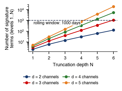
Sig-L, the log-HAR regressors plus 36 non-constant signature terms (39 before dropping constants) selected by a two-step LASSO;
Sig-LK, Sig-L with kernel weights, which is the method of Gu et al. (2024).
In the names, L stands for LASSO and K for kernel weights.
log-HAR, log-HAR-K, Sig-L and Sig-LK form a \(2\times2\) ablation, signature features (yes/no) by kernel weights (yes/no), in which each ingredient is switched on and off separately. log-HAR is the natural baseline for the signature models, because it has the same target and its regressors are among the candidates. The LASSO may also drop log-HAR terms, however, so Sig-L against log-HAR compares two procedures, not only two feature sets.
In brief
Model
Target
Weights
Regressors
HAR
\(\RV\)
equal
\(\RV_t, \RV_t^{(w)}, \RV_t^{(m)}\)
log-HAR
\(\ln \RV\)
equal
the same, in logs
HARQ
\(\RV\)
equal
HAR + \(\RV_t\,(\mathrm{RQ}_t^{1/2} - \overline{\mathrm{RQ}^{1/2}})\)
log-HAR, log-HAR-K, Sig-L and Sig-LK form a \(2 \times 2\) ablation
each ingredient switched on and off separately
signature features (yes/no) \(\times\) kernel weights (yes/no)
Log-HAR is the natural baseline for the signature models
same target, and its regressors are among the candidates
but the LASSO may also drop log-HAR terms
so Sig-L vs log-HAR compares two procedures, not only two feature sets
Path Signatures
The transferred method summarises a window of data by its path signature. This section defines the object: the window as a path, the signature as the sequence of iterated integrals, its computation for piecewise-linear paths through Chen's identity, the Lévy area as a measure of order, and the signature kernel that measures the similarity of two windows.
The question is how to summarise a 22-day window so that the order of the moves is kept, not only their levels. The last \(L\) days of \(d-1\) series are taken, time is added as the first channel (time augmentation) and the points are connected linearly:
a path \(X: [0,1] \to \mathbb{R}^d\) with \(L = 22\) days and \(d = 3\) channels: time, log RV and the cumulative return. Here \(u_i \in [0,1]\) is the rescaled time of the \(i\)-th point and \(r_j = \ln(C_j/O_j)\) the open-to-close log return of day \(j\), with \(O_j\) and \(C_j\) the open and close prices.
A regression on the window sees 22 lags; a path summary sees their order, speed and co-movement. It can distinguish, for example, a window in which RV rose while prices fell from one in which RV rose first and prices fell later.
In brief
Question: how do we summarise a 22-day window so that the order of the moves is kept, not only their levels?
\(L\): window length in days (here 22); \(d\): number of channels (here \(d = 3\): time, log RV, cumulative return); \(u_i \in [0, 1]\): rescaled time of the \(i\)-th point; \(r_j = \ln(C_j/O_j)\): open-to-close log return of day \(j\), with \(O_j\), \(C_j\) the open and close prices
A regression on the window sees 22 lags; a path summary sees their order, speed and co-movement
Example: RV rose while prices fell, or RV rose first and prices fell later
Signatures come from the geometry of loop spaces. Chen (1957) showed that the iterated integrals of a path form an algebra, and Chen (1958) that they determine the path up to reparametrisation and retraced pieces. In the rough path theory of Lyons (1998), the signature is the natural feature set for controlled differential equations: a response to a path depends on it, to first order, only through its signature.
Level 1 of the signature keeps only the total increments of the channels. Integrals over ordered times keep, in addition, the order in which the channels move, which is why the signature is built from iterated integrals. One signature term is an iterated integral of the path along a word of channels:
Here \(X: [a,b] \to \mathbb{R}^d\) is a path of bounded variation (finite total length), for example piecewise linear, and \(X^i_u\) its channel \(i\) at time \(u\). The word \((i_1, \dots, i_k)\) is an ordered list of \(k\) channels with letters in \(\{1, \dots, d\}\), and \(k\) is the level of the term. The integral runs over ordered times \(u_1 < \dots < u_k\), and \(dX^i_u\) is the increment of channel \(i\) at time \(u\), for a linear segment its slope times \(du\).
In brief
Why iterated integrals
level 1 keeps only the total increments
integrals over ordered times keep the order in which the channels move
One signature term is an iterated integral of the path along a word of channels
\(X: [a, b] \to \mathbb{R}^d\): a path of bounded variation (finite total length), e.g. piecewise linear; \(X^i_u\): its channel \(i\) at time \(u\)
Word \((i_1, \dots, i_k)\): an ordered list of \(k\) channels, letters in \(\{1, \dots, d\}\); \(k\) is the level of the term
\(u_1 < \dots < u_k\): the integral runs over ordered times; \(dX^{i}_{u}\): increment of channel \(i\) at time \(u\) (for a linear segment, slope times \(du\))
where \(S^{(k)}\) collects the \(d^k\) terms of level \(k\), one for each word of length \(k\), stored as a tensor (\(\otimes\) is the tensor product). The truncated signature \(\mathrm{Sig}^N(X)\) keeps levels 0 to \(N\);\(N\) is the depth.
Level 1 contains the total increments, \(S^i = X^i_b - X^i_a\). Level 2 contains \(S^{ij} = \int_a^b (X^i_u - X^i_a)\,dX^j_u\), the increments of channel \(j\) weighted by how far channel \(i\) has already moved. Each further level adds one integral and records finer details of the order of the moves.
\(S^{(k)}\): the \(d^k\) terms of level \(k\), one for each word of length \(k\), stored as a \(k\)-dimensional array (a tensor; \(\otimes\): tensor product)
\(\Sig^N(X)\): the truncated signature, levels \(0\) to \(N\); \(N\) is the depth
A linear segment with increment \(\Delta = X_b - X_a \in \mathbb{R}^d\) has the tensor exponential as signature, \(\mathrm{Sig} = \exp_\otimes(\Delta) = (1, \Delta, \Delta^{\otimes2}/2!, \Delta^{\otimes3}/3!, \dots)\), where \(\Delta^{\otimes k}\) is the array of all products \(\Delta^{i_1}\cdots\Delta^{i_k}\), so that a level-\(k\) term is \(\Delta^{i_1}\cdots\Delta^{i_k}/k!\).
Chen's identity (Chen, 1957) states that the signature of two paths run one after the other is the tensor product of their signatures:
where \(X * Y\) is the concatenation, \(Y\) starting where \(X\) ends, and \(A^{(k)}\),\(B^{(k)}\) are level \(k\) of the signatures \(A\) and \(B\), with \(A^{(0)} = B^{(0)} = 1\). Level \(k\) of the whole path collects every way of splitting a word of length \(k\) between the first and the second piece.
In brief
A linear segment with increment \(\Delta \in \mathbb{R}^d\) has the tensor exponential as signature
\(\Delta = X_b - X_a\): the increment of the segment; \(\Delta^{\otimes k}\): the array of all products \(\Delta^{i_1}\cdots\Delta^{i_k}\), so a level-\(k\) term is \(\Delta^{i_1}\cdots\Delta^{i_k}/k!\)
For a piecewise-linear path with \(m\) segments and increments \(\Delta_1, \dots, \Delta_m\),(20.12) gives \(\mathrm{Sig} = \exp_\otimes(\Delta_1)\otimes\cdots\otimes\exp_\otimes(\Delta_m)\). This is the whole algorithm: \(m\) updates, each costing \(O(d^N)\) at depth \(N\).
Rolling windows use Chen's identity in the other direction, to remove an initial piece: \(\mathrm{Sig}(X_{[s,t]}) = \mathrm{Sig}(X_{[a,s]})^{-1}\otimes\mathrm{Sig}(X_{[a,t]})\) for \(a \le s \le t\), where the inverse for \(\otimes\) is the signature of the piece run backwards.
In brief
A piecewise-linear path with \(m\) segments, increments \(\Delta_1, \dots, \Delta_m\)
\(X_{[s,t]}\): the path restricted to \([s, t]\), with \(a \le s \le t\); \((\cdot)^{-1}\): inverse for \(\otimes\), the signature of the piece run backwards
The worked example takes the path \((0,0) \to (1,0) \to (1,2)\), with increments \(\Delta_1 = (1,0)\) and \(\Delta_2 = (0,2)\). Level 1 is \(S^{(1)} = \Delta_1 + \Delta_2 = (1,2)\). Level 2 follows from Chen's identity, \(S^{ij} = \tfrac12\Delta_1^i\Delta_1^j + \Delta_1^i\Delta_2^j + \tfrac12\Delta_2^i\Delta_2^j\), with \(\Delta_m^i\) the component \(i\) of the increment of segment \(m\), and gives \(S^{11} = 1/2\),\(S^{12} = 2\),\(S^{21} = 0\) and \(S^{22} = 2\).
Two checks follow:
\(S^{11} = (\Delta X^1)^2/2\) and \(S^{22} = (\Delta X^2)^2/2\), an instance of the shuffle identity: the product of two level-1 coordinates equals the sum of their two orderings at level 2.
\(S^{12} \neq S^{21}\), because channel 1 moves in the first segment and channel 2 in the second. Level 1 cannot tell this path from the one that goes up first and right second, since both have \(\Delta X = (1,2)\); level 2 tells them apart.
In brief
The path \(X: (0,0) \to (1,0) \to (1,2)\), with increments \(\Delta_1 = (1, 0)\) and \(\Delta_2 = (0, 2)\)
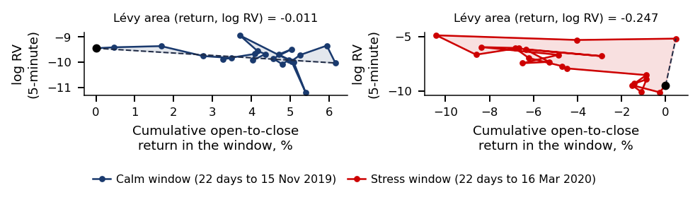
The Lévy area is the antisymmetric part of level 2,
\[A^{ij} = \tfrac12\big(S^{ij} - S^{ji}\big),\]
(20.13)
equal to the signed area between the path, projected on channels \((i,j)\), and its chord, the straight line from start to end. \(A^{ij} > 0\) means that the path turns anticlockwise in the \((i,j)\) plane. The symmetric part, \(\tfrac12(S^{ij} + S^{ji}) = \tfrac12\Delta X^i\Delta X^j\), adds no new information. In the worked example, \(A^{12} = (2-0)/2 = 1\), the area of the triangle between the path and the chord.
As a lead–lag statistic the area needs care. The lead–lag reading requires a positive association: if \(i\) falls and then \(j\) rises, \(i\) moves first, yet \(A^{ij} < 0\). For the channels (return, log RV), a price fall followed by a volatility rise gives \(A < 0\), and so does a price rise followed by a volatility fall. Leverage-type sequences (Chapter 5) are one contributor to a negative area, but the sign alone does not identify them.
In brief
The Lévy area \(A^{ij}\): the antisymmetric part of level 2
The signature kernel is the inner product of the truncated signatures (Király & Oberhauser, 2019), a similarity score between two paths \(X\) and \(Y\) with the same channels:
where \(w\) is a word, \(|w|\) its length and \(S(X)^w\) the term of word \(w\); the leading 1 is level 0. The distance induced by the kernel (Gu et al., Eq. 9) is the squared Euclidean distance between the truncated signatures, \(d_{\mathrm{Sig}}(X,Y) = k_N(X,X) - 2k_N(X,Y) + k_N(Y,Y) = \|\mathrm{Sig}^N(X) - \mathrm{Sig}^N(Y)\|^2\): zero when the two windows have the same signature up to depth \(N\), large when their shapes differ.
Gu et al. (2024) and this chapter use this truncated kernel, with the same depth \(N\) as the features. The untruncated kernel solves a Goursat PDE (partial differential equation) (Salvi et al., 2021), which the paper cites but does not use. The channels are rescaled before the kernel is computed (Appendix); otherwise the channel with the largest units dominates.
In brief
Kernel = inner product of the truncated signatures Király & Oberhauser (2019): a similarity score between two paths
\(X\), \(Y\): two paths with the same channels; \(w\): a word, \(|w|\): its length (level); \(S(X)^{w}\): the term of word \(w\); the leading 1 is level 0
Distance induced by the kernel (Gu et al., Eq. 9)
squared Euclidean distance between the truncated signatures
\(d_{\Sig} = 0\): the two windows have the same signature up to depth \(N\); large \(d_{\Sig}\): different shapes
Gu et al. and this chapter use this truncated kernel, with \(N\) as for the features
The untruncated kernel solves a Goursat PDE (partial differential equation) Salvi et al. (2021); the paper cites it but does not use it
Channels are rescaled before the kernel (Appendix): otherwise the channel with the largest units dominates
Section summary
A window of data becomes a path, and its signature records the increments and the order of the moves level by level. Chen's identity makes the signature of a piecewise-linear path a product of tensor exponentials, the Lévy area turns order into a number, and the signature kernel compares windows by the distance between their truncated signatures.
The Paper: Gu et al. (2024)
Before the method is transferred, the section states exactly what Gu et al. (2024) did and how strong their evidence is: the forecasting problem, the features, the two-step LASSO, the kernel weights, the reported gains and the limits of that evidence.
The question is what exactly the paper did, and how strong its evidence is. Gu et al. (2024) forecast weekly North American truckload rates, nationally and for five regions, in 2018–2022, up to 12 weeks ahead. More than 100 candidate factors were screened down to about 40. The method has been used in Amazon operations since November 2022 and was published at KDD 2024 (Knowledge Discovery and Data Mining, the conference of the Association for Computing Machinery, ACM).
The design is direct: one regression per horizon \(\Delta t\), in weeks, of the rate \(y_{\tau+\Delta t}\) on the features \(\xi_\tau\) observed at week \(\tau\).
In brief
Question: what exactly did the paper do, and how strong is its evidence?
Weekly North American truckload rates, national and five regions, 2018–2022 Gu et al. (2024)
forecast up to 12 weeks ahead
More than 100 candidate factors screened to about 40
In Amazon operations since November 2022; KDD 2024 (Knowledge Discovery and Data Mining, the conference of the ACM, Association for Computing Machinery)
One direct regression per horizon \(\Delta t\) (in weeks; the paper's notation, not an increment \(\Delta\)), \(y_{\tau + \Delta t}\) on the features \(\xi_\tau\) (next slide)
where \(y_{t_i}\) is the rate in week \(t_i\),\(\tau - l \le t_i \le \tau\), and \(l\) the lookback in weeks. The external factors bring the level and information from outside the series; the signature brings the shape of the recent path.
with \(\theta\) the coefficient vector, \(\|\theta\|_1 = \sum_j|\theta_j|\),\(w_\tau \ge 0\) the weight of week \(\tau\), equal or given by the kernel, and \(\lambda \ge 0\) the penalty: a larger \(\lambda\) generally favours sparser solutions, and \(\lambda = 0\) gives weighted OLS. The second step (Eq. 15) refits by weighted OLS on the selected support, the nonzero coefficients of the first step.
The refit is needed because the LASSO shrinks the kept coefficients towards zero; OLS after selection removes this penalty-induced shrinkage on the selected support (Belloni & Chernozhukov, 2013), but not selection or omitted-variable bias. The paper calls the method "adaptive" because of the weights \(w_\tau\), not in the sense of the adaptive LASSO of Zou (2006). In this chapter \(\lambda\) is chosen in each training window as the support with the smallest BIC (Bayesian Information Criterion) along the LARS (Least Angle Regression) path (Efron et al., 2004); details are in the Appendix.
\(\theta\): coefficient vector, \(\|\theta\|_1 = \sum_j |\theta_j|\); \(w_\tau \ge 0\): weight of week \(\tau\) (equal, or from the kernel, next slide)
\(\lambda \ge 0\): penalty; a larger \(\lambda\) generally favours sparser solutions; \(\lambda = 0\) is weighted OLS
Step 2, refit by weighted OLS on the selected support only, the nonzero coefficients of step 1 (Eq. 15)
The kernel weights start from the distance of each past window to the last window with an observed target (Eq. 11), \(\delta_\tau = d_{\mathrm{Sig},N}(z_{\tau-l:\tau},\, z_{t-\Delta t-l:t-\Delta t})\). Here \(z_\tau = (x_\tau, y_{\tau+\Delta t})\) are the pairs of predictors and later target, not the features \(\xi_\tau\) (Algorithm 1), \(t\) is the current week and \(t - \Delta t\) the last week whose target \(y_t\) is already observed. The weights are a softmax with temperature \(\gamma \ge 0\) (Eq. 12):
where \(s\) runs over all training weeks, so the weights sum to 1. Similar windows, with small \(\delta_\tau\), get more weight; \(\gamma = 0\) gives ordinary equal-weight regression and \(\gamma \to \infty\) uses only the most similar past window.
The idea is a nearest-neighbour scheme inside a regression: learn from the past periods that looked like today. Its cost is a smaller effective sample, measured by Kish's \(n_{\mathrm{eff}} = 1/\sum_\tau w_\tau^2\), which equals \(n\) for equal weights \(1/n\) and 1 if one week takes all the weight.
In brief
Distance of each past window to the last window with an observed target (Eq. 11)
\begin{equation*} \delta_\tau = d_{\Sig, N}\big(z_{\tau - l : \tau},\; z_{t - \Delta t - l : t - \Delta t}\big) \end{equation*}
\(z_\tau = (x_\tau, y_{\tau+\Delta t})\): the pairs of predictors and later target, not the features \(\xi_\tau\) (Algorithm 1); \(z_{\tau - l : \tau}\): their path over \(l\) weeks
\(t\): the current week; \(t - \Delta t\): the last week whose target \(y_t\) is already observed; \(d_{\Sig, N}\): the signature distance at depth \(N\)
Softmax weights with temperature \(\gamma \ge 0\) (Eq. 12): similar windows (small \(\delta_\tau\)) get more weight
\(s\): runs over all training weeks, so the weights sum to 1; \(\gamma = 0\): ordinary (equal-weight) regression; \(\gamma \to \infty\): only the most similar past window
A nearest-neighbour idea inside a regression: learn from the past periods that looked like today
Cost of the idea: fewer effective observations, \(n_{\mathrm{eff}} = 1 / \sum_\tau w_\tau^2\) (Kish); \(n_{\mathrm{eff}} = n\) for equal weights \(1/n\), \(n_{\mathrm{eff}} = 1\) if one week takes all the weight
For national rates three months ahead, April–November 2021 (Table 1), the paper reports a relative error \(|y - \hat y|/|y|\), with \(y\) the realised rate and \(\hat y\) its forecast, of about 1–2%, against 13–27% for the industry forecast: "more than fivefold". Over horizons of 1–12 weeks (Table 2) the errors are 1.06–2.60% nationally and 1.05–5.69% by region, with an estimated annual saving of about 50 million dollars.
The kernel ablation (Table 3) uses six weekly values, 31 October – 5 December 2021, for one region: errors reach 9.85% without the kernel and 5.15% with it. What the result supports is a comparison of procedures against a single commercial forecast, without standard errors.
In brief
National rates, three months ahead, April–November 2021 (Table 1)
There is one benchmark, an unnamed commercial forecast, with no ARIMA (autoregressive integrated moving average) model, no LASSO without signatures and no random walk.
The evaluation is short: a few months and a few series, without standard errors or a test of equal accuracy.
The tuning is undisclosed: the lookback \(l\), the depth \(N\), the temperature \(\gamma\), the penalty \(\lambda\) and how they were chosen.
None of this makes the method wrong; it makes the evidence thin, which is why the method is tested elsewhere. The order is replication before extension, as in Chapter 19.
In brief
One benchmark: an unnamed commercial forecast
no ARIMA (autoregressive integrated moving average) model
no LASSO without signatures, no random walk
Short evaluation: a few months, a few series, no standard errors, no test of equal accuracy
Undisclosed tuning: \(l\), \(N\), \(\gamma\), \(\lambda\) and how they were chosen
None of this makes the method wrong; it makes the evidence thin
The signature of the time-augmented recent path of the target;
The two-step LASSO with weights and a direct regression per horizon;
Softmax weights \(\exp(-\gamma\,\delta_\tau)\) with the truncated signature kernel.
The adaptations follow from the new target. RV is daily and noisy rather than a weekly rate, so the models work in logs, inference is HAC and the losses are robust. The external factors \(x_\tau\) are replaced by the log-HAR terms, which carry the level.
The kernel is also adapted. It compares the paths (time, \(\ln\mathrm{RV}\), return) ending at \(\tau\) and at the origin \(t\), updated every 5 days, rather than the pairs \((x_\tau, y_{\tau+\Delta t})\) ending at \(t - \Delta t\). The choices the paper did not disclose, \(l\),\(N\),\(\gamma\) and \(\lambda\), are fixed in advance, and strong benchmarks with formal tests replace the single commercial forecast.
In brief
Transfers
Signature of the time-augmented recent path of the target
Two-step LASSO with weights, direct regression per horizon
Softmax weights \(\exp(-\gamma\,\delta_\tau)\) with the truncated signature kernel
Must be adapted
Daily, noisy target instead of weekly rates: logs, HAC inference, robust losses
External factors \(x_\tau\) replaced by the log-HAR terms (they carry the level)
The kernel compares the paths (time, \(\ln\RV\), return) ending at \(\tau\) and at \(t\)
updated every 5 days
not the pairs \((x_\tau, y_{\tau+\Delta t})\) ending at \(t - \Delta t\)
Undisclosed choices (\(l\), \(N\), \(\gamma\), \(\lambda\)) fixed ex ante
strong benchmarks and formal tests replace the single commercial forecast
The Transfer Design (Pre-Registered)
A method with several tuning choices can always be made to look good on some asset, horizon or period. The design therefore fixes, before any result is seen, the hypotheses, the tuning rule for the kernel temperature, the rolling estimation scheme and the evaluation protocol, and it discloses the one change made after a test run.
The question is what must be fixed before the results, so that a gain cannot be found by searching. Four hypotheses are stated:
H1 (features): signature terms add information beyond log-HAR, tested by Sig-L against log-HAR, with the same target and the same equal weights.
H2 (weights): kernel weights improve a given regression, tested by Sig-LK against Sig-L and log-HAR-K against log-HAR.
H3 (method): the full method of Gu et al. (2024) beats the HAR family, tested by Sig-LK against HAR and against log-HAR and by the model confidence set (MCS) of all seven models.
H4 (stress): any gain is larger in stress periods, the COVID-19 crash and the US tariff shock of 2–30 April 2025, where similar past windows should matter most.
In brief
Question: what do we fix before the results, so that a gain cannot be found by searching?
H1 (features): signature terms add information beyond log-HAR
Test: Sig-L vs log-HAR, same target, same equal weights
H2 (weights): kernel weights improve a given regression
Tests: Sig-LK vs Sig-L and log-HAR-K vs log-HAR
H3 (method): the full method of Gu et al. beats the HAR family
Sig-LK vs HAR and vs log-HAR
model confidence set, MCS, of all seven models
H4 (stress): any gain is larger in stress periods
COVID-19 crash, 2–30 April 2025, the US tariff shock
where similar past windows should matter most
Kernel Temperature: One Choice per Class, on a Validation Block
where \(\delta_\tau\) are the kernel distances of the training days to the current window and \(c > 0\) is a dimensionless constant, the only tuning parameter. With \(c = 1\), a window at the median distance gets weight \(e^{-1}\) relative to an identical one; a larger \(c\) concentrates the weights.
\(c\) is chosen from the grid \(\{0.5, 1, 2, 4\}\) per horizon and asset class, on the first 250 forecast days of each asset pooled within the class. The criterion is the class mean of QLIKE\((c)\) divided by the asset's average over the grid. Evaluation starts after the last validation target of the class, so no tuning target postdates an evaluated origin.
For the 40 stocks the smallest temperature, \(c = 0.5\), wins at every horizon for Sig-LK, which gives the most nearly equal weights. For futures and FX the choice changes with the horizon, a sign of a flat, noisy criterion; all values are in the Appendix.
In brief
Scale-free temperature, set in every training window
The diagram shows the rolling scheme. The models are re-estimated every 5 trading days on the last 1,000 complete pairs \((\xi_\tau, y_{\tau+h})\) with \(\tau + h \le t\), so that every target used in estimation is observed at the origin \(t\). Between re-estimations the coefficients are fixed while the regressors are updated daily, and the forecasts from \(t\) to \(t+4\) use the same estimates. The kernel distances are recomputed at each re-estimation, against the window ending at the origin \(t\).
The question is whether the loss difference between two models exceeds sampling noise. For each asset and horizon the mean QLIKE and MSE of two models are compared by the DM (Diebold–Mariano) test of equal predictive accuracy (Diebold & Mariano, 1995); the relative error of the paper is reported only descriptively (Appendix). The statistic is
where \(L\) is the loss (QLIKE or MSE), \(F^A_t\) and \(F^B_t\) the forecasts of models \(A\) and \(B\),\(\bar d\) the mean loss differential over the \(T\) evaluation days and \(\hat\Omega\) the long-run variance of \(d_t\) (Further Topics).
Under \(H_0: \mathbb{E}[d_t] = 0\), DM is approximately \(N(0,1)\), and \(\mathrm{DM} < -1.645\) means that model \(A\) is significantly more accurate at 5%, one-sided. Because estimation is rolling, the test is read as the unconditional GW (Giacomini–White) test; the conditional GW test also asks whether \(d_{t-h}\) predicts \(d_t\), with instruments \((1, d_{t-h})\)(Giacomini & White, 2006).
In brief
Question: is the loss difference between two models larger than sampling noise?
The DM test compares two models, but here there are seven and no benchmark chosen in advance. The model confidence set of Hansen, Lunde & Nason (2011) at 90% is the set of models that contains the best one with probability at least 90%. It is built by elimination: while the \(T_{\max}\) statistic, the largest standardised gap between a model's mean loss and the average over the models still in the set, rejects equal accuracy, the worst model is dropped.
The p-values come from the stationary bootstrap of Politis & Romano (1994), with 1,000 replications and a mean block length of \(\max(h, 10)\) days. The loss series of all models are resampled jointly, to keep the dependence across models.
In brief
Why a set of models: the DM test compares two models
here there are seven and no benchmark chosen in advance
MCS at 90% Hansen, Lunde & Nason (2011): the set of models that contains the best one with probability at least 90%
Built by elimination: while the \(T_{\max}\) statistic (the largest standardised gap between a model’s mean loss and the average over the models still in the set) rejects equal accuracy, drop the worst model
\(p\)-values by the stationary bootstrap Politis & Romano (1994), 1000 replications, mean block length \(\max(h, 10)\) days
The loss series are resampled jointly, to keep the dependence across models
Evaluation Protocol (3/3): Panel Test and Corrections
The panel test applies DM to the cross-sectional mean loss differential, one series with one value per date. In addition, the assets out of 50 with significantly better results are counted, with two corrections:
The Holm correction (Holm, 1979) controls the FWER (family-wise error rate), the probability of at least one false rejection;
The BH procedure of Benjamini & Hochberg (1995) controls the FDR (false discovery rate), the expected share of false rejections among the rejections.
Results are also reported for subperiods: 20 February – 30 April 2020 (the COVID-19 crash), 2–30 April 2025 (the US tariff shock) and all other days. The evaluation periods by class are in the Appendix.
In brief
Panel: DM test on the cross-sectional mean loss differential (one series, one value per date)
Count the assets (of 50) with significantly better results
The Holm correction Holm (1979) controls the FWER (family-wise error rate, the probability of at least one false rejection)
BH Benjamini & Hochberg (1995) controls the FDR (false discovery rate, the expected share of false rejections among the rejections)
Subperiods (evaluation periods by class: Appendix)
The pre-registration included the insanity filter of Bollerslev, Patton & Quaedvlieg (2016) (BPQ) on all models. A test run of the code on JPM, one asset and before any panel result, showed the filter replacing correct crash forecasts by the calm in-sample mean: on 12 March 2020 the realised next-day RV of JPM was about 40 times the filtered HAR forecast.
The rule was therefore changed before the models were estimated on the 50-asset panel. The primary results impose positivity only: a forecast \(\le 0\) is replaced by the in-sample mean. The BPQ filter is kept as a robustness check and reported in full.
In brief
Pre-registered: the BPQ (Bollerslev–Patton–Quaedvlieg) insanity filter on all models: a forecast outside the in-sample range of the target becomes the in-sample mean
A test run of the code on JPM (one asset, before any panel result) showed it replacing correct crash forecasts by the calm in-sample mean
On 12 March 2020 the realised next-day RV of JPM was about 40 times the filtered HAR forecast
Changed before estimating the models on the 50-asset panel
primary results with positivity only
a forecast \(\le 0\) becomes the in-sample mean
The BPQ filter is kept as a robustness check and reported in full
Section summary
The design fixes four hypotheses, one tuning constant per class chosen on a validation block, a rolling scheme with re-estimation every 5 days and an evaluation protocol of DM tests, model confidence sets and Holm and BH corrections. The single change to the pre-registered plan, the forecast filter, was made before any panel result and is disclosed.
Results
The section reports the pre-registered comparison on the 50 VOLARE assets: the QLIKE losses of every model relative to HAR, the asset-by-asset Diebold–Mariano (DM) tests with the Holm and Benjamini–Hochberg (BH) corrections, the model confidence sets, the panel tests, the COVID-19 crash and the kernel weights at the height of the crash. The main comparison is Sig-LK, the full method of Gu et al. (2024), against log-HAR, the simplest model in logs; HAR in levels is the benchmark that every ratio is expressed against.
Question for the room At h = 1, across all 50 assets, the mean QLIKE ratio of Sig-L to HAR is 0.886. We switch the benchmark from HAR to log-HAR. Where will the mean of the Sig-L ratios lie?
Answer
Above 1: the mean Sig-L/log-HAR ratio is 1.004, so Sig-L has a slightly higher relative loss in this sample; for Sig-LK, 1.045. When the benchmark changes, the page recomputes the ratio of each asset and then averages; it does not divide the two means. A value of 1 is guaranteed only for the benchmark compared with itself. Relative to HAR, the means are 0.883 for log-HAR, 0.885 for log-HAR-K and 0.886 for Sig-L. These means are not a significance test.
The question is whether the method of Gu et al. (2024) beats the HAR models and, above all, log-HAR. For each asset the chart reports the ratio of the model's mean QLIKE loss to the mean QLIKE loss of HAR, so that a value below 1 means a more accurate forecast than HAR. The boxes give the interquartile range over the 50 assets, the line the median, the diamond the mean, and the whiskers extend to 1.5 interquartile ranges.
The ratios are averaged over assets with equal weights, here as in the ablation and the filtered results. The mean of the ratios is not the ratio of the means, so a change of benchmark produces new per-asset ratios rather than a rescaling. Medians describe a typical asset, while means remain sensitive to a few large losses.
In brief
Question: does the method of Gu et al. beat the HAR models and, above all, log-HAR?
Ratio for each asset: mean QLIKE of the model over mean QLIKE of HAR; below 1: more accurate than HAR
Boxes: interquartile range over the 50 assets; line: median; diamond: mean; whiskers: 1.5 interquartile ranges
Ratios are averaged over assets with equal weights
here, in the ablation and in the filtered results
the mean of the ratios is not the ratio of the means
so a new benchmark means new per-asset ratios
Medians describe a typical asset; means remain sensitive to a few large losses
At the one-day horizon, \(h = 1\), the mean ratios of log-HAR, log-HAR-K and Sig-L are close: 0.883, 0.885 and 0.886. The features alone, Sig-L against log-HAR, raise the QLIKE loss by 0.4%, so the 36 extra signature features bring no gain; the features together with the kernel weights, Sig-LK against log-HAR, raise it by 4.5%.
At \(h = 5\) and \(h = 22\) days Sig-LK falls behind log-HAR, by 28.0% and 92.9%. Its median ratios to HAR, 0.997 and 0.968, are much better than its means, so a few assets and days drive the loss. Without the return channel in the path, Sig-LK reaches ratios of 0.878 and 0.770, close to those of log-HAR, 0.871 and 0.765.
HARQ and SHAR lose to HAR in levels here, because the main design does not apply the BPQ (Bollerslev–Patton–Quaedvlieg) filter; the filter rescues HARQ (Appendix). The first verdict is that the method does not beat the simplest log model. A near-tie is not a proof of equal accuracy, and the result supports a comparison of procedures.
In brief
\(h = 1\): log-HAR, log-HAR-K and Sig-L are close (0.883, 0.885, 0.886)
Features alone (Sig-L vs log-HAR): +0.4% in QLIKE, so 36 extra features bring no gain
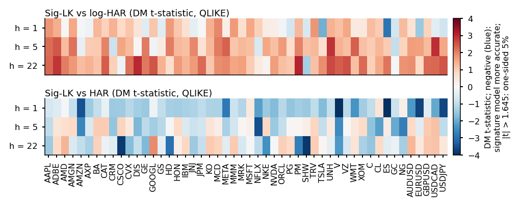
The table counts, for each comparison and horizon, the assets on which the first model is significantly better and significantly worse under QLIKE, each as raw/Holm/BH counts. The test is the one-sided DM test at 5% of Diebold & Mariano (1995), and the family for the corrections is the 50 assets. The DM test needs finite moments of order \(2 + \delta\) and weak dependence of the QLIKE loss differential \(d_t\), not of the returns, and forecasts close to zero can violate these conditions.
The two corrections control different error rates:
The procedure of Holm (1979) controls the family-wise error rate (FWER), the probability of at least one false rejection, under any dependence.
The procedure of Benjamini & Hochberg (1995) controls the false discovery rate (FDR), the expected share of false rejections among the rejections, under independence or under positive regression dependence on a subset (PRDS) (Benjamini & Yekutieli, 2001).
In brief
Comparison (QLIKE)
\(h = 1\)
\(h = 5\)
\(h = 22\)
Sig-LK vs log-HAR
2/0/0 \(|\) 5/0/0
0/0/0 \(|\) 15/0/2
0/0/0 \(|\) 27/1/16
Sig-L vs log-HAR
3/1/1 \(|\) 5/0/0
0/0/0 \(|\) 9/0/0
1/0/0 \(|\) 21/0/0
log-HAR-K vs log-HAR
3/0/0 \(|\) 3/0/0
3/0/0 \(|\) 1/0/0
5/0/0 \(|\) 6/0/0
Sig-LK vs Sig-L
2/0/0 \(|\) 5/0/0
0/0/0 \(|\) 5/0/0
2/0/0 \(|\) 10/0/0
Sig-LK vs HAR
12/5/6 \(|\) 0/0/0
7/1/1 \(|\) 0/0/0
8/2/4 \(|\) 1/0/0
log-HAR vs HAR
21/5/17 \(|\) 0/0/0
23/13/20 \(|\) 0/0/0
42/25/42 \(|\) 0/0/0
Cell: significantly better on raw/Holm/BH assets \(|\) significantly worse on raw/Holm/BH assets
one-sided DM at 5%, family of 50 assets
the DM test needs finite moments of order greater than 2 and weak dependence of the QLIKE loss differential \(d_t\), not of the returns; forecasts close to zero can violate them
Holm controls the FWER under any dependence
BH controls the FDR under independence or PRDS (positive regression dependence on a subset) Benjamini & Yekutieli (2001)
For H1, the hypothesis that the signature features add information, Sig-L beats log-HAR on 3 of the 50 assets at \(h = 1\) before correction and on 1 after Holm, while about 2.5 raw wins are expected by chance alone. At the same horizon Sig-L loses to log-HAR on 5 assets before correction and on none after Holm.
For H2, the hypothesis that the kernel weights help, neither log-HAR-K against log-HAR nor Sig-LK against Sig-L shows a Holm-significant difference at any horizon. Against HAR at \(h = 1\), Sig-LK wins on 12 assets, but log-HAR alone wins on 21. The benchmark must therefore isolate the idea being tested: a comparison with HAR credits the signature with a gain that belongs to the log transform.
In brief
H1 (signatures): Sig-L beats log-HAR on 3 of 50 assets at \(h = 1\) raw, 1 after Holm
about 2.5 raw wins are expected by chance
Also at \(h = 1\), Sig-L loses to log-HAR on 5 assets raw and on none after Holm
H2 (weights): log-HAR-K vs log-HAR and Sig-LK vs Sig-L: no Holm-significant difference at any horizon
Against HAR at \(h = 1\), Sig-LK wins on 12 assets, but log-HAR alone wins on 21
Question for the room We keep QLIKE and all 50 assets. When ▶ raises the MCS confidence level from 90% to 99%, what happens to the share of assets for which Sig-LK stays in the set?
Answer
It rises or stays the same. The elimination threshold α falls from 0.10 to 0.01, and the page keeps the models with an MCS p-value above the threshold, so it eliminates fewer. For Sig-LK, the shares go from 100%, 94% and 88% to 100%, 100% and 100% at h = 1, 5 and 22; for log-HAR, from 100%, 98% and 98% to 100%. A higher confidence level does not mean a more restrictive selection. Membership of the MCS does not establish equal accuracy: at 90%, the four log models are rarely separated, while HAR, HARQ and SHAR are excluded for a fifth to a third of the assets.
The model confidence set (MCS) of Hansen, Lunde & Nason (2011) is the set of models that cannot be rejected as the best at a given level. The chart shows, for each model, the share of the 50 assets in which it belongs to the 90% MCS under QLIKE at \(h = 1\), 5 and 22. log-HAR belongs to it for 100%, 98% and 98% of the assets, and Sig-LK for 100%, 94% and 88%. The MCS needs the same moment and dependence conditions on the loss differentials between models as the DM test.
The MCS rarely separates the four log models. HAR, HARQ and SHAR are excluded for a fifth to a third of the assets, so the level target is the clearest loser.
In brief
Share of the 50 assets in which each model belongs to the 90% MCS under QLIKE (\(h = 1, 5, 22\))
log-HAR 100%, 98%, 98%
Sig-LK 100%, 94%, 88%
the MCS on QLIKE needs the same conditions as the DM test on the loss differentials between models, not on the returns
The MCS rarely separates the four log models
HAR, HARQ and SHAR are excluded for a fifth to a third of the assets
Under the mean squared error (MSE) almost every model stays in the set. Differences in mean MSE loss have large standard errors, because the squared errors of variance forecasts are dominated by a few extreme days.
The panel test pools the evidence: for each day the series is the mean QLIKE differential over the assets available that day, an unbalanced panel, and the DM statistic is computed on this series, with a negative \(t\) meaning that the first model is better. Pooled, only the log transform is clearly significant: log-HAR beats HAR with \(t = -3.09\),\(-3.95\) and \(-4.50\) at the three horizons, all with \(p < 0.001\).
Sig-L against log-HAR at \(h = 1\) gives \(t = -1.91\), significant in a single one-sided test (\(p = 0.028\)). The result is fragile:
For the 40 stocks alone the sign flips, to \(t = +1.72\) against Sig-L;
After a Holm correction over the three horizons, with threshold \(0.05/3 \approx 0.017\), it is no longer significant;
It disappears in the balanced panel of the next slide.
The conditional test of Giacomini & White (2006) (GW), Sig-LK against log-HAR, gives 0, 0 and 0 Holm rejections out of 50 assets.
In brief
Comparison: DM \(t\) (one-sided \(p\))
\(h = 1\)
\(h = 5\)
\(h = 22\)
Sig-LK vs log-HAR
+1.45 (0.927)
+1.68 (0.953)
+1.80 (0.964)
Sig-L vs log-HAR
-1.91 (0.028)
+1.48 (0.931)
+1.51 (0.935)
log-HAR-K vs log-HAR
+1.89 (0.971)
+0.40 (0.654)
+1.92 (0.973)
Sig-LK vs Sig-L
+1.74 (0.959)
+0.98 (0.837)
-0.77 (0.221)
log-HAR vs HAR
-3.09 (\(<\)0.001)
-3.95 (\(<\)0.001)
-4.50 (\(<\)0.001)
Series: the mean QLIKE differential over the assets available that day (unbalanced panel)
negative \(t\) = first model better
the DM test needs finite moments of order greater than 2 and weak dependence of the QLIKE loss differential \(d_t\), not of the returns; forecasts close to zero can violate them
Pooled, only the log transform is clearly significant
Sig-L vs log-HAR at \(h = 1\): significant in a single one-sided test (\(p = 0.028\)) in the unbalanced panel
in the balanced panel the result disappears (next slide)
For the 40 stocks alone the sign flips: \(t = +1.72\) against Sig-L
After a Holm correction over the three horizons (threshold \(0.05/3 \approx 0.017\)) it is no longer significant
Conditional GW test, Sig-LK vs log-HAR: 0, 0 and 0 Holm rejections out of 50
The unbalanced panel averages the assets available each day: futures and foreign exchange (FX) from 2014, the stocks only from 27 January 2020. Differences between asset classes are thus mixed with differences between periods. The balanced panel keeps all 50 assets but only the days on which all of them have forecasts, 1,511 days at \(h = 1\), from 27 January 2020 to 29 January 2026.
On the balanced panel Sig-L against log-HAR at \(h = 1\) gives \(t = +0.75\)(\(p = 0.773\)), against \(t = -1.91\)(\(p = 0.028\)) in the unbalanced panel; on the common calendar only the panel of the 5 futures favours Sig-L (\(t = -4.03\)). The advantage of log-HAR over HAR remains, with \(t\) between −4.76 and −2.21.
In brief
Comparison: DM \(t\) (one-sided \(p\))
\(h = 1\)
\(h = 5\)
\(h = 22\)
Sig-LK vs log-HAR
+1.19 (0.884)
+1.61 (0.946)
+1.41 (0.921)
Sig-L vs log-HAR
+0.75 (0.773)
+1.49 (0.932)
+1.24 (0.892)
log-HAR vs HAR
\(-\)2.21 (0.014)
\(-\)2.51 (0.006)
\(-\)4.76 (\(<\)0.001)
The unbalanced panel averages the assets available each day: futures and FX from 2014, the stocks only from 27 Jan 2020
differences between classes are thus mixed with differences between periods
The balanced panel: all 50 assets, only the days on which all of them have forecasts (1511 days at \(h = 1\), 27 Jan 2020 – 29 Jan 2026)
Sig-L vs log-HAR at \(h = 1\): \(t = +0.75\) (\(p = 0.773\)), against \(t = -1.91\) (\(p = 0.028\)) in the unbalanced panel
on the common calendar only the panel of the 5 futures favours Sig-L (\(t = -4.03\))
The advantage of log-HAR over HAR remains: \(t\) between \(-\)4.76 and \(-\)2.21
Question for the room At h = 1, which of the three displayed forecasts captures the size of the target jump for the 11 March 2020 origin of JPM volatility?
Answer
None. At this origin, the next-day target is about 139%, while the forecasts are 59% (HAR), 49% (log-HAR) and 60% (Sig-LK): all strongly underestimate the jump. The somewhat faster later reaction of Sig-LK in mid-March and the later overshooting of the target by HAR do not show that either anticipated this jump. The raw HAR forecast turns negative in late March; the chart shows the value after the positivity rule (the mean target of the training window), and the 7 replaced origins are marked with ×.
The chart shows, for JPMorgan Chase (JPM) from February to May 2020, the one-day forecasts of the models and the target, both as annualised volatility in percent, \(\sqrt{252F_t}\) and \(\sqrt{252\,\mathrm{RV}_{t+1}}\). All models lag the first jump. Sig-LK reacts slightly faster than log-HAR in mid-March, when the path has already turned, and after the peak both decay at similar speeds.
In brief
Annualised volatility in % of the forecasts, \(\sqrt{252 F_t}\), and of the target, \(\sqrt{252\,\RV_{t+1}}\)
February–May 2020
all models lag the first jump
Sig-LK reacts slightly faster than log-HAR in mid-March
HAR in levels overshoots, and in late March its raw forecast turns negative. The chart shows the value after the positivity rule, the mean target of the training window, which appears as a flat segment; the 7 replaced origins, 27 March–6 April 2020, are marked with a cross. A model in levels can produce impossible variance forecasts exactly in a crisis, which the log target avoids by construction.
In brief
HAR in levels overshoots, then the raw HAR forecast turns negative in late March
the chart shows the value after the positivity rule: the mean target of the training window (the flat segment)
the 7 replaced origins, 27 March – 6 April 2020, are marked with \(\times\)
Question for the room At h = 1, in the COVID-19 crash, the mean QLIKE ratio Sig-LK/HAR is 0.73. Is this sufficient to credit the signature procedure with a gain over log-HAR?
Answer
No. The value 0.73 shows an advantage over HAR; with the same benchmark, however, log-HAR has 0.70, so the results show no additional advantage of Sig-LK. On the other days, the ratios are 0.94 (log-HAR) and 0.97 (Sig-LK). At h = 22, in the same crash, Sig-LK has 6.35 times and Sig-L 8.30 times the HAR loss. The results give no descriptive support to H4; they are not a formal test of the difference between periods.
The chart compares, within subperiods fixed before the evaluation, the mean over assets of each model's QLIKE loss relative to HAR: the COVID-19 crash, the US tariff shock of April 2025 and the other days. The values are on the next slide.
H4 states that the signature models gain most in stress periods, when similar past windows should help. At \(h = 1\) in the COVID-19 crash the ratios to HAR are 0.70 for log-HAR, 0.73 for Sig-LK and 1.89 for HARQ; in the US tariff shock of 2–30 April 2025 they are 0.88 for log-HAR and 0.92 for Sig-LK, and on the other days 0.94 and 0.97.
At \(h = 22\) in the COVID-19 crash the losses of Sig-LK and Sig-L are 6.35 and 8.30 times that of HAR. Exactly where similar past windows should help, the signature models fail most, so H4 is not supported. The result supports a description, since no formal test of the interaction between model and period was run.
In brief
Mean over assets of QLIKE relative to HAR within each subperiod fixed before the evaluation
Question for the room At the 16 March 2020 origin, with N = 3, ▶ raises c from 0.5 to 8. What happens to the mean effective sample size over the 40 stocks?
Answer
It falls, from about 975 to 36 of 1,000. The weights are proportional to exp(−c δ / median of δ), where δ is the distance between windows: a larger c concentrates them on the small distances. The number of observations stays 1,000; the effective size falls. With c = 0.5, the average weight stays between 0.61 and 1.43 times 1/n; with c = 8, between 0.10 and 157 times 1/n. The highest weights go to the last days before the origin, whose 22-point windows overlap the current window. Translation invariance does not mean equal distances between windows.
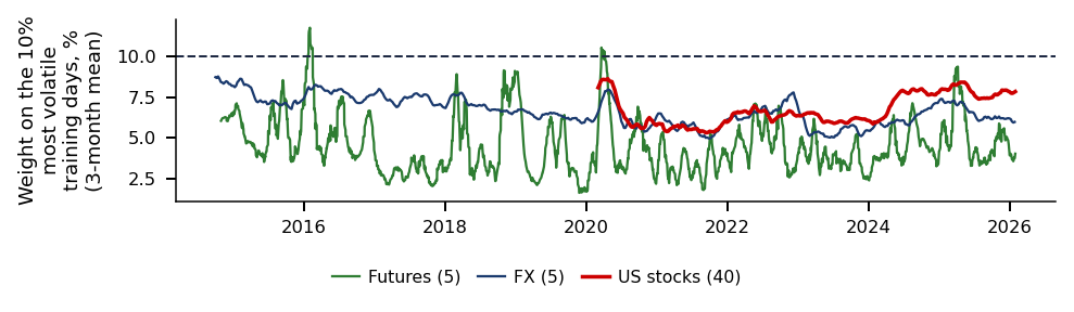
The chart shows the weights that Sig-LK (\(h = 1\)) gives at the origin of 16 March 2020 to the training days, 24 March 2016–13 March 2020, multiplied by the window length so that 1 means equal weighting. The weights are nearly equal, between 0.61 and 1.43 times \(1/n\), and the effective sample size is 975 of 1,000 observations on average over the 40 stocks.
In brief
Weights of Sig-LK (\(h = 1\)) at the origin 16 March 2020 over the training days
training days: 24 Mar 2016 – 13 Mar 2020
weights times the window length: 1 = equal weighting
Nearly equal: between 0.61 and 1.43 times \(1/n\)
effective sample size 975 of 1000 (average over the 40 stocks)
The highest weights go to the last days before the origin. Recent 22-day windows overlap the current window, so their similarity may partly reflect the overlap rather than a distinct economic regime. The late-2018 sell-off receives less weight, not more, and the weights are almost uncorrelated with log volatility (correlation +0.04).
The reason is the translation invariance of the signature: it describes the shape of the path, not its level. A past crisis at a different volatility level does not look similar to the current one, so the kernel cannot implement "learn from past crises".
In brief
The highest weights go to the last days before the origin
Recent 22-point windows overlap the current window
similarity may partly reflect overlap, not a distinct economic regime
The late-2018 sell-off gets less weight
weights are almost uncorrelated with log volatility (+0.04)
the translation-invariant signature sees shape, not level
Sig-LK does not beat log-HAR: at one day the two are close and at a week and a month the signature model loses clearly. The pooled tests confirm only the gain of the log transform over HAR, the apparent Sig-L gain at one day does not survive the balanced panel or the correction over horizons, and in the COVID-19 crash the kernel weights stay almost flat.
Ablations and Robustness
A null result for the full method leaves open which of its two ingredients failed. The ablation crosses the features (signature or not) with the weights (kernel or equal), and the results by asset class show where any gain is concentrated.
Question for the room At h = 1, the mean QLIKE ratio Sig-LK/log-HAR over the 50 assets is 1.045, and the largest ratio is that of crude oil (CL). If we leave CL out, does the mean fall below 1?
Answer
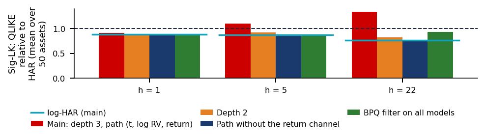
No: the mean falls from 1.045 to 1.011, so leaving CL out does not reverse the descriptive ranking. CL has a ratio of 2.71, but the effect of leaving it out also depends on the other 49 ratios. The weights alone (log-HAR-K) give 1.002, 1.002 and 1.004 relative to log-HAR at h = 1, 5 and 22; Sig-L gives 1.004, 1.285 and 2.238; Sig-LK, 1.045, 1.280 and 1.929. Sig-L evaluates the procedure with signatures and LASSO selection, so its difference from log-HAR cannot be attributed to the features alone.
The question is which ingredient drives the result, the signature features or the kernel weights. The chart reports the mean over the 50 assets of each model's QLIKE loss relative to log-HAR, for the four combinations of features (signature or log-HAR terms only) and weights (kernel or equal). The dashed line marks 1, the loss of log-HAR, so a bar above it means a worse forecast than log-HAR.
In brief
Question: which ingredient drives the result, the signature features or the kernel weights?
Mean over the 50 assets of QLIKE relative to log-HAR
features (signature or not) crossed with weights (kernel or equal)
The dashed line marks 1 (log-HAR)
a bar above it means a worse forecast than log-HAR
The weights alone, log-HAR-K, give ratios of 1.002, 1.002 and 1.004 at \(h = 1\), 5 and 22: no detectable effect on the mean loss. The features alone, Sig-L, give 1.004, 1.285 and 2.238, and both together, Sig-LK, 1.045, 1.280 and 1.929. The average effective sample size with the Sig-LK weights is 816 of 1,000 observations.
Adding the weights to Sig-L reduces the loss at \(h = 22\) without removing it. At \(h = 1\) they make it worse, mainly through crude oil (CL), with a ratio of 2.71, unlike the kernel gain reported in Table 3 of Gu et al. (2024). The loss of the signature models at longer horizons therefore comes from the features, not from the weights.
In brief
Weights alone (log-HAR-K): 1.002, 1.002, 1.004 at \(h = 1, 5, 22\): no detectable effect on the mean loss
Features alone (Sig-L): 1.004, 1.285, 2.238: level-3 terms explode in crashes (Further Topics)
Both (Sig-LK): 1.045, 1.280, 1.929
Average effective sample size with the Sig-LK weights: 816 of 1000
Adding the weights to Sig-L reduces the loss at \(h = 22\) without removing it
They worsen \(h = 1\) through crude oil (CL: 2.71), unlike the kernel gain in Table 3 of Gu et al.
By asset class, the ratio of Sig-L to log-HAR is 1.009, 1.332 and 2.505 for the 40 stocks at \(h = 1\), 5 and 22, 0.965, 1.084 and 1.206 for the 5 futures, and 0.996, 1.111 and 1.134 for the 5 FX pairs. The only gain is for futures at \(h = 1\), 3.5% in QLIKE, and marginally for FX.
Five futures at one horizon are a candidate for a new, pre-registered study, not a finding of this one. The stocks, 80% of the panel, show no gain, and the mean of the ratios over assets is dominated by them. The DM test on the unbalanced panel, by contrast, mixes classes with periods, because before 2020 it holds only futures and FX.
In brief
Sig-L relative to log-HAR (QLIKE)
\(h = 1\)
\(h = 5\)
\(h = 22\)
Stocks (40)
1.009
1.332
2.505
Futures (5)
0.965
1.084
1.206
FX (5)
0.996
1.111
1.134
The only gain: futures at \(h = 1\) (-3.5%) and, marginally, FX
Five futures and one horizon: a candidate for a new, pre-registered study, not a finding of this one
Stocks, 80% of the panel, show no gain
the mean of the ratios over assets is dominated by the stocks
the DM test on the unbalanced panel, however, mixes classes with periods: before 2020 it holds only futures and FX
Section summary
The kernel weights have no detectable effect on the mean loss, and the signature features cause the losses at the week and month horizons. The one gain, for futures at one day, is too narrow to count as a result of this study.
The study evaluates one design out of many, so its null result is not a null result for signatures in general. The design fixes a window of \(L = 22\) days, depth \(N = 3\), three channels, selection by the Bayesian information criterion (BIC) and a four-point grid for the kernel temperature \(c\). Only the truncated kernel is used, and the external factors that are central in Gu et al. (2024), such as implied volatility or macroeconomic news, are absent.
Two benchmark families lie outside the comparison:
A level-aware kernel would add basepoint augmentation or the level of \(\ln\mathrm{RV}\) to the distance (Seminar 20, C2);
The path could be built from intraday 5-minute returns;
The signature kernel could be computed exactly by the partial differential equation (PDE) method of Salvi et al. (2021);
Log-signatures or bounded (tanh) channels could tame the explosive level-3 terms (Morrill et al., 2020).
Cross-asset paths are another direction, since their Lévy areas measure lead–lag across markets, the subject of the case study below. Finally, the futures gain at \(h = 1\) could be tested on a longer panel with this design fixed in advance.
In brief
A level-aware kernel: basepoint augmentation or the level of \(\ln\RV\) in the distance (Seminar 20, C2)
Signatures of the intraday path (5-minute returns)
Log-signatures and bounded (tanh) channels against explosive level-3 terms Morrill et al. (2020)
Cross-asset paths, where Lévy areas measure lead–lag across markets
Futures at \(h = 1\) on a longer panel, with this design fixed in advance
Case Study: The Signature as a Lead-Lag Metric
The case study uses the signature for a different question: not to forecast one series, but to measure whether one asset moves before another. The Lévy area, a level-2 signature term, is a natural candidate, and the study illustrates it on intraday SPY and Bitcoin data.
The question is whether one asset moves before another and whether the signature of their joint path can measure it. Lead–lag relations show in which market information appears first, a question of price discovery. Bennett, Cucuringu and Reinert (2022, Machine Learning) build a directed network from pairwise lead–lag relations and split it into clusters of leaders and followers, using the 434 New York Stock Exchange (NYSE) stocks with the highest volume and daily returns from 2000 to 2019.
One of the metrics they compare is twice the Lévy area of the path of normalised log prices over \([t-m, t]\):
A positive \(S^{ij}\) means that moves of \(i\) are followed by moves of \(j\) in the same direction. Unlike cross-correlations, (20.20) needs no choice of a maximum lag, but it assumes a positive association: it cannot tell "\(i\) leads with negative association" from "\(j\) leads with positive association".
In brief
Question: does one asset move before another, and can the signature of their joint path measure it?
lead-lag relations show in which market information appears first (price discovery)
The empirical results of the paper come from a metric other than the signature (Sections 5–6 of the published version): the area under the cross-correlation function with distance correlation, with lags of up to 5 days, and the Hermitian random-walk (RW) clustering of the network. The lead–lag clusters are significant in a permutation test that shuffles the order of the days; that permutation destroys both the lagged dependence between assets and the autocorrelation of each asset, so on its own it does not separate them.
In the authors' comparisons the clusters do not match Standard Industrial Classification (SIC) sectors, and their correlations with volume and market capitalisation are small. In Section 6.3, the signal built on the clusters has an annualised Sharpe ratio of 0.62, against 0.40 for the S&P 500 over the same period, both before transaction costs. The next slides illustrate the Lévy area on intraday data; they do not replicate the paper's procedure.
In brief
The empirical results of the paper come from a metric other than the signature (published version, Sections 5–6)
the metric: ccf-auc (area under the cross-correlation function) with distance correlation, with lags of up to 5 days
the network clustering: Hermitian RW (random walk)
The lead-lag clusters are significant in a permutation test that shuffles the order of the days
the permutation destroys both the lagged dependence between assets and the autocorrelation of each asset: on its own, the test does not separate them
In the authors' comparisons the clusters do not match SIC (Standard Industrial Classification) sectors
their correlations with volume and with market capitalisation are small
The paper's numbers (Section 6.3): the signal built on these clusters has an annualised Sharpe ratio of 0.62
the S&P 500 has 0.40 over the same period
both are before transaction costs
The next slides: an illustration of the Lévy area on intraday data, not the paper's procedure
Question for the room Across all 489 days, what is the longest tested window for which the mean Lévy area between SPY and Bitcoin is positive and significant at 5% after the Holm correction for the 20 tests?
Answer
120 minutes: NW (Newey–West, standard errors) t ≈ 3.05 and Holm-adjusted p ≈ 0.032. At 195 minutes, NW t ≈ 2.45 passes the pointwise 1.96 threshold, but the adjusted p is 0.157. The 10-minute option confuses the window with the strongest signal (t = 9.6, the area positive on 70% of the days) with the longest significant window; 195 minutes uses the pointwise threshold instead of the correction. Over the whole session, t = 1.51. The correlation between SPY at t − 1 and BTC (Bitcoin) at t is 0.088 (NW t = 9.8), and in the reverse direction −0.005. The 20 tests (12 lags and 8 windows) are exploratory, and the result indicates a lead-lag association, not causality. The effect weakens in 2026: the lag +1 correlation falls to 0.04.
The data are five-minute bars of SPY, the S&P 500 exchange-traded fund (ETF), and of Bitcoin (BTC, in USD), New York time, 09:30–16:00, on the 489 days with all 78 bars for both assets out of 513 common days, 3 September 2024–18 September 2026. The left panel shows the mean over days of the correlation between the SPY return at \(t-l\) and the BTC return at \(t\), with pointwise 95% intervals from the Newey–West (NW) standard errors. The right panel shows the NW \(t\)-statistic of the mean daily Lévy area of (SPY, BTC) for windows from 10 minutes to the whole session; the line at 1.96 is a pointwise threshold.
In brief
SPY (the S&P 500 ETF; ETF: Exchange-Traded Fund) and Bitcoin (BTC, in USD): five-minute bars, New York time, 09:30–16:00
489 days with all 78 bars for both assets (out of 513 common days), 3 Sep 2024 – 18 Sep 2026
Left: mean over days of the correlation between the SPY return at \(t - l\) and the BTC return at \(t\); bars: pointwise 95% intervals with the Newey-West (NW) standard error of the tests
Right: NW \(t\)-statistic of the mean daily Lévy area (SPY, BTC), for windows from 10 minutes to the whole session; the line at 1.96 is a pointwise threshold
The path of each day is formed by the cumulative sums of the SPY and BTC returns, each return divided by the standard deviation of its asset on that day, as the authors recommend, since otherwise the area grows with volatility. The 78 returns run from the open of the 09:30 bar to the close of each bar from 09:30 to 15:55. The Lévy area of a window of \(m\) steps is a sum of lagged products of the SPY returns \(x_i\) and the BTC returns \(y_i\):
In (20.21) lag \(l\) appears \(m-l\) times, so a window of 2 steps, 10 minutes, keeps lag 1 only, while a long window adds many lags without effect and hence noise. The daily statistic is the mean area over all windows of \(m\) steps in the day, and the test is the NW \(t\) with 8 lags on the 489 daily values (Newey & West, 1987). The illustration differs from the paper: two assets instead of 434, five-minute bars instead of daily returns, and no network clustering or trading signal.
In brief
The path of the day: cumulative sums of the SPY and BTC returns, each return divided by the standard deviation of its asset on that day
78 returns: from the open of the 09:30 bar to the close of each bar 09:30–15:55
the normalisation the authors recommend: otherwise the area grows with volatility
The Lévy area of a window of \(m\) steps is a sum of lagged products of the returns \(x_i\) (SPY) and \(y_i\) (BTC)
SPY moves before Bitcoin by one five-minute step. The correlation at lag +1 is 0.088 (NW \(t\) = 9.8), and at lag −1 it is −0.005 (\(t\) = −0.71); the direct test of direction, the difference between the two, is 0.093 (NW \(t\) = 9.5). The contemporaneous correlation is 0.40, and at lags +2 to +6 the correlations are small and negative, between −0.016 and −0.004.
The signature metric finds the effect only in short windows. With 10-minute windows \(t\) = 9.6 and the area is positive on 70% of the days; with 2-hour windows \(t\) = 3.0; over the whole session of 390 minutes \(t\) = 1.51 and the area is positive on 51% of the days. The analysis is exploratory, with 20 tests (12 non-zero lags and 8 windows): the Holm-adjusted p-value is 0.032 for the 2-hour window and 0.157 for 195 minutes. The effect weakens in 2026: the lag +1 correlation is 0.11 in 2024, 0.12 in 2025 and 0.04 in January–September 2026.
In brief
SPY moves before Bitcoin by one five-minute step
the correlation at lag \(+1\) is 0.088 (NW \(t\) = 9.8), and at lag \(-1\) it is \(-\)0.005 (\(t\) = \(-\)0.71)
the direct test of direction: the difference between the correlations at lags \(+1\) and \(-1\) is 0.093 (NW \(t\) = 9.5)
the contemporaneous correlation is 0.40; at lags \(+2\) to \(+6\) the correlations are small and negative (between \(-\)0.016 and \(-\)0.004)
The signature metric finds the effect only in short windows
10 minutes: \(t\) = 9.6, and the area is positive on 70% of the days
2 hours: \(t\) = 3.0; the whole session (390 minutes): \(t\) = 1.51, area positive on 51% of the days
The analysis is exploratory: 20 tests (12 non-zero lags and 8 windows)
Holm-adjusted \(p\): 0.032 for the 2-hour window, 0.157 for 195 minutes
The effect weakens in 2026: the lag \(+1\) correlation is 0.11 in 2024, 0.12 in 2025 and 0.04 in 2026 (January–September)
The result supports a five-minute lead–lag association between two assets, not a causal relation and not a profitable signal, since there are no trading costs and no out-of-sample evaluation. The sign of the area measures the orientation of the path, and reading it as "SPY leads" assumes a positive association between the two assets.
Three limits remain:
A one-step lag also arises from unsynchronised timestamps of the two data sources, and separating the two explanations needs tick data.
The window length \(m\) plays the role of the maximum lag, so the signature does not remove this choice.
The NW \(t\)-test needs finite moments and weak dependence of the daily statistic tested, bounded correlations and normalised areas, not of the raw returns.
In brief
Type of evidence: a five-minute lead-lag association between two assets, not a causal relation and not a profitable signal
no trading costs and no out-of-sample evaluation
The sign of the area measures the orientation of the path; reading it as “SPY leads” assumes a positive association between the two assets
Limits
a one-step lag also arises from unsynchronised timestamps of the two sources; separating the two needs tick data
the window length \(m\) plays the role of the maximum lag: the signature does not remove this choice
the NW \(t\)-test needs finite moments and weak dependence of the daily statistic tested (bounded correlations, normalised areas), not of the raw returns
Section summary
The Lévy area detects the five-minute lead of SPY over Bitcoin only when the window is short, because longer windows add lags that carry no signal. The window length acts as the maximum lag of a correlation analysis, and the association is not a trading result.
AI for Scientific Discovery
The chapter is itself a transfer study: a method from a data-mining conference paper applied to a financial forecasting problem. The section turns this into a general question, states the criterion for a successful transfer and shows how the AI-assisted (Artificial Intelligence) loop was applied and where it can mislead.
Methods travel faster than evidence: a Knowledge Discovery and Data Mining (KDD) conference paper on freight rates becomes a candidate for volatility, credit or energy. Two questions decide whether a transfer can work:
Which properties of the source problem made the method work;
Whether the target shares them.
Finance adds a hard filter: in Menkveld et al. (2024), 164 teams working on the same data disagree more than their standard errors suggest.
The criterion is that a transfer succeeds if the gain over the strongest simple benchmark survives across a pre-registered set \(\mathcal{S}\) of designs, assets and horizons, with the family corrected. In this chapter \(\mathcal{S}\) is 50 assets by 3 horizons by 4 variants. Holm and BH were applied per comparison and horizon, to families of 50 assets, and the variants are reported descriptively, without a joint correction over all 600 cells.
In brief
Methods travel faster than evidence
a KDD paper on freight rates becomes a candidate for volatility, credit, energy
Which properties of the source problem made the method work?
164 teams on the same data disagree more than their standard errors suggest
Criterion: a transfer succeeds if the gain over the strongest simple benchmark survives
a pre-registered set \(\mathcal{S}\) of designs, assets and horizons
with the family corrected
In this chapter: \(\mathcal{S}\) = 50 assets \(\times\) 3 horizons \(\times\) 4 variants; Holm/BH were applied per comparison and horizon (families of 50 assets), variants reported descriptively; no joint correction over all 600 cells
In the reading step an assistant lists every equation, hyperparameter and benchmark of the paper and marks what is not disclosed, and each item is checked against the PDF.
The mapping step decides, for each component, whether it transfers, what must change and which benchmark isolates it.
The pre-registration fixes the hypotheses, grid, tests and correction in a dated document before the first result; the assistant drafts, the team decides every number.
The pieces are built and tested: signatures are checked against identities, such as level 1 equal to the increment and Chen's identity on a split path, not against another library.
The grid is run and then attacked, with Holm over 50 assets and a search for the single asset that would make a misleading headline.
The null is explained with data (checklist in the Appendix): here, flat weights caused by translation invariance and explosive level-3 terms caused by the exponential link.
In brief
Read: an assistant lists every equation, hyperparameter and benchmark of the paper
Three headlines can be written from the same runs:
"Signatures beat HAR on 12 of 50 assets" (one-day horizon, raw DM) is true, but log-HAR alone beats HAR on 21, so the gain belongs to the log transform.
"Signatures improve E-mini S&P 500 volatility forecasts" (ES, \(h = 1\), DM \(t = -2.91\) against log-HAR) rests on one cell out of 150 asset-horizon cells; after Holm, 0 of 50 assets are significant at \(h = 1\) and none at \(h = 5\) or 22.
The headline of the pre-registered evaluation: "no robust advantage over log-HAR in the specification evaluated; worse at longer horizons; no detectable effect of the kernel weights".
An AI assistant asked to "find where the method works" will produce the first two headlines; the plan protects the third. The result supports a comparison of procedures: the same runs read without correction, on a single cell, or by the pre-registered plan.
In brief
“Signatures beat HAR on 12 of 50 assets” (Sig-LK, one-day horizon, raw DM)
True, but log-HAR alone beats HAR on 21: the gain belongs to the log transform
“Signatures improve E-mini S&P 500 volatility forecasts” (ES, \(h = 1\), DM \(t = -2.91\) for Sig-LK against log-HAR)
One cell out of 150 asset-horizon cells: after Holm, Sig-LK wins on 0 of 50 at \(h = 1\) and none at \(h = 5, 22\)
The headline of the pre-registered evaluation
“no robust advantage over log-HAR in the specification evaluated; worse at longer horizons; no detectable effect of the kernel weights”
An AI (Artificial Intelligence) assistant asked to “find where the method works” will produce the first two; the plan protects the third
Type of evidence: comparison of procedures
the same runs, read without correction, on a single cell or by the pre-registered plan
The project picks one open direction of the chapter, such as a level-aware kernel, intraday signatures, log-signatures or futures only, and writes \(H_0\) and \(H_1\), the benchmark that isolates the idea and the result that would lead to dropping it. An assistant lists what could go wrong in the design, and each item gets one unit test.
The pre-registration is fixed in a dated document before the first out-of-sample number; then the grid is run and the distribution of results over \(\mathcal{S}\) is reported. Every AI error caught goes into `AI_ERRORS.md`; Seminar 20, C1, gives typical ones.
In brief
Pick one open direction of this chapter
level-aware kernel, intraday signatures, log-signatures, futures only
Write \(H_0\)/\(H_1\), the benchmark that isolates it, and the result that would make you drop it
Use an assistant to list what could go wrong in your design, then write one unit test per item
Fix the pre-registration in a dated document before the first out-of-sample number
run the grid
report the distribution over \(\mathcal{S}\)
Log every AI error you catch in AI_ERRORS.md (Seminar 20, C1 gives typical ones)
Signatures turn a window into a feature vector with a theory behind it: Chen's identity, uniqueness and universality. Transferred to realised variance, the method of Gu et al. (2024) does not beat log-HAR:
H1, that signatures add information, is not supported, with no gain at one day and a loss at a week and a month.
H2, that kernel weights help, is not supported: the weights are almost flat and down-weight past stress.
H3 holds only against HAR in levels, through the log target.
H4, gains in stress, is not supported.
Two mechanisms explain the null: the translation-invariant kernel sees shape, not level, and the level-3 terms explode in crashes. The strongest effect in the study is the oldest one, modelling the log of RV. The null result is informative, because the ablations and the mechanism explain why the method does not transfer.
In brief
Signatures turn a window into a feature vector with a theory behind it
Chen’s identity; uniqueness and universality (details in Further Topics)
Transferred to realised variance, the method of Gu et al. does not beat log-HAR
H1 (signatures add information): not supported, no gain at one day, a loss at a week and a month
H2 (kernel weights help): not supported, weights are almost flat and down-weight past stress; H3: only HAR in levels is beaten, through the log target; H4 (gains in stress): not supported
The translation-invariant kernel sees shape, not level
level-3 terms explode in crashes
The strongest effect in the study is the oldest one: model the log of RV
The null result is informative
the ablations and the mechanism explain why the method does not transfer
The chapter chooses log-HAR to forecast daily realised variance; the method of Gu et al. (2024), Sig-LK, does not replace it. log-HAR is in the 90% MCS for 100%, 98% and 98% of the assets at \(h = 1\), 5 and 22, and on the panel it beats HAR at every horizon, with DM \(t\) from −3.09 to −4.50.
The choice holds under three conditions:
QLIKE as the main loss, with the log target and the variance correction \(\hat s^2/2\);
Rolling estimation, re-estimated every 5 days on the last 1,000 pairs;
A panel dominated by stocks, 40 of the 50 assets.
It would be dropped if a gain of Sig-L or Sig-LK over log-HAR survived the Holm correction in a pre-registered study, for example the Sig-L gain on futures at \(h = 1\), −3.5% in QLIKE, confirmed on a longer panel.
In brief
What I choose: log-HAR to forecast daily realised variance; the method of Gu et al. (Sig-LK) does not replace it
log-HAR is in the 90% MCS for 100%, 98% and 98% of the assets at \(h = 1\), 5 and 22
on the panel, log-HAR beats HAR at every horizon (DM \(t\) from \(-3.09\) to \(-4.50\))
Under which conditions
QLIKE as the main loss, with the log target and the variance correction \(\hat s^2/2\)
rolling estimation, re-estimated every 5 days on the last 1000 pairs
a panel dominated by stocks (40 of the 50 assets)
What result would make me drop it
a gain of Sig-L or Sig-LK over log-HAR that survives the Holm correction in a pre-registered study
for example, the Sig-L gain on futures at \(h = 1\) (\(-3.5\%\) in QLIKE), confirmed on a longer panel
Further Topics
The Further Topics give the data background, the two refinements of HAR, the theory of signatures and details of the evaluation. They are reading for familiarity.
Why Five-Minute RV, and Where Do the Data Come From?
Alternatives to five-minute realised variance (RV) include bipower variation, robust to jumps, the realised kernel, robust to noise (Barndorff-Nielsen et al., 2008), and range-based estimators, but across 400 assets little beats five-minute RV as a proxy of daily variance (Liu, Patton & Sheppard, 2015). Its semivariances and quarticity are computed on the same grid, so SHAR and HARQ use consistent inputs, and every model is evaluated on the same target. VOLARE is built at the Universities of Messina and Florence from tick data with the same estimators for every asset class (Cipollini et al., 2026); it is free for research at volare.unime.it and is not redistributed with the course.
RV measures the integrated variance with error, \(\mathrm{RV}_t = \mathrm{IV}_t + \eta_t\) with \(\mathrm{Var}(\eta_t) \approx 2\,\mathrm{IQ}_t/M\), and errors in variables pull the daily coefficient \(\beta_d\) towards zero, most on noisy days. HARQ (Bollerslev, Patton & Quaedvlieg, 2016) lets the weight on yesterday's RV depend on the square root of realised quarticity:
with \(\beta_Q < 0\) expected, so that a noisy day gets less weight. The BPQ "insanity filter" replaces a forecast outside the in-sample range of the target by the in-sample mean.
\(\mathrm{RQ}_t^{1/2}\): square root of realised quarticity, a measure of the error of \(\RV_t\); \(\overline{\mathrm{RQ}^{1/2}}\): its in-sample mean, so \(\beta_d\) is the weight on an average day
Expected \(\beta_Q < 0\): on a noisy day (\(\mathrm{RQ}_t\) above average) yesterday’s RV gets less weight
SHAR (Patton & Sheppard, 2015) splits the daily term by the sign of the intraday returns, \(\mathrm{RV}_{t+1:t+h} = \beta_0 + \beta^{+}\mathrm{RV}_t^{+} + \beta^{-}\mathrm{RV}_t^{-} + \beta_w\mathrm{RV}_t^{(w)} + \beta_m\mathrm{RV}_t^{(m)} + \varepsilon_{t+h}\), where \(\mathrm{RV}_t^{+}\) and \(\mathrm{RV}_t^{-}\) are the positive and negative semivariances; \(\beta^{+} = \beta^{-}\) gives back HAR. Patton and Sheppard find \(\beta^{-} > \beta^{+}\), an intraday version of the leverage effect (Chapter 5), and the signature can capture a related effect from daily data through the Lévy area between returns and log RV.
The chart draws two 22-day windows of JPM as paths in the plane of cumulative open-to-close return and log RV, with the chord from start to end and the shaded Lévy area. In the calm window to 15 November 2019 log RV moves by −0.58 and the Lévy area is −0.011; in the stress window to 16 March 2020 log RV rises by +4.32, RV multiplied by 75, while the intraday return path falls and recovers, and the Lévy area is −0.247.
In brief
Path (cumulative open-to-close return, log RV) over 22 days
dashed chord from start to end
the shaded region gives the Lévy area
Calm window (to 15 Nov 2019) vs stress window (to 16 Mar 2020)
calm: log RV moves by -0.58, the path wanders, Lévy area -0.011
stress: log RV rises by +4.32 (RV \(\times\) 75) while the intraday return path falls and then recovers
stress: Lévy area -0.247 (returns in decimal units for the area, percent on the axis)
The net intraday return of the stress window is only +0.5%, because the crash happened largely overnight, outside the open-to-close channel. No signature level recovers what the input omits.
In brief
The net intraday return is only +0.5%
the crash was largely overnight, outside this channel
By the uniqueness theorem of Hambly & Lyons (2010), the full signature determines the path up to tree-like equivalence and translation, and with a strictly increasing time channel only translation remains; a finite truncation is not injective. The shuffle identity, for example \(S^iS^j = S^{ij} + S^{ji}\), writes products of signature terms as sums of higher terms, so a linear model in the truncated signature already contains polynomials of the increments.
Universality states that any continuous function of the path on a compact set \(K\) of time-augmented paths is approximated uniformly by a linear functional \(\langle \ell, \mathrm{Sig}(X)\rangle\) of the signature, a consequence of the Stone–Weierstrass theorem through the shuffle identity. This allows nonlinear approximation at sufficient depth but guarantees nothing at depth 3 or out of sample. Factorial decay, \(\|S^{(k)}\| \le \|X\|_{1\text{-var}}^k/k!\), makes the high levels small for paths of moderate length.
In brief
Universality: any continuous function of the path is approximately linear in the signature
\(K\): a compact set of time-augmented paths with a common start (in the 1-variation topology); \(f: K \to \mathbb{R}\): a continuous function of the path
\(\langle \ell, \Sig(X)\rangle\): a weighted sum of finitely many signature terms, i.e. a linear regression on them
Sufficient depth permits nonlinear approximation; this does not guarantee accuracy at depth 3 or out of sample. The cost is \(d^N\) features, so sparsity is needed
terms. With \(d = 3\) channels (time, log RV, cumulative return) and \(N = 3\) this gives \(3 + 9 + 27 = 39\) terms, of which 3 are constant and 36 vary; \(d = 5\) and \(N = 4\) would give 780 terms for 1,000 observations, too many for a stable LASSO selection. \(N = 3\) and \(L = 22\) are fixed in advance, with \(N = 2\) as a robustness check.
In brief
Number of terms in levels \(1..N\) of a \(d\)-dimensional path (a geometric sum, since level \(k\) has \(d^k\) words)
The signature is translation invariant, \(\mathrm{Sig}(X + c) = \mathrm{Sig}(X)\), so the level of volatility enters separately through the log-HAR terms, which play the role of the external factors of Gu et al. (2024). Basepoint augmentation (Morrill et al., 2020) prepends the origin to the path, which makes the higher-order terms depend on the absolute level and the signature level-aware; translating the path to start at 0 does not, because it is itself a translation. Without a time channel the signature is also invariant to reparametrisation, so the same move run at different speeds has the same signature.
In brief
Translation invariance: \(\Sig(X + v) = \Sig(X)\) for any constant vector \(v \in \mathbb{R}^d\)
only increments enter
The signature does not see the level of volatility, so the level enters separately: the log-HAR terms play the role of the external factors \(x_\tau\) of Gu et al.
Basepoint augmentationMorrill et al. (2020): the path starts at the origin, then runs through the points of the window
Level 1 becomes \(X_{u_0} + (X_{u_{L-1}} - X_{u_0}) = X_{u_{L-1}}\): the starting point does not appear on its own, but the higher-order terms depend on the absolute level (for example \(\ln\RV\)), so the signature becomes level-aware
Translating the path to start at 0 does not do this: it is itself a translation (Seminar 20, C2 uses the prepended segment)
Reparametrisation invariance: \(X_{\psi(u)}\), with \(\psi\) increasing, has the same signature
without a time channel, two moves with the same spatial shape, run at different speeds, have the same signature
the time channel tells them apart by referring them to a fixed clock; the augmented path stays invariant to a reparametrisation of the whole augmented path
\(u_i = i/(L-1)\) maps every window to \([0, 1]\): the absolute duration (22 vs 2 days) needs physical time or a separate regressor
In this chapter: time augmentation, no basepoint
so the kernel compares shapes, not levels
the consequence shows in the kernel weights (Results section)
With three windows at distances \(\delta = (0.1, 0.4, 0.9)\) and \(\gamma = 2\), the unnormalised weights are \((0.819, 0.449, 0.165)\), with sum 1.433, and the normalised weights \(w = (0.571, 0.313, 0.115)\). The effective sample size \(n_{\mathrm{eff}} = 1/\sum w_i^2 \approx 2.28\), against 3 under equal weights; \(\gamma\) acts as an inverse temperature, so a larger \(\gamma\) concentrates the weights, gaining similarity and losing information.
In brief
Distances \(\delta=(0.1, 0.4, 0.9)\) and \(\gamma=2\)
Unnormalised weights: \((0.819, 0.449, 0.165)\), with sum \(1.433\)
Normalised weights: \(w=(0.571, 0.313, 0.115)\)
\(n_{\mathrm{eff}}=1/\sum w_i^2\approx2.28\), compared with 3 under equal weights
\(\gamma\) acts as an inverse temperature
a larger \(\gamma\) concentrates the weights, gaining similarity and losing information
The loss differential \(d_t\) is autocorrelated, through overlapping targets up to lag \(h - 1\) and volatility clustering in the losses, so the plain variance understates the uncertainty of \(\bar d\). The Newey–West heteroskedasticity and autocorrelation consistent (HAC) estimator (Newey & West, 1987) is
with \(\hat\gamma_j\) the sample autocovariance of \(d_t\) at lag \(j\); the Bartlett weights guarantee \(\hat\Omega \ge 0\), and \(q = \max(h, \lceil T^{1/3}\rceil)\) lags cover at least the overlap.
In brief
Why not the plain sample variance: \(d_t\) is autocorrelated
overlapping targets up to lag \(h - 1\)
volatility clustering in the losses
so \(\hat\Gamma_0/T\) understates the uncertainty of \(\bar d\) (and over-rejects) when the sum of the autocovariances is positive, the typical case with overlapping targets
The Newey–West estimator Newey & West (1987), heteroskedasticity and autocorrelation consistent (HAC)
Holm compares three sorted p-values, \((0.004, 0.023, 0.08)\), in turn with \((0.05/3, 0.05/2, 0.05)\): the first two pass, the third fails, and the procedure stops. BH compares them with \((0.05/3, 2\cdot0.05/3, 0.05)\) and keeps the largest passing rank, again two; in a family of 50 tests the same p-values may no longer pass. For an MCS with models A, B and C and standardised loss gaps 2.4, −0.5 and −0.7, the bootstrap p-value 0.04 removes A at 10%, the retest of B and C gives 0.30, and both remain, which does not prove that their population losses are equal.
In brief
Holm compares three sorted p-values, \((0.004, 0.023, 0.08)\), in turn with \((0.05/3, 0.05/2, 0.05)\)
the first two pass, the third fails, so we stop
BH compares them with \((0.05/3, 2 \cdot 0.05/3, 0.05)\) and keeps the largest passing rank: again two
In a family of 50 tests the same p-values may no longer pass
which is why the family is fixed before the results
MCS with three models A, B and C, standardised loss gaps 2.4, \(-0.5\) and \(-0.7\)
the bootstrap p-value is 0.04, so at 10% we remove A
Recompute the test for B and C only: the new p-value is 0.30, so we stop and B and C remain
Failure to separate them is not proof that their population losses are equal
The 90% coverage is a repeated-sample guarantee, not a posterior probability for the set obtained
The heat map gives the DM \(t\)-statistics of the QLIKE differential of Sig-LK for each of the 40 stocks, 5 futures and 5 FX pairs, blue where Sig-LK is more accurate and red where it is less. Against log-HAR the map is pale at \(h = 1\) and red at \(h = 5\) and 22, with blue exceptions for ES, Tesla (TSLA) and EURUSD and five assets significantly red before correction; against HAR it is blue at \(h = 1\), because Sig-LK inherits the log target.
In brief
Diebold–Mariano \(t\)-statistics of the QLIKE differential, one column per asset ticker
40 stocks, 5 futures, 5 FX pairs
blue: Sig-LK more accurate, red: less accurate
Against log-HAR (top): pale at \(h = 1\), red at \(h = 5, 22\)
blue exceptions: ES, TSLA = Tesla, EURUSD
five assets significantly red before correction
Against HAR (bottom): blue at \(h = 1\) because Sig-LK inherits the log target
The chart shows the weight that Sig-LK (\(h = 1\)) puts on the 10% most volatile days of its training window, averaged by class over three months. For stocks the mean is 6.7% per re-estimation, below the 10% of equal weighting, ranging from 4.4% to 9.9% (maximum on 17 March 2020); FX stays below 10% throughout, and futures exceed it only in early 2016 (up to 11.7%) and in March–April 2020.
In brief
Weight that Sig-LK (\(h = 1\)) puts on the 10% most volatile days of its training window
averaged by class, three-month mean
Stocks, per re-estimation: mean 6.7%, below the 10% of equal weighting
between 4.4% and 9.9% (maximum on 17 Mar 2020)
FX stays below 10% throughout
Futures exceed 10% (three-month mean) only in two short episodes
Across all assets and horizons, the LASSO, with its support selected by BIC, keeps the three log-HAR terms in 99%, 94% and 93% of the re-estimations, so it rediscovers HAR. The average support has 8.7 regressors for Sig-L and 6.7 for Sig-LK. The most frequent signature term, (t, r, r), selected in 27% of the re-estimations, and all the frequent ones are of level 3, cubic in the increments.
In brief
Across all assets and horizons: share of re-estimations in which a regressor is in the support of Sig-LK
the support is selected by BIC
labels: HAR day/week/month = the three log-HAR terms, t = time, ln RV = \(\ln\RV\), r = cumulative return
The log-HAR terms are kept in 99%, 94% and 93% of the re-estimations
the LASSO rediscovers HAR
average support 8.7 regressors (Sig-L), 6.7 (Sig-LK)
The most frequent signature term, (t,r,r) (27%), and all frequent ones are of level 3
cubic in the increments
far outside the training range in a crash, amplified by \(\exp(\cdot)\)
The chart compares Sig-LK relative to HAR, as a mean over the 50 assets, in the main design, in two pre-registered variants and with the BPQ filter; the reference line marks log-HAR, and a bar below 1 means a more accurate forecast than HAR.
In brief
Sig-LK relative to HAR (mean over 50 assets)
in the main design and in two pre-registered variants
with the BPQ filter (the disclosed deviation)
The reference line marks log-HAR
a bar below 1 means a more accurate forecast than HAR
At depth 2 the ratios at \(h = 5\) and 22 fall from 1.104 and 1.334 in the main design to 0.922 and 0.820, and without the return channel to 0.878 and 0.770, close to log-HAR (0.871 and 0.765). The ablations suggest that the long-horizon failures are linked to level-3 terms that contain the return channel, although removing terms also changes the selection, the kernel distances and the weights. Both variants reduce the instability; neither establishes H1.
In brief
Depth 2: 0.922 and 0.820 at \(h = 5, 22\) (main design: 1.104, 1.334)
Path without returns: 0.878 and 0.770
the ablations suggest that the long-horizon failures are linked to terms that contain the return channel
Depth 2 also reduces them: the ablations suggest a role of the level-3 terms
removing terms, however, also changes the selection, the kernel distances and the weights
Without returns the model approaches log-HAR (0.871 and 0.765)
The Appendix gives the details of the features, the estimation, the evaluation windows and the chosen temperatures, the paper's own error metric on VOLARE, the filtered results, the researcher's checklist and the prompts of the discovery loop.
The regressors at day \(\tau\) are the three log-HAR terms and the 39 terms of the depth-3 signature of the 22-point path (time, \(\ln\mathrm{RV}\), cumulative return). Each non-time channel \(q\) is multiplied by \(\kappa_q = 1/(s_q\sqrt{L-1})\), with \(s_q\) the standard deviation of its daily increments in the training window, so its typical total move over the window is about 1; time runs from 0 to 1, a word is rescaled by the product of its factors, every column is standardised with weighted moments and constant columns are dropped.
Inside each training window the whole weighted LASSO path is computed by least-angle regression (LARS), each support on the path is refitted by weighted OLS (step 2 of Gu et al. (2024)), and the support minimising
is chosen, with \(\hat s^2_S\) the weighted residual variance. Cross-validation would be too costly over 50 assets, 3 horizons and hundreds of re-estimations; the Kish size \(n_{\mathrm{eff}}\) corrects for unequal weights but not for serial dependence, so (20.25) is a heuristic of the design, not a likelihood-based BIC.
In brief
Inside each training window: the whole weighted LASSO path by LARS
For every support on the path: weighted OLS refit (step 2 of Gu et al.)
Pick the support that minimises a BIC-type criterion with the Kish effective sample size
\(S\): a support (set of kept regressors), \(|S|\): its size, \(+1\) for the intercept; \(\hat s^2_S\): weighted residual variance of the refit on \(S\)
Why not cross-validation: 50 assets \(\times\) 3 horizons \(\times\) hundreds of re-estimations
BIC uses only the window
Kish size corrects for unequal weights, not for serial dependence (overlapping targets, \(h > 1\)): not a likelihood-based BIC for these data
Evaluation starts on 27 January 2020 for stocks, 25 September 2014 for futures and 27 August 2014 for FX, and ends on 29 January 2026, with median lengths of 1,499, 2,919 and 2,952 days per asset. Each model produces 265,929 forecasts over the three horizons: 89,893 at \(h = 1\), 89,293 at \(h = 5\) and 86,743 at \(h = 22\). Because the stock data start in 2015, the COVID-19 crash is in every stock evaluation sample.
In brief
Class
Evaluation starts
Ends
Days per asset (median)
Stocks
27 Jan 2020
29 Jan 2026
1 499
Futures
25 Sep 2014
29 Jan 2026
2 919
FX
27 Aug 2014
29 Jan 2026
2 952
265 929 forecasts per model over the three horizons: 89 893 (\(h = 1\)), 89 293 (\(h = 5\)), 86 743 (\(h = 22\))
Stocks start in 2015, so their evaluation begins in January 2020
the COVID-19 crash is in every stock sample
Futures and FX start in 2009 and are evaluated from 2014
The kernel temperature \(c\) is chosen from the grid {0.5, 1, 2, 4} on the validation block of each class and horizon. For Sig-LK it is 0.5 for stocks at all horizons, 2.0, 1.0 and 0.5 for futures, and 0.5, 2.0 and 0.5 for FX; log-HAR-K uses the largest value, 4.0, for futures at \(h = 22\) and for FX at \(h = 1\) and 22.
In brief
Sig-LK
log-HAR-K
Class
\(h = 1\)
\(h = 5\)
\(h = 22\)
\(h = 1\)
\(h = 5\)
\(h = 22\)
Stocks
0.5
0.5
0.5
0.5
0.5
1.0
Futures
2.0
1.0
0.5
2.0
1.0
4.0
FX
0.5
2.0
0.5
4.0
2.0
4.0
The value of \(c\) from the grid \(\{0.5, 1, 2, 4\}\), chosen on the validation block of each class and horizon
On the paper's own metric, the median over assets of the mean relative error \(|\mathrm{RV} - F|/\mathrm{RV}\), log-HAR has 50.4%, 41.9% and 38.7% at \(h = 1\), 5 and 22, against 57.2%, 48.9% and 51.7% for HAR, 50.1%, 42.6% and 42.6% for Sig-L and 50.6%, 43.6% and 43.7% for Sig-LK.
In brief
Median of asset mean errors \(|\RV - F|/\RV\) (%)
\(h = 1\)
\(h = 5\)
\(h = 22\)
HAR
57.2
48.9
51.7
log-HAR
50.4
41.9
38.7
HARQ
55.0
49.0
50.7
SHAR
57.9
49.2
51.8
log-HAR-K
49.7
41.0
38.7
Sig-L
50.1
42.6
42.6
Sig-LK
50.6
43.6
43.7
Median over assets of the mean relative error: about 40–60%
against 1–2% for freight rates in Gu et al.
Daily RV is a noisy, heavy-tailed target
the evaluated models have much larger relative errors than those reported for freight rates
this does not establish a lower bound on attainable error
Sig-LK forecasts above ten times the in-sample maximum: 8 at \(h = 1\), 29 at \(h = 5\) (concentrated on 10 assets) and 36 at \(h = 22\); log-HAR: none
With the BPQ filter applied to all models, the QLIKE ratios to HAR at \(h = 1\), 5 and 22 are 0.763, 0.654 and 0.778 for log-HAR, 0.995, 0.912 and 1.014 for HARQ, 0.871, 0.819 and 0.904 for Sig-L and 0.890, 0.867 and 0.930 for Sig-LK. The filter rescues HARQ, but log-HAR keeps the lowest loss at every horizon.
In brief
QLIKE relative to HAR, BPQ filter on all models
\(h = 1\)
\(h = 5\)
\(h = 22\)
HAR
1.000
1.000
1.000
log-HAR
0.763
0.654
0.778
HARQ
0.995
0.912
1.014
SHAR
1.014
1.003
1.000
log-HAR-K
0.772
0.659
0.779
Sig-L
0.871
0.819
0.904
Sig-LK
0.890
0.867
0.930
The filter rescues HARQ relative to HAR (0.995 at \(h = 1\) instead of 1.140), as BPQ intended
Sig-LK relative to log-HAR, both filtered: 1.238, 1.424, 1.209
the gap widens at \(h = 1, 5\) and narrows at \(h = 22\)
The method must be the paper's, with each component pointing to the equation, table or section it comes from and undisclosed choices labelled as choices of the study.
There must be no look-ahead: changing every value after the origin, for example multiplying future RV by 10, must leave the forecast unchanged.
The benchmark must isolate the idea, through the 2 × 2 ablation.
The losses and tests must be the right way round, with \(\mathrm{QL}(\mathrm{RV}, \mathrm{RV}) = 0\) and a HAC variance with bandwidth at least \(h\).
In brief
The method is the paper’s: kernel, weights, refit, as in the cited equations
Test: each component of the method points to the equation, table or section of the paper it comes from; undisclosed choices are labelled as choices of the study
No look-ahead: \(\lambda\), scales, \(c\) and features use only data available at the origin
Test: change every value after the origin (for example, multiply future RV by 10); the forecast made at the origin must not change
The benchmark isolates the idea: the \(2 \times 2\) ablation is reported, not only the full model against HAR
Losses and tests are the right way round: \(\QL(\RV, \RV) = 0\) and \(\QL(\RV, F) > 0\) otherwise
The DM variance is HAC with bandwidth at least \(h\)
The reading prompt asks the assistant to list every equation of the estimator of Gu et al. (2024), every hyperparameter with its reported value and the benchmark of each table, marking what is not disclosed, and each item is checked against the PDF. The mapping prompt asks, for daily realised variance, whether each component transfers, what must change and which benchmark isolates it; the pre-registration is then fixed in a dated document signed by the team before the first result.
In brief
Read: extract exactly what the paper did
“From Gu et al. (2024, KDD), list every equation of the estimator, every hyperparameter and its reported value, and the benchmark of each table. Mark what is not disclosed.”
Check each item against the PDF: equation numbers, table numbers, the kernel actually used
Map: what transfers, what must be adapted
“Our target is daily realised variance. For each component of the method, say whether it transfers, what must change, and which benchmark isolates it.”
Pre-register: hypotheses, grid, tests, correction
fixed in a dated document signed by the team before the first result
The testing prompt asks for unit tests of a depth-3 signature: level 1 equal to the increment, the symmetric part of level 2 equal to half the outer product, and Chen's identity on a split path. The attack prompt gives all 600 runs, 50 assets by 3 horizons by 4 specifications, and asks which conclusions survive Holm over 50 assets and which single asset or subperiod would make a misleading headline; the last step explains the null by its mechanism, not by an excuse.
In brief
Build and test the pieces: signatures against identities, not against another library
“Write unit tests for a depth-3 signature: level 1 equals the increment, the symmetric part of level 2 equals half the outer product, Chen’s identity on a split path.”
Run the grid, then attack it
“Here are all 600 runs (50 assets \(\times\) 3 horizons \(\times\) 4 specifications: main, depth 2, no return channel, BPQ filter). Which conclusions survive Holm over 50 assets? Which single asset or subperiod would make a misleading headline?”
Explain the null: find the mechanism, not an excuse
Barndorff-Nielsen, O.E., Kinnebrock, S., Shephard, N. (2010). Measuring downside risk: realised semivariance. In Volatility and Time Series Econometrics, Oxford University Press, 117–136.
Menkveld, A.J., Dreber, A., Holzmeister, F., Huber, J., Johannesson, M., Kirchler, M., et al. (2024). Nonstandard errors. Journal of Finance, 79(3), 2339–2390.
Realised variance from the VOLARE database (Cipollini et al., 2026): 40 US stocks (2015–2026), 5 futures and 5 currency pairs (2009–2026), five-minute returns. VOLARE data are licensed for research use and are not redistributed; only summaries appear here: per-asset mean losses and MCS p-values, kernel weights and distances, five-day means of the volatility of the six assets on the slide (one value per week), and the JPM forecasts of February–May 2020. The lead-lag case study uses the five-minute bars of SPY and Bitcoin (EODHD, data/market/intraday): the cross-correlations and mean Lévy areas of each day.


 Terry Lyons.
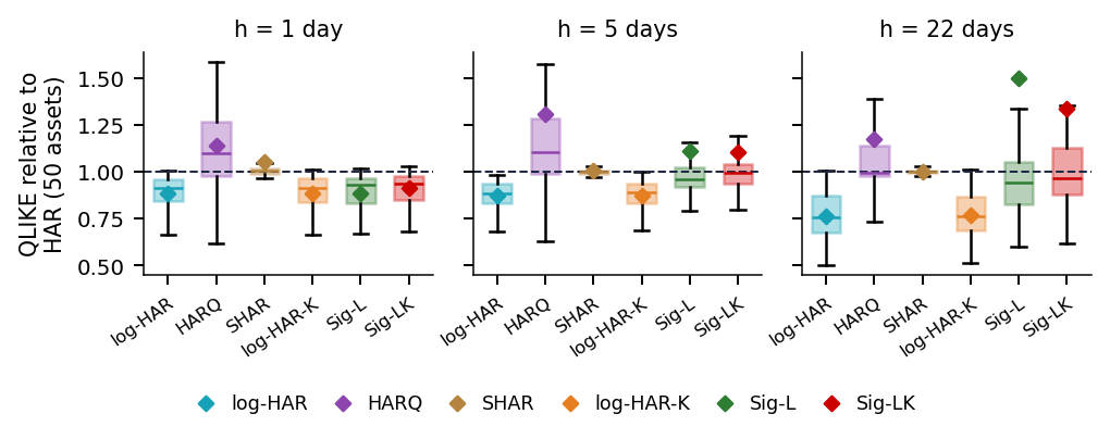

 MFM_ch20_case_study

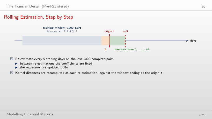
 Statistics of Financial Markets