Bucharest University of Economic Studies IDA Institute Digital Assets Blockchain Research Center AI4EFin Artificial Intelligence for Energy Finance Romanian Academy, Institute for Economic Forecasting MSCA Digital Finance
“The process of selecting a portfolio may be divided into two stages. The first stage starts with observation and experience and ends with beliefs about the future performances of available securities.” — Markowitz (1952)
16 assets and 60 months of data: 152 parameters to estimate, 16 means and 136 variances and covariances
2 000 simulated tangency portfolios: the estimated Sharpe ratio has median \(1.56\)
the true Sharpe ratio, computed with the population parameters, has median \(0.30\)
96% of them have a true Sharpe ratio below that of equal weights, 1/N (\(0.54\))
Out-of-sample, on 16 ETFs, before costs: Sharpe \(0.76\) for 1/N, between \(0.20\) and \(0.36\) for the GMV rules
The process of selecting a portfolio may be divided into two stages. The first stage starts with observation and experience and ends with beliefs about the future performances of available securities.
The paper by Markowitz (1952) deals only with the second stage: choosing the portfolio given beliefs about the securities. When the means and covariances of returns are known, it has closed-form solutions, for example the global minimum-variance (GMV) portfolio and the tangency portfolio. In applications, the first stage means estimating these parameters from data. With 16 assets, 152 parameters must be estimated, 16 means and 136 variances and covariances, from a window of 60 monthly observations. The optimiser puts large weights precisely on the assets whose parameters carry the largest estimation errors.
The chapter's simulation measures the effect of these errors. The true parameters are the moments of the nine US (United States) sectors, and each simulated sample has 60 months. Across 2,000 estimated tangency portfolios, the median absolute value of the in-sample estimated Sharpe ratio, \(|\hat\theta|\), is 1.56, while the median true Sharpe ratio, computed with the population parameters, is 0.30. Of these portfolios, 96% have a true Sharpe ratio below that of equal weights, 1/N, which is 0.54. In the same simulation, the estimated mean–variance (MV) portfolio beats 1/N only with windows of 480 months.
The out-of-sample backtest on real data points the same way. The wealth of the unconstrained MV portfolio reaches zero in all three US universes. In the combined universe of 16 ETFs, before costs, 1/N has a Sharpe ratio of 0.76 and the GMV rules between 0.20 and 0.36. The MV-LO (Mean–Variance tangency portfolio, Long-Only) rule, the long-only tangency portfolio, has the best point estimate, 0.81, but no longer beats 1/N at costs above about 22 basis points (bp). The chapter therefore studies the repairs of the inputs and the risk-based rules, which reduce the effect of estimation error, and the tests that decide whether a difference from 1/N remains significant after correcting for multiple testing.
Estimation error in 25 simulated 60-month samples from the nine US sectors: the estimated frontiers (red) lie above the true frontier (blue), while the same portfolios evaluated with the true parameters (green) lie below it; annualised volatility is on the horizontal axis and the annualised mean excess return on the vertical axis. Interactive chart: “Error Maximisation: Estimated versus Realised Frontiers (1/2)” →
What you will be able to do
Derive the GMV and tangency portfolios and the in-sample Sharpe bias.
Compute equal risk contribution (ERC) weights and net-of-cost Sharpe ratios.
Interpret why estimation error favours the 1/N rule.
Interpret a Sharpe ratio test after the correction for multiple testing.
The chapter deals with choosing the weights of a portfolio of risky assets. Classical theory gives the optimal portfolio in closed form, as a function of the means and covariances of the returns. In practice these parameters are not known but estimated from data, and the estimation errors pass into the weights. The benchmark used throughout the chapter is the equal-weight rule, 1/N, which estimates nothing. The question is whether any estimated rule beats it out of sample, after trading costs.
The theoretical results start in the next section.
Why Does Estimating the Optimum Change the Problem?
A portfolio of \(N\) assets is a weight vector \(\mathbf{w} = (w_1, \dots, w_N)^\top\) with \(\mathbf{w}^\top\mathbf{1} = 1\), where \(\mathbf{1}\) is the vector of ones. When the means and covariances of the returns are known, the optimal portfolio has a closed form. The difficulty arises when they are replaced by estimates: the optimiser puts large weights precisely on the assets whose means and covariances carry the largest estimation errors.
The size of the problem shows why the errors are large. For 16 assets, 16 means and 136 distinct variances and covariances must be estimated, 152 parameters in all. With a window of 60 monthly observations, the parameters outnumber the observations by more than two to one. The question of the chapter is whether a rule estimated under these conditions can beat equal weights out of sample, after costs.
In brief
Easy optimum, hard estimate
A portfolio is a weight vector \(\mathbf{w} = (w_1,\dots,w_N)^\top\) with \(\mathbf{w}^\top\mathbf{1} = 1\)
The optimum is easy to write with known means and covariances, hard to estimate
the optimiser loads on the largest estimation errors
16 assets: \(16\) means \(+\ 136\) variances and covariances \(= 152\) parameters, estimated from 60 monthly observations
Can any estimated rule beat equal weights out of sample, after costs?
Mean–variance optimisation with known parameters: the global minimum-variance (GMV) portfolio, the tangency portfolio, the frontier and constraints on the weights.
Measuring estimation risk and showing why Sharpe ratios computed in sample are too optimistic.
Three repairs of the inputs: covariance shrinkage, constraints and the Black–Litterman model.
Rules that use only the covariance matrix \(\boldsymbol\Sigma\): equal risk contribution (ERC) and Hierarchical Risk Parity (HRP).
Out-of-sample evaluation of the rules, with turnover, trading costs, tests of differences between Sharpe ratios and the Holm and Benjamini–Hochberg corrections for multiple testing.
Applying the methods to stocks on the Bucharest Stock Exchange (BVB).
The core path is followed by two case studies, on trading costs and on volatility timing, and by a section on research assisted by artificial intelligence (AI) and on data snooping. Detailed examples are in Further Topics, and the derivations and complete tables in the Appendix. The reference textbook is Franke, Härdle & Hafner (2019), Part I.
In brief
Core path
Mean–variance: global minimum-variance (GMV) and tangency weights, the frontier, constraints
Estimation risk: why in-sample Sharpe ratios are too optimistic
Three repairs of the inputs: covariance shrinkage, constraints, Black–Litterman
Rules that need only \(\boldsymbol\Sigma\): equal risk contribution (ERC) and Hierarchical Risk Parity (HRP)
Out-of-sample evaluation: turnover and costs, Sharpe-difference tests, Holm and Benjamini–Hochberg
The application on the Bucharest Stock Exchange (BVB)
Detailed examples and advanced topics are in Further Topics, after the Conclusions
the footer button leads there; the Back button returns to the starting slide
Deeper study
Case studies: trading costs, volatility timing
Research assisted by artificial intelligence (AI) and data snooping (searching the same data repeatedly)
The sector universe holds 9 US sector ETFs, with returns from January 1999 to July 2026. An ETF (exchange-traded fund) is a fund traded on an exchange that tracks an index.
The multi-asset universe holds 8 ETFs, with returns from May 2007 to July 2026: three equity funds, two Treasury funds, two credit funds and one gold fund.
The combined universe joins the 9 sectors and the 7 multi-asset ETFs other than SPY, which tracks the S&P 500 (Standard & Poor's), 16 ETFs in all.
The BVB universe holds 8 BVB blue chips, in lei, from October 2014 to August 2026, together with the BET (Bucharest Exchange Trading, index) and BET-TR indices.
The three US universes differ in their correlation structure. Sectors are similar assets with high correlations. The multi-asset universe holds classes with correlations of opposite sign, such as equities and Treasuries. The combined universe raises \(N\) to 16 and so amplifies estimation error. The samples start with the launch of the sector ETFs, in December 1998, and of HYG, in April 2007.
Returns are simple monthly returns computed from month-end prices, with dividends reinvested. BET (Bucharest Exchange Trading), the benchmark index of the BVB, is a price index, whereas BET-TR (total return) reinvests dividends. For the US universes, excess returns are measured over the one-month US Treasury bill (T-bill), and the benchmark is the 1/N rule. It assigns equal weights, \(w_i = 1/N\), rebalanced every month with no estimation at all. The BVB application uses BET-TR as the benchmark and assumes \(R_f = 0\).
Let \(P_{i,t}\) be the price of asset \(i\) at the end of month \(t\), adjusted for dividends and other distributions; BET remains a price index. The simple (total) return is \(R_{i,t} = P_{i,t}/P_{i,t-1} - 1\), and the excess return is \(R^e_{i,t} = R_{i,t} - R_{f,t}\), where \(R_{f,t}\) is the risk-free rate. In the seminar the same quantities are written \(r_t\) and \(r^e_t\). The log return \(\ln(P_{i,t}/P_{i,t-1}) = \ln(1 + R_{i,t})\) adds up over time but not across assets. Portfolios therefore use simple returns: the portfolio return is exactly \(R_{p,t} = \sum_i w_i R_{i,t}\).
For a portfolio of \(N\) assets, \(\mathbf{w}\) is the vector of weights, \(\boldsymbol\mu\) the vector of expected (excess) returns, \(\mathbf{1}\) the vector of ones and \(\boldsymbol\Sigma\) the \(N\times N\) covariance matrix of the returns. The portfolio mean is \(\mathbf{w}^\top\boldsymbol\mu\) and the portfolio variance is \(\mathbf{w}^\top\boldsymbol\Sigma\mathbf{w}\).
In brief
Returns
simple return \(R_{i,t} = P_{i,t}/P_{i,t-1} - 1\); \(P_{i,t}\): the month-end price of asset \(i\)
excess return \(R^e_{i,t} = R_{i,t} - R_{f,t}\) (in the seminar: \(r_t\) and \(r^e_t\)); \(R_{f,t}\): the risk-free rate
log return \(\ln(P_{i,t}/P_{i,t-1}) = \ln(1 + R_{i,t})\): adds up over time, not across assets
portfolios use simple returns, because \(R_{p,t} = \sum_i w_i R_{i,t}\) holds exactly
Portfolio of \(N\) assets
\(\mathbf{w}\): vector of weights; \(\boldsymbol\mu\): vector of expected (excess) returns; \(\mathbf{1}\): vector of ones
\(\boldsymbol\Sigma\): the \(N\times N\) covariance matrix of the returns
portfolio mean \(\mathbf{w}^\top\boldsymbol\mu\), portfolio variance \(\mathbf{w}^\top\boldsymbol\Sigma\mathbf{w}\)
The Sharpe ratio of portfolio \(p\) (Sharpe, 1966) is \(SR_p = \mathbb{E}[R^e_p]/\sigma(R^e_p)\), the mean excess return per unit of volatility \(\sigma\). Monthly figures are annualised by multiplying the mean by 12, and the volatility and the Sharpe ratio by \(\sqrt{12}\). Let \(W_t\) be wealth at time \(t\). The maximum drawdown, \(\min_t (W_t/\max_{s\le t}W_s - 1)\), is the largest relative fall of wealth from a previous peak.
An evaluation is out of sample (OOS) when the weights held in month \(t\) use only data up to month \(t-1\); it is in sample when the same data serve for estimation and for evaluation. The rules compared in the chapter are:
MV (mean–variance), the tangency portfolio computed from sample moments;
GMV, the global minimum-variance portfolio;
MV-LO and GMV-LO, their long-only (LO) versions, without short sales;
GMV-LW, the GMV portfolio computed with the Ledoit–Wolf (LW) shrunk covariance matrix;
ERC and HRP, two risk-based rules;
1/N.
In brief
Sharpe ratio (Sharpe (1966)): \(SR_p = \mathbb{E}[R^e_p]/\sigma(R^e_p)\)
the mean excess return per unit of volatility \(\sigma\)
monthly figures annualised with \(\times 12\) (mean) and \(\times\sqrt{12}\) (volatility, Sharpe)
Maximum drawdown: \(\min_t (W_t/\max_{s\le t}W_s - 1)\)
the largest fall of wealth \(W_t\) from a previous peak
Out of sample (OOS): the weights held in month \(t\) use only data up to month \(t-1\)
In sample: the same data serve for estimation and for evaluation
Rules of this chapter
MV (mean–variance): tangency portfolio from sample moments; GMV: global minimum variance
MV-LO (Mean–Variance tangency portfolio, Long-Only) and GMV-LO (Global Minimum-Variance portfolio, Long-Only): their long-only (LO) versions, with no short sales (\(w_i \ge 0\)); GMV-LW (Global Minimum-Variance portfolio with Ledoit–Wolf covariance): GMV with Ledoit–Wolf (LW) covariance shrinkage
The data cover three US universes with different correlation structures and one Romanian universe. Every rule is compared with 1/N, and the main comparison is out of sample. The next section derives the rules with known parameters, and the section on estimation risk shows what is lost when the parameters are estimated.
Mean–Variance Optimisation
This section solves the portfolio choice problem under the assumption that the parameters are known. There are \(N\) risky assets, with vector of expected excess returns \(\boldsymbol\mu\) and covariance matrix \(\boldsymbol\Sigma\), assumed positive definite. A portfolio is a weight vector \(\mathbf{w}\) with \(\mathbf{w}^\top\mathbf{1} = 1\); its mean is \(\mathbf{w}^\top\boldsymbol\mu\) and its variance \(\mathbf{w}^\top\boldsymbol\Sigma\mathbf{w}\). The horizon is a single period, negative weights are allowed until the last part of the section, and there are no transaction costs.
The problem of choosing by mean and variance is that of Markowitz (1952). The results are closed-form formulas: the global minimum-variance (GMV) portfolio, the tangency portfolio and the minimum-variance frontier (Merton, 1972). All of them are expressed through \(\boldsymbol\Sigma^{-1}\) and three scalars, \(A\),\(B\) and \(C\). They describe the choice of an investor who knows \(\boldsymbol\mu\) and \(\boldsymbol\Sigma\). In applications these parameters are estimated, and the following sections show how far the same formulas degrade when they are fed estimates. The known-parameter version is the benchmark against which this loss is measured.
Markowitz (1952) framed portfolio choice as a trade-off between two parameters of the distribution of the portfolio return: its mean and its variance. If \(\mathbf{R}\) is the vector of returns on the \(N\) assets, the portfolio return is \(R_p = \mathbf{w}^\top\mathbf{R}\), with mean \(\mathbf{w}^\top\boldsymbol\mu\) and variance \(\mathbf{w}^\top\boldsymbol\Sigma\mathbf{w}\). Other features of the distribution, such as skewness and the tails, do not enter the criterion.
The minimum-variance frontier is obtained by fixing a target mean \(m\) and searching for the fully invested portfolio with the smallest variance:
In (4.1), the constraint \(\mathbf{w}^\top\mathbf{1} = 1\) requires the whole wealth to be invested in the \(N\) assets, and the constraint \(\mathbf{w}^\top\boldsymbol\mu = m\) fixes the mean. The objective is strictly convex, because \(\boldsymbol\Sigma\) is positive definite, and the constraints are linear. If \(\boldsymbol\mu\) is not proportional to \(\mathbf{1}\), there is therefore a single optimal portfolio for every \(m\). Its variance, denoted \(\sigma^2(m)\), traces a curve in the (volatility, mean) plane.
That \(\boldsymbol\mu\) contains excess returns does not change this problem. Because the weights sum to 1, switching to total returns adds the same constant \(R_f\) to the mean of every admissible portfolio: the frontier shifts vertically and its weights stay the same.
Not every point of the curve is a rational choice. The curve has a point of minimum variance, the GMV portfolio, with mean \(\mu_{\text{GMV}}\). For a target mean \(m < \mu_{\text{GMV}}\) there is a portfolio with the same variance and a higher mean, its mirror image about \(\mu_{\text{GMV}}\); the symmetry follows from the closed form (4.11) of the frontier, derived below. Only the upper branch, \(m \ge \mu_{\text{GMV}}\), is therefore the efficient frontier.
The second formulation starts from preferences. An investor with risk aversion \(\gamma > 0\) solves
each unit of variance costs \(\gamma/2\) units of mean. For every \(\gamma\) the solution of (4.2) lies on the efficient branch. As \(\gamma\) runs over \((0, \infty)\), the solution traces the whole branch, with the GMV as the limit for \(\gamma \to \infty\). The explicit solution, (4.13), uses the scalars \(A\),\(B\) and \(C\) and is given with the closed-form frontier.
The problem does not restrict the sign of the weights. A negative weight \(w_i < 0\) is a short sale: the investor borrows asset \(i\), sells it and uses the proceeds to buy other assets. The closed-form results of this section assume that short sales are allowed and cost nothing; the constraint \(w_i \ge 0\) appears in the last part of the section.
In brief
The question of this section: which weights do we choose if \(\boldsymbol\mu\) and \(\boldsymbol\Sigma\) are known?
Markowitz (1952): investors care about the mean and the variance of portfolio returns
Minimum-variance frontier: minimum variance for every target mean \(m\)
its upper branch, \(m \ge \mu_{\text{GMV}}\) (the mean of the GMV portfolio), is the efficient frontier
The two-asset case shows the mechanism of diversification without matrix algebra. Let \(w\) be the weight of asset 1 and \(1-w\) the weight of asset 2, with volatilities \(\sigma_1\) and \(\sigma_2\) and correlation \(\rho\). The portfolio variance is
and the portfolio mean is linear in \(w\). The correlation enters only through the cross term. The lower \(\rho\), the lower the variance of every portfolio with \(0 < w < 1\).
The first-order condition \(\mathrm{d}\sigma_p^2/\mathrm{d}w = 0\) reads
The denominator of (4.4) is the variance of the difference \(R_1 - R_2\), positive outside the degenerate case \(\rho = 1\),\(\sigma_1 = \sigma_2\), so \(w^*\) is a minimum. The numerator shows that \(w^*\) is negative when \(\rho > \sigma_2/\sigma_1\). If the more volatile asset is sufficiently correlated with the other one, minimum variance requires selling it short.
Two limiting cases of (4.3) fix the intuition. For \(\rho = 1\),\(\sigma_p = |w\sigma_1 + (1-w)\sigma_2|\): when \(0 \le w \le 1\), the portfolio volatility is the weighted average of the volatilities and diversification does not reduce risk. For \(\rho = -1\),\(\sigma_p = |w\sigma_1 - (1-w)\sigma_2|\), which vanishes at \(w = \sigma_2/(\sigma_1 + \sigma_2)\): two perfectly negatively correlated risky assets form a riskless portfolio.
The interactive chart has the annualised volatility on the horizontal axis and the annualised mean of total returns on the vertical axis. The two assets are SPY (US equities) and TLT (long-term US Treasuries), with parameters estimated on monthly data over 2002–2026. Each curve contains the portfolios with \(0 \le w \le 1\) for a given correlation. The dashed curve corresponds to a correlation of 1, and the solid curve to the correlation chosen with the first slider. The diamond marks the minimum-variance portfolio with an SPY weight between 0 and 1, and the red dot the portfolio with the SPY weight chosen with the second slider. The ▶ button lowers the correlation from 1 to −1.
Question for the room The annual volatilities are 14.7% for SPY and 13.5% for TLT. The ▶ button lowers their correlation from 1 to −1. How does the volatility of the minimum-variance portfolio change?
Answer
It falls from 13.5% to zero. At a correlation of 1, the minimum-variance portfolio is TLT alone; below a correlation of 0.92 (the ratio 13.5/14.7) it also holds SPY. At the estimated correlation, −0.10, it holds 46% in SPY and has a volatility of 9.4%. At −1, with 48% in SPY, the volatility is zero. Portfolio volatility equals the weighted average of the volatilities only when the correlation is 1.
In the data, the annual volatilities are 14.7% for SPY and 13.5% for TLT, and the estimated correlation is \(\rho = -0.10\). Formula (4.4) gives \(w^* = 46\%\) in SPY and a volatility of 9.4%, lower than the volatility of either asset.
As the correlation falls from 1 to −1, the volatility of the minimum-variance portfolio falls from 13.5% to zero. At high correlations, the minimum with weights between 0 and 1 is TLT alone, because \(w^*\) would be negative. SPY enters the portfolio below the threshold \(\rho = \sigma_{\text{TLT}}/\sigma_{\text{SPY}} = 13.5/14.7 \approx 0.92\). At \(\rho = -1\), the SPY weight is 48% and the volatility is zero.
The correlation between equities and government bonds varies over time, and its models are the subject of Chapter 6. With \(N\) assets the same mechanism works through all the covariances, and the next part writes the problem in matrix form.
The global minimum-variance (GMV) portfolio is the leftmost point of the frontier. Among all fully invested portfolios it has the smallest variance, whatever its mean. The problem drops the constraint on the mean and keeps only the budget:
Let \(\lambda\) be the Lagrange multiplier of the budget constraint in (4.5). The Lagrangian is \(\mathcal{L}(\mathbf{w}, \lambda) = \mathbf{w}^\top\boldsymbol\Sigma\mathbf{w} - \lambda(\mathbf{w}^\top\mathbf{1} - 1)\), and its gradient with respect to \(\mathbf{w}\) is \(2\boldsymbol\Sigma\mathbf{w} - \lambda\mathbf{1}\). Setting the gradient to zero gives \(\mathbf{w} = \tfrac{\lambda}{2}\boldsymbol\Sigma^{-1}\mathbf{1}\); the inverse exists because \(\boldsymbol\Sigma\) is positive definite. Premultiplying by \(\mathbf{1}^\top\) and using the budget gives
The objective is convex and the constraint is linear, so the first-order condition is also sufficient: the point found is the unique minimum. The same point is the vertex of the closed-form frontier of Merton (1972),(4.11) below.
By (4.6), the weight of asset \(i\) is proportional to the sum of the entries in row \(i\) of \(\boldsymbol\Sigma^{-1}\). Nothing in the formula fixes the sign of this sum, so the GMV can contain short positions, as in the two-asset example for \(\rho > \sigma_2/\sigma_1\). The mean of the portfolio is \(\mu_{\text{GMV}} = \mathbf{w}_{\text{GMV}}^\top\boldsymbol\mu = B/A\), with \(B = \mathbf{1}^\top\boldsymbol\Sigma^{-1}\boldsymbol\mu\); the scalar \(B\) reappears with the tangency portfolio.
The solution (4.6) does not contain \(\boldsymbol\mu\). Means are estimated far less precisely than covariances (Merton, 1980); the argument is given in the next section. This is why the GMV reappears in the chapter as GMV-LO (long-only) and as GMV-LW, with the covariance shrinkage of Ledoit & Wolf (2004b).
The tangency portfolio is the fully invested portfolio with the highest Sharpe ratio (Sharpe, 1966). Here \(\boldsymbol\mu\) must be the vector of expected returns in excess of the riskless rate, because the Sharpe ratio measures the mean excess return per unit of volatility. The problem is
The function \(S\) does not depend on the scale of \(\mathbf{w}\), only on its direction and sign: for every \(c \neq 0\),\(S(c\,\mathbf{w}) = \operatorname{sign}(c)\,S(\mathbf{w})\). The budget constraint in (4.7) therefore fixes only the scale, and the problem reduces to the choice of a direction. The gradient of \(S\) is
and setting it to zero gives the condition \(\boldsymbol\mu = \frac{\mathbf{w}^\top\boldsymbol\mu}{\mathbf{w}^\top\boldsymbol\Sigma\mathbf{w}}\,\boldsymbol\Sigma\mathbf{w}\). The factor in front of \(\boldsymbol\Sigma\mathbf{w}\) is a scalar, so \(\mathbf{w} \propto \boldsymbol\Sigma^{-1}\boldsymbol\mu\). Dividing by the sum of the components gives
\[\mathbf{w}_{\text{MV}} = \frac{\boldsymbol\Sigma^{-1}\boldsymbol\mu}{B}, \qquad B = \mathbf{1}^\top\boldsymbol\Sigma^{-1}\boldsymbol\mu.\]
(4.8)
The maximum value follows from the Cauchy–Schwarz inequality. Let \(\boldsymbol\Sigma^{1/2}\) be the symmetric square root of \(\boldsymbol\Sigma\). From \(\mathbf{w}^\top\boldsymbol\mu = (\boldsymbol\Sigma^{1/2}\mathbf{w})^\top(\boldsymbol\Sigma^{-1/2}\boldsymbol\mu)\),
so \(|S(\mathbf{w})| \le \theta\), with \(\theta^2 = \boldsymbol\mu^\top\boldsymbol\Sigma^{-1}\boldsymbol\mu\). Equality holds only for \(\mathbf{w}\) proportional to \(\boldsymbol\Sigma^{-1}\boldsymbol\mu\): the direction \(\boldsymbol\Sigma^{-1}\boldsymbol\mu\) attains \(+\theta\) and the opposite direction attains \(-\theta\). Unlike the GMV, the result depends on both \(\boldsymbol\mu\) and \(\boldsymbol\Sigma\).
Normalising to the budget in (4.8) can reverse the direction. The mean of \(\mathbf{w}_{\text{MV}}\) is \(\theta^2/B\) and its volatility is \(\theta/|B|\), so its Sharpe ratio is \(\operatorname{sign}(B)\,\theta\). If \(B > 0\),\(\mathbf{w}_{\text{MV}}\) is the maximum-Sharpe portfolio. If \(B < 0\), dividing by \(B\) flips the sign, and \(\mathbf{w}_{\text{MV}}\) is the fully invested portfolio with the lowest Sharpe ratio, \(-\theta\). If \(B = 0\), the optimal direction has weights summing to zero and cannot be scaled so that the weights sum to 1.
The sign of \(B\) has a direct interpretation. From the previous part, \(B = A\,\mu_{\text{GMV}}\) with \(A > 0\), so \(B > 0\) exactly when the GMV portfolio has a positive expected excess return. A calculation that applies \(\boldsymbol\Sigma^{-1}\boldsymbol\mu/B\) without checking the sign of \(B\) can return the minimum-Sharpe portfolio. With estimated parameters, the denominator \(\mathbf{1}^\top\hat{\boldsymbol\Sigma}^{-1}\hat{\boldsymbol\mu}\) can be close to zero, and the estimated tangency weights then have very heavy tails (appendix on the distribution of the weights).
In brief
The problem: \(\max_{\mathbf{w}} \mathbf{w}^\top\boldsymbol\mu/\sqrt{\mathbf{w}^\top\boldsymbol\Sigma\mathbf{w}}\) s.t. \(\mathbf{w}^\top\mathbf{1} = 1\)
\(\boldsymbol\mu\): the expected excess returns
First-order condition: \(\boldsymbol\mu = \dfrac{\mathbf{w}^\top\boldsymbol\mu}{\mathbf{w}^\top\boldsymbol\Sigma\mathbf{w}}\,\boldsymbol\Sigma\mathbf{w}\), so \(\mathbf{w} \propto \boldsymbol\Sigma^{-1}\boldsymbol\mu\)
The budget gives \(\mathbf{w}_{\text{MV}} = \boldsymbol\Sigma^{-1}\boldsymbol\mu/B\), with \(B = \mathbf{1}^\top\boldsymbol\Sigma^{-1}\boldsymbol\mu\)
Maximum Sharpe ratio \(\theta\): \(\theta^2 = \boldsymbol\mu^\top\boldsymbol\Sigma^{-1}\boldsymbol\mu\)
needs \(\boldsymbol\mu\) and \(\boldsymbol\Sigma\)
The Sharpe ratio of \(\mathbf{w}_{\text{MV}}\) is \(\operatorname{sign}(B)\,\theta\): the maximum only if \(B > 0\)
Tobin (1958) adds a riskless asset paying \(R_f\). In the (volatility, excess mean) plane this asset sits at the origin. A portfolio that invests the fraction \(\alpha \ge 0\) in the risky portfolio \(\mathbf{w}\) and the rest in the riskless asset has excess mean \(\alpha\,\mathbf{w}^\top\boldsymbol\mu\) and volatility \(\alpha\sqrt{\mathbf{w}^\top\boldsymbol\Sigma\mathbf{w}}\). The mixes therefore lie on a ray from the origin whose slope is the Sharpe ratio of \(\mathbf{w}\). The steepest ray passes through the tangency portfolio and has slope \(\theta\) from (4.9);\(\alpha > 1\) means borrowing at the rate \(R_f\).
We now assume \(B > 0\), so the fully invested tangency portfolio has Sharpe ratio \(+\theta\). Let \(m_T\) and \(\sigma_T\) be its excess mean and volatility. An investor with risk aversion \(\gamma\) chooses \(\alpha\) to maximise \(\alpha m_T - \frac{\gamma}{2}\alpha^2\sigma_T^2\), which gives
\[\alpha^* = \frac{m_T}{\gamma\,\sigma_T^2}.\]
(4.10)
Because \(m_T > 0\), the solution (4.10) satisfies \(\alpha \ge 0\); for an arbitrary risky fund subject to this constraint, the solution is \(\alpha^* = \max\{0,\ m_T/(\gamma\sigma_T^2)\}\). By (4.10), risk aversion changes only the share invested in the risky part, not its composition: this is two-fund separation. If all investors use the same \(\boldsymbol\mu\) and \(\boldsymbol\Sigma\), they all hold the same risky portfolio. This is the bridge to the Capital Asset Pricing Model (CAPM), covered in Chapter 3.
Without a riskless asset, the frontier has a closed form (Merton, 1972). The problem with two constraints has the Lagrangian
and the first-order condition gives \(\mathbf{w} = \lambda_1\boldsymbol\Sigma^{-1}\boldsymbol\mu + \lambda_2\boldsymbol\Sigma^{-1}\mathbf{1}\). With \(A\) and \(B\) from the previous parts and \(C = \boldsymbol\mu^\top\boldsymbol\Sigma^{-1}\boldsymbol\mu = \theta^2\), the two constraints become a \(2\times 2\) linear system:
\[\lambda_1 C + \lambda_2 B = m, \qquad \lambda_1 B + \lambda_2 A = 1.\]
Its solution is \(\lambda_1 = (Am - B)/D\) and \(\lambda_2 = (C - Bm)/D\), with \(D = AC - B^2\). The minimum variance follows from \(\mathbf{w}^\top\boldsymbol\Sigma\mathbf{w} = \mathbf{w}^\top(\lambda_1\boldsymbol\mu + \lambda_2\mathbf{1}) = \lambda_1 m + \lambda_2\):
The condition \(D > 0\) is another Cauchy–Schwarz inequality, this time for the inner product defined by \(\boldsymbol\Sigma^{-1}\):\(B^2 = (\mathbf{1}^\top\boldsymbol\Sigma^{-1}\boldsymbol\mu)^2 \le (\mathbf{1}^\top\boldsymbol\Sigma^{-1}\mathbf{1})(\boldsymbol\mu^\top\boldsymbol\Sigma^{-1}\boldsymbol\mu) = AC\). Equality holds only if \(\boldsymbol\mu\) is proportional to \(\mathbf{1}\). In that case all fully invested portfolios have the same mean, and the frontier collapses to the GMV portfolio.
The second form in (4.11) shows the geometry. In the \((\sigma^2, m)\) plane, \(\sigma^2(m)\) is a parabola with vertex at \((1/A,\ B/A)\), that is, at the GMV portfolio. In the \((\sigma, m)\) plane of the charts, the same relation is a hyperbola. The curve is symmetric about \(m = B/A\), which justifies taking the upper branch as the efficient frontier.
The frontier weights combine two portfolios already computed. Since \(\boldsymbol\Sigma^{-1}\mathbf{1} = A\,\mathbf{w}_{\text{GMV}}\) and \(\boldsymbol\Sigma^{-1}\boldsymbol\mu = B\,\mathbf{w}_{\text{MV}}\), for \(B \neq 0\)
\[\mathbf{w}(m) = \lambda_1 B\,\mathbf{w}_{\text{MV}} + \lambda_2 A\,\mathbf{w}_{\text{GMV}}, \qquad \lambda_1 B + \lambda_2 A = 1.\]
(4.12)
The coefficients in (4.12) sum to 1, but one of them can be negative. More generally, any two distinct frontier portfolios generate the whole frontier (Merton, 1972).
The same algebra completes the utility formulation (4.2) from the first part of the section. Its first-order condition gives
The portfolio \(\mathbf{w}_\gamma\) in (4.13) has the form \(\lambda_1\boldsymbol\Sigma^{-1}\boldsymbol\mu + \lambda_2\boldsymbol\Sigma^{-1}\mathbf{1}\), so it lies on the frontier. Its mean falls from \(+\infty\) towards \(B/A\) as \(\gamma\) rises from 0 towards \(\infty\), so the solutions trace the efficient branch.
The formulas are now applied to the nine US sector ETFs, with monthly excess returns from January 1999 to July 2026 (\(T = 331\) months). The parameters \(\boldsymbol\mu\) and \(\boldsymbol\Sigma\) are replaced by the sample mean and the sample covariance matrix, computed on the full sample. The picture is therefore in-sample: the weights are chosen with the same data on which they are evaluated, as if the investor had known in 1999 the means and covariances realised up to 2026.
Monthly means are annualised with the factor 12, and volatilities and Sharpe ratios with the factor \(\sqrt{12}\); the axes are in decimals. On the interactive chart, the curve "Frontier, short sales allowed" is the unconstrained frontier, and the curve "Frontier, long-only" is the frontier with \(w_i \ge 0\). The circles mark the individual sectors, and the two stars mark the tangency portfolios, with and without short sales. The slope of the line joining the origin to a star is the Sharpe ratio of that portfolio. The bar chart below gives the weights of the two tangency portfolios.
The slider chooses how many sectors enter the optimisation, and ▶ adds them one by one; the curve "Frontier, all 9 sectors" stays as a reference. The long-only frontier lies to the right of the unconstrained frontier or touches it, because the set of admissible portfolios is smaller.
Question for the room With short selling allowed, does the tangency portfolio hold a long position in every sector with a positive mean return?
Answer
No. The tangency portfolio is short XLF (−37%) and XLB (−21%), although both have positive means. The sign of a weight depends on the whole vector of means and on the covariances: the 0.85 correlation of XLB with XLI (Industrial Select Sector SPDR Fund) or the low Sharpe ratio of XLF do not explain it on their own. The long-only constraint lowers the Sharpe ratio from 0.66 to 0.61.
The annualised Sharpe ratio is 0.66 for the tangency portfolio, 0.57 for the GMV, whose volatility is 11.1%, and 0.54 for 1/N. The tangency portfolio reaches this maximum through short positions in financials (\(-0.37\)) and materials (\(-0.21\)), although both sectors have positive means. The largest long position is in health care (\(+0.37\)).
By (4.8), the sign of a weight depends on the whole vector \(\boldsymbol\Sigma^{-1}\boldsymbol\mu\), not only on the sector's own mean. Neither the 0.85 correlation between materials and industrials nor the low Sharpe ratio of financials explains the short positions on its own.
With the long-only constraint, the Sharpe ratio of the tangency portfolio falls to 0.61. Materials, financials and industrials receive exactly zero weight: the constraint \(w_i \ge 0\) is active for them, and the optimum lies on the boundary of the admissible set, in a corner solution.
The difference between 0.66 and 0.54 is the gain of the best fixed combination of the sectors, chosen with the whole history known in advance. A rule that estimates the parameters from the past alone does not have this information. The next section measures how much such a rule loses.
In brief
Monthly excess returns, January 1999 – July 2026 (\(T = 331\))
axes annualised, in decimals
all parameters estimated on the full sample: an in-sample picture
The formulas so far allow any weight. The basic constraint is long-only (LO): \(w_i \ge 0\) for every asset. Other linear constraints limit concentration: position caps, for example \(w_i \le 0.2\), and group caps, \(\sum_{i\in G} w_i \le c_G\), where \(G\) is a group of assets (a sector or an asset class) and \(c_G\) its cap.
A leverage limit concerns the gross exposure \(\sum_i |w_i|\). Because the weights sum to 1,
\[\sum_i |w_i| = 1 + 2\sum_i \max(-w_i, 0),\]
(4.14)
so the gross exposure exceeds 1 by twice the sum of the short positions. By (4.14), the constraint \(\sum_i |w_i| \le L\) with \(L = 1\) is therefore equivalent to ruling out short sales.
With inequalities the closed forms no longer hold. The optimality conditions add a multiplier \(\lambda_i \ge 0\) for each constraint \(w_i \ge 0\), equal to zero when the constraint is not active (\(w_i > 0\)). Which constraints are active is not known in advance; it follows from the solution. For the GMV, the long-only problem (GMV-LO) is
The objective remains quadratic and convex, and the constraints are linear, as for the long-only frontier. The problem is one of quadratic programming, solved numerically.
Constraints cannot improve the in-sample optimum: on the US sectors, the Sharpe ratio of the tangency portfolio falls from 0.66 to 0.61. Out of sample the effect can go the other way. Frost & Savarino (1988) showed that constraining the weights improved out-of-sample performance. Jagannathan & Ma (2003) explained the mechanism: the solution of (4.15) is the GMV portfolio (4.6) of a modified covariance matrix. An active constraint \(w_i \ge 0\) is equivalent to shrinking the estimated covariances of asset \(i\), that is, to shrinkage of the covariance matrix. The proof and a two-asset example are in the shrinkage section (Constraints Are Shrinkage Too).
In brief
Long-only (LO): \(w_i \ge 0\)
no closed form, solved by quadratic programming
Position limits: \(w_i \le 0.2\)
sector or asset-class limits: \(\sum_{i\in G} w_i \le c_G\)
With known parameters, mean–variance allocation has explicit solutions. The GMV portfolio (4.6) uses only the covariances. The tangency portfolio (4.8) has the maximum Sharpe ratio \(\theta = \sqrt{\boldsymbol\mu^\top\boldsymbol\Sigma^{-1}\boldsymbol\mu}\) only if \(B > 0\). The frontier (4.11) is a hyperbola determined by \(A\),\(B\) and \(C\), and any two of its distinct portfolios generate it (Merton, 1972). With a riskless asset, all investors combine the same tangency portfolio with the riskless asset (Tobin, 1958). Constraints on the weights remove the closed forms and require quadratic programming.
On the US sectors, even with parameters estimated on the full sample, the tangency portfolio raises the Sharpe ratio only from 0.54 (1/N) to 0.66. All the formulas of this section assume that \(\boldsymbol\mu\) and \(\boldsymbol\Sigma\) are known. The next section replaces them with estimates and shows how estimation errors pass into the weights and the Sharpe ratio.
Estimation Risk
The previous section assumed that \(\boldsymbol\mu\) and \(\boldsymbol\Sigma\) are known. Here they are replaced by sample (plug-in) estimates, and the question is how much the optimal portfolio loses through this substitution. The answer has four parts:
Means are estimated far less precisely than variances, whatever the sampling frequency.
Simulation shows that estimated frontiers are systematically too optimistic and that the portfolios chosen on them have poor true performance.
Quantifying the bias of the estimated maximum Sharpe ratio.
The instability of the weights on real data and the length of the estimation window that the mean–variance rule would need to beat 1/N.
Throughout the section, a simulation means the following experiment:
The "true" parameters are the moments of the US sectors over 1999–2026;
Samples of returns are drawn from the Normal distribution with these parameters;
The weights are computed from the moments of each sample;
The weights are evaluated with the true parameters.
The gap between the estimated and the true Sharpe ratio of the same portfolio measures the effect of estimation error.
Merton (1980) compares the precision with which the mean and the variance of returns can be estimated. Consider a sample of \(Y\) years, observed \(h\) times a year, with i.i.d. returns from the Normal distribution (a diffusion), with annual mean \(\mu\) and annual variance \(\sigma^2\). Each of the \(hY\) returns has mean \(\mu/h\) and variance \(\sigma^2/h\). The natural estimator of the annual mean is the sum of all returns divided by \(Y\), and its variance is \(hY(\sigma^2/h)/Y^2\). For the variance, the sample estimator has, under the Normal distribution, approximate variance \(2\sigma^4/(hY)\):
The argument uses additive increments of a constant-parameter diffusion. The first relation in (4.16) does not depend on \(h\): in such a model, increasing the observation frequency over a fixed calendar span does not reduce the variance of the mean estimator, whose precision grows only with the span of the sample, in years. The second relation tends to zero as \(h \to \infty\): in the idealised model, the variance can be estimated as precisely as desired over a fixed interval if the observations are frequent enough. For simple returns, the realised annual return compounds as \(\prod_t(1 + R_t) - 1\); it is not the sum of the monthly returns. Without Normality, \(\operatorname{Var}(\hat\sigma^2) \approx (\kappa - 1)\sigma^4/(hY)\), where \(\kappa\) is the kurtosis of the returns; for the Normal distribution, \(\kappa = 3\). The general formula requires a finite fourth moment, an assumption questioned in Chapter 1.
For SPY, with \(Y = 24\) years and \(\sigma = 14.7\%\), the standard error of the annual mean is \(0.147/\sqrt{24}\), that is 3.0%. The 95% confidence interval for the estimated mean of 11.7% is [5.8%, 17.6%]: the data are compatible with means that differ by a factor of three. By (4.16), a standard error of 1% would require \((0.147/0.01)^2\), about 217 years of data.
Chopra & Ziemba (1993) measured the consequence for portfolio choice: in the configurations the authors analyse, errors in the means cost about ten times more than errors in the variances. It follows that rules which do not use estimated means, such as GMV and risk parity, are more robust to estimation error than the tangency portfolio.
The question of this section: how much does the optimal portfolio lose when \(\boldsymbol\mu\) and \(\boldsymbol\Sigma\) are replaced by estimates?
Merton (1980): \(Y\) years sampled \(h\) times a year
i.i.d. Normal returns (a diffusion) with annual mean \(\mu\) and variance \(\sigma^2\)
\(\operatorname{Var}(\hat\mu) = \sigma^2/Y\): independent of \(h\); only the span of the sample helps
\(\operatorname{Var}(\hat\sigma^2) \approx 2\sigma^4/(hY) \to 0\) as \(h \to \infty\) (Normal; in general \((\kappa - 1)\sigma^4/(hY)\), \(\kappa\) the kurtosis)
the general formula requires a finite fourth moment, which Chapter 1 questions
SPY, \(Y = 24\), \(\sigma = 14.7\%\): standard error \(3.0\%\)
95% interval \([5.8\%, 17.6\%]\) for a mean of \(11.7\%\)
A standard error of \(1\%\) needs \((0.1472/0.01)^2 \approx 217\) years
Chopra & Ziemba (1993): errors in means cost about ten times more than errors in variances
rules without means (GMV, risk parity) are more robust
Error Maximisation: Estimated versus Realised Frontiers (1/2)
The interactive chart runs the simulation described in the introduction to this section. The first panel has the annualised volatility on the horizontal axis and the annualised mean excess return on the vertical axis. The blue curve is the true frontier, computed with the population parameters. Each red curve is the frontier estimated from one simulated sample, and the paired green curve holds the same portfolios evaluated with the true parameters: the realised frontier.
The drop-down list sets the sample length, 60 months by default, the slider sets how many of the 25 samples are drawn, and the "New samples" button draws others. The second panel is the histogram of the true Sharpe ratio of the estimated tangency portfolio over 500 samples; the 1/N line marks the Sharpe ratio of equal weights, and the dashed "optimum" line that of the true tangency portfolio.
Question for the room With 60 months of data, how often does the estimated tangency portfolio beat 1/N?
Answer
In about 4% of the samples. In the simulation on this page, 18 of the 500 portfolios (3.6%) beat 1/N; in the lecture, with 2,000 portfolios, 4%. The median Sharpe ratio evaluated with the true parameters is 0.30, against 0.54 for 1/N. The in-sample estimated Sharpe ratio has median 1.51 on this page; in the lecture, the median of its absolute value, |θ̂|, is 1.56.
The red frontiers lie above the true frontier, and the green ones all lie below it. In the simulation on this page, 18 of the 500 estimated tangency portfolios, 3.6%, have a true Sharpe ratio above that of 1/N. The median signed in-sample Sharpe ratio is 1.51, and the median true Sharpe ratio is 0.30, against 0.54 for 1/N.
In brief
Michaud (1989): optimisers are estimation-error maximisers
Michaud (1989) called mean–variance optimisers estimation-error maximisers. The optimiser looks for the combination with the highest estimated Sharpe ratio. Assets whose means are overestimated or whose covariances are underestimated look more attractive than they are, and the optimiser selects precisely those. The estimated frontier therefore reflects, besides the true parameters, the most favourable estimation errors of the sample. Best & Grauer (1991) showed the same sensitivity from the other side: a small change in a single estimated mean moves many weights of the optimal portfolio.
The lecture's simulation uses 2000 tangency portfolios estimated from samples of 60 months. The median of \(\hat\theta\), the absolute value of the in-sample Sharpe ratio, is 1.56 a year. Evaluated with the true parameters, the same portfolios have a median signed Sharpe ratio of 0.30, although the true optimum is 0.66. Of these portfolios, 96% have a true Sharpe ratio below that of 1/N, 0.54, and 7.5% have a negative true Sharpe ratio.
Part of these results comes from the sign problem discussed with the tangency portfolio. In 11% of the samples, \(\hat B = \mathbf{1}^\top\hat{\boldsymbol\Sigma}^{-1}\hat{\boldsymbol\mu} < 0\), where \(\hat{\boldsymbol\mu}\) and \(\hat{\boldsymbol\Sigma}\) are the sample estimates. In these samples, the tangency formula (4.8) applied to the estimates returns the portfolio with the minimum estimated Sharpe ratio. The signed in-sample Sharpe ratio of the budget-normalised portfolio is therefore \(\operatorname{sign}(\hat B)\,\hat\theta\), and when \(\hat B < 0\),\(\hat\theta\) is not the Sharpe ratio of the fully invested portfolio chosen.
In brief
2000 simulated tangency portfolios: median estimated maximum Sharpe \(1.56\)
median true Sharpe \(0.30\), true optimum \(0.66\)
\(96\%\) have a true Sharpe below 1/N (\(0.54\)), \(7.5\%\) below zero
In \(11\%\) of samples \(\hat B = \mathbf{1}^\top\hat{\boldsymbol\Sigma}^{-1}\hat{\boldsymbol\mu} < 0\)
so the tangency formula returns the minimum-Sharpe portfolio
The simulation shows that the estimated maximum Sharpe ratio is far too high. Kan & Zhou (2007) give the exact expression of this bias. Excess returns are i.i.d. \(N(\boldsymbol\mu, \boldsymbol\Sigma)\), observed over \(T\) months, for \(N\) assets. Let \(\hat{\boldsymbol\mu}\) and \(\hat{\boldsymbol\Sigma}\) be the maximum-likelihood estimators, and
the in-sample squared maximum Sharpe ratio, the plug-in estimator of \(\theta^2 = \boldsymbol\mu^\top\boldsymbol\Sigma^{-1}\boldsymbol\mu\) from (4.9).
Under these assumptions, \(\hat{\boldsymbol\mu} \sim N(\boldsymbol\mu, \boldsymbol\Sigma/T)\), and \(T\hat{\boldsymbol\Sigma}\) has a Wishart distribution with \(T-1\) degrees of freedom, the matrix analogue of the \(\chi^2\) distribution; the two estimators are independent. For \(T > N + 2\), the inverse Wishart moment is \(\mathbb{E}[\hat{\boldsymbol\Sigma}^{-1}] = \frac{T}{T-N-2}\boldsymbol\Sigma^{-1}\) (appendix on Wishart moments). Conditioning on \(\hat{\boldsymbol\mu}\) and using \(\mathbb{E}[\mathbf{x}^\top\mathbf{K}\mathbf{x}] = \operatorname{tr}(\mathbf{K}\operatorname{Var}(\mathbf{x})) + \mathbb{E}[\mathbf{x}]^\top\mathbf{K}\,\mathbb{E}[\mathbf{x}]\) for the random vector \(\mathbf{x} = \hat{\boldsymbol\mu}\) and the fixed matrix \(\mathbf{K} = \boldsymbol\Sigma^{-1}\), where \(\operatorname{tr}\) is the trace, gives
\[\mathbb{E}[\hat\theta^2] = \frac{T}{T-N-2}\Big(\theta^2 + \frac{N}{T}\Big) = \frac{T\theta^2 + N}{T - N - 2}, \qquad T > N + 2.\]
(4.17)
Equations (4.17) and (4.18) use the covariance estimator with divisor \(T\). With divisor \(T-1\), used in the simulation, the expectation of \(\hat\theta^2\) becomes \(\frac{T-1}{T-N-2}\big(\theta^2 + \frac{N}{T}\big)\). Formula (4.17) contains two sources of upward bias. The term \(N/T\) comes from the noise in the estimated means: even with \(\theta = 0\), the \(N\) estimated means are not all zero, and the optimiser exploits them. The factor \(T/(T-N-2) > 1\) comes from inverting the estimated covariance matrix. Both grow with the ratio \(N/T\).
On the US sectors, with \(N = 9\),\(T = 60\) and \(\theta = 0.66\) a year in the simulation, the factor \(T/(T-N-2)\) is 1.22, and (4.17) gives \(\sqrt{12\,\mathbb{E}[\hat\theta^2]} = 1.65\) a year. This figure is a root mean square, not a median. The simulated median of the previous part, 1.56, is lower because the distribution of \(\hat\theta\) is right-skewed.
\(\hat\theta^2 = \hat{\boldsymbol\mu}^\top\hat{\boldsymbol\Sigma}^{-1}\hat{\boldsymbol\mu}\): the in-sample squared maximum Sharpe ratio, from the maximum-likelihood \(\hat{\boldsymbol\mu}\), \(\hat{\boldsymbol\Sigma}\); \(\theta^2\): its true value
\[ \mathbb{E}[\hat\theta^2] = \frac{T}{T-N-2}\Big(\theta^2 + \frac{N}{T}\Big) = \frac{T\theta^2 + N}{T - N - 2}, \qquad T > N + 2 \]
Sectors: \(N = 9\), \(T = 60\), true \(\theta = 0.66\) a year: \(\sqrt{12\,\mathbb{E}[\hat\theta^2]} = 1.65\) a year
a root mean square, not a median
the simulated median \(1.56\) is lower: \(\hat\theta\) is right-skewed; derivation: Seminar 4, A8
The estimator (4.18) can be negative, although \(\theta^2 \ge 0\);\(\sqrt{\hat\theta^2_u}\) is then not even real. Truncating it at zero gives a nonnegative but upward-biased estimator. The real-valued estimator \(\sqrt{\max(0,\ \hat\theta^2_u)}\) of \(\theta\) is nonnegative but generally biased.
On the US sectors, over the full sample (\(T = 331\)) and under i.i.d. Normality, the bias correction of \(\hat\theta^2\) lowers the equivalent point estimate of the Sharpe ratio from 0.66, the plug-in value, to about 0.31 a year. The correction concerns \(\theta^2\), not a particular portfolio: it does not show which part of the observed Sharpe ratio of the tangency portfolio is noise.
The sample tangency weights can also be obtained from a regression (Britten-Jones, 1999). Let \(\mathbf{r}_t\) be the vector of excess returns in month \(t\) and \(u_t\) the regression error. Regressing the constant 1 on the excess returns, without an intercept, by ordinary least squares (OLS) gives the coefficients \(\mathbf{b}\), and
The weights (4.19) are the sample tangency weights, because the OLS coefficients are proportional to \(\hat{\boldsymbol\Sigma}^{-1}\hat{\boldsymbol\mu}\). The advantage of this formulation is that inference on the weights becomes inference on regression coefficients: the \(t\)-test of \(b_i = 0\) checks whether asset \(i\) has a zero weight in the tangency portfolio. The derivation and the tests on the sectors are in the appendix on the Britten-Jones regression.
In brief
Unbiased estimator of \(\theta^2\): \(\hat\theta^2_u = \big[(T-N-2)\,\hat\theta^2 - N\big]/T\)
It can be negative; truncating at zero gives a nonnegative but upward-biased estimator, and \(\sqrt{\hat\theta^2_u}\) is not unbiased for \(\theta\)
Sectors, full sample (\(T = 331\)), under i.i.d. Normality: the bias correction of \(\hat\theta^2\) lowers the equivalent point estimate of the Sharpe ratio from \(0.66\) (plug-in) to about \(0.31\) a year
the correction concerns \(\theta^2\): it does not show which part of the observed Sharpe ratio is noise
The simulations so far use known parameters and Normal returns. The interactive chart shows the same phenomenon on real data. For every month, the MV and GMV-LW weights of the nine sectors are estimated on the previous 60 months, that is, on a 60-month rolling window.
The first panel shows, for the month chosen with the slider, the weights of the two rules, sector by sector; the vertical axis is in per cent. The second panel shows, for every month, the gross exposure, the sum of the absolute values of the weights, on a log scale; the dotted line marks the chosen month. The ▶ button runs through the months.
Question for the room How large do mean–variance weights become when they are re-estimated each month on the last 60 months?
Answer
In July 2026, the last month, the gross exposure (sum of absolute weights) is 7.1 for MV and 1.9 for GMV-LW: shrinkage does not eliminate short positions. Over the whole period, the medians are 4.9 for MV and 1.5 for GMV-LW. The largest absolute MV weight is 26; in 90% of the months the MV gross exposure exceeds 3.
In July 2026, the last month, the gross exposure is 7.1 for MV and 1.9 for GMV-LW. Covariance shrinkage does not eliminate the short positions of GMV-LW, but it keeps them several times smaller than those of MV.
The 60-month window is one of the two windows used by DeMiguel, Garlappi & Uppal (2009), who use 60 and 120 months. The choice of window is a trade-off: a longer window reduces estimation error, and a shorter one tracks regime changes faster. A rolling window produces exactly the small changes in the estimated means that move many weights at once: from one month to the next, one observation enters the window and one leaves it.
On the nine sectors, the median gross exposure of MV is \(\sum_i |w_i| = 4.9\), and it exceeds 3 in 90% of the months. By (4.14), a gross exposure of 4.9 means short positions that add up to almost twice the invested wealth. The largest single MV weight reaches 26 in absolute value.
The extreme jumps occur in 2004–2006 and in 2009. In those windows, the denominator \(\mathbf{1}^\top\hat{\boldsymbol\Sigma}^{-1}\hat{\boldsymbol\mu}\) of the tangency weights is close to zero, and the weights have very heavy tails. The denominator is negative in 12 of the 271 windows; in those months MV holds the portfolio with the minimum estimated Sharpe ratio.
GMV-LW, which uses no means and shrinks the covariance matrix, has a median gross exposure of 1.5, and its largest weight is 0.94. The unstable MV weights mean high turnover, hence high trading costs, analysed in the section on out-of-sample evaluation.
If estimation error comes from the finite length of the sample, a long enough window should remove it. The interactive chart measures how long the window must be. The population parameters are again the sector moments, and for every window length 300 samples are simulated.
The first panel has the estimation window \(T\), in months, on a log scale on the horizontal axis, and the median true Sharpe ratio of each rule on the vertical axis: MV, MV-LO, GMV, GMV-LW and ERC. The dashed horizontal line marks the Sharpe ratio of 1/N. The slider chooses the window, marked by a dotted vertical line, and the second panel gives the histogram of the true Sharpe ratio of MV for that window, with the lines of 1/N and of the optimum. The ▶ button runs through the windows.
Question for the room What is the first tested window at which the median MV Sharpe ratio exceeds 1/N in this simulation?
Answer
Among the tested windows, the first is 480 months: the median MV Sharpe ratio is 0.55, against 0.54 for 1/N; at 240 months it is still 0.48. GMV passes 1/N from 120 months, and ERC is above 1/N at every window, because they do not use estimated means.
Among the tested windows, the first at which the median MV Sharpe ratio exceeds 1/N is 480 months: 0.55, against 0.54. At 240 months the median is still 0.48. GMV passes 1/N from 120 months, and ERC is above 1/N at every window; neither of these two rules uses estimated means.
DeMiguel, Garlappi & Uppal (2009) compare 14 allocation models with 1/N on 7 data sets. No model beats 1/N consistently, whether by Sharpe ratio, by certainty-equivalent return or by turnover. For an investor with risk aversion \(\gamma\), the certainty-equivalent return of a portfolio with mean \(\mu_p\) and variance \(\sigma_p^2\) is
the riskless return that gives the same mean–variance utility as (4.2). In their calibration, with 25 assets, the mean–variance rule would need an estimation window of about 3000 months to beat 1/N.
The lecture's simulation repeats the argument on the nine sectors. MV beats 1/N only with a window of 480 months, 40 years, with a median true Sharpe ratio of 0.55 against 0.54. With the 60-month window used in the backtests, the median is only 0.31. MV-LO, GMV and GMV-LW are close to 1/N from 60 months on, and ERC, with a median true Sharpe ratio of 0.56, is almost insensitive to the window length.
The ranking of the rules follows Merton's argument: rules that do not use estimated means avoid the main source of error. In this calibration 1/N is nearly efficient: its Sharpe ratio, 0.54, is close to that of the true tangency portfolio, 0.66, so the room for gains of any estimated rule is small. The result comes from a simulation with known parameters and Normal returns, not from an empirical test; the empirical tests are in the section on out-of-sample evaluation.
With a 60-month window, estimation error dominates mean–variance choice. Means are estimated imprecisely however often they are observed (4.16), the estimated maximum Sharpe ratio is biased upwards by the terms in (4.17), and estimated tangency portfolios have a median true Sharpe ratio of 0.30, below the 0.54 of 1/N. On real data, the MV weights reach a median gross exposure of 4.9. In the simulation, MV beats 1/N only with a window of 480 months.
The rules that use no means, GMV, GMV-LW and ERC, are close to 1/N from short windows on. The following sections repair the inputs of the optimisation: covariance shrinkage, constraints, and the Black–Litterman model, which shrinks the estimated means towards an equilibrium reference.
Covariance Shrinkage
The previous section showed that the mean–variance formulas, applied to estimated parameters, pass estimation errors on to the weights. This section deals with the second input of the formulas, the covariance matrix. The GMV portfolio (4.6) does not use the means, but it does use the inverse \(\boldsymbol\Sigma^{-1}\), and the inverse amplifies precisely the errors that the sample covariance matrix makes systematically: its eigenvalues are more dispersed than the true ones.
The section has three parts:
The problem, described through the spectrum of the sample matrix and the Marchenko–Pastur noise band.
The shrinkage estimator of Ledoit and Wolf, which pulls the sample matrix towards a structured target, applied to the US sectors.
The long-only constraint in (4.15), introduced in the previous section as a constraint on the weights, also acts as shrinkage of the covariances (Jagannathan & Ma, 2003).
Let \(\mathbf{S}\) be the sample covariance matrix of \(N\) assets, computed from \(T\) observations. Being symmetric and positive semidefinite, it has the spectral decomposition \(\mathbf{S} = \sum_{k=1}^{N} \lambda_k \mathbf{u}_k\mathbf{u}_k^\top\), with eigenvalues \(\lambda_1 \ge \dots \ge \lambda_N \ge 0\) and orthonormal eigenvectors \(\mathbf{u}_k\). If \(\lambda_N > 0\), the inverse is
By (4.21), each direction \(\mathbf{u}_k\) enters the inverse with weight \(1/\lambda_k\). The directions with the smallest estimated variance receive the largest weight, and an optimiser that uses \(\mathbf{S}^{-1}\), for instance in \(\mathbf{w}_{\text{GMV}} \propto \mathbf{S}^{-1}\mathbf{1}\), puts large weights on the combinations of assets that look almost riskless in the sample. How strongly the inverse amplifies errors is measured by the condition number, the ratio \(\lambda_1/\lambda_N\) of the largest to the smallest eigenvalue.
The problem would be minor if the sample eigenvalues were good estimators of the true ones. They are, however, too dispersed: the largest sample eigenvalues tend to be too large and the smallest too small. In the extreme case, the demeaned matrix has rank at most \(T-1\), because the \(T\) deviations from the mean sum to zero. For \(T \le N\),\(\mathbf{S}\) is singular: at least one eigenvalue is zero and (4.21) does not exist.
The quantitative benchmark for this dispersion comes from Marčenko & Pastur (1967). If returns are independent and identically distributed with \(\boldsymbol\Sigma = \sigma^2\mathbf{I}\)(\(\mathbf{I}\) being the identity matrix), all true eigenvalues equal \(\sigma^2\). As \(N\) and \(T\) grow together, with \(N/T \to c \in (0, 1)\), the sample eigenvalues do not concentrate at \(\sigma^2\) but fill the interval
where \(\lambda_-\) and \(\lambda_+\) are the edges of the support of the limiting eigenvalue distribution under the independent-noise model. Finite-sample extreme eigenvalues fluctuate around these benchmarks. The width of the band depends only on the ratio \(c\): the fewer observations per asset, the wider it is.
For 16 assets and a 60-month window, \(c = 16/60 = 0.27\). For a correlation matrix (\(\sigma^2 = 1\)),(4.22) gives the band \([0.23, 2.30]\): noise alone produces a ten-fold spread between the extreme eigenvalues, although all true eigenvalues are equal. Laloux et al. (1999) used this band to separate structure from noise: eigenvalues outside the band are candidates for structure, while those inside cannot be told from noise by this comparison alone.
In brief
The question of this section: how do we estimate \(\boldsymbol\Sigma\) so that \(\hat{\boldsymbol\Sigma}^{-1}\) does not amplify noise?
Sample eigenvalues are too dispersed: the largest too large, the smallest too small
Condition number: largest over smallest eigenvalue
a large value means \(\boldsymbol\Sigma^{-1}\) amplifies noise
Optimisers invert \(\boldsymbol\Sigma\), so they load on the directions with the smallest estimated variance
The demeaned sample matrix has rank at most \(T-1\): singular, not invertible, whenever \(T \le N\)
The chart applies the benchmark (4.22) to the correlation matrices of monthly excess returns over the last 60-month window (August 2021 – July 2026). The horizontal axis is the rank of the eigenvalue and the vertical axis, on a log scale, the eigenvalue of the correlation matrix. The shaded band is the interval \([\lambda_-, \lambda_+]\) for \(\sigma^2 = 1\); blue dots are the eigenvalues inside the band and red diamonds those outside it.
The data selector chooses the combined universe (16 ETFs), the sectors (9 ETFs) or pure noise: 16 independent simulated series whose true correlation matrix is the identity. For pure noise, the slider sets the length \(T\) of the simulated sample and ▶ increases \(T\) step by step. The comparison between pure noise and the real data shows how much of the observed eigenvalue dispersion sampling error alone can produce.
Using the correlation matrix rather than the covariance matrix makes the benchmark \(\sigma^2 = 1\) for every asset: each standardised series has variance 1, and the trace of the correlation matrix equals \(N\).
Question for the room How many of the 16 eigenvalues of the correlation matrix lie above the Marchenko–Pastur band?
Answer
Only one, 9.02: the common market factor, which explains 56% of the total variance. For N = 16 and T = 60, the band is [0.23, 2.30]. Only one eigenvalue exceeds the upper edge; nine lie inside the band, and six lie below the lower edge.
In the combined universe, a single eigenvalue, 9.02, exceeds the upper edge \(\lambda_+\). It is the common market factor (the market mode), which explains 56% of the trace of the matrix, that is, of the total standardised variance. Nine eigenvalues lie inside the band and six below the lower edge \(\lambda_-\). In the nine sectors, the market eigenvalue is 5.2, with \(\lambda_+ = 1.92\).
The comparison with \(\sigma^2 = 1\) ignores that the market factor absorbs part of the total variance. Laloux et al. (1999) therefore rescale the noise variance to \(\sigma^2 = 1 - \lambda_1/N\), the part of the trace not explained by the largest eigenvalue \(\lambda_1\). With this correction the band moves down, and three eigenvalues exceed it in each universe.
The pure-noise simulation shows that, for small \(T\), the eigenvalues of independent series spread over almost the whole band, and the band narrows towards 1 as \(T\) grows. Real eigenvalues that lie inside the band cannot, on this comparison alone, be read as structure.
In brief
Correlation matrices of monthly excess returns, last 60-month window (August 2021 – July 2026)
shaded band: \([\lambda_-, \lambda_+]\) for \(\sigma^2 = 1\)
Only the market mode lies above \(\lambda_+\)
\(9.0\) (\(56\%\) of the trace) for 16 ETFs, \(5.2\) for nine sectors (\(\lambda_+ = 1.92\))
with the noise variance rescaled to \(\sigma^2 = 1 - \lambda_1/N\) (Laloux et al. (1999)), three eigenvalues exceed the band in each universe
For optimisation, the bottom of the spectrum is what matters. Six of the 16 eigenvalues lie below the original band, computed with \(\sigma^2 = 1\): they are directions of very low standardised variance in the sample. An example is the combination long TLT and short IEF, with the positions scaled by the volatilities of the two funds: both hold US Treasuries of different maturities, and their difference varies little.
By (4.21), these directions receive the largest weight in \(\mathbf{S}^{-1}\), and the GMV portfolio puts large weights on them. If their variance is underestimated in the sample, so is the GMV risk: the portfolio looks less risky than it will be out of sample.
In brief
Six of 16 eigenvalues lie below the band: directions of low standardised in-sample variance
such as long TLT and short IEF (iShares 7–10 Year Treasury Bond ETF), scaled by their volatilities
GMV puts large weights on these combinations
if their variance is underestimated, so is the GMV risk
The parameter \(\delta\) in (4.23) is the shrinkage intensity. The target has few free parameters: it is estimated with little error, but it is in general misspecified. The sample matrix has \(N(N+1)/2\) free parameters: it is unbiased, but has a large estimation error. The combination trades part of the estimation error for a bias with respect to the true matrix.
where \(s_{ij}\) are the elements of \(\mathbf{S}\) and \(\bar r\) is the average sample correlation. There are two reasons for choosing it for the US sectors: all sectors are US equities with similar correlations, and the target needs no choice of a market index.
The intensity is chosen to minimise the expected squared distance, in the Frobenius norm, between \(\hat{\boldsymbol\Sigma}_{\text{LW}}\) and \(\boldsymbol\Sigma\). The logic is visible in a simplified case, with \(\mathbf{F}\) fixed and \(\mathbb{E}[\mathbf{S}] = \boldsymbol\Sigma\). Then \(\hat{\boldsymbol\Sigma}_{\text{LW}} - \boldsymbol\Sigma = (1-\delta)(\mathbf{S} - \boldsymbol\Sigma) + \delta(\mathbf{F} - \boldsymbol\Sigma)\), the cross term has mean zero, and
which is minimised by \(\delta = \mathbb{E}\|\mathbf{S} - \boldsymbol\Sigma\|^2 / (\mathbb{E}\|\mathbf{S} - \boldsymbol\Sigma\|^2 + \|\mathbf{F} - \boldsymbol\Sigma\|^2)\): the weight of the target rises with the noise in \(\mathbf{S}\) and falls with the misspecification of the target. Ledoit & Wolf (2004b) treat the case in which the target is also estimated from the same data, and replace the unknown quantities by consistent estimators. The result is
In (4.25),\(\hat\pi\) is the sum of the asymptotic variances of the elements of \(\mathbf{S}\) and \(\hat\rho\) the sum of their asymptotic covariances with the elements of the target; the difference \(\hat\pi - \hat\rho\) is the estimated noise of \(\mathbf{S}\). The denominator \(\hat\gamma = \|\mathbf{F} - \mathbf{S}\|^2\) measures the observed distance between the target and the sample covariance matrix; it is unrelated to the risk aversion \(\gamma\) in (4.2). With fixed \(N\) and a persistently misspecified target, the intensity typically vanishes at order \(1/T\). This conclusion is not general when the dimension grows with the sample size or the target is correctly specified. Truncation to \([0, 1]\) keeps the combination convex. The full formulas are in the appendix.
In brief
Shrink the sample matrix \(\mathbf{S}\) towards a structured target \(\mathbf{F}\)
The interactive chart applies (4.23) with the target (4.24) to the covariance matrix of the nine sector ETFs, estimated on the last 60 months. The first panel shows the annualised eigenvalues, ordered by rank, on a log scale: the sample matrix on the last 60 months (dotted line), the sample matrix on all months (dashed line) and the shrunk matrix with the intensity \(\delta\) set by the slider (solid line).
The second panel shows the weights of the GMV portfolio (4.6) computed with the shrunk matrix. The third panel shows the Ledoit–Wolf intensity \(\delta^*\) of (4.25), estimated on rolling 60-month windows; the dotted horizontal line marks the chosen \(\delta\). The ▶ button raises \(\delta\) from 0 to 1.
Question for the room What happens to the extreme eigenvalues as δ increases?
Answer
The smallest eigenvalue rises (from 0.0036 to 0.0058 at δ = 0.25) and the condition number drops from 52 to 32.1. The estimated Ledoit–Wolf intensity on the last 60 months is 0.24, giving a condition number of 32.5. The largest eigenvalue barely changes (from 0.1861 to 0.1871). Even at δ = 1 the eigenvalues do not become equal: the constant-correlation target has a condition number of 21. The GMV weights become less extreme.
As \(\delta\) increases, the smallest eigenvalue rises (from 0.0036 to 0.0058 at \(\delta = 0.25\)) and the condition number drops from 52 to 32.1. The largest eigenvalue barely changes (from 0.1861 to 0.1871). The concavity of the smallest eigenvalue and the convexity of the largest, as functions of symmetric matrices, bound the extreme eigenvalues of the combination:
Both bounds improve when \(\lambda_{\min}(\mathbf{F}) \ge \lambda_{\min}(\mathbf{S})\) and \(\lambda_{\max}(\mathbf{F}) \le \lambda_{\max}(\mathbf{S})\). In this example, conditioning improves mainly because the smallest eigenvalue increases.
The intensity estimated on the last 60 months is 0.24, giving a condition number of 32.5. Even at \(\delta = 1\) the eigenvalues do not become equal: the constant-correlation target keeps the different sector variances and has a condition number of 21. The GMV weights become less extreme, because the low-variance directions receive, through (4.21), a smaller weight in the inverse.
In the last window, August 2021 – July 2026, the optimal intensity is \(\delta^* = 0.24\). The smallest eigenvalues rise; the largest is almost unchanged and the second falls from 0.073 to 0.063. The condition number falls from 51.6 to 32.5. As a reference, the sample matrix on all 331 months has a condition number of 48.7: a longer sample reduces the noise, but the value stays close to that of the 60-month window.
On rolling 60-month windows, \(\delta^*\) has a mean of 0.43 and ranges from 0.19 to 1.00. The value 1, the complete replacement of the sample matrix by the target, occurs only once, in the window ending in October 2008. The explanation can be read off (4.25): the crisis month triples the estimated noise \(\hat\pi\) of \(\mathbf{S}\), while the distance \(\hat\gamma\) to the target barely moves, so the ratio \(\hat\kappa/T\) exceeds 1 and is truncated.
The intensity is therefore an estimated quantity that varies over time. It responds not only to the window length but also to the extreme observations in the window, which raise the uncertainty of the elements of \(\mathbf{S}\).
In brief
Nine sector ETFs, monthly excess returns
left: annualised eigenvalues (log scale)
right: \(\delta^*\) on rolling 60-month windows
Last window, August 2021 – July 2026: \(\delta^* = 0.24\)
The smallest eigenvalues rise
the largest is almost unchanged, the second falls from \(0.073\) to \(0.063\)
Condition number \(51.6 \to 32.5\)
the matrix on all 331 months (green) has \(48.7\)
Rolling \(\delta^*\): mean \(0.43\), range \(0.19\)–\(1.00\)
\(\delta^* = 1\) only in the window ending in October 2008
the crisis month triples the estimated noise \(\hat\pi\) of \(\mathbf{S}\), while the distance \(\hat\gamma\) to the target barely moves
Jagannathan & Ma (2003) showed that the long-only GMV portfolio (4.15) equals the unconstrained GMV portfolio of a modified covariance matrix. The long-only problem has the Lagrangian
where \(\lambda_0\) is the multiplier of the budget constraint and \(\boldsymbol\lambda = (\lambda_1, \dots, \lambda_N)^\top \ge \mathbf{0}\) is the vector of multipliers of the constraints \(w_i \ge 0\). The Karush–Kuhn–Tucker conditions require \(\mathbf{S}\mathbf{w} = \lambda_0\mathbf{1} + \boldsymbol\lambda\) and complementary slackness \(\lambda_i w_i = 0\) for every \(i\), hence \(\boldsymbol\lambda^\top\mathbf{w} = 0\):\(\lambda_i > 0\) only where the constraint binds, that is, where \(w_i = 0\).
With the budget \(\mathbf{1}^\top\mathbf{w} = 1\) and complementary slackness, \(\tilde{\mathbf{S}}\mathbf{w} = \mathbf{S}\mathbf{w} - \boldsymbol\lambda(\mathbf{1}^\top\mathbf{w}) - \mathbf{1}(\boldsymbol\lambda^\top\mathbf{w}) = \lambda_0\mathbf{1} + \boldsymbol\lambda - \boldsymbol\lambda - \mathbf{0} = \lambda_0\mathbf{1}\). This is the first-order condition of the GMV problem (4.5) for the matrix \(\tilde{\mathbf{S}}\): the long-only solution satisfies the unconstrained GMV condition of \(\tilde{\mathbf{S}}\).
By (4.26), each covariance is adjusted by \(\lambda_i + \lambda_j\) and each variance by \(2\lambda_i\): a binding constraint on asset \(i\) lowers all its covariances. The active constraints are determined jointly by solving the long-only problem; they cannot generally be identified by removing the negative unconstrained weights, because reoptimisation changes all weights at once. The adjustment lowers the estimated covariances of the assets it touches, like shrinkage; this regularisation can reduce out-of-sample risk without identifying the estimation error of each covariance.
The consequence is that a "wrong" constraint, in the sense that an investor who knew \(\boldsymbol\Sigma\) would have no reason to impose it, can reduce out-of-sample risk. The effect is largest when the covariances are estimated from few observations, that is, exactly when the noise in \(\mathbf{S}\) is large.
In brief
Jagannathan & Ma (2003): the long-only GMV equals the unconstrained GMV of a modified covariance matrix
\(\boldsymbol\lambda \ge \mathbf{0}\): the Lagrange multipliers of the constraints \(w_i \ge 0\) in \(\mathcal{L}\) (not eigenvalues here); \(\lambda_i > 0\) only where the constraint binds
The first-order condition \(\mathbf{S}\mathbf{w} = \lambda_0\mathbf{1} + \boldsymbol\lambda\) and \(\boldsymbol\lambda^\top\mathbf{w} = 0\) give \(\tilde{\mathbf{S}}\mathbf{w} = \lambda_0\mathbf{1}\): the GMV condition for \(\tilde{\mathbf{S}}\)
step by step, with the budget \(\mathbf{1}^\top\mathbf{w} = 1\): \(\tilde{\mathbf{S}}\mathbf{w} = \mathbf{S}\mathbf{w} - \boldsymbol\lambda(\mathbf{1}^\top\mathbf{w}) - \mathbf{1}(\boldsymbol\lambda^\top\mathbf{w}) = \lambda_0\mathbf{1} + \boldsymbol\lambda - \boldsymbol\lambda - \mathbf{0}\)
\(\tilde s_{ij} = s_{ij} - \lambda_i - \lambda_j\): a binding constraint on asset \(i\) lowers its covariances
this shrinks the large estimates
why there: the unconstrained GMV shorts assets with high covariances with the others, so \(w_i \ge 0\) binds on exactly those assets, whose large covariance estimates are the most likely to be inflated by noise
Imposing the “wrong” constraint (no short sales) can reduce out-of-sample risk
the effect is largest when covariances come from few observations
The mechanism of (4.26) can be followed on two assets with volatilities \(\sigma_1 = 25\%\) and \(\sigma_2 = 10\%\) and correlation \(\rho = 0.5\). The elements of the matrix are \(s_{11} = 0.0625\),\(s_{22} = 0.0100\) and \(s_{12} = \rho\sigma_1\sigma_2 = 0.0125\). Formula (4.4) gives the unconstrained GMV weight of the first asset:
The volatile asset is shorted because the correlation exceeds the ratio of the volatilities, \(\rho > \sigma_2/\sigma_1\): it co-moves strongly with the other asset, and the short position reduces the variance. The portfolio volatility is 9.93%.
Under the long-only constraint, \(w_1 \ge 0\) binds and the solution is \(\mathbf{w} = (0, 1)\), with volatility 10%. The first-order condition gives \(\mathbf{S}\mathbf{w} = (s_{12}, s_{22}) = (0.0125, 0.0100) = \lambda_0\mathbf{1} + \boldsymbol\lambda\). Because \(w_2 > 0\), complementary slackness requires \(\lambda_2 = 0\), so \(\lambda_0 = 0.0100\) and \(\boldsymbol\lambda = (0.0025, 0)\).
The modified matrix of (4.26) has \(\tilde s_{12} = 0.0125 - 0.0025 = 0.0100\),\(\tilde s_{11} = 0.0625 - 2(0.0025) = 0.0575\) and \(\tilde s_{22} = 0.0100\). The correlation falls from 0.5 to \(0.0100/\sqrt{0.0575\times0.0100} \approx 0.42\), and the variance of the first asset falls as well. For \(\tilde{\mathbf{S}}\), the numerator of the GMV formula is \(\tilde s_{22} - \tilde s_{12} = 0.0100 - 0.0100 = 0\), so \(w_1^* = 0\): the unconstrained GMV of the modified matrix is exactly the long-only solution.
The long-only constraint corrects only the covariances of the assets it touches, by an amount set by the multipliers. Nonlinear shrinkage, presented in the appendix, keeps the sample eigenvectors and corrects each eigenvalue separately; on the chapter's data no estimator dominates, and the choice is made out of sample.
The sample covariance matrix has too dispersed eigenvalues, and its inverse, by (4.21), puts the largest weight on the directions whose variance is most underestimated. The Marchenko–Pastur band (4.22) gives the benchmark: for 16 assets and 60 months, noise alone produces a ten-fold spread between the extreme eigenvalues, and on the chapter's data a single eigenvalue lies above the band while six lie below it.
Shrinkage (4.23) towards the constant-correlation target (4.24) raises the small eigenvalues and lowers the condition number of the sector matrix from 51.6 to 32.5, with an estimated intensity \(\delta^* = 0.24\) in the last window. The long-only constraint acts as shrinkage of the covariances of the shorted assets (Jagannathan & Ma, 2003). All these corrections concern \(\boldsymbol\Sigma\). The next section applies the same idea to the means, whose estimation error is much larger.
Black–Litterman
The section on estimation risk showed that the main problem of the tangency portfolio (4.8) is the estimated means: they are imprecise, and the optimiser amplifies them. Covariance shrinkage does not solve this problem. Black & Litterman (1992) apply the idea of shrinkage to the means: the means used in the optimisation are pulled towards those implied by a benchmark portfolio, and they depart from them only through the investor's explicit views, weighted by the confidence in them.
The question of this section is which means to use if the sample means are too imprecise. The answer of Black & Litterman (1992) starts from reverse optimisation. A mean–variance investor with risk aversion \(\delta_{\text{RA}}\) and access to cash, hence without the budget constraint of (4.2), maximises \(\mathbf{w}^\top\boldsymbol\mu - \frac{\delta_{\text{RA}}}{2}\mathbf{w}^\top\boldsymbol\Sigma\mathbf{w}\). The first-order condition \(\boldsymbol\mu = \delta_{\text{RA}}\boldsymbol\Sigma\mathbf{w}\) gives the weights in risky assets
Reverse optimisation reads (4.27) from right to left. Instead of asking "which weights are optimal for the given means?", it asks "for which means is a given portfolio optimal?". If the benchmark portfolio \(\mathbf{w}_b\) is to be optimal, the means are
The vector \(\boldsymbol\pi\) in (4.28) contains the implied excess returns, also called equilibrium returns. Component \(i\) is proportional to the covariance of asset \(i\) with the benchmark portfolio, \((\boldsymbol\Sigma\mathbf{w}_b)_i\). With market weights as the benchmark, \(\boldsymbol\pi\) are the returns implied by the CAPM, covered in Chapter 3. Computing \(\boldsymbol\pi\) requires no estimated mean, only \(\boldsymbol\Sigma\), which is estimated much more precisely.
For the US sectors, market capitalisations of the sectors are not available, so the benchmark portfolio is 1/N and the risk aversion is \(\delta_{\text{RA}} = 2.5\); the role of this parameter is discussed in the appendix. The second step of the method adds the investor's views. Without views the means are \(\boldsymbol\pi\), and (4.27) returns exactly the benchmark portfolio.
The interactive chart starts from the implied means \(\boldsymbol\pi\) of the nine sectors, with 1/N as the benchmark portfolio, and adds a single relative view: XLK (technology) beats XLU (utilities) by a given return per year. The first slider sets the size of the view. The second sets its uncertainty, \(\boldsymbol\Omega\), as a multiple of the prior variance of the view portfolio; at the left end the view is almost certain, at the right end almost ignored. The ▶ button lowers the uncertainty from its largest to its smallest value.
The left panel shows the annualised expected excess returns: the implied (prior) ones and the posterior ones, after combining with the view. The right panel shows the weights of the 1/N benchmark and the Black–Litterman weights of (4.32).
Question for the room The view is that XLK beats XLU by 3% a year. How do the weights of the other seven sectors change?
Answer
They do not. The XLK weight rises and the XLU weight falls by the same amount, 3.3 percentage points. The posterior XLK − XLU difference is 2.6% a year, between the prior mean of 2.2% and the view of 3%. The means of the other sectors move through their correlations with XLK and XLU, but their weights stay at 1/N.
With a view of 3% a year, the weights of the other seven sectors stay at 1/N. The XLK weight rises and the XLU weight falls by the same amount, 3.3 percentage points. The explanation is the equivalent form (4.31) of the posterior mean: the adjustment of the means is proportional to \(\boldsymbol\Sigma\mathbf{P}^\top\), and in the weights the factor \(\boldsymbol\Sigma\) cancels against \(\boldsymbol\Sigma^{-1}\) in (4.32). The weights change only along the direction \(\mathbf{P}^\top\) of the view portfolio, that is, \(+1\) on XLK and \(-1\) on XLU.
The posterior XLK − XLU difference is 2.6% a year, between the prior mean of 2.2% and the view of 3%. With the default uncertainty of the view, equal to the prior variance of the view portfolio, the two sources receive equal weights, and the posterior difference is the midpoint \((2.2\% + 3\%)/2\). The means of the other sectors also move, through their correlations with XLK and XLU, but their weights do not.
The matrix \(\boldsymbol\Sigma\) is estimated from monthly excess returns from August 2016 to July 2026, that is, 120 months, the other window length used by DeMiguel, Garlappi & Uppal (2009). The static chart compares three vectors of annualised means: the implied means \(\boldsymbol\pi\), the Black–Litterman means after the view and the 10-year sample means. The weight panel compares 1/N, Black–Litterman and the MV portfolio built with the sample means.
The view is a relative one: XLK minus XLU \(= 3\%\) a year, with the view portfolio \(+1\) XLK, \(-1\) XLU. The implied XLK − XLU difference is 2.2%, and after combining with the view it becomes 2.6%. The XLK weight rises from 11.1% to 14.4%, the XLU weight falls from 11.1% to 7.8%, and all other weights are unchanged. The calculation by hand is exercise A7 of Seminar 4.
The comparison with the sample means shows what the method avoids. The sample mean of XLK is 21.3% a year, and the MV weights become \(+115\%\) in XLK, \(-68\%\) in XLY (Consumer Discretionary Select Sector SPDR Fund) and \(-45\%\) in XLB. The large short positions do not come from a view of the investor but from differences between the 10-year sample means, amplified through \(\boldsymbol\Sigma^{-1}\); the budget normalisation in (4.8) produces the reported weights.
In brief
Left: annualised means
the implied means \(\boldsymbol\pi\)
the Black–Litterman means after the view
the 10-year sample means
Right: the 1/N, Black–Litterman and sample-mean MV weights
\(\boldsymbol\Sigma\) from monthly excess returns, August 2016 – July 2026
where the scalar \(\tau > 0\) measures the uncertainty about \(\boldsymbol\pi\) relative to the covariance of returns. The \(K\) views are written \(\mathbf{q} = \mathbf{P}\boldsymbol\mu + \boldsymbol\varepsilon\), with \(\boldsymbol\varepsilon \sim N(\mathbf{0}, \boldsymbol\Omega)\) independent of \(\boldsymbol\mu\). The matrix \(\mathbf{P}\) is \(K \times N\) and its row \(k\) is the portfolio of view \(k\);\(\mathbf{q}\) holds the returns stated in the views and \(\boldsymbol\Omega\) their uncertainty. On the US sectors, \(K = 1\) and \(\mathbf{P}\) has \(+1\) on XLK, \(-1\) on XLU and zeros elsewhere.
Both components of the model are Normal, and the view error is independent of the prior. The precision, the inverse of the variance, of the posterior is then the sum of the precisions: \(\mathbf{M}^{-1} = (\tau\boldsymbol\Sigma)^{-1} + \mathbf{P}^\top\boldsymbol\Omega^{-1}\mathbf{P}\). The posterior mean is the precision-weighted average of the two sources:
An equivalent form, which does not require inverting \(\tau\boldsymbol\Sigma\), writes the posterior mean as the prior mean plus a correction proportional to the gap between the views and what the prior implies for the view portfolios:
where the second equality uses (4.28) and (4.31). With cash access, no additional constraints and the same matrix \(\boldsymbol\Sigma\) in the optimisation, the weights depart from \(\mathbf{w}_b\) only along the directions given by \(\mathbf{P}^\top\), and the departure grows with the gap \(\mathbf{q} - \mathbf{P}\boldsymbol\pi\) between the views and the implied means. The predictive covariance \(\boldsymbol\Sigma + \mathbf{M}\) or portfolio constraints can change this result.
The limiting cases show the role of \(\boldsymbol\Omega\). As \(\boldsymbol\Omega \to \mathbf{0}\), the views hold exactly, \(\mathbf{P}\boldsymbol\mu_{\text{BL}} = \mathbf{q}\); as \(\boldsymbol\Omega \to \infty\), they are ignored and \(\boldsymbol\mu_{\text{BL}} = \boldsymbol\pi\). The confidence in a view is set by \(\boldsymbol\Omega\) relative to \(\tau\boldsymbol\Sigma\), not by \(\tau\) alone (appendix on the limiting cases, \(\delta_{\text{RA}}\) and \(\tau\)). The same estimator is the solution of a mixed regression estimated by generalised least squares (GLS), in which the prior and the views are observations of \(\boldsymbol\mu\)(Theil & Goldberger, 1961); the derivation is in the appendix.
With a single asset, (4.30) is a weighted average of two scalars. Let \(\pi = 5\%\),\(\tau\sigma^2 = 0.00128\) and the view \(8\%\) with variance \(0.0004\). The weight of the view is the ratio of its precision to the total precision, \(0.00128/(0.00128 + 0.0004) = 0.76\), so \(\mu_{\text{BL}} = 7.29\%\). The view receives the larger weight because its variance is smaller than the prior uncertainty.
Black–Litterman replaces the sample means by the posterior mean (4.30), a precision-weighted average of the implied means (4.28) and the investor's views (Black & Litterman, 1992). The implied means require no estimated mean, only \(\boldsymbol\Sigma\), and without views the optimal portfolio is the benchmark itself. By (4.32), without additional constraints and with the same \(\boldsymbol\Sigma\) in the optimisation, a view changes only the weights of the assets in its portfolio.
On the US sectors, the view XLK minus XLU \(= 3\%\) moves the implied difference from 2.2% to 2.6% and the XLK and XLU weights by 3.3 percentage points each, whereas the 10-year sample means would produce positions of \(+115\%\) in XLK and \(-68\%\) in XLY. The method shrinks the means towards a benchmark portfolio chosen by the investor. The next section drops the means altogether and builds portfolios from the risk of the assets alone.
Risk Parity and Hierarchical Risk Parity
The previous sections showed that estimating the means is the main source of error in mean–variance weights, and that inverting the covariance matrix amplifies the errors in \(\hat{\boldsymbol\Sigma}\). The rules of this section avoid both problems. They use only the covariance matrix and do not require its inverse: the weights are chosen so that the portfolio's risk is distributed in a preset way across assets or across groups of assets.
The section covers two rules:
Equal risk contribution (ERC) starts from the decomposition of portfolio volatility into the contributions of the assets and requires these contributions to be equal (Maillard, Roncalli & Teïletche, 2010).
Hierarchical Risk Parity (HRP) orders the assets by a correlation tree and splits the capital recursively between groups (López de Prado, 2016).
Both produce only positive weights and use no expected returns. The price is that neither is mean–variance optimal except under special assumptions.
The question of this section is whether weights can be built from \(\boldsymbol\Sigma\) alone, without means and without inverting \(\boldsymbol\Sigma\). The starting point is that an asset's share of the capital does not say what part of the portfolio's risk comes from that asset. A volatile asset that is correlated with the others can generate a share of risk much larger than its weight.
The interactive chart uses the eight multi-asset ETFs. The upper chart shows two bars for each asset: its weight and its share of the portfolio's risk; the dotted line marks the level \(1/N\). The slider selects the iteration of an algorithm that starts from equal weights (iteration 0) and adjusts the weights until the risk contributions are equal, that is, until the ERC portfolio; the ▶ button runs through the iterations. The lower chart compares, for 1/N, long-only GMV, ERC and HRP, the weights (left) and the risk contributions (right), stacked by asset.
Question for the room In the 1/N portfolio, equities and high-yield bonds hold half of the capital. What share of the risk do they generate?
Answer
69%. Using only the individual variances, without covariances, their share would be 64%. Equal risk contribution (ERC) moves capital towards Treasuries: IEF receives 25.1%, and each asset contributes 12.5% of the risk.
In the 1/N portfolio, equities and high-yield bonds receive half of the capital but generate 69% of the risk. Their share would be 64% if only the individual variances were used, without covariances; the difference comes from the positive correlations among these assets.
As the algorithm proceeds, capital moves towards the low-volatility Treasuries. In the ERC portfolio, IEF receives 25.1% of the capital, and every asset contributes 12.5% of the risk.
In brief
The question of this section: can we build weights from \(\boldsymbol\Sigma\) alone, without means and without inverting \(\boldsymbol\Sigma\)?
The covariance used is the sample covariance over the full sample, from May 2007 to July 2026 (\(T = 231\) months). The annual volatilities of the eight ETFs range from 6.7% (IEF) to 21.1% (EEM). The picture is therefore in-sample, like the sector frontier in the mean–variance section: it describes the structure of the weights, not their performance.
The four rules distribute risk very differently. Long-only GMV puts 73% in IEF, 22% in HYG and 5% in SPY; the other five assets have zero weight, so the constraint \(w_i \ge 0\) binds for them. ERC gives the largest weight to IEF (25%) but keeps every asset. HRP lies between the two, with its largest weights in IEF (35%) and LQD (23%).
The annual volatilities of the four portfolios are 9.4% for 1/N, 7.9% for ERC, 7.1% for HRP and 5.8% for long-only GMV. The ordering of 1/N, ERC and long-only GMV is the one predicted by the theory in the next part: ERC lies between the equally weighted portfolio and the minimum-variance portfolio.
In brief
Eight multi-asset ETFs, full-sample covariance, May 2007 – July 2026 (\(T = 231\))
volatilities from \(6.7\%\) (IEF) to \(21.1\%\) (EEM)
Left: the weights; right: each asset's share of risk
share of risk: \(w_i(\boldsymbol\Sigma\mathbf{w})_i/\sigma_p^2\) (next slide)
shares in decimals (\(0.5 = 50\%\))
1/N: equities and high yield receive half of the weight but \(69\%\) of the risk
ERC (equal risk contribution): \(12.5\%\) of the risk from every asset
IEF gets the largest weight (\(25\%\))
Long-only GMV: \(73\%\) IEF, \(22\%\) HYG, \(5\%\) SPY, five assets at zero
HRP (Hierarchical Risk Parity): largest weights IEF (\(35\%\)) and LQD (\(23\%\))
Portfolio volatility \(\sigma_p(\mathbf{w}) = \sqrt{\mathbf{w}^\top\boldsymbol\Sigma\mathbf{w}}\) is homogeneous of degree one in the weights: \(\sigma_p(c\,\mathbf{w}) = c\,\sigma_p(\mathbf{w})\) for every \(c > 0\). Differentiating this identity with respect to \(c\) at \(c = 1\) gives Euler's theorem for homogeneous functions. Since \(\partial\sigma_p/\partial w_i = (\boldsymbol\Sigma\mathbf{w})_i/\sigma_p\),
The quantity \(RC_i\) in (4.33) is the risk contribution of asset \(i\): its weight times its marginal volatility \(\partial\sigma_p/\partial w_i\). The contributions add up exactly to the portfolio volatility, and the percentage share of asset \(i\) is \(RC_i/\sigma_p = w_i(\boldsymbol\Sigma\mathbf{w})_i/\sigma_p^2\). The term \((\boldsymbol\Sigma\mathbf{w})_i\) is the covariance between the return of asset \(i\) and the portfolio return, so the share can be negative for an asset whose covariance with the portfolio is negative.
The worked example uses a 50/50 portfolio in SPY and IEF, with annualised moments from monthly data 2002–2026: \(\sigma_1^2 = 0.02166\),\(\sigma_2^2 = 0.00441\) and \(\sigma_{12} = -0.00098\). Then \((\boldsymbol\Sigma\mathbf{w})_1 = 0.01034\) and \((\boldsymbol\Sigma\mathbf{w})_2 = 0.00172\), and \(\sigma_p^2 = 0.5 \times 0.01034 + 0.5 \times 0.00172 = 0.00603\), so \(\sigma_p = 7.76\%\). The shares of risk are 85.8% for SPY and 14.2% for IEF: half of the capital in equities produces almost all of the risk.
Risk budgeting reverses the question: the budgets \(b_i \ge 0\), with \(\sum_i b_i = 1\), are fixed in advance, and the weights are chosen so that each asset's share of risk equals its budget. ERC is the special case of equal budgets.
In brief
Volatility is homogeneous of degree one in the weights (Euler)
The ERC portfolio of Maillard, Roncalli & Teïletche (2010) requires \(RC_i = RC_j\) for all \(i\) and \(j\). The condition is a nonlinear system in \(\mathbf{w}\), but the solution follows from a convex problem in unnormalised weights \(\mathbf{y}\):
The gradient of the objective in (4.34) has components \((\boldsymbol\Sigma\mathbf{y})_i - 1/(N y_i)\). Setting them to zero gives \(y_i(\boldsymbol\Sigma\mathbf{y})_i = 1/N\) for every \(i\). After the normalisation \(\mathbf{w} = \mathbf{y}/s\), with \(s = \mathbf{1}^\top\mathbf{y}\), the products \(w_i(\boldsymbol\Sigma\mathbf{w})_i = 1/(N s^2)\) are equal, so the contributions \(RC_i\) of (4.33) are equal too, each \(\sigma_p/N\). The log term tends to \(+\infty\) as any \(y_i\) tends to zero, so the minimum lies in the interior of the domain and every weight is strictly positive.
For positive definite \(\boldsymbol\Sigma\) the quadratic form is strictly convex and \(-\ln y_i\) is convex. The objective is therefore strictly convex and tends to infinity at the boundary of the domain, which guarantees that a solution exists and is unique. The volatilities satisfy \(\sigma_{\text{GMV}} \le \sigma_{\text{ERC}} \le \sigma_{1/N}\)(Maillard, Roncalli & Teïletche, 2010): ERC is a compromise between equal capital weights and minimum variance.
With two assets the ERC condition has an explicit form. The equality \(w_1(\boldsymbol\Sigma\mathbf{w})_1 = w_2(\boldsymbol\Sigma\mathbf{w})_2\) reads \(w_1^2\sigma_1^2 + w_1w_2\sigma_{12} = w_2^2\sigma_2^2 + w_1w_2\sigma_{12}\). The covariance term cancels, and for positive weights what remains is \(w_1\sigma_1 = w_2\sigma_2\), that is,
the inverse-volatility weights, for every correlation \(\rho \in (-1, 1)\). For SPY (volatility 14.7%) and IEF (6.6%), ERC holds 31% SPY, has a volatility of 6.1%, and each asset contributes 50% of the variance. With more than two assets the correlations enter the solution: inverse-volatility weights yield ERC when the correlation matrix has equal row sums, and equal pairwise correlations are a special case (other risk-based rules).
ERC uses no means, but it can coincide with the tangency portfolio (Maillard, Roncalli & Teïletche, 2010). If the correlation matrix has equal row sums and the individual Sharpe ratios are also equal and positive, the inverse-volatility portfolio is both ERC and a tangency portfolio. These conditions are sufficient, not necessary. In general, ERC gives up part of the in-sample Sharpe ratio in exchange for weights that do not depend on estimated means.
\(\mathbf{y}\): unnormalised positive weights; the log term keeps every \(y_i > 0\) and its first-order condition gives \(y_i(\boldsymbol\Sigma\mathbf{y})_i = 1/N\) for all \(i\)
For \(\boldsymbol\Sigma\) positive definite a solution exists and is unique
strictly convex objective, infinite at the boundary
HRP, proposed by López de Prado (2016), builds the weights in three steps, without inverting the covariance matrix and with positive weights only. Since nothing is inverted, the method also works when \(\boldsymbol\Sigma\) is singular, for example when the number of assets exceeds the number of observations in the window.
Step 1 builds a tree. For each pair of assets the correlation distance is \(d_{ij} = \sqrt{(1 - \rho_{ij})/2}\), where \(\rho_{ij}\) is the correlation of assets \(i\) and \(j\); the distance is 0 for \(\rho_{ij} = 1\) and 1 for \(\rho_{ij} = -1\). Then whole distance profiles are compared: \(\tilde d_{ij}\) is the Euclidean distance between columns \(i\) and \(j\) of the matrix \(\mathbf{D} = (d_{ij})\),
Two assets are close in the sense of \(\tilde d_{ij}\) in (4.36) if they correlate in the same way with all other assets. Hierarchical clustering by single linkage repeatedly merges the two closest clusters, the distance between clusters being the smallest distance between their members. The result is a dendrogram, the tree of successive merges.
Step 2, quasi-diagonalisation, orders the assets as the leaves of the tree, so that similar assets are adjacent. In this order the large covariances are concentrated near the diagonal of the matrix.
Step 3 is recursive bisection. The ordered list is split into two halves. Inside each half \(j\) the portfolio with weights proportional to the inverse individual variances, \(\tilde w_i \propto 1/\sigma_i^2\), is formed; its variance is \(V_j = \tilde{\mathbf{w}}_j^\top\boldsymbol\Sigma_j\tilde{\mathbf{w}}_j\), where \(\boldsymbol\Sigma_j\) is the covariance of the assets in half \(j\). The two halves receive the fractions
of the capital of the current node, and the procedure is repeated inside each half until single assets remain. By (4.37), the half with the lower variance receives more capital. The covariances enter only through the variances \(V_j\) of the group portfolios, as products of the form \(\tilde{\mathbf{w}}^\top\boldsymbol\Sigma\tilde{\mathbf{w}}\), never through an inverse.
The same correlation distance and the minimum spanning tree were used by Mantegna (1999) to describe the hierarchy of a stock market. Hierarchical clustering methods are covered in the textbook of Härdle & Simar (2019), under cluster analysis.
correlation distance \(d_{ij} = \sqrt{(1 - \rho_{ij})/2} \in [0, 1]\); \(\rho_{ij}\): correlation of assets \(i\) and \(j\)
Euclidean distance between the columns of \(\mathbf{D} = (d_{ij})\): \(\tilde d_{ij} = \sqrt{\textstyle\sum_k (d_{ki} - d_{kj})^2}\)
single linkage on \(\tilde d_{ij}\) (repeatedly merge the two closest clusters) gives a dendrogram
Step 2, quasi-diagonalisation
order the assets as the leaves of the tree, so that similar ones are adjacent
Step 3, recursive bisection: split the ordered list in two halves
the halves get \(\alpha\) and \(1-\alpha\), \(\alpha = 1 - V_1/(V_1 + V_2)\), \(V_j = \tilde{\mathbf{w}}_j^\top\boldsymbol\Sigma_j\tilde{\mathbf{w}}_j\) the variance of half \(j\)
The example uses the combined universe: nine US sectors and seven multi-asset ETFs, with monthly data from May 2007 to July 2026. In the interactive chart, the heatmap shows the correlation matrix of the 16 assets, and the bar chart below it shows the weights in the order of the tree leaves. The slider steps through the algorithm: at the first step the correlations appear in the original order of the assets, at the second in the order of the leaves, and the following steps apply the levels of the recursive bisection one by one. At the last step the long-only GMV weights appear too, for comparison. The ▶ button runs through all the steps.
Question for the room Why does HRP not invert the covariance matrix?
Answer
HRP orders the assets by the correlation tree, computes each group portfolio’s variance using inverse-variance weights and recursively allocates capital between groups. Covariances enter these variance calculations without inverting the matrix, an inversion that amplifies estimation errors. Long-only GMV puts non-zero weights on only 5 of the 16 ETFs.
The HRP weights do not require inverting the covariance matrix, because the algorithm splits the capital recursively between groups, by the variance of each group portfolio. The covariances enter these variances, not an inverse, and inversion is the operation that amplifies estimation errors.
The tree has a clear economic structure. The closest pair is TLT–IEF (\(\tilde d = 0.29\)), the two Treasury ETFs, and gold joins last (\(\tilde d = 0.96\)). The equity cluster contains the cyclical sectors, EFA (iShares MSCI EAFE ETF), EEM and high-yield credit. The defensive sectors (utilities, consumer staples, health care) and energy join it late.
All 16 HRP weights are positive; the largest are IEF (26.7%), LQD (17.6%) and HYG (12.6%). Long-only GMV puts 75.6% in IEF and has non-zero weight on only five assets. Both rules favour bonds, but HRP keeps every asset in the portfolio.
In brief
Nine sectors and seven multi-asset ETFs, monthly, May 2007 – July 2026
closest pair TLT and IEF (\(\tilde d = 0.29\)), gold joins last (\(0.96\))
Risk-based rules build the weights from \(\boldsymbol\Sigma\) alone. The Euler decomposition (4.33) assigns each asset a risk contribution, and ERC equalises these contributions through the convex problem (4.34); with two assets, ERC means inverse-volatility weights (4.35). HRP replaces matrix inversion by a correlation tree and recursive bisection (4.37). On the eight multi-asset ETFs, volatility falls from 9.4% (1/N) to 7.9% (ERC), 7.1% (HRP) and 5.8% (long-only GMV).
These results are in-sample and concern risk only. Whether avoiding estimated means and matrix inversion yields a higher Sharpe ratio than 1/N, when the weights are computed from past data only, is the question of the next section.
Out-of-Sample Evaluation
All comparisons so far used parameters estimated on the full sample. This section evaluates the rules as an investor would have applied them: the weights of each month are computed only from the data available at the decision date, and performance is measured in the following months, out-of-sample.
The section has two parts:
The backtesting protocol and the results: the growth of wealth, the Sharpe ratios in the three universes, turnover and the effect of transaction costs.
Whether the observed differences from 1/N are larger than sampling variation. For this the section uses inference on a single Sharpe ratio (Lo, 2002), tests for the difference of two Sharpe ratios (Jobson & Korkie, 1981; Ledoit & Wolf, 2008), the block bootstrap and corrections for multiple testing.
The question of this section is whether an estimated rule beats 1/N when the weights use only the data available at the decision date. The weights of month \(t\) are computed from months \(t-60, \dots, t-1\), a 60-month rolling window, one of the windows used by DeMiguel, Garlappi & Uppal (2009). The portfolio is rebalanced monthly, at the data frequency; the cost of rebalancing does not enter the gross returns but is measured separately, through turnover.
Eight rules are compared. 1/N has equal weights. MV is the tangency portfolio (4.8) with the sample mean and covariance of the window, and MV-LO is the long-only tangency portfolio. GMV is the global minimum-variance portfolio (4.6) with the sample covariance, GMV-LO its long-only version (4.15), and GMV-LW uses the Ledoit–Wolf shrinkage covariance. ERC and HRP are the risk-based rules of the previous section.
A rule whose wealth reaches zero, that is, which loses 100% or more in one month, is liquidated. Its later returns are no longer an investment outcome, so the rule is left out of the Sharpe comparisons, the cost analysis and the tests.
The rules are applied in three universes. For the sectors, the out-of-sample period is January 2004 – July 2026, 271 months, and the first window covers 1999–2003. The multi-asset and combined universes have the out-of-sample period May 2012 – July 2026, 171 months.
The main measure is the annualised Sharpe ratio, \(\sqrt{12}\,\bar r^e/\hat\sigma(r^e)\), where \(\bar r^e\) and \(\hat\sigma(r^e)\) are the mean and standard deviation of the rule's monthly excess returns. The maximum drawdown is computed from the wealth obtained with total returns. Every Sharpe difference from 1/N comes with a test, and the family of tests is corrected for multiple testing.
In brief
The question of this section: does an estimated rule beat 1/N
when the weights use only the data available at the decision date?
The weights of month \(t\) use months \(t-60, \dots, t-1\) only (the 60-month rolling window)
The chart shows each rule's wealth divided by the wealth of a Treasury-bill account, on a log scale; a rising curve earns returns above the risk-free rate. The selector chooses the universe, the first slider the cost per unit of turnover (in basis points) and the second slider the last month shown. The ▶ button draws the path progressively from the first out-of-sample month. A liquidated rule appears in the legend with its liquidation date.
Question for the room Which rule has the highest out-of-sample Sharpe ratio in the multi-asset universe?
Answer
MV-LO, with 0.80, followed by 1/N with 0.52 and ERC with 0.49. Unconstrained MV is liquidated in September 2025, after a monthly loss above 100%: its wealth reaches zero, so it is not ranked.
In the multi-asset universe, before costs, MV-LO has the highest out-of-sample Sharpe ratio, 0.80, followed by 1/N with 0.52 and ERC with 0.49. Unconstrained MV collapses: its turnover is 44 times wealth per month, and in September 2025 it is liquidated, after a monthly loss above 100%. Its wealth reaches zero, so it is not ranked.
The GMV rules have the lowest volatility, between 3.8% and 5.4% a year, but also low Sharpe ratios, between 0.27 and 0.37. They put large weights on Treasuries, whose excess returns were slightly negative after May 2012: \(-0.5\%\) a year for TLT and \(-0.2\%\) for IEF. Minimum variance was achieved, but with an excess return close to zero.
The advantage of MV-LO over 1/N may reflect a better rule or merely a favourable period. The chart cannot separate the two explanations; the answer comes from the tests in the second part of the section.
In brief
Vertical axis: wealth relative to a Treasury-bill account, log scale
eight multi-asset ETFs, before costs
MV collapses: turnover \(44\) times wealth per month
liquidated in September 2025, after a monthly loss above \(100\%\)
MV-LO has the highest Sharpe (\(0.80\)); 1/N \(0.52\); ERC \(0.49\)
The chart compares the annualised Sharpe ratios, before costs, of the seven rules that are not liquidated, in the three universes. The slider moves the start of the evaluation period; each bar uses the months from that year to July 2026, and the ▶ button moves the start forward year by year. MV is not shown, because its wealth reaches zero in every universe. The complete tables, with means, volatilities, turnover and drawdowns, are in the Appendix.
Question for the room Does the ranking of the rules stay the same if the evaluation starts later?
Answer
No. The ranking depends on the evaluation period. In sectors, HRP beats 1/N when evaluation starts in 2004 (0.70 against 0.66), but falls below 1/N when it starts in 2019 (0.79 against 0.80). Unconstrained MV is not shown: its wealth reaches zero in all three universes.
The ranking of the rules depends on the evaluation period. For the sectors, HRP beats 1/N when evaluation starts in 2004 (0.70 against 0.66) but falls below 1/N when it starts in 2019 (0.79 against 0.80).
MV is liquidated in March 2009 for the sectors, in September 2025 for the multi-asset universe and in January 2023 for the combined universe. For the sectors, every other rule has a Sharpe ratio within 0.07 of that of 1/N. The Sharpe ratio of 1/N is 0.66 here (2004–2026), not 0.54 as in the simulations of the estimation-risk section (1999–2026), because the periods differ.
In the combined universe the Sharpe ratio is 0.76 for 1/N, 0.81 for MV-LO and 0.71 for ERC, and the GMV rules have values between 0.20 and 0.36. The rules also differ widely in turnover: for the sectors, mean monthly turnover is 0.02 for 1/N, 0.03 for ERC, 0.14 for GMV-LW and 0.23 for MV-LO. Differences in turnover become differences in net return once trading is costly.
In brief
Annualised, before costs
complete tables for all three universes in the Appendix
MV is not shown: its wealth reaches zero in every universe
sectors March 2009, multi-asset September 2025, combined January 2023
Sectors: every other rule lands within \(0.07\) of 1/N (\(0.66\))
1/N has \(0.66\) here (2004–2026), not \(0.54\) as in the simulations (1999–2026)
The weights set at one rebalancing do not stay constant until the next. Assets with high returns gain weight, and assets with low returns lose weight. If \(w_{i,t}\) is the weight of asset \(i\) at the start of month \(t\) and \(R_{i,t}\) its total return in month \(t\), the weight at the end of the month is
The denominator in (4.38) is \(1 + R_{p,t}\), one plus the portfolio's total return. Turnover\(TO_{t+1}\) is the fraction of wealth traded to move from the drifted weights \(w^+_{i,t}\) to the target weights of the next month, \(w_{i,t+1}\), summed over all \(N\) assets.
The example uses 1/N on the sectors. In January 2004 XLB returned \(-4.4\%\) and XLK \(+4.3\%\), and the total return of the 1/N portfolio was 1.18% (1.11% in excess, plus 0.07% on the Treasury bill). The initial weights of 11.11% drifted to 10.50% for XLB and to 11.45% for XLK:
Rebalancing back to equal weights in February 2004 trades \(TO = 0.019\), that is, 1.9% of wealth. 1/N also trades: rebalancing sells the assets that rose above the average and buys those that fell behind. XLB and XLK contribute \(|0.1111 - 0.1050| + |0.1111 - 0.1145| = 0.0061 + 0.0034 = 0.0095\), and the other seven sectors about 0.009 together. MV-LO, re-estimated on the new window, trades 0.748 in the same month: the target weights of the estimated rules change from month to month with the window, not only through drift.
Transaction costs are modelled as a proportional cost \(c\) per unit of wealth traded:
\[R^{\text{net}}_{p,t} = R_{p,t} - c\,TO_t.\]
(4.39)
A basis point (bp) is 0.01%, so a cost of 20 bp means \(c = 0.002\). At this cost the February 2004 trade costs MV-LO \(0.002 \times 0.748 = 0.15\%\) of wealth and 1/N only \(0.002 \times 0.019 = 0.004\%\). The cost is paid every month, so the difference between mean turnovers accumulates over the whole evaluation period.
In brief
Rebalancing back to 1/N in February 2004 trades \(TO = 0.019\)
1/N also trades, selling winners and buying losers
XLB and XLK contribute \(|0.1111 - 0.1050| + |0.1111 - 0.1145| = 0.0061 + 0.0034 = 0.0095\); the other seven sectors about \(0.009\) together
MV-LO, re-estimated on the new window, trades \(0.748\) in the same month
Net return with cost \(c\) per unit traded: \(R^{\text{net}}_{p,t} = R_{p,t} - c\,TO_t\)
1 basis point (bp) \(= 0.01\%\), so \(20\) bp means \(c = 0.002\)
At 20 bp the February trade costs MV-LO \(0.002 \times 0.748 = 0.15\%\) of wealth, 1/N \(0.002 \times 0.019 = 0.004\%\)
The interactive chart applies (4.39) to every out-of-sample month. The left chart shows the net Sharpe ratio (vertical axis) as a function of the cost \(c\), from 0 to 100 bp per unit of turnover (horizontal axis); the vertical dotted line marks the cost chosen with the slider. The right chart shows each rule's mean monthly turnover on a log scale. The selector chooses the universe, and the ▶ button raises the cost step by step. At cost rate \(c\), the mean return falls by \(c\) times the average turnover. The Sharpe-ratio change also depends on the volatility of the net return, so turnover alone does not determine the slope of the curve.
Question for the room At what cost per unit of turnover does the net Sharpe ratio of GMV turn negative in the combined universe?
Answer
At about 29 bp: the average monthly cost then equals the mean gross excess return of GMV, which trades 24% of its wealth a month on average, bringing its net Sharpe ratio to zero. GMV-LW falls below zero at about 58 bp, and MV-LO drops below 1/N at about 22 bp. 1/N only drops from 0.76 to 0.75 at 50 bp. MV is not shown: it is liquidated in January 2023.
In the combined universe, the net Sharpe ratio of GMV turns negative at about 29 bp. At this cost the average monthly cost equals the mean gross excess return of GMV, which trades 24% of its wealth a month on average. GMV-LW falls below zero at about 58 bp, and MV-LO drops below 1/N for costs above about 22 bp. MV is not shown, having been liquidated in January 2023.
Mean monthly turnover ranges from 0.02 (1/N) to 0.24 (GMV). Low-turnover rules are barely affected: the Sharpe ratio of 1/N only drops from 0.76 to 0.75 at 50 bp, and the curve of ERC is almost flat. For the estimated rules, high turnover is a second source of loss, besides estimation error.
In brief
Combined universe (16 ETFs)
left: net Sharpe (vertical) against the cost \(c\), 0–100 bp per unit of turnover (horizontal)
right: mean monthly turnover, log scale, from \(0.02\) (1/N) to \(0.24\) (GMV)
MV is not shown: liquidated in January 2023
Net Sharpe turns negative at about 29 bp for GMV and 58 bp for GMV-LW
MV-LO overtakes 1/N only for costs below about 22 bp (Seminar 4, B2)
1/N and ERC barely move: low turnover is an advantage
An estimated Sharpe ratio is a statistic with sampling error. Let \(SR = \mu/\sigma\) be the true monthly Sharpe ratio, with \(\mu\) and \(\sigma\) the mean and standard deviation of the monthly excess return, and \(\widehat{SR} = \hat\mu/\hat\sigma\) its estimator from \(T\) months. Lo (2002) shows that, for i.i.d. returns from the Normal distribution,
The asymptotic variance in (4.40) follows from the delta method. Under the Normal distribution, \(\hat\mu\) and \(\hat\sigma\) are asymptotically independent, with \(\operatorname{Var}(\hat\mu) \approx \sigma^2/T\) and \(\operatorname{Var}(\hat\sigma) \approx \sigma^2/(2T)\). The derivatives of \(\mu/\sigma\) are \(1/\sigma\) and \(-\mu/\sigma^2\), so \(\operatorname{Var}(\widehat{SR}) \approx 1/T + SR^2/(2T)\). The first term comes from the imprecision of the mean, the second from the imprecision of the volatility. Without Normality, the standard error requires a finite fourth moment of the returns, an assumption that Chapter 1 questions.
For 1/N on the sectors, with \(T = 271\), the estimated monthly Sharpe ratio is 0.191 and the standard error from (4.40) is 0.061. Annualised by \(\sqrt{12}\), the Sharpe ratio is 0.66 and the standard error 0.21, so the 95% confidence interval is \(0.66 \pm 1.96 \times 0.21\), that is, \([0.25,\ 1.08]\). Even after 271 months, the Sharpe ratio of 1/N is estimated imprecisely.
Annualising by \(\sqrt{q}\), with \(q = 12\) months per year, is exact only if monthly returns are not autocorrelated. The sum of \(q\) monthly returns has mean \(q\mu\) and variance \(\sigma^2\big[q + 2\sum_{k=1}^{q-1}(q-k)\rho_k\big]\), where \(\rho_k\) is the autocorrelation of monthly returns at lag \(k\). Their ratio gives \(SR(q) = \eta(q)\,SR\), with
Without autocorrelation, (4.41) reduces to \(\sqrt{q}\). Positive autocorrelations lower the factor \(\eta\), and negative ones raise it.
For 1/N on the sectors, \(\rho_1 = -0.03\) and the weighted sum \(\sum_{k=1}^{11}(12-k)\rho_k\) is \(-0.50\). Then \(\eta = 12/\sqrt{12 - 2 \times 0.50} = 12/\sqrt{11.0} = 3.62\) instead of \(\sqrt{12} = 3.46\), and the annual Sharpe ratio becomes \(0.191 \times 3.62 = 0.69\). This is the Sharpe ratio of the sum of the 12 monthly returns, not of the compounded annual return \(\prod_t(1 + R_t) - 1\).
In brief
Lo (2002), i.i.d. Normal returns: \(\sqrt{T}(\widehat{SR} - SR) \to N\big(0,\ 1 + SR^2/2\big)\)
\(SR\) monthly, \(T\) the number of months
the standard error is \(\sqrt{(1 + SR^2/2)/T}\)
without Normality, the standard error requires a finite fourth moment, which Chapter 1 questions
1/N on sectors, \(T = 271\): monthly \(\widehat{SR} = 0.191\), standard error \(0.061\)
The comparison with 1/N concerns the difference \(\Delta = SR_1 - SR_2\) between the Sharpe ratios of two strategies evaluated on the same months, with null hypothesis \(H_0\colon SR_1 = SR_2\). The two return series are correlated, so the estimators of the two Sharpe ratios are not independent, and the standard error of the difference must account for this correlation.
The classical test is that of Jobson & Korkie (1981), in the form corrected by Memmel and given in Ledoit & Wolf (2008). For i.i.d. returns from the Normal distribution the statistic is
where \(\hat\rho\) is the correlation of the two strategies' returns, and the Sharpe ratios have the same frequency as the \(T\) observations; annualising the difference requires annualising its standard error accordingly. High correlation reduces the first variance component. As \(\rho \to 1\), the full expression tends to zero only when the Sharpe ratios are also equal. For strategies with similar Sharpe ratios, high correlation can make their difference precisely estimable.
Financial returns can exhibit serial dependence and departures from Normality. Ledoit & Wolf (2008) propose a robust version, again by the delta method. Let \(r_{1t}\) and \(r_{2t}\) be the excess returns of the two strategies, with means \(\mu_1\) and \(\mu_2\), and \(\mathbf{v} = (\mu_1, \mu_2, \mathbb{E}[r_1^2], \mathbb{E}[r_2^2])\) the vector of their first two uncentred moments. The difference of the Sharpe ratios is a smooth function of these moments:
In (4.43),\(\hat{\boldsymbol\Psi}\) is a HAC (heteroskedasticity and autocorrelation consistent) estimate of the long-run covariance of the four moments, and \(\nabla f\) is the gradient of \(f\); the step-by-step computation is in the Appendix. The HAC estimator handles heteroskedasticity and autocorrelation, but not the moment condition: the test still requires a finite fourth moment, an assumption that Chapter 1 questions.
In brief
\(H_0\): \(SR_1 = SR_2\) for two strategies evaluated on the same months
\(r_{1t}\), \(r_{2t}\): excess returns of the two strategies; \(\mu_1\), \(\mu_2\): their means; \(\mathbf{v} = (\mu_1, \mu_2, \mathbb{E}[r_1^2], \mathbb{E}[r_2^2])\)
standard error \(\sqrt{\nabla f^\top\hat{\boldsymbol\Psi}\nabla f/T}\)
\(\hat{\boldsymbol\Psi}\): a HAC (heteroskedasticity and autocorrelation consistent) covariance of the four moments
HAC handles dependence, not the moment condition: the test requires a finite fourth moment, which Chapter 1 questions
Strategies on the same assets are highly correlated: small differences can be significant
The HAC test relies on the Normal approximation of the statistic \(\hat\Delta/\text{SE}(\hat\Delta)\), which can be inaccurate in finite samples. The bootstrap, introduced by Bradley Efron in 1979, replaces the asymptotic approximation by the distribution of the statistic over resamples of the data. Monthly returns are dependent, however, for example through volatility clustering, and resampling single months would destroy this dependence. Blocks of consecutive months are therefore resampled, by the block bootstrap of Künsch (1989).
Ledoit & Wolf (2008) (Section 3.2.2) use circular blocks of pairs\((r_{1t}, r_{2t})\): a block that runs past the end of the sample continues from its start, and the two strategies are resampled in the same months, so the correlation between them is kept. In each draw \(m\) the difference \(\hat\Delta^{*m}\) and its standard error \(s(\hat\Delta^{*m})\) are computed, and the statistic is
with \(M = 4999\) draws. Centring at \(\hat\Delta\) makes the bootstrap distribution mimic the distribution of the statistic under the null hypothesis, and dividing by the standard error makes the statistic studentized.
Under regularity conditions and consistent standard-error estimation, the studentized statistic is asymptotically pivotal: its limit distribution contains no unknown parameters. For such statistics the bootstrap can improve, in finite samples, on the Normal approximation of the HAC test. The \(+1\) in the numerator and denominator of (4.44) counts the observed statistic among the \(M + 1\) values compared.
The block length is chosen by the calibration of Ledoit & Wolf (2008), Algorithm 3.1, described in the Appendix: the length is chosen whose bootstrap interval has effective coverage closest to 95%. For all six sector rules the chosen block has length 1. Blocks of length one do not preserve serial dependence, and their selection by calibration does not establish that returns are independent. For the multi-asset and combined rules the length is between 1 and 10, most often 10.
The interactive chart applies the block bootstrap to a comparison chosen in the selector: GMV-LW on the sectors, ERC on the multi-asset universe, GMV-LW and MV-LO in the combined universe, each minus 1/N. The histogram shows the centred bootstrap differences, \(\Delta^* - \hat\Delta\), of the annualised Sharpe ratios, obtained with circular blocks of the length chosen for that comparison. The red line marks the observed difference, and the dashed lines the 2.5% and 97.5% quantiles of the bootstrap distribution. The slider sets the number of draws, and the ▶ button raises it step by step, so that the histogram settles.
Question for the room Is the difference between GMV-LW and 1/N on sectors significant?
Answer
No. The difference of Sharpe ratios is −0.02, with p = 0.93 (HAC) and p = 0.94 (bootstrap). A large p-value is not the probability that the difference is real. The histogram shows centred bootstrap differences; the reported p-value comes from the studentized bootstrap test. None of the estimated rules beats 1/N significantly in the three universes.
For the sectors, the difference between the Sharpe ratios of GMV-LW and 1/N is \(-0.02\), with \(p = 0.93\) (HAC) and \(p = 0.94\) (bootstrap). The difference is not significant at 5%. A large p-value is not the probability that the difference is real. It compares the magnitude of the observed studentized statistic with its approximate distribution under the null: an absolute studentized statistic at least this large would be common if the two Sharpe ratios were equal.
The interactive histogram is of the unstudentized differences; the reported p-value comes from the studentized bootstrap test (4.44). None of the estimated rules beats 1/N significantly in the three universes.
The static chart of the slide shows the bootstrap distribution of the studentized difference, \((\Delta^* - \hat\Delta)/s(\Delta^*)\), for two comparisons. The observed statistics \(\hat\Delta/s(\hat\Delta)\) are \(-0.09\) for GMV-LW on the sectors and \(-0.57\) for ERC on the multi-asset universe, and the bootstrap critical values are \(\pm 1.99\) and \(\pm 2.11\) respectively. Both observed statistics lie well inside the non-rejection region.
For the sectors, the difference GMV-LW minus 1/N is \(-0.02\), with 95% interval \([-0.36,\ 0.33]\); the HAC p-value is 0.93 and the bootstrap p-value 0.94, with blocks of length 1. For the multi-asset universe, the difference ERC minus 1/N is \(-0.03\), with interval \([-0.15,\ 0.08]\), HAC p-value 0.61 and bootstrap p-value 0.58, with blocks of length 10. ERC is so correlated with 1/N that the interval is narrow, as (4.42) predicts for \(\hat\rho\) close to 1, yet the interval still covers zero.
For the sectors, no rule differs from 1/N at the 5% level. The smallest p-value is ERC's, with a difference of \(+0.04\) and HAC p-value 0.09. For the multi-asset universe, the \(+0.29\) advantage of MV-LO in the wealth chart is not significant: the HAC p-value is 0.12 and the bootstrap p-value 0.16. Both kinds of p-value require a finite fourth moment, an assumption that Chapter 1 questions.
Each of the six estimated rules that are not liquidated is compared with 1/N in each of the three universes. This gives 18 two-sided tests, with null hypotheses \(H_0\colon \Delta_k = 0\),\(k = 1, \dots, 18\). The table on the slide keeps six of them; all 18 are in the Appendix.
No rule beats 1/N significantly in any universe. Without a multiple-testing adjustment, at the 5% level, some rules have a Sharpe ratio significantly lower than 1/N: three by the HAC test (GMV, GMV-LO and GMV-LW in the combined universe) and three by the bootstrap (HRP in the multi-asset universe, GMV and GMV-LW in the combined universe). The two tests do not reject exactly the same hypotheses, because they use different standard errors and different approximations of the distribution.
The GMV rules have low risk but even lower return, and their Sharpe ratio stays below that of 1/N. In the combined universe the difference from 1/N is \(-0.56\) for GMV and GMV-LW and \(-0.40\) for GMV-LO.
In brief
Universe
Rule minus 1/N
\(\hat\Delta\)
HAC \(p\)
Bootstrap \(p\)
Sectors
ERC
\(+0.04\)
\(0.0915\)
\(0.1296\)
Multi-asset
HRP
\(-0.16\)
\(0.0720\)
\(0.0460\)
Combined
GMV
\(-0.56\)
\(0.0304\)
\(0.0496\)
Combined
GMV-LO
\(-0.40\)
\(0.0477\)
\(0.0804\)
Combined
GMV-LW
\(-0.56\)
\(0.0238\)
\(0.0322\)
Combined
MV-LO
\(+0.05\)
\(0.8175\)
\(0.8180\)
No rule beats 1/N significantly in any universe
Without a multiple-testing adjustment, at \(5\%\)
three rules have a significantly lower Sharpe than 1/N by the HAC test (combined GMV, GMV-LO, GMV-LW)
three by the bootstrap (multi-asset HRP; combined GMV, GMV-LW)
The GMV rules have low risk, but even lower return
The table shows 6 of the 18 two-sided tests, \(H_0\): \(\Delta_k = 0\)
6 rules \(\times\) 3 universes; all 18 in the Appendix
With 18 tests at the 5% level each, some rejections occur by chance even if every null hypothesis is true. The Holm correction, presented on the next slide, controls the probability of a false rejection anywhere in the family. Applied to all 18 tests, it gives a smallest adjusted p-value of 0.43 for the HAC test (\(18 \times 0.024\)) and 0.58 for the bootstrap (\(18 \times 0.032\)). After the correction no difference remains significant. The same multiple-testing problem arises in the evaluation of factors, in Chapter 3.
A different question concerns the best of the 21 configurations (7 rules \(\times\) 3 universes). The largest Sharpe ratio in a set of trials is biased upwards even if all true Sharpe ratios are zero. The deflated Sharpe ratio (DSR) of Bailey & López de Prado (2014) corrects for this bias. On the common calendar May 2012 – July 2026, the winner is MV-LO on the sectors. Its DSR is approximately \(0.94 < 0.95\) when the effective number of trials is set to 21, and it changes under other choices.
The DSR verdict, however, hinges on the effective number of independent trials, and the configurations are highly correlated (Appendix). The DSR also uses the winner's kurtosis, so it requires a finite fourth moment, an assumption that Chapter 1 questions.
The results support a comparison of procedures: the rules are evaluated on the same months and the same assets, in the samples analysed. They do not show that any rule is superior or inferior to 1/N outside these samples.
In brief
Holm over all 18: smallest adjusted \(p\) is \(0.43\) (HAC, \(18 \times 0.024\)) and \(0.58\) (bootstrap, \(18 \times 0.032\))
A different question, the best of the 21 configurations (7 rules, without MV, \(\times\) 3 universes)
the deflated Sharpe ratio (DSR) of Bailey & López de Prado (2014), the probability that the winner's Sharpe ratio is not luck alone, on the common calendar May 2012 – July 2026: \(0.94 < 0.95\) for MV-LO on sectors
but the verdict hinges on the effective number of trials (Appendix)
the DSR uses the winner's kurtosis, so it requires a finite fourth moment, which Chapter 1 questions
Type of evidence: comparison of procedures (it shows which method works better on the same data, not why)
the rules are evaluated on the same months and assets, in these samples
Holm and Benjamini–Hochberg on This Chapter's Tests
Two error measures are used for a family of tests. The family-wise error rate (FWER) is the probability of at least one false rejection in the family. The false discovery rate (FDR) is the expected share of false rejections among the rejections. Controlling the FWER is stricter; controlling the FDR accepts a few false rejections in exchange for higher power.
Both procedures start from the \(m\) p-values sorted in increasing order, \(p_{(1)} \le \dots \le p_{(m)}\). The Holm procedure controls the FWER under any form of dependence between the tests, and the Benjamini–Hochberg (BH) procedure of Benjamini & Hochberg (1995) controls the FDR. The adjusted p-values are
Holm multiplies the smallest p-value by \(m\), as the Bonferroni procedure does, but the following ones by \(m - 1\),\(m - 2\) and so on; the running maximum from the top keeps the adjusted p-values in order. BH multiplies \(p_{(j)}\) by \(m/j\) and takes the running minimum from the bottom up. A hypothesis is rejected where \(\tilde p < 0.05\) for Holm, or where \(\tilde p\) is below the chosen FDR for BH.
BH controls the FDR for valid p-values under independence or under a form of positive dependence, the PRDS condition (positive regression dependency on a subset). Positive correlations between strategies do not by themselves establish PRDS. Under arbitrary dependence one uses Holm, which gives the main result of the chapter, or the Benjamini–Yekutieli procedure.
The table applies (4.45) to the four smallest two-sided HAC p-values, with \(m = 18\). For Holm, \(18 \times 0.0238 = 0.428\) (GMV-LW, combined), \(17 \times 0.0304 = 0.516\) (GMV, combined), \(16 \times 0.0477 = 0.763\) (GMV-LO, combined), and \(15 \times 0.0720\) exceeds 1 and is truncated to 1.00 (HRP, multi-asset). For BH, the products \(\tfrac{18}{j}\,p_{(j)}\) are 0.428, 0.273, 0.286 and 0.324. Taking the minimum from the bottom up makes the first two adjusted p-values both 0.273, so there is no rejection even at an FDR of 10%.
In brief
FWER (family-wise error rate): the probability of at least one false rejection in the family
FDR (false discovery rate): the expected share of false rejections among the rejections
Sort the \(m\)\(p\)-values, \(p_{(1)} \le \dots \le p_{(m)}\)
Holm (controls the FWER under any dependence): \(\tilde p_{(i)} = \max_{j \le i} \min\{1, (m - j + 1)\,p_{(j)}\}\)
BH controls the FDR for valid p-values under independence or under PRDS (positive dependence, Benjamini & Yekutieli (2001)); positive correlations between strategies do not alone establish PRDS
under arbitrary dependence: Holm (the main result) or Benjamini–Yekutieli
reject where \(\tilde p < 0.05\) (Holm) or \(\tilde p < \) the chosen FDR (BH)
The four smallest two-sided HAC \(p\)-values, \(m = 18\)
Test
\(p_{(j)}\)
Holm
\(\tfrac{18}{j}\,p_{(j)}\)
Combined, GMV-LW
\(0.0238\)
\(18 \times 0.0238 = 0.428\)
\(0.428\)
Combined, GMV
\(0.0304\)
\(17 \times 0.0304 = 0.516\)
\(0.273\)
Combined, GMV-LO
\(0.0477\)
\(16 \times 0.0477 = 0.763\)
\(0.286\)
Multi-asset, HRP
\(0.0720\)
\(\min\{1, 15 \times 0.0720\} = 1.00\)
\(0.324\)
BH takes the minimum from the bottom up: the first two both become \(0.273\)
no rejection at an FDR of \(10\%\)
Section summary
Out-of-sample evaluation changes the picture of the in-sample sections. Unconstrained MV is liquidated in all three universes. The other estimated rules do not beat 1/N significantly: for the sectors all lie within 0.07 of 1/N, and the \(+0.29\) advantage of MV-LO in the multi-asset universe has a HAC p-value of 0.12. Turnover (4.38) and the proportional cost (4.39) reduce the advantage of the estimated rules further, while 1/N and ERC are barely affected.
Inference shows why the observed differences are not conclusive. The standard error of a Sharpe ratio (4.40) is large even after 271 months, the tests for differences (4.42) and (4.43) account for the correlation between strategies, and the block bootstrap (4.44) handles dependence over time. After the Holm correction over the 18 tests no difference from 1/N remains significant, and the DSR of the best configuration depends on the effective number of trials. The moment conditions concern the Sharpe tests that supply the p-values: they require a finite fourth moment of the returns. The Holm adjustment requires only valid p-values, without a return-moment assumption of its own.
A Portfolio of BVB Blue Chips
The previous sections compared the allocation rules on three universes of US ETFs. This section applies the same rules for an investor in RON who holds blue chips listed on the Bucharest Stock Exchange (BVB). The benchmark is no longer 1/N but the BET-TR index, the total-return version of the BET index, which includes dividends. The question is whether an allocation rule estimated on these stocks beats the index, and the tests are those of the out-of-sample evaluation section.
The universe contains eight blue chips with complete histories since October 2014: TLV (Banca Transilvania, BVB ticker), SNP (OMV Petrom, BVB ticker), BRD (BRD–Groupe Société Générale, BVB ticker), TGN (Transgaz, BVB ticker), SNG (Romgaz, BVB ticker), SNN (Nuclearelectrica, BVB ticker), EL (Electrica, BVB ticker) and TEL (Transelectrica, BVB ticker). The sample is shorter than the US ones, so the estimation window is 36 months rather than 60. With 60 months, the first portfolio would be formed later and only 83 months would remain out of sample. With 36 months, the first portfolio is formed in October 2017.
Six rules are compared: 1/N, MV-LO, GMV-LO, GMV-LW, ERC and HRP. The unconstrained mean–variance (MV) and GMV portfolios are left out. On 36-month windows with eight assets their weights would be extreme, for the reasons given in the estimation-risk section: the sample covariance matrix is estimated from few observations, and its inverse amplifies the errors.
The benchmark is BET-TR because an investor who holds the stocks also receives their dividends. The price index BET is shown only to measure the dividend effect: a comparison with BET would favour any portfolio of dividend-paying stocks.
The data contain no RON money-market series, so Sharpe ratios are computed with \(R_f = 0\), that is, from total rather than excess returns. Subtracting a positive constant risk-free rate would lower the Sharpe ratio without changing the volatility, so the Sharpe ratios of this section are not directly comparable with the US ones. Dragotă, Şerbănescu & Pele (2008) analyse portfolio diversification and market shares of Romanian insurance companies, a different setting from the BVB equity evaluation presented here.
In brief
The question of this section: does an allocation rule beat the BET-TR index on BVB blue chips
for an investor in RON (Romanian leu)?
Eight blue chips (the most liquid large-company stocks) with complete histories since October 2014, by BVB ticker: Banca Transilvania (TLV), OMV (Österreichische Mineralölverwaltung, Austrian Mineral Oil Administration, OMV group) Petrom (SNP), BRD–Groupe Société Générale (BRD), Transgaz (TGN), Romgaz (SNG), Nuclearelectrica (SNN), Electrica (EL), Transelectrica (TEL)
A 36-month window, not 60: with 60 months only 83 months would remain out of sample
first portfolio October 2017
Rules: 1/N, MV-LO, GMV-LO, GMV-LW, ERC, HRP
no unconstrained MV and GMV, whose weights would be extreme on 36-month windows
Benchmark: BET-TR (total return, with dividends)
BET is shown only to measure the dividend effect
Sharpe ratios with \(R_f = 0\) (no RON money-market series in the data)
The interactive chart shows the value of RON 1 invested in October 2017 in each rule and in the two indices, out of sample to August 2026 (107 months), before costs. The thick line is BET-TR and the dotted line BET. The "Up to month" slider stops the evaluation at a chosen month and ▶ runs through the months; below the chart are the rule with the highest Sharpe ratio up to that month and the Sharpe ratio of BET-TR.
The question of the chart concerns the comparison between MV-LO and BET-TR, and what 107 months allow one to say about it.
Question for the room What does the comparison between MV-LO and BET-TR support?
Answer
MV-LO has a Sharpe ratio of 1.66 against 1.45 for BET-TR, but the difference is not significant (p = 0.44, HAC). An insignificant test does not show that the two population Sharpe ratios are equal: it only shows that the data do not separate them. 1/N has 1.41 and ERC 1.38.
BET-TR has a mean of 24.7% a year and a volatility of 17.0%. With \(R_f = 0\), its Sharpe ratio is simply their ratio, 1.45. Without dividends, the BET index has a mean of 17.8% and a Sharpe ratio of 1.06. The rules that do not use estimated means stay close to BET-TR: 1/N has 1.41, ERC 1.38 and HRP 1.31.
In brief
Chart: the value of RON 1 invested in October 2017
out of sample to August 2026 (107 months), before costs
BET-TR: mean \(24.7\%\) a year, volatility \(17.0\%\), Sharpe \(1.45\)
BET (no dividends): mean \(17.8\%\), Sharpe \(1.06\)
Close to BET-TR: 1/N \(1.41\), ERC \(1.38\), HRP \(1.31\)
MV-LO has a Sharpe ratio of 1.66, 0.21 above BET-TR. The difference is not significant: the \(p\)-value of the HAC (heteroskedasticity and autocorrelation consistent) test is 0.44, and the bootstrap \(p\)-value 0.53. The data and tests provide insufficient evidence of a difference, without establishing that the Sharpe ratios are equal. GMV-LW has a Sharpe ratio of 0.83, 0.63 below BET-TR: \(p_{\text{HAC}} = 0.0504\) and \(p_{\text{bootstrap}} \approx 0.10\), so neither test rejects at 5%. Both tests require a finite fourth moment of returns, an assumption that Chapter 1 questions.
Diversification is limited by the average correlation of the eight stocks, 0.44. The minimum-variance portfolio concentrates: the latest GMV-LO puts 70% in TLV. The result compares allocation procedures on the same 107-month sample, and their ranking is not established statistically.
In brief
MV-LO: Sharpe \(1.66\), \(+0.21\) over BET-TR
HAC \(p = 0.44\), bootstrap \(0.53\)
GMV-LW: Sharpe \(0.83\), \(0.62\) below BET-TR
HAC \(p = 0.050\), bootstrap \(0.10\)
these \(p\)-values require a finite fourth moment, which Chapter 1 questions
Average correlation of the eight stocks \(0.44\) limits diversification
the latest GMV-LO puts \(70\%\) in TLV (Seminar 4, C2)
On BVB blue chips, no rule beats BET-TR significantly. The risk-based rules and 1/N have Sharpe ratios close to the index, MV-LO has the highest Sharpe ratio but the difference has \(p = 0.44\), and GMV-LW lags behind. The picture repeats the US conclusion with an even shorter sample, 107 months, and a zero riskless rate. The next section turns to two recent papers that pose the allocation question with trading costs and with weights that vary over time.
Case Studies: The Implementable Frontier and Volatility-Managed Portfolios
This section examines two recent papers that extend the mean–variance problem in directions the chapter's backtest covers only in part:
Jensen, Kelly, Malamud & Pedersen (2026) introduces trading costs that grow with the size of the investor and defines the frontier that can actually be reached after costs.
The formulas of the mean–variance section have no costs. Jensen, Kelly, Malamud & Pedersen (2026) ask which allocation rule stays efficient when costs grow with the size of the investor. The setting is the construction of portfolios from machine-learning (ML) return forecasts, on a market where every trade has a price impact.
The central object is the implementable efficient frontier (eq. 12 of the paper). For each volatility \(\sigma\), it gives the highest expected return net of trading costs:
In (4.46),\(\pi_t\) is the vector of risky-asset weights at time \(t\), in the paper's notation; it is not to be confused with the implied returns \(\boldsymbol\pi\) of Black–Litterman. \(r^{\text{net}}_{t+1}\) is the portfolio's excess return net of trading costs, and \(k(\sigma)\) is the best net expected return at volatility \(\sigma\). Here \(\sigma^2\) measures the average conditional portfolio variance, which need not equal the unconditional variance of net returns.
Proposition 1 of the paper shows that the net Sharpe ratio \(k(\sigma)/\sigma\) falls along the frontier. Without costs and with a riskless asset, the Sharpe ratio is the same at every volatility: the slope \(\theta\) of (4.9). With costs, a higher volatility requires larger positions and larger trades, and these cost more than proportionally. For the same reason, a larger investor faces a lower frontier.
In brief
The question: which allocation rule stays efficient when trading costs grow with the size of the investor?
\(\pi_t\): vector of risky-asset weights at \(t\) (the paper's notation; not the implied returns \(\boldsymbol\pi\) of Black–Litterman); \(r^{\text{net}}_{t+1}\): portfolio return after trading costs
\(k(\sigma)\): the best net expected return at volatility \(\sigma\)
Proposition 1: the net Sharpe ratio \(k(\sigma)/\sigma\) falls along the frontier
In (4.47),\(g_t\) applies the drift produced by returns to last month's weights, so \(g_t\pi_{t-1}\) is the portfolio held before trading and \(\pi_t - g_t\pi_{t-1}\) is the trade. \(V_i\) is the average daily dollar volume of asset \(i\), so trading a less liquid asset costs more. The factor \(W_t\) makes the relative cost grow with wealth: the same trade, expressed in weights, moves the price more for a larger investor.
With quadratic costs, the optimal rule is that of Gârleanu & Pedersen (2013): the investor trades only part of the way towards an aim portfolio\(A_t\),
\[\pi_t = m\,g_t\pi_{t-1} + (\mathbf{I}-m)A_t.\]
(4.48)
The aim \(A_t\) is forward-looking: a weighted average of today's and expected future Markowitz portfolios. The weighting reflects the persistence of the signals and the frictions, so \(A_t\) is in general not the current Markowitz portfolio. In (4.48),\(m\) is an \(N\times N\) matrix of trade rates (eq. 14 of the paper), so \(\mathbf{I}-m\) is a matrix too; the symbol is unrelated to the target mean \(m\) of (4.1). In the scalar special case of Gârleanu & Pedersen (2013),\(m\) is the share of the old position kept each period.
The paper's Portfolio-ML rule learns the aim \(A_t\) directly from the signals by a ridge regression: least squares with a penalty on the size of the coefficients. The objective of the regression is not the forecast error of returns but the utility of the portfolio net of costs.
In brief
Cost as a fraction of wealth \(W_t\) (eqs. 4, 7), quadratic in the trade
\(A_t\): a forward-looking aim, a weighted average of today's and expected future Markowitz portfolios
the weighting reflects the persistence of the signals and the frictions; \(A_t\) is in general not the current Markowitz portfolio
\(m\): an \(N\times N\) matrix of trade rates (eq. 14), so \(\mathbf{I}-m\) is a matrix too; in the scalar special case of Gârleanu & Pedersen (2013), \(m\) is the share of the old position kept each period
Portfolio-ML learns \(A_t\) from the signals by a ridge regression (least squares with a penalty on the size of the coefficients) whose objective is utility net of costs
The results are those of Table 2 of Jensen, Kelly, Malamud & Pedersen (2026): net of costs, over 1981–2020, for an investor with risk aversion \(\gamma = 10\). Utility (eq. 11 of the paper) is the annual net return minus \(\tfrac{\gamma}{2}\) times the annual variance, that is, the criterion (4.2) applied to net returns.
The Markowitz-ML rule applies mean–variance optimisation to the ML forecasts and ignores costs. Before costs it has a Sharpe ratio of 2.06, but a turnover of 79.36 and a leverage of 74.61 make its net return extremely negative.
Portfolio-ML has a net Sharpe ratio of 1.33 and a utility of 0.086, with a net return of 15%, a volatility of 11% and a cost of 0.6% a year. Static-ML*, which accounts for costs over a single period only, has a net Sharpe ratio of 0.81 and a utility of 0.030; the asterisk marks an extra tuning layer. Multiperiod-ML*, with 12 horizons, has 0.83 and 0.020. Equal weights 1/N and the market portfolio have net Sharpe ratios of 0.54 and 0.51 but negative utility, −0.051 and −0.033.
Only the cost-aware rules have positive utility. The result compares procedures on the same data, and the paper states a limit: on the smallest 20% of stocks, Portfolio-ML trails Multiperiod-ML* and Static-ML*. A small-scale replication on the course data is in the appendix.
The second case study asks whether the Sharpe ratio rises when the investor cuts exposure in periods of high volatility. The answer can be yes only if measured volatility predicts next month's risk and expected returns do not rise in proportion to variance. If the conditional mean is constant, the optimal weight in a single risky asset, \(\alpha^*\) of (4.10), is inversely proportional to the conditional variance.
In (4.49),\(r_{k,t+1}\) is the excess return of factor \(k\) in month \(t+1\), and \(\sigma^2_{k,t}\) is the variance of the factor's daily returns in month \(t\), known at the time of the decision. The constant \(c\) gives \(r^{\sigma}_k\) the same volatility as \(r_k\); it is not the cost \(c_t\) of (4.47). The investor does not hold \(r^{\sigma}_k\) alone but the mean–variance combination of \(r_k\) and \(r^{\sigma}_k\).
Later evidence is mixed. Cederburg, O'Doherty, Wang & Yan (2020) show that, out of sample, the managed versions do not systematically beat the unmanaged strategies, and that estimation error in the combination weights matters. Barroso & Detzel (2021) show that, after trading costs, the gain is not robust for most of the factors studied.
DeMiguel, Martín-Utrera & Uppal (2024) ask the same question for a portfolio of many factors. The paper's claim is that the conditional mean–variance multifactor portfolio (CMV) beats its unconditional counterpart (UMV) out of sample and net of costs. In Table II, with nine factors over 1977–2020, CMV has a net Sharpe ratio of 1.062 against 0.940 for UMV, with \(p = 0.006\).
In brief
The question: does the Sharpe ratio rise if the investor cuts exposure when volatility is high?
yes, if measured volatility predicts next month's risk and expected returns do not rise in proportion to variance
\(r_{k,t+1}\): the excess return of factor \(k\) in month \(t+1\)
\(\sigma^2_{k,t}\): the variance of the daily returns of factor \(k\) in month \(t\)
\(c\): the constant that gives \(r^{\sigma}_k\) the same volatility as \(r_k\)
the investor holds the mean–variance combination of \(r_k\) and \(r^{\sigma}_k\)
Cederburg, O'Doherty, Wang & Yan (2020): out of sample, managed versions do not systematically beat the unmanaged strategies; estimation error in the combination weights matters
Barroso & Detzel (2021): after trading costs, the gain is not robust for most of the factors studied
The course replication puts both questions, the one for a single asset and the one for the portfolio, to the chapter's universes. The interactive chart has two panels. The first gives the out-of-sample Sharpe ratio of each asset in the chosen universe: the blue bar for the unchanged asset, the red bar for the estimated mean–variance combination of \(r_k\) and \(r_k/\sigma^2_k\) from (4.49); in the multi-asset universe the period is May 2012 – July 2026. The second panel gives the out-of-sample Sharpe ratio of the UMV, CFW (the UMV portfolio scaled by its volatility) and CMV portfolios in the four universes (sectors, multi-asset, combined and BVB); the dash marks the value net of the chosen cost.
CFW scales the whole UMV portfolio by its volatility, as in Moreira & Muir (2017). The drop-down list chooses the universe of the first panel, the slider chooses the cost per unit of turnover, and ▶ raises the cost from 0 to 100 bp. Below the chart are the net Sharpe ratios and the cost at which the CMV advantage over UMV disappears.
Question for the room In the multi-asset universe, volatility management lowers the Sharpe ratio of 6 of the 8 ETFs taken one at a time. Can the conditional portfolio of all assets (CMV) still beat the unconditional portfolio (UMV)?
Answer
Yes, but the difference is not significant. CMV has a gross Sharpe ratio of 0.685, against 0.551 for UMV, with a one-sided bootstrap p-value of 0.25, because the relative weights of the assets change with market volatility. CMV has a higher gross Sharpe ratio than UMV in all four universes, but the difference is not significant in any of them. CMV trades 1.08 of its wealth a month against 0.21 for UMV, and at 42 bp per unit of turnover the advantage disappears.
For individual assets, the estimated volatility-managed combination has a lower Sharpe ratio in 22 of the 25 cases (sectors, multi-asset, BVB). For EFA the Sharpe ratio falls from 0.50 to 0.05, and for gold (GLD) from 0.35 to −0.04. Seven of the falls have \(p < 0.05\) in individual, unadjusted HAC tests, but none remains significant after the Holm correction over the family of 25 comparisons: the smallest adjusted \(p\)-value is 0.16.
For all assets together, the picture reverses. CMV has the highest gross Sharpe ratio in every universe: 0.59 against 0.45 for UMV on sectors, 0.69 against 0.55 on multi-asset, 0.69 against 0.67 on the combined universe and 1.32 against 1.29 on BVB. The mechanism differs from the single-asset one: in CMV, the relative weights of the assets change with market volatility.
In the multi-asset universe, CMV has a gross Sharpe ratio of 0.685 against 0.551 for UMV, with a one-sided bootstrap \(p\)-value of 0.25. The difference is not significant in any universe. CMV trades 1.08 of its wealth a month against 0.21 for UMV, and at 42 bp per unit of turnover the advantage disappears. CFW, the scaling of the whole portfolio, stays below UMV in all four universes.
In brief
Left: the out-of-sample Sharpe ratio of each multi-asset ETF, May 2012 – July 2026
blue: the asset unchanged; red: the estimated mean–variance combination of \(r_k\) and \(r_k/\sigma^2_k\) (eq. 1)
Right: out-of-sample Sharpe ratio of UMV, CFW (UMV scaled by its volatility) and CMV in the four universes; dash: net of 10 bp
One asset at a time: volatility management lowers the Sharpe ratio of 22 of the 25 assets (sectors, multi-asset, BVB)
EFA: from \(0.50\) to \(0.05\); gold (GLD): from \(0.35\) to \(-0.04\)
seven falls have \(p < 0.05\) in individual, unadjusted HAC tests
none after Holm over the family of 25 comparisons: the smallest adjusted p-value is \(0.16\)
All assets together: CMV has the highest gross Sharpe ratio in every universe
sectors \(0.59\) against \(0.45\) (UMV); multi-asset \(0.69\) against \(0.55\)
combined \(0.69\) against \(0.67\); BVB \(1.32\) against \(1.29\)
CFW, which scales the whole UMV portfolio as in Moreira & Muir (2017), stays below UMV in all four universes
In CMV (eqs. 2–6 of DeMiguel, Martín-Utrera & Uppal (2024)), the weight of factor \(k\), set at the end of month \(t\) and applied to the return \(r_{k,t+1}\), is a linear function of the inverse of market volatility:
\[\theta_{k,t} = a_k + \frac{b_k}{\sigma_t}.\]
(4.50)
In (4.50),\(\sigma_t\) is the realised volatility of the market in month \(t\), computed from daily returns. A coefficient \(b_k > 0\) means less exposure to factor \(k\) when the market is volatile. The return of the position is \(\theta_{k,t}\,r_{k,t+1} = a_k\,r_{k,t+1} + b_k\,r_{k,t+1}/\sigma_t\), so CMV is a static portfolio in the extended returns \((r_{k,t+1},\ r_{k,t+1}/\sigma_t)\). The coefficients \(\eta = (a, b)\), with \(a_k, b_k \ge 0\), solve a mean–variance problem with costs:
where \(\boldsymbol\mu\) and \(\boldsymbol\Sigma\) are the mean and covariance of the extended returns and \(\widehat{TC}\) is the mean trading cost. UMV is the same problem (4.51) with \(b_k = 0\). CFW is the mean–variance combination of UMV and UMV divided by its variance last month, that is, the rule (4.49) applied to the whole portfolio (Moreira & Muir, 2017).
In the paper, the cost of each stock comes from its monthly estimated spread, and trades net out across factors (trading diversification). The estimation window is expanding, the first one 120 months long.
The course replication keeps the structure and changes the data. The "factors" are the excess returns of the ETFs, that is, positions financed at the T-bill rate; for BVB, returns are in RON with \(R_f = 0\), as in the rest of the chapter. The market is SPY for the US universes and BET-TR for BVB. The window is expanding, the first one 60 months long (36 for BVB), so the out-of-sample periods are those of the chapter's backtest. The weights are optimised without costs, as in Table III, columns 1–3, and the cost is applied afterwards: \(c = 10\) bp per unit of turnover, with turnover computed per ETF so that trades net out. The chapter's liquidation rule does not bind: no rule loses 100% in a month.
There are two tests: the paper's one-sided stationary bootstrap, with mean block 5 and 10,000 draws, and the chapter's two-sided HAC test.
In brief
CMV (eqs. 2–6): the weight of factor \(k\), set at the end of month \(t\) and applied to the return \(r_{k,t+1}\), is \(\theta_{k,t} = a_k + b_k/\sigma_t\)
\(\sigma_t\): the realised volatility of the market in month \(t\), from daily returns
\(b_k > 0\): less exposure to factor \(k\) when the market is volatile
paper notation: \(\theta\) here is not the maximum Sharpe ratio, \(\eta\) not Lo's factor; \(\eta = (a, b)\); \(\boldsymbol\mu\), \(\boldsymbol\Sigma\): mean and covariance of the extended returns \((r_{k,t+1},\ r_{k,t+1}/\sigma_t)\); \(\widehat{TC}\): the mean trading cost
UMV: the same problem with \(b_k = 0\)
CFW: the mean–variance combination of UMV and UMV divided by its variance last month (Moreira & Muir (2017))
The paper: the cost of each stock from its monthly estimated spread; trades net out across factors (trading diversification)
The paper: expanding window, the first one 120 months long
The course replication: the “factors” are the excess returns of the ETFs (positions financed at the T-bill rate)
BVB: returns in RON, with \(R_f = 0\), as in the rest of the chapter
the market: SPY for the US universes, BET-TR for BVB
expanding window, first 60 months (BVB: 36): the out-of-sample periods of the chapter's backtest
weights optimised without costs, as in Table III, columns 1–3
cost: \(c = 10\) bp per unit of turnover, with turnover computed per ETF (trades net out)
the chapter's liquidation rule: no rule loses \(100\%\) in a month, so no rule is liquidated
Tests: the paper's one-sided stationary bootstrap (mean block 5, 10,000 draws) and the chapter's two-sided HAC test
The gross Sharpe difference CMV − UMV is positive in all four universes. On sectors, with 271 months, it is 0.14, with a one-sided bootstrap \(p\)-value of 0.13 and a two-sided HAC \(p\)-value of 0.26. On multi-asset, with 171 months, it is 0.13 (0.25; 0.46). On the combined universe, with 171 months, it is 0.02 (0.46; 0.92), and on BVB, with 107 months, 0.03 (0.30; 0.55). None of the four differences is significant at 10%.
CMV trades more and uses more leverage. On multi-asset, monthly turnover is 1.08 against 0.21, and the mean sum of absolute weights is 4.8 against 3.3. The cost per unit of turnover at which the CMV advantage disappears is 45 bp on sectors, 42 bp on multi-asset, 49 bp on BVB and only 7 bp on the combined universe. At 10 bp, CMV falls below UMV on the combined universe: net Sharpe 0.646 against 0.655.
The paper's direction appears in all four universes: CMV above UMV, and the managed combination of a single asset below the unchanged asset. The result compares procedures and concerns this implementation (ETFs, expanding window, \(\gamma = 5\)). It does not show that volatility management fails in general.
In brief
Gross Sharpe difference CMV \(-\) UMV, from unrounded values (one-sided bootstrap \(p\); two-sided HAC \(p\))
The replication has 8–16 ETFs and 107–271 months, against nine long-short factors over 528 months in the paper. Its samples are therefore much smaller than the paper's. The \(p\)-values require, as everywhere in the chapter, a finite fourth moment, an assumption that Chapter 1 questions.
The financing of leverage is simplified. On BVB, leverage is financed at \(R_f = 0\), so the mean is overstated. In the US, leverage (mean exposure 3.3–4.8 on multi-asset) is financed at the T-bill rate; a borrowing spread would lower the mean more than a few bp of trading costs. The cost of setting up the initial positions is not included.
The netting of trades across factors also matters in the paper. Without it, CMV loses: net Sharpe 0.613 against 0.710 (Table III, Panel C, columns 1–3, optimised without costs).
In brief
8–16 ETFs and 107–271 months, against nine long-short factors over 528 months
The p-values require a finite fourth moment, which Chapter 1 questions
BVB: leverage is financed at \(R_f = 0\), so the mean is overstated
US: leverage (mean exposure \(3.3\)–\(4.8\), multi-asset) is financed at the T-bill rate; a borrowing spread would lower the mean more than a few bp of trading costs
The cost of setting up the initial positions is not included
In the paper, without netting trades across factors, CMV loses: net Sharpe \(0.613\) against \(0.710\) (Table III, Panel C, columns 1–3, optimised without costs)
Section summary
Both case studies move the focus from optimal weights to weights that can be traded. In Jensen, Kelly, Malamud & Pedersen (2026), the rules that ignore costs have high gross Sharpe ratios and negative net utility, and only the cost-aware rules have positive utility. In DeMiguel, Martín-Utrera & Uppal (2024), volatility management of the factor portfolio raises the Sharpe ratio in the paper. On the course data the direction holds in all four universes, but the gain is small, insignificant and sensitive to costs: on the combined universe it disappears at 7 bp. Both conclusions are comparisons of procedures, valid for the implementation studied.
AI for Scientific Discovery
This section states an open question of the chapter as a testable hypothesis and describes how it can be investigated with an AI assistant. The question is whether any estimated rule beats 1/N out of sample, net of costs, once all the tests tried are taken into account. The section gives the checks the researcher must run on the assistant's output, a mini-case on the chapter's backtest and a project idea.
Does any estimated allocation rule beat 1/N out of sample, net of costs?
Does it still beat 1/N once every rule, window and universe tried is counted?
Results differ across asset universes, evaluation criteria and trading costs. Ledoit & Wolf (2017) show that nonlinear shrinkage of \(\boldsymbol\Sigma\) improves GMV out of sample in large cross-sections. Kan, Wang & Zhou (2022) derive combining strategies that account for estimation risk without a risk-free asset. Tu & Zhou (2011) study combinations of optimised strategies and equal weighting. Harvey & Liu (2015) show that backtest results need haircuts for the number of specifications tried.
Let \(\Delta_k\) be the difference between the Sharpe ratio of rule \(k\) and that of 1/N, for each of the 18 (rule, universe) pairs. The null hypothesis is \(H_0\):\(\Delta_k \le 0\) for all 18 pairs, and the alternative \(H_1\):\(\Delta_k > 0\) for at least one \(k\). The test fixes for the whole family either the family-wise error rate (FWER) or the false discovery rate (FDR), as in Multiple Testing across Portfolio Rules.
The research loop is run once with an AI assistant, using the prompts in the appendix: literature with DOIs (Digital Object Identifier) and competing hypotheses, code on the course's monthly data with a pre-registered family of tests, then a referee-style critique. \(H_0\) would be rejected by a positive \(\hat\Delta_k\) that remains significant after a family-wise correction, after costs and on a second sample.
In brief
Questions
does any estimated allocation rule beat 1/N out of sample, net of costs?
does it still beat 1/N once every rule, window and universe tried is counted?
Live evidence points both ways
Nonlinear shrinkage of \(\boldsymbol\Sigma\) improves GMV out of sample in large cross-sections: Ledoit & Wolf (2017)
A backtest written with the help of an assistant has the same pitfalls as any backtest, and checking them remains the researcher's task:
Look-ahead: weights for month \(t\) built with returns of the same month. The test is an explicit assertion that the last estimation date is before \(t\).
Survivorship bias and, more generally, selection: an ETF list chosen today contains only the funds that survived. The test is to use the universe available at each date, including ETFs delisted later, or to disclose the limitation.
Multiple testing: 6 rules on 3 universes already give 18 tests. The test is to report Holm adjusted \(p\)-values, which control the FWER, or Benjamini–Hochberg adjusted \(p\)-values, which control the FDR (Benjamini & Hochberg, 1995).
Power: for MV-LO minus 1/N on the multi-asset universe, \(\hat\Delta\) has a HAC standard error of 0.18 on 171 months. The minimum detectable effect must be computed before the tests are run.
The return type: portfolios aggregate simple returns, while Sharpe ratios use excess returns. One month recomputed step by step checks both conventions.
Invented references: an unresolvable DOI or a title that differs from the paper's. A claim resting on such a reference is dropped, and the error goes into AI_ERRORS.md.
In brief
Look-ahead: weights at \(t\) built with month-\(t\) returns
test: assert that the last estimation date is before \(t\)
Survivorship and selection: an ETF list chosen today
test: use the universe available at each date, including later delisted ETFs, or disclose the limitation
A typical assistant proposal is: "MV-LO beats 1/N on the multi-asset universe". The claim is one of superiority, so the test is one-sided, with \(H_0\):\(\Delta \le 0\) and the \(p\)-value
\[p = 1 - \Phi\big(\hat\Delta/\text{SE}\big),\]
(4.52)
where \(\Phi\) is the distribution function of the standard Normal distribution and SE the standard error of \(\hat\Delta\).
The replication gives \(\hat\Delta = +0.29\), with a HAC standard error of 0.18. From (4.52),\(z = 0.2863/0.1836 = 1.56\) and \(p = 1 - \Phi(1.56) = 0.06\). The two-sided HAC \(p\)-value is 0.12 and the bootstrap one 0.16. Even without a correction for multiple testing, the difference is not significant at 5%.
Power shows how much data would be needed. Assuming that the standard error scales as \(1/\sqrt{T}\) and that the effect and the long-run variance remain stable, the number of months for which a one-sided test at level \(\alpha\) has power 0.8 against \(\Delta = 0.29\) is
with \(T_{\text{obs}} = 171\) observed months. At \(\alpha = 5\%\),\(171\,\big[(1.645 + 0.842) \times 0.1836/0.2863\big]^2 \approx 435\) months, about 36 years. At the Bonferroni threshold \(5\%/18\), which is also the first Holm threshold, \(z_{1-\alpha} = 2.77\), and (4.53) gives about 919 months, or 77 years. These are power scenarios based on the current estimates.
In brief
A typical assistant proposal: “MV-LO beats 1/N on the multi-asset universe”
The right hypothesis concerns the family, not the winner: 18 tests, 6 rules on 3 universes, with the one-sided \(p\)-values of all of them in the appendix. Only 7 of the 18 differences are positive. The 3 two-sided HAC \(p\)-values below 0.05 all belong to losses, which can never reject a superiority null.
The smallest one-sided \(p\)-value is 0.046 (ERC on sectors). After adjustment it becomes 0.82 with Holm and 0.53 with Benjamini–Hochberg, so there are 0 discoveries at an FDR of 10%.
On Multiple Testing across Portfolio Rules, the smallest Holm-adjusted \(p\)-value is 0.43, not 0.82. The difference comes from the direction of the test. There the tests are two-sided, and the smallest \(p\)-value belongs to a significant loss. Here a loss has a large one-sided \(p\)-value, about \(1 - p_{\text{two-sided}}/2\), for example 0.99 for GMV-LW on the combined universe. Negative differences remain in the 18-test family, but their large one-sided p-values produce no rejections. The smallest one-sided \(p\)-value belongs to a gain, 0.046, and Holm multiplies it by 18.
The interpretation is that the data cannot rank these rules. The bootstrap interval for MV-LO, \([-0.13,\ 0.70]\), admits both losses and large gains. Failure to reject is not proof of equality, and the result remains a comparison of procedures.
In brief
Test the family, not the winner: 18 tests (6 rules \(\times\) 3 universes)
The project starts from the two pieces of evidence in Open Questions and asks two questions:
Does the nonlinear shrinkage of Ledoit & Wolf (2017) beat 1/N on the chapter's 16 ETFs, after costs of 10–50 bp?
Does a combination of an optimised strategy and 1/N, built as in Tu & Zhou (2011), beat the 1/N benchmark on the same ETFs, after the same costs?
The first step is replication: the combined-universe results (1/N Sharpe 0.76, MV-LO 0.81) and the adjusted \(p\)-values of the mini-case. Pre-registration follows, before any result: the hypotheses, the family of tests, the error rate and the power, plus a placebo, random long-only weights with the same turnover.
The report contains code on the course's monthly data, a table of all specifications and a referee-style self-critique. The prompts are kept in AI_USE.md, and every error caught, together with the check that caught it, in AI_ERRORS.md.
In brief
Questions
does nonlinear shrinkage (Ledoit & Wolf (2017)) beat 1/N on the 16 ETFs of this chapter, after 10–50 bp costs?
does a combination of an optimised rule and 1/N (Tu & Zhou (2011)) beat 1/N on the same ETFs, after the same costs?
Replicate first
the combined-universe results (1/N Sharpe \(0.76\), MV-LO \(0.81\))
the adjusted \(p\)-values of the mini-case
Pre-register, before any result
hypotheses, family of tests, error rate and power
a placebo: random long-only weights with the same turnover
Report: code on the course's monthly data, a table of all specifications, a referee-style self-critique
Log: prompts in AI_USE.md
every error caught and the test that caught it in AI_ERRORS.md
Section summary
Whether an estimated rule beats 1/N is stated as a test on a family of 18 hypotheses, not on the rule with the best result. On the chapter's data, the smallest one-sided \(p\)-value, 0.046, becomes 0.82 after Holm and 0.53 after Benjamini–Hochberg, and the difference MV-LO minus 1/N would need about 435 months for power 0.8 at 5%. An AI assistant can run the research loop, from literature to code and critique, but the checks for look-ahead, selection, multiple testing, power and references remain the researcher's.
Conclusions
The chapter started from the mean–variance formulas with known parameters and showed how they degrade when the parameters are estimated from short windows. Across the three US universes, none of the six estimated rules in the testing family, MV-LO, GMV, GMV-LO, GMV-LW, ERC and HRP, significantly outperforms 1/N after Holm adjustment. The Black–Litterman example illustrates portfolio construction without a comparable out-of-sample evaluation. This section turns the results into a practical decision and gives the final checks.
The decision has three parts: which rule I choose, under which conditions the choice holds, and what result would make me drop it.
The default rule is 1/N. It estimates nothing, has a monthly turnover of 0.02 and is hard to beat after costs. ERC is the choice if risk is to be balanced across assets: a moderate tilt of 1/N with turnover 0.03; HRP trades more. GMV or GMV-LW are chosen only if the goal is minimum risk: they minimise variance under the covariance matrix used for optimisation, minimum out-of-sample volatility is not guaranteed, and on 16 ETFs their Sharpe ratio stays below that of 1/N (0.20 versus 0.76). In this chapter's backtest and implementation, unconstrained MV is liquidated in all three universes.
The choice depends on conditions. With 60-month windows and 8–16 assets, estimation error dominates: in simulation, MV beats 1/N only at 480 months. With costs above about 22 bp, MV-LO, the best point estimate, no longer beats 1/N on 16 ETFs. Black–Litterman is useful only with views whose confidence matrix \(\boldsymbol\Omega\) is set cautiously; without additional constraints, it moves only the weights of the assets in the views. The verdicts are specific to the samples analysed: sectors 2004–2026, multi-asset and combined 2012–2026.
The decision should be revisited if an estimated rule had \(\hat\Delta > 0\) against 1/N, significant after Holm or Benjamini–Hochberg over the whole family of tests, and the gain survived net of costs and on a second sample.
In brief
What I choose
1/N as the default: it estimates nothing, has a monthly turnover of \(0.02\) and is hard to beat after costs
ERC if I want risk balanced across assets: a moderate tilt of 1/N with turnover \(0.03\) (HRP trades more)
GMV or GMV-LW only if the goal is minimum risk: the lowest volatility, but a Sharpe ratio below 1/N on 16 ETFs (\(0.20\)–\(0.36\) versus \(0.76\))
not unconstrained MV: its wealth reaches zero in all three universes
Under which conditions
60-month windows and 8–16 assets: estimation error dominates (in simulation, MV beats 1/N only at 480 months)
costs above about 22 bp: MV-LO, the best point estimate, no longer beats 1/N on 16 ETFs
Black–Litterman only with views whose confidence \(\boldsymbol\Omega\) is set cautiously: it moves only the assets in the views
these verdicts are specific to these samples (sectors 2004–2026, multi-asset and combined 2012–2026)
What result would make me drop it
an estimated rule with \(\hat\Delta > 0\) against 1/N, significant after Holm or Benjamini–Hochberg over the whole family of tests
a gain that survives net of costs and on a second sample
The quick checks apply the chapter's results to numbers chosen so that the computation can be done by hand: three rules on two assets, the optimism of the plug-in Sharpe ratio and the Marchenko–Pastur band. Each check names the slide it rests on, and the answers are in the appendix.
In brief
Three rules, two assets: \(\sigma_1 = 30\%\), \(\sigma_2 = 15\%\), \(\rho = 0.2\)
compute the weights and volatilities of GMV, ERC and 1/N; check \(\sigma_{\text{GMV}} \le \sigma_{\text{ERC}} \le \sigma_{1/N}\)
what share of the 1/N variance comes from asset 1? (Two Assets; Risk Contributions; Equal Risk Contribution)
Optimism of the plug-in Sharpe: \(N = 4\) assets, \(T = 120\) months, true \(\theta = 0.50\) a year
The second part concerns the Black–Litterman posterior with a single view, inference on a single Sharpe ratio, and the Holm and Benjamini–Hochberg adjustments for four tests. The answers are in the appendix.
In brief
One view, one asset: \(\pi = 4\%\), \(\tau\sigma^2 = 0.0009\), view \(10\%\)
posterior mean and view weight for \(\Omega = 0.0009\) and for \(\Omega = 0.0003\) (Views and the Posterior)
One Sharpe ratio: monthly \(\widehat{SR} = 0.15\), \(T = 120\), i.i.d. returns from the Normal distribution
annual Sharpe and its 95% interval: is it significantly positive? (Inference on One Sharpe Ratio)
Four tests: \(p = 0.004,\ 0.020,\ 0.030,\ 0.300\)
Holm and Benjamini–Hochberg adjusted \(p\)-values; how many rejections at \(5\%\) under each? (Holm and Benjamini–Hochberg)
The role of the standard error in the test of a Sharpe difference (the HAC test).
The links lead to the factor models of Chapter 3, to time-varying volatility and correlation in Chapters 5 and 6, to portfolio risk in Chapter 7 and to machine learning for returns and portfolios in Chapter 13.
In brief
Retrieval questions
Why does the in-sample tangency Sharpe overstate the achievable one?
Chapters 5–6: time-varying volatility and correlation for dynamic weights
Chapter 7: portfolio Value-at-Risk and Expected Shortfall
Chapter 13: machine learning for returns and portfolios
backtest overfitting
Section summary
On the chapter's data, the practical decision is 1/N as the default rule, ERC when the balance of risk matters, and GMV or GMV-LW when the goal is minimum risk. The conclusion rests on 60-month windows, on universes of 8–16 assets and on the samples analysed. It changes only if an estimated rule beats 1/N after the correction for the whole family of tests, net of costs and on a second sample.
Further Topics
The frames in this part extend topics treated briefly in the body of the chapter. They describe the assets of the three universes in detail, nonlinear shrinkage of the eigenvalues, the limiting cases of the Black–Litterman model and the role of the parameters \(\delta_{RA}\) and \(\tau\), the HAC test for a difference in Sharpe ratios step by step, and the comparison between the implementable-frontier paper of Jensen, Kelly, Malamud & Pedersen (2026) and the course application, with results gross and net of costs on the course data.
TLV Banca Transilvania, SNP OMV Petrom (OMV: Österreichische Mineralölverwaltung, the Austrian oil group), BRD BRD–Groupe Société Générale, TGN Transgaz
SNG Romgaz, SNN Nuclearelectrica, EL Electrica, TEL Transelectrica
Linear shrinkage mixes two matrices with one \(\delta\)
nonlinear shrinkage keeps the sample eigenvectors and corrects each eigenvalue separately
\(\hat{\boldsymbol\Sigma}_{\text{NL}} = \mathbf{U}\operatorname{diag}(\tilde d_1,\dots,\tilde d_N)\mathbf{U}^\top\), \(\mathbf{U}\): the eigenvectors of \(\mathbf{S}\), \(\tilde d_i\): the corrected eigenvalues
The appendix contains the derivations and complete tables to which the body of the chapter refers: the closed-form frontier step by step, the moments of the Wishart distribution and the distribution of the estimated weights, tangency weights obtained by regression (Britten-Jones, 1999), the optimal shrinkage intensity, the Black–Litterman model as mixed (GLS) estimation, other risk-based rules, the out-of-sample results for each universe, all tests against 1/N, the bootstrap details, the deflated Sharpe ratio, digital assets, the method and complete results of the case study, and the prompts of the discovery loop.
Two constraints, two multipliers: \(\mathcal{L} = \tfrac12\mathbf{w}^\top\boldsymbol\Sigma\mathbf{w} - \lambda_1(\mathbf{w}^\top\boldsymbol\mu - m) - \lambda_2(\mathbf{w}^\top\mathbf{1} - 1)\)
Wishart: the matrix analogue of \(\chi^2\), \(T-1\) degrees of freedom
Inverse Wishart moment, finite for \(T > N + 2\): \(\mathbb{E}[\hat{\boldsymbol\Sigma}^{-1}] = \frac{T}{T-N-2}\boldsymbol\Sigma^{-1}\)
an upward bias that grows with \(N/T\)
Conditioning on \(\hat{\boldsymbol\mu}\) and using \(\mathbb{E}[\mathbf{x}^\top\mathbf{K}\mathbf{x}] = \operatorname{tr}(\mathbf{K}\operatorname{Var}(\mathbf{x})) + \mathbb{E}[\mathbf{x}]^\top\mathbf{K}\,\mathbb{E}[\mathbf{x}]\)
any random vector \(\mathbf{x}\), fixed matrix \(\mathbf{K}\), \(\operatorname{tr}\): trace
gives \(\mathbb{E}[\hat\theta^2]\) of the lecture (Seminar 4, A8)
GMV weights with Wishart \(\hat{\boldsymbol\Sigma}\) and \(T\) large enough relative to \(N\)
\(\hat{\mathbf{w}}_{\text{GMV}}\) is unbiased and its exact distribution and covariance are known (Okhrin & Schmid (2006))
Tangency weights divide by \(\mathbf{1}^\top\hat{\boldsymbol\Sigma}^{-1}\hat{\boldsymbol\mu}\), which can be near zero: very heavy tails
Ledoit & Wolf (2008), Algorithm 3.1 (grid and \(K\) of Sections 4–5, applied to each of the 18 pairs)
choose the block \(b\) whose bootstrap interval has actual coverage closest to \(95\%\)
Fit a first-order vector autoregression to the pair of returns; resample its residuals by a stationary bootstrap (Politis & Romano (1994)), mean block 5
Generate \(K = 5000\) pseudo-samples of length \(T\); in each, build the 95% interval for \(b \in \{1, 2, 4, 6, 8, 10\}\)
\(\hat g(b)\): share of intervals that contain the pseudo-true \(\hat\Delta\); pick \(\tilde b = \arg\min_b |\hat g(b) - 0.95|\)
A non-studentized bootstrap with a fixed 6-month block is not this test
This chapter: 21 configurations (7 rules \(\times\) 3 universes), aligned on the common calendar May 2012 – July 2026 (\(T = 171\)); winner MV-LO on sectors, \(0.92\) a year
As 21 independent trials: \(SR_0 = 0.48\) a year, DSR \(= 0.94 < 0.95\)
The configurations are strongly correlated (up to \(0.99\)), so fewer are independent: \(N = 8\) gives DSR \(0.98\), \(N = 3\) gives \(0.99\)
the effective \(N\) handles the dependence between configurations, not the autocorrelation of returns
the DSR is an illustrative approximation: a calibrated probability only under the formula's assumptions
Holm adjusts the whole family of pairwise tests against 1/N
the DSR asks whether the single best configuration is better than luck
\(\boldsymbol\Lambda = \mathrm{diag}(0.2/V_i)\); \(V_i\): average daily dollar volume over 6 months; trading \(1\%\) of \(V_i\) moves the price by \(0.1\%\) (eq. 35, Frazzini, Israel & Moskowitz (2018))
\(\sigma_{i,t}\): volatility of asset \(i\); \(f\): \(p\) random Fourier features of the signals \(s_t\)
\(\hat\beta = (E_T[\tilde{\boldsymbol\Sigma}_t] + \lambda\mathbf{I})^{-1}E_T[\tilde r_{t+1}]\): a ridge regression (\(\lambda\): penalty) that maximises utility net of costs in closed form (eqs. 24–26)
five signals: 1-month log return, log momentum from \(t-6\) and from \(t-12\) to \(t-1\), 1-year volatility, 6-month dollar volume (formulas in Seminar 4, C3)
cost rule, \(\gamma\), wealth and grid as in the paper; \(\boldsymbol\Sigma\) with the same exponential weights; validation from 2011
Portfolio-ML: cost \(0.6\%\) a year, leverage \(0.32\)
Net utility: Static-ML \(-0.13\), minimum variance \(-0.72\)
Markowitz-ML extremely negative (leverage \(18\))
Probability of a higher utility for Portfolio-ML: a Normal i.i.d. approximation, conditional on the estimated procedure, not an exact posterior probability
\(99.5\%\) against Static-ML, \(99.9\%\) against minimum variance, \(93.4\%\) against 1/N
Annual utility difference with a 95% HAC interval
against 1/N: \(0.28\)\([-0.18, 0.73]\); against Static-ML: \(0.15\)\([-0.001, 0.30]\); against minimum variance: \(0.74\)\([0.25, 1.23]\)
an AI assistant (Claude, ChatGPT, Gemini, GitHub Copilot)
literature engines (Semantic Scholar, Elicit, Google Scholar)
Literature
“List peer-reviewed studies since 2015 comparing shrinkage or risk-based rules with 1/N out of sample; for each give DOI, N, T, cost assumption and test.”
Resolve every DOI on Crossref and open the table cited
Hypotheses
“Give three competing explanations for a Sharpe gain over 1/N (better \(\boldsymbol\Sigma\), a low-volatility premium, luck) and the testable implication of each for turnover, subperiods and factor loadings.”
Data and code
“Write Python that reads the course's daily price files, aligns prices on common dates and runs a 60-month rolling GMV-LW and 1/N; weights at \(t\) may use data up to \(t-1\) only.”
Replicate first: 1/N \(0.76\), GMV-LW \(0.20\) on the combined universe
“Draft a pre-registration: the family of tests (rules \(\times\) universes \(\times\) windows \(\times\) costs), the error rate (FWER or FDR), the subperiods and a placebo, fixed before any result is seen.”
Critique
“Act as a referee: give the three strongest reasons my Sharpe gain is spurious and the test that would expose each.”
Report: every specification tried, adjusted \(p\)-values, the power of the design, code and seeds
any specification chosen after seeing results is exploratory
1/N: \(w_1(\boldsymbol\Sigma\mathbf{w})_1 = 0.5 \times 0.0495 = 0.02475\) of \(\sigma_p^2 = 0.0326\): asset 1 carries \(76\%\) of the risk with \(50\%\) of the weight
Pele, D.T., Wesselhöfft, N., Härdle, W.K., Kolossiatis, M., Yatracos, Y.G. (2023). Are cryptos becoming alternative assets?. The European Journal of Finance, 29(10), 1064–1105.
XLP, XLU, XLV, XLY: Select Sector SPDR (consumer staples, utilities, health care, consumer discretionary)
TLV: Banca Transilvania
SNP: OMV Petrom
BRD: BRD–Groupe Société Générale
TGN: Transgaz
SNG: Romgaz
SNN: Nuclearelectrica
EL: Electrica
TEL: Transelectrica
US ETFs: monthly excess returns over the one-month Treasury bill; EODHD prices, risk-free rate from the Kenneth French Data Library. BVB: EODHD prices, in RON.


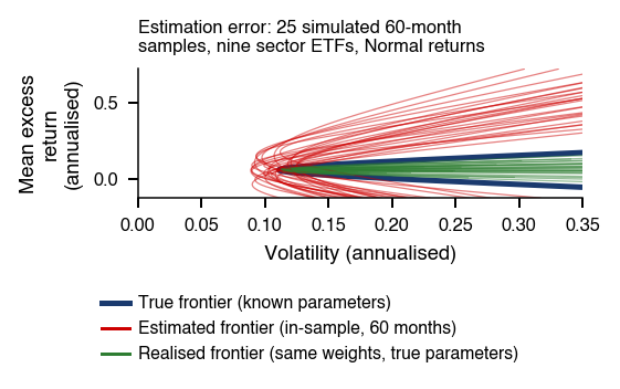
 MFM_ch4_two_asset




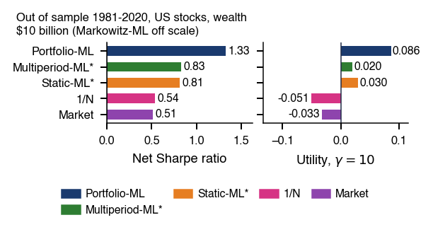
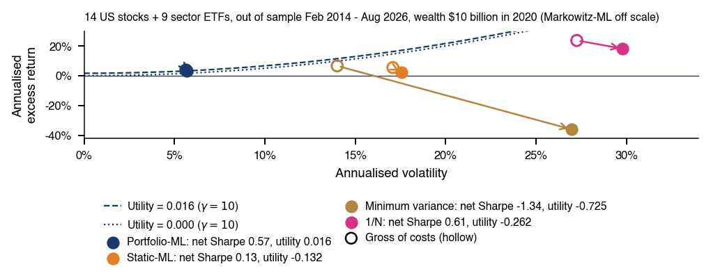
 Hierarchical Clustering