Bucharest University of Economic Studies IDA Institute Digital Assets Blockchain Research Center AI4EFin Artificial Intelligence for Energy Finance Romanian Academy, Institute for Economic Forecasting MSCA Digital Finance
“This paper shows that correlation coefficients are conditional on market volatility. Under certain assumptions, it is possible to adjust for this bias.” — Forbes & Rigobon (2002)
A 60/40 portfolio of two exchange-traded funds (ETFs): SPY (SPDR S&P 500 ETF Trust), on the S&P 500 (Standard & Poor's 500) index, and TLT (iShares 20+ Year Treasury Bond ETF), on US (United States) Treasury bonds with maturities above 20 years
volatility 10.4% with the 2002–2021 correlation (\(-0.40\)), 13.2% with the 2022–2026 one (\(0.11\))
The 252-day SPY–TLT correlation was positive on 6% of days before 2022 and on 81% of days since January 2022
2008: the variance of 2-day S&P 500 returns was 7.5 times its calm-year level
with a constant \(\beta\), a calm-period correlation of 0.4 is then measured as 0.77
after the Forbes–Rigobon adjustment, neither the Euro Stoxx 50 nor the BET (Bucharest Exchange Trading, index) crisis rise remains significant (stationary bootstrap: \(p = 0.98\) and \(0.62\))
JPM (JPMorgan Chase & Co., NYSE ticker) and BAC (Bank of America Corporation, NYSE ticker): when JPM has one of its 5% worst days, BAC is in its own worst 5% about 61% of the time
This paper shows that correlation coefficients are conditional on market volatility. Under certain assumptions, it is possible to adjust for this bias.
For twenty years, when United States (US) stocks fell, long-term US Treasury bonds tended to rise. That is why a portfolio of 60% stocks and 40% bonds was calmer than either part on its own. In 2022 this link reversed: since then, the two have often fallen together.
The difference shows up directly in risk. With the 2002–2021 link, the 60/40 portfolio has an annual volatility of 10.4%. With the 2022–2026 link, the same portfolio has 13.2%. The risk of each asset is the same in both computations; only the way they move together has changed.
The computation uses two exchange-traded funds (ETFs) of the United States (US). SPY (SPDR S&P 500 ETF Trust, where SPDR stands for Standard & Poor's Depositary Receipts) tracks the S&P 500 (Standard & Poor's 500) index of 500 large US companies. TLT (iShares 20+ Year Treasury Bond ETF) holds US Treasury bonds with maturities above 20 years.
The chapter studies this joint movement, measured first of all by the correlation. It answers four questions:
How precisely can we measure a correlation from daily returns?
How do we track a correlation that changes from one day to the next?
Do correlations really rise in crises, or do they only seem to rise because markets become more turbulent?
What happens on extreme days, which the correlation does not describe well?
The last question has a clear example. When the bank JPMorgan Chase & Co. (stock ticker JPM) has one of its 5% worst days, Bank of America Corporation (stock ticker BAC) is also in its own worst 5% about 61% of the time. Large losses come together far more often than an ordinary correlation would suggest.
Compute a time-varying covariance: rolling window, exponentially weighted moving average (EWMA) and dynamic conditional correlation (DCC), built on GARCH (generalised autoregressive conditional heteroskedasticity) models.
Derive the delta-method standard error of a correlation.
Derive the volatility bias of crisis correlations and separate it from contagion.
Compute copula fits and goodness-of-fit tests.
Interpret tail dependence, at a finite threshold and in the limit.
AI for Scientific DiscoveryArtificial intelligence (AI) as a research assistant: will the stock–bond correlation stay positive? A mini-case on inflation.
SummaryThe decision checklist, self-checks and the practical decision.
Chapter 5 modelled the risk of a single asset. This chapter looks at several assets at once and asks how they move together. The object of study is the covariance matrix \(\Sigma\) of returns: the variances sit on the diagonal, the covariances off it, and the correlations are obtained from them.
Correlation matters in three situations: when we compute the risk of a portfolio, when we hedge a position and when we judge whether a crisis spreads from one market to another. In all three, the correlation is not observed directly. It is estimated from data and it changes over time.
When Do Markets Move Together, and How Sure Can We Be? (1/2)
The chapter uses results from three earlier chapters:
Chapter 1: daily returns have fat tails, and turbulent periods come in clusters. For this reason, the classical confidence interval for a correlation is too narrow.
Chapter 4: the covariance matrix \(\Sigma\) is the input of portfolio choice.
Chapter 5: the GARCH model (generalised autoregressive conditional heteroskedasticity) describes the changing volatility of a single asset.
The results here are used later for portfolio risk, Value-at-Risk (VaR) and Expected Shortfall (ES), in Chapter 7, for checking these measures (backtesting) in Chapter 8 and for systemic risk in Chapter 18. Detailed examples and advanced topics are in Further Topics, after the Summary.
Diversification reduces risk only if the assets do not move perfectly together (Markowitz, 1952). For two assets with weights \(w\) and \(1-w\), volatilities \(\sigma_1\),\(\sigma_2\) and correlation \(\rho\), the portfolio variance is
\[\sigma_p^2 = w^\top\Sigma w = w^2\sigma_1^2+(1-w)^2\sigma_2^2+2w(1-w)\rho\,\sigma_1\sigma_2 .\]
(6.1)
The correlation appears in a single term of (6.1), the last one. With positive weights, a higher correlation means a riskier portfolio. A negative correlation makes the term negative, so the two assets partly offset each other's losses.
The chapter's example uses two exchange-traded funds (ETFs): SPY, on the S&P 500 stock index, and TLT, on US Treasury bonds with maturities above 20 years. Over July 2002 – September 2026, the annual volatility is 18.8% for SPY and 14.3% for TLT.
A 60/40 portfolio of the two has a volatility of 10.4% if we use the 2002–2021 correlation, equal to \(-0.40\). With the 2022–2026 correlation, equal to \(0.11\), the volatility rises to 13.2%. The volatilities of the two funds are the same in both computations; only the correlation differs.
Splitting the sample in January 2022, at the start of the inflation shock, is a convention for the illustration. A formal test, presented in Further Topics, places the change earlier, in August 2020.
The second use of the correlation is hedging. We hold a position \(S\) and want to reduce its risk by selling another instrument \(F\), for example a futures contract. The question is how much of \(F\) to sell. The answer that makes the variance of the hedged position as small as possible is the minimum-variance hedge ratio:
\[h^* = \rho\,\frac{\sigma_S}{\sigma_F},\]
(6.2)
that is, the slope of the regression of the return \(r_S\) on the return \(r_F\). The ratio in (6.2) is in value: how many units of value of \(F\) per unit of value of \(S\). To obtain the number of contracts, multiply by \(P_S/P_F\), the ratio of the prices, contract size included.
With the optimal ratio, the hedge removes the share \(\rho^2\) of the variance: the larger the correlation in absolute value, the more risk the hedge removes. If the correlation changes, yesterday's ratio is no longer optimal today. A hedge that adjusts over time needs a correlation that adjusts over time, \(\rho_t\).
The third use concerns crises. Forbes & Rigobon (2002) call contagion a significant increase in the links between markets after a shock. Interdependence means the links that are always present, through trade, common investors or common macroeconomic factors. Correlations tend to rise exactly when diversification would be most useful. The chapter asks how much of this rise is genuine.
The three uses share one point, which is also the new idea of the chapter: the covariance matrix is not fixed. It takes a different value at each date \(t\), written \(\Sigma_t\).
In brief
Hedging
How much value of the hedge \(F\) to sell per unit of value held in the position \(S\) to minimise the variance
Minimum-variance hedge ratio \(h^*=\rho\,\sigma_S/\sigma_F\): the slope of the regression of \(r_S\) on \(r_F\). Estimated on returns, it is a ratio of values: units of \(F\) per unit of \(S\) are \(h^*P_S/P_F\) (\(P_S\), \(P_F\): prices, contract size included)
\(r_S\), \(r_F\): returns of the position and of the hedge
\(\sigma_S\), \(\sigma_F\): their volatilities
Effectiveness \(\rho^2\): the share of the variance removed
If the correlation moves, yesterday's hedge is wrong today: a dynamic hedge needs a dynamic \(\rho_t\)
The chart shows the correlation between daily SPY and TLT returns, computed on a window that moves through time. The band around it is the 95% Fisher confidence interval, built as if the days were independent and identically distributed (i.i.d.).
The first slider chooses the window length, from 63 to 756 trading days. The second chooses the last day of the window. The readout gives the correlation of the chosen window and its interval, and the ▶ button moves the window through the sample. The shaded bands mark three stress episodes: autumn 2008 – March 2009, February–April 2020 and January–October 2022.
Question for the room The SPY–TLT correlation turned positive from 2022. With positive weights and unchanged volatilities, what does this rise in correlation do to the variance of a SPY–TLT portfolio?
Answer
It raises it: the covariance term of portfolio variance is 2w₁w₂σ₁σ₂ρ, so with positive weights it increases with ρ. On the 252-day window the correlation was positive on 6% of the days before 2022 and on 81% of the days from January 2022, so bonds offset less of the equity losses. The explanation discussed in the lecture: growth shocks move stocks and bonds in opposite directions, inflation shocks move them in the same direction. The chart documents the change in correlation; by itself it does not identify the shock behind it.
On the 252-day window, that is one trading year, the correlation was positive on only 6% of the days before 2022. From January 2022, it was positive on 81% of the days. By (6.1), this change raises the risk of every SPY–TLT portfolio: bonds now offset little of the equity losses.
On the one-year window, the correlation fell as low as \(-0.77\) in August 2012 and rose as high as \(0.32\) in July 2024. For two decades, long-term bonds protected equity portfolios. Since 2022, they have mostly moved in the same direction as stocks.
A frequently discussed explanation is the type of shock that dominates the market. A growth shock moves stocks and bond prices in opposite directions: bad news lowers stocks and raises bonds. The correlation is then negative. An inflation shock hits both markets in the same direction, so the correlation turns positive, as in 2022. The chart shows the change but does not by itself prove which shock caused it; the AI section returns to this question.
The Fisher band in the chart is too narrow. It assumes Normally distributed returns, without fat tails and without clustered turbulent periods, and daily returns do not look like that. The next section computes an interval that takes these features into account and shows how much wider it is.
In brief
Daily SPY and TLT returns, 252-day window
band: 95% Fisher interval (defined in the next section) assuming i.i.d. (independent and identically distributed) data
shaded: autumn 2008 – March 2009, February–April 2020, January–October 2022
Values of the correlation
minimum: \(-0.77\) (8 August 2012)
maximum: \(0.32\) (1 July 2024)
last: \(0.24\) (18 September 2026)
Positive correlation
on 6% of days before 2022
on 81% of days since January 2022
The sign depends on the type of shock
growth shocks move stocks and bond prices in opposite directions (negative correlation)
inflation shocks hit both (positive, as in 2022)
The Fisher band is too narrow here
it ignores fat tails and volatility clustering (next section)
Type of evidence: description (it shows what happened in the data, without testing a cause)
Correlation enters portfolio risk through a single term, the hedge ratio through (6.2) and the contagion question through its rise in crises. For SPY and TLT, it was negative for two decades and has been mostly positive since 2022. Two questions follow: how precisely can we estimate a correlation, and how do we model a covariance matrix that changes?
Measuring Covariance and Its Uncertainty
Before modelling a covariance matrix that changes over time, we need to know how to measure it. This section shows why the daily correlation between distant markets comes out too low, how large the error of an estimated correlation is, and how to estimate today's correlation from recent days.
Estimating \(\Sigma\) and its uncertainty has three traps:
Closing times differ from one market to another, so the measured correlation depends on the frequency of the data.
Daily returns have fat tails, and turbulent periods come in clusters (volatility clustering). Both features change the uncertainty of the estimate, and the classical interval ignores them.
The length of the estimation period decides how quickly we notice a change of regime.
In brief
The question of this section: how do we estimate \(\Sigma\), and how uncertain is each estimated correlation?
First trap: closing times differ, so the data frequency changes the correlation
Second trap: fat tails and volatility clustering can change the uncertainty substantially, and the Fisher interval ignores them
Third trap: the window length decides how fast we see a regime change
Asynchronous Trading and the Bias of Daily Correlations
The Bucharest Stock Exchange and the euro-area exchanges close several hours before the New York exchange. A US news item released after the European close enters European prices only the next day. This lag is called asynchronous trading.
When two markets generally move in the same direction, the lag has two effects. The same-day correlation comes out lower than the true link. The lagged correlation, between the US yesterday and Europe today, comes out positive, because part of the European reaction arrives one day late.
There are two remedies:
Use returns over longer periods, 2-day or weekly. Over a longer period, a one-day delay matters less.
Add the lagged correlation to the same-day one: \(\rho_0+\rho_{+1}\). Here \(\rho_0\) is the same-day correlation and \(\rho_{+1}\) the correlation between yesterday's US returns and today's European returns. The sum is only a rough approximation. It assumes a one-day lag, no autocorrelation and equal variances.
The rule used throughout the chapter: first align prices on the days when both exchanges traded, and only then compute returns.
In brief
Closing times differ
the Bucharest Stock Exchange and the euro-area exchanges close hours before New York
US news after the European close enters European prices only the next day
Consequence, under positive dependence (as between equity markets)
the same-day correlation is biased towards zero
the lagged correlation is positive
Remedies
Lower frequency: 2-day or weekly returns on common trading days
Add the lead–lag term: \(\rho_{0}+\rho_{+1}\) (\(\rho_0\): same-day correlation, \(\rho_{+1}\): US yesterday with Europe today)
The sum \(\rho_0+\rho_{+1}\) is a rough approximation of the synchronous correlation, valid only for a one-day lag, no autocorrelation and equal variances
Rule used throughout
first align the prices on common trading days
then compute returns
Daily, 2-Day and Weekly Correlations, 2000–2026 (1/2)
The chart compares the correlations between SPY, the Euro Stoxx 50 and the BET, the main index of the Bucharest Stock Exchange. Each correlation is computed at three frequencies: daily, \(k\)-day and weekly returns. The bars carry 95% Fisher confidence intervals.
The slider sets the horizon \(k\) of the middle returns, from 1 to 20 days, and the ▶ button increases it. The result box gives the correlation of each pair at the three frequencies and the lagged correlations.
Question for the room The daily SPY–Euro Stoxx 50 correlation is 0.59. Why does it rise to 0.79 on weekly returns?
Answer
Euro-area exchanges close before New York, so US news released after the European close enters European prices only the next day. The same-day correlation is biased towards zero, and the lagged correlation (SPY yesterday, Euro Stoxx 50 today) is 0.20. Over longer horizons the one-day lag matters less and less.
The same-day SPY–Euro Stoxx 50 correlation is 0.59 and rises with the horizon. On longer returns, the one-day delay of European prices matters less and less. The lagged correlation, SPY yesterday with the Euro Stoxx 50 today, is 0.20: part of the link appears only the next day.
For SPY and the Euro Stoxx 50, the correlation rises from 0.59 on daily returns to 0.71 on 2-day returns and 0.79 on weekly returns. For SPY and the BET, it rises from 0.22 daily to 0.38 weekly. The Euro Stoxx 50 and the BET close at almost the same time, and their correlation changes less, from 0.33 to 0.41.
The rise is largest for the pairs that close at different times, which confirms the explanation. Weekly data have a cost, though: they give 1,367 observations instead of 6,446, so the confidence intervals are wider. The choice of frequency is a trade-off: less bias or more precision.
In brief
SPY, Euro Stoxx 50 and BET on common trading days
BET: the main index of the Bucharest Stock Exchange
vertical lines on the bars: 95% Fisher intervals
SPY–Euro Stoxx 50 correlation
\(0.59\) daily, \(0.71\) on 2-day returns, \(0.79\) weekly
SPY yesterday with Euro Stoxx 50 today: \(0.20\)
SPY–BET correlation
\(0.22\) daily versus \(0.38\) weekly (lagged \(0.17\))
Euro Stoxx 50–BET, almost synchronous closes
\(0.33\) versus \(0.41\)
Weekly data are cleaner
but give \(1\,367\) instead of \(6\,446\) observations: wider intervals
Type of evidence: comparison of procedures (it shows which method works better on the same data, not why)
All returns in the chapter are log returns, \(r_t=\ln P_t-\ln P_{t-1}\), computed after aligning prices on common trading days. Each application uses the frequency that suits its purpose:
Daily returns serve where speed of reaction matters: the dynamic correlation model, confidence intervals and hedging.
2-day returns serve for the tests of crisis correlations, because they absorb the differences in closing times. In those tests, two consecutive 2-day returns share a day, and inference must account for this overlap. In the three-frequency chart, the 2-day returns do not overlap.
Weekly returns, computed from Friday closes, serve for the applications that combine many time zones: correlations on extreme days, market integration and bank networks. They reduce the bias but give fewer observations.
In brief
Returns are log returns, \(r_t=\ln P_t-\ln P_{t-1}\)
computed after aligning the prices on common trading days
Daily: DCC, HAC intervals and hedging, where the reaction speed matters
HAC: standard errors robust to heteroskedasticity and autocorrelation, defined below
2-day: the Forbes–Rigobon tests, to absorb different closing times
in these tests 2-day returns overlap: two consecutive returns share one day
in the three-frequency chart they do not overlap
Weekly (Friday closes): exceedance correlations, market integration and bank networks
applications of the copula and applications sections, which mix time zones
Sample Covariance and Inference on a Correlation (1/2): Estimator and Fisher Interval
Let \(r_t\in\mathbb{R}^N\) be the vector of the \(N\) returns on day \(t\),\(t=1,\dots,T\), and \(\bar r\) the vector of means. The sample covariance matrix and the Pearson correlation of assets \(i\) and \(j\) are
The matrix has \(N(N+1)/2\) distinct elements. For \(N=500\) assets, that means 125,250 quantities to estimate: their number grows with the square of the number of assets.
How reliable is a single estimated correlation? The classical answer uses the Fisher transformation, \(z=\operatorname{artanh}\hat\rho=\tfrac12\ln\frac{1+\hat\rho}{1-\hat\rho}\). It puts the correlation on a scale on which the error has roughly the same size, whatever \(\rho\) is. If days are independent and returns are Normal,
For one year of data, \(T=252\), and \(\rho=0.5\), the interval (6.3) has a half-width of about \(0.09\). The interval is not symmetric around the estimated correlation, because the function \(\tanh\) compresses values close to \(\pm1\).
In brief
Sample covariance matrix and Pearson correlation of \(N\) assets over \(T\) days
Daily returns are neither independent nor Normal, so we need another formula for the error. The delta method writes the error of the estimated correlation as an average of daily contributions. With \(\tilde x_t\),\(\tilde y_t\) the two returns standardised to mean 0 and variance 1,
where \(\psi_t\) is the contribution of day \(t\) to the error. The standard error (SE) of the correlation comes from the variance of these contributions.
Two features of the data change this variance. Fat tails make the contributions more variable. Clustered turbulent periods make the contributions of nearby days depend on each other. The HAC (heteroskedasticity and autocorrelation consistent) estimator accounts for both (Newey & West, 1987). It adds up the covariances of contributions up to \(L\) days apart, with Bartlett weights. The usual rule \(L=\lfloor4(T/100)^{2/9}\rfloor\) gives \(L=9\) for \(T=4{,}891\) and \(L=4\) for a 252-day window.
For independent Normal data, the variance of the contributions is \((1-\rho^2)^2\), exactly the Fisher variance; the derivation is in the Appendix. The HAC standard error, however, requires finite fourth moments, and Chapter 1 casts doubt on this condition.
For SPY–TLT in 2002–2021, with \(T=4{,}891\) and \(\hat\rho=-0.403\), the standard error is 0.0120 by the Fisher formula. If we account only for fat tails (\(L=0\)), it rises to 0.0217. With HAC and \(L=9\), it is 0.0227. Almost all of the increase therefore comes from fat tails, not from dependence between days.
In brief
Delta method: linearise \(\hat\rho\), a smooth function of sample moments, and write the error \(\hat\rho-\rho\) as a mean of daily contributions \(\psi_t\)
The chart compares the two intervals along the SPY–TLT correlation computed on a moving window. The top panel shows the correlation with the Fisher interval and the HAC interval, both at 95%. The bottom panel shows how many times wider the HAC interval is than the Fisher interval.
The selector sets the window length: 126, 252 or 504 days. The slider sets the number of days \(L\) in the HAC estimator, from 0 to 20, and the ▶ button increases it. The result box gives the median and the 90% quantile of the width ratio and the share of windows in which each interval excludes zero.
Question for the room If we choose L = 0 (no lags), does the HAC interval for the SPY–TLT correlation coincide with the Fisher interval?
Answer
No. On the 252-day window, the median ratio of the HAC width to the Fisher width is 1.17 at L = 0, 1.24 at L = 4 and 1.39 at L = 20. The Fisher formula assumes i.i.d. pairs from the bivariate Normal distribution; L = 0 removes only the lagged terms, not the fourth moments in the standard error. Over 2002–2021 the standard error of the correlation is 0.0120 by Fisher and 0.0217 without lags. With L = 4, the conclusion of the test changes in 8.2% of the windows. The HAC interval itself needs finite fourth moments, which Chapter 1 puts in doubt: HAC handles the dependence but does not compensate for missing moments.
Even with \(L=0\), the two intervals do not coincide. On the 252-day window, the median width ratio is 1.17 at \(L=0\), 1.24 at \(L=4\) and 1.39 at \(L=20\). Fat tails alone widen the interval, and dependence between days widens it further.
On the 252-day window, with \(L=4\), the HAC interval is wider than the Fisher interval in 91% of windows. At the median, it is 1.24 times as wide.
The difference changes conclusions. The correlation appears significantly different from zero in 73% of windows by Fisher and in only 65% by HAC. These are window-by-window results, not a joint test.
Over whole periods, the HAC standard error is 1.9 times the Fisher one in 2002–2021 and 1.4 times since 2022. Accounting for fat tails alone, the ratio is already 1.8 in the first period and 1.28 in the second. Fat tails therefore matter more than dependence between days.
The rule for daily returns: report HAC intervals obtained by the delta method. They are valid only if fourth moments are finite, and the estimates of Chapter 1 cast doubt on this. HAC handles dependence over time, but it cannot repair missing moments.
In brief
252-day rolling correlation, every 5th day
the 95% Fisher interval
the 95% HAC delta-method interval (Bartlett, \(L=4\))
HAC is wider than Fisher in 91% of windows and narrower in 9%
width ratio: median \(1.24\), 90% quantile \(1.54\)
Correlation significantly different from zero
73% of windows by Fisher, 65% by HAC
the verdict flips in 8.2%
pointwise results, window by window, not a simultaneous test
Whole periods: HAC SE \(=1.9\times\) Fisher in 2002–2021, \(1.4\times\) since 2022
fourth moments alone give \(1.8\times\) in 2002–2021 (\(1.28\times\) since 2022)
fat tails matter more than autocorrelation
Rule for daily returns: report delta-method HAC intervals
valid under stationarity and weak dependence
and only if fourth moments are finite, which the Hill estimates of Chapter 1 put in doubt
HAC handles the dependence but does not compensate for missing moments
How do we estimate today's covariance matrix? The simplest answer uses the last \(m\) days, with equal weights. With the mean set to zero, as is usual for daily data,
where \(r_s\) is the vector of returns on day \(s\). This estimator never gives a portfolio a negative variance: for any weight vector \(v\),\(v^\top\hat\Sigma_tv=\frac1m\sum_s(v^\top r_s)^2\ge0\). The matrix is singular, however, whenever the window has fewer days than assets, \(m<N\).
Equal weights have a defect called the ghost effect. An extreme day stays in the estimate with the same weight for \(m\) days, then drops out abruptly, and the estimate jumps although the market has not changed. The window length sets a trade-off. A short window reacts fast but is noisy. A long one is stable but notices a change of regime late.
In brief
Rolling window of length \(m\): \(\hat\Sigma_t=\frac1m\sum_{s=t-m}^{t-1} r_s r_s^\top\)
mean set to zero for daily data
\(r_s\): return vector of day \(s\)
\(m\): number of past days used
Positive semidefinite
for any weight vector \(v\), \(v^\top\hat\Sigma_tv=\frac1m\sum_s(v^\top r_s)^2\ge0\)
so every portfolio variance is \(\geq0\)
Singular if \(m<N\)
positive definite only if the \(m\) return vectors span \(\R^N\)
a singular matrix cannot be inverted, so it gives no minimum-variance weights
Ghost effect: an extreme day enters with weight \(1/m\) and leaves abruptly \(m\) days later
the estimate then jumps although the market has not changed
The trade-off
a short window reacts fast but is noisy
a long one is stable but detects a regime change late
The exponentially weighted moving average (EWMA), used in RiskMetrics (J.P. Morgan/Reuters, 1996), replaces the equal weights. Each day counts slightly less than the day after it:
where \(\lambda\in(0,1)\) is the decay factor. The observation from \(k\) days ago has weight \((1-\lambda)\lambda^{k-1}\). The usual values are \(\lambda=0.94\) for daily data and \(\lambda=0.97\) for monthly data. With \(\lambda=0.94\), the weights halve every 11.2 days, and the estimate effectively uses about 32 days.
Because the weights decline gradually, EWMA has no ghost effect. Its limitations: a single \(\lambda\) governs all variances and covariances, and the estimate does not revert to a long-run mean: (6.6) is an integrated GARCH(1,1) without a constant (Chapter 5). The factor \(\lambda\) plays the role of the window length \(m\), with the same trade-off between speed and noise.
The chart shows the SPY–TLT correlation since 2019, estimated by EWMA and by a moving window, with a 250-day window as reference. The first slider sets the decay factor \(\lambda\), from 0.8 to 0.995. The second sets the window length \(m\), from 20 to 500 days. The ▶ button increases \(\lambda\).
The result box shows how fast and how noisily each estimator reacts: the half-life and effective sample of EWMA, the daily variation of the estimate and the date on which the positive correlation of 2022 is confirmed (the 20th consecutive day of positive correlation).
Question for the room When ▶ raises λ from 0.94 towards 0.995, how does the date on which EWMA confirms the positive correlation of 2022 move?
Answer
Later: the 20th consecutive day of positive correlation is 10 May 2022 at λ = 0.94 (the run begins on 12 April) and 9 December 2022 at λ = 0.995, after the 250-day window (8 December). The weight on the most recent return product is 1 − λ: 6% at λ = 0.94 and 0.5% at λ = 0.995; the half-life of the weights rises from 11.2 to 138.3 days. Speed has a price: the standard deviation of the daily change of the correlation is 0.060 at λ = 0.94, 0.007 at λ = 0.995 and 0.0088 for the 250-day window.
A larger \(\lambda\) gives a later signal. At \(\lambda=0.94\), the positive correlation of 2022 is confirmed on 10 May. At \(\lambda=0.995\), it is confirmed only on 9 December 2022, almost together with the 250-day window, which confirms it on 8 December. The reason: the most recent day has weight \(1-\lambda\), that is 6% at \(\lambda=0.94\) and only 0.5% at \(\lambda=0.995\).
Speed is paid for with noise. The daily change of the estimated correlation has standard deviation 0.060 for EWMA with \(\lambda=0.94\) and only 0.0088 for the 250-day window. For both estimators, \(\lambda\) and \(m\) are chosen by the analyst, not estimated from the data. The model of the next section estimates from the data how fast the correlation reacts and how long it remembers the past.
In brief
Two EWMA estimators (\(\lambda=0.94\) and \(0.97\)) and two rolling windows (60 and 250 days)
Noise: standard deviation of the daily change of the estimate
0.060 (EWMA 0.94)
0.032 (EWMA 0.97)
0.0088 (250-day window)
Regime signal: 20 positive days in a row
EWMA (\(\lambda=0.94\)): began on 12 April 2022, confirmed on 10 May
250-day window: began on 10 November, confirmed only on 8 December 2022
With EWMA and rolling windows, \(\lambda\) and \(m\) are chosen by the analyst, not estimated
DCC (next section) estimates the reaction speed and the memory of the correlation from the data
Daily correlations between markets in different time zones come out too low. Returns over longer periods correct the bias but give fewer observations. On daily returns, the Fisher interval is too narrow, mostly because of fat tails; the HAC interval by the delta method is the default choice, provided fourth moments are finite. Moving windows and EWMA estimate today's covariance, but their speed of reaction is chosen by the analyst. The next section estimates it from the data.
Multivariate GARCH and DCC
This section builds a model in which the covariance matrix changes every day by a rule estimated from the data. The GARCH model of Chapter 5 extends directly to a matrix, but two problems appear: the number of parameters explodes, and the resulting matrix can give some portfolios a negative variance.
The DCC (dynamic conditional correlation) model of Engle (2002) solves both problems. Its idea is to separate the volatilities from the correlations. Each asset has its own GARCH model for volatility, and all correlations are driven by only two parameters.
From Univariate to Multivariate Volatility (1/2): the Model
In Chapter 5, the return of a single asset was \(r_t=\sigma_t z_t\), with \(\sigma_t^2=\omega+\alpha r_{t-1}^2+\beta\sigma_{t-1}^2\). With \(N\) assets, the volatility \(\sigma_t\) becomes a covariance matrix \(H_t\), and the vector of returns is written
so that \(\operatorname{Var}(r_t\mid\mathcal F_{t-1})=H_t\). Here \(z_t\) are the standardised shocks, \(\mathcal F_{t-1}\) is the information available up to yesterday, and \(I_N\) is the identity matrix. \(H_t\) is the \(\Sigma_t\) of the previous section, and \(H_t^{1/2}\) is a square root of it: \(H_t^{1/2}(H_t^{1/2})^\top=H_t\).
A good model for \(H_t\) must meet three requirements:
\(H_t\) is positive definite at every \(t\), so every portfolio has a positive variance.
The number of parameters stays small.
The parameters have a clear interpretation.
The parameters are estimated by maximising the Gaussian quasi-log-likelihood:
where \(|H_t|\) is the determinant of \(H_t\). The prefix "quasi" says that the Normal formula can be used even when the shocks are not Normal: the estimates remain consistent if the model for \(H_t\) is correct.
In brief
The question of this section: how do we model a covariance matrix that changes every day?
the matrix must stay positive definite and have few parameters
Chapter 5: one asset, \(r_t=\sigma_t z_t\), \(\sigma_t^2=\omega+\alpha r_{t-1}^2+\beta\sigma_{t-1}^2\)
The most general extension of GARCH is the VEC model (vectorised multivariate GARCH, built on the vech operator, which stacks the distinct elements of the covariance matrix in a vector) of Bollerslev, Engle & Wooldridge (1988). In it, every variance and covariance of today can depend on all products of yesterday's returns and on all elements of \(H_{t-1}\). The \(\operatorname{vech}\) operator stacks the \(N(N+1)/2\) distinct elements of a symmetric matrix into a vector:
The number of parameters grows as \(N^4\), and nothing guarantees that \(H_t\) stays positive definite.
The BEKK (Baba–Engle–Kraft–Kroner) model of Engle & Kroner (1995) writes \(H_t=CC^\top+A^\top r_{t-1}r_{t-1}^\top A+B^\top H_{t-1}B\), with \(C\) lower triangular and \(A\),\(B\) of size \(N\times N\). Each term is a quadratic form, so \(H_t\) is positive definite by construction. The parameters still grow as \(N^2\), however, and the elements of \(A\) and \(B\) are hard to interpret.
The table on the slide counts the parameters. For \(N=2\) assets, VEC has 21, full BEKK 11 and DCC \(6+2\). For \(N=50\), VEC has 3,252,525, BEKK 6,275 and DCC only \(150+2\). DCC uses three GARCH parameters per asset, so \(3N\), plus the two correlation parameters \(a\) and \(b\). For large portfolios, VEC and BEKK can no longer be estimated in practice.
parameters: 3 in \(c\), \(3\times3=9\) in \(A\) and 9 in \(B\), so 21 (the table on the previous slide)
the general form \(\operatorname{vech}(H_t)=c+A\operatorname{vech}(r_{t-1}r_{t-1}^\top)+B\operatorname{vech}(H_{t-1})\) is exactly this system, written in matrix form
The problem: nothing prevents \(h_{12,t}^2>h_{11,t}h_{22,t}\), that is, a “correlation” above 1 in absolute value
The idea: a variance cannot be negative if we write it as a square
univariate: \(\alpha r_{t-1}^2=(a\,r_{t-1})^2\) with \(a=\sqrt\alpha\), so the news term is always \(\ge0\)
BEKK does the same with matrices: \(A^\top r_{t-1}r_{t-1}^\top A=(A^\top r_{t-1})(A^\top r_{t-1})^\top\), the “square” of a vector
What \(A^\top r_{t-1}\) is: yesterday's shocks, mixed
asset 1 receives \(a_{11}r_{1,t-1}+a_{21}r_{2,t-1}\): its own shock plus part of the other asset's shock
with a diagonal \(A\) there is no mixing: each asset reacts only to its own shock
The square of a vector is always a valid covariance matrix
the diagonal holds squares (\(\ge0\)), and the “correlation” of this term is exactly \(+1\) or \(-1\), depending on the sign of \(r_{1,t-1}r_{2,t-1}\)
the same holds for \(B^\top H_{t-1}B\) (a transformation of a valid covariance) and for \(CC^\top\); a sum of valid covariances is valid
this is why \(H_t\) stays positive definite without any restriction on the parameters
What we get: \(H_t\) = a baseline level + the reaction to yesterday's news + the memory of \(H_{t-1}\)
the correlation in \(H_t\) combines the correlations of the three terms, weighted by each term's contribution to the variances: the news brings \(\pm1\), so days with same-sign shocks push it up
The price: \(A\) and \(B\) have \(N^2\) elements each, and one element does not describe a single variance or covariance
this is why the diagonal or scalar BEKK (\(A=a\,I_N\), \(B=b\,I_N\)), close in spirit to DCC, is used in practice
Compared with the diagonal VEC: the same form, but the covariance coefficients are no longer free
they are products of the coefficients of the two variance equations: \(a_{11}a_{22}\) instead of \(a_2\), \(b_{11}b_{22}\) instead of \(b_2\)
\(A^\top r_{t-1}r_{t-1}^\top A\) and \(B^\top H_{t-1}B\) are quadratic forms, hence positive semidefinite; with \(CC^\top\) positive definite, \(H_t\) stays positive definite at every \(t\)
7 parameters: 3 in \(C\) (lower triangular), 2 in \(A\), 2 in \(B\)
Full BEKK: \(A\), \(B\) arbitrary \(2\times2\) matrices, so \(3+4+4=11\) parameters
for example \(h_{11,t}\) contains \((a_{11}r_{1,t-1}+a_{21}r_{2,t-1})^2\): it also depends on \(r_{2,t-1}^2\) and on \(r_{1,t-1}r_{2,t-1}\)
this is why the elements of \(A\) and \(B\) have no direct interpretation
Here \(\sigma_{it}\) is the GARCH volatility of asset \(i\) and \(R_t\) is the correlation matrix. Dividing each return by its volatility gives the standardised residuals \(\varepsilon_{it}=r_{it}/\sigma_{it}\).
The simplest model, the constant conditional correlation (CCC) model of Bollerslev (1990), assumes that \(R_t=R\) does not change. The DCC model of Engle (2002) lets the correlations vary too. It applies a GARCH-type recursion to an auxiliary matrix \(Q_t\) and then turns it into a correlation matrix \(R_t\):
with \(a,b\ge0\) and \(a+b<1\). The parameters read as in GARCH. \(a\) measures how much the correlation reacts to yesterday's joint shocks, \(b\) how much it remembers of the past, and \(a+b\) how persistent it is. The second equation divides \(Q_t\) by its own diagonal, so that \(R_t\) has ones on the diagonal and is a valid correlation matrix.
The matrix \(\bar Q\) is the level to which the recursion reverts. It has \(N(N-1)/2\) free elements. In practice it is replaced by the sample covariance of the standardised residuals, \(\hat{\bar Q}=\frac1T\sum_t\varepsilon_t\varepsilon_t^\top\); this is called correlation targeting. Two parameters then drive all \(N(N-1)/2\) correlations. The model is very economical, but it imposes the same persistence on every pair of assets.
One subtlety matters further on: \(Q_t\) is not the expected correlation matrix. The expected correlation is \(R_t\), so \(\mathbb{E}_{t-1}[\varepsilon_t\varepsilon_t^\top]=R_t\ne Q_t\). The slide Two-Step Estimation (2/2) shows why this matters.
\(\bar Q\): the intercept matrix of the recursion, with \(N(N-1)/2\) free elements. Correlation targeting replaces it by the sample covariance \(\hat{\bar Q}=\frac1T\sum_t\varepsilon_t\varepsilon_t^\top\) (when this is consistent: slide “Two-Step Estimation (2/2)”)
\(a\): reaction to yesterday's product of shocks; \(b\): memory; \(a+b\): persistence, i.e. how slowly the correlation returns to the target
The second line rescales \(Q_t\) so that its diagonal is 1: \(R_t\) is a valid correlation matrix
Two parameters govern all \(N(N-1)/2\) correlations
parsimonious, but every pair has the same persistence
\(Q_t\) is a covariance proxy, not a correlation: \(\E_{t-1}[\varepsilon_t\varepsilon_t^\top]=R_t\ne Q_t\)
a day on which both assets fall (or rise) sharply pushes the correlation up, a day with opposite signs pushes it down; with a large \(b\), the effect fades slowly
In general (previous slide): the same recursions for all \(N(N-1)/2\) pairs, written as one matrix equation in \(Q_t\)
Two-Step Estimation (1/2): Splitting the Likelihood
Substitute \(H_t=D_tR_tD_t\) and \(\varepsilon_t=D_t^{-1}r_t\) into (6.7). The determinant factors as \(|H_t|=|D_t|^2|R_t|\), and the quadratic form becomes \(r_t^\top H_t^{-1}r_t=\varepsilon_t^\top R_t^{-1}\varepsilon_t\). Adding and subtracting \(\varepsilon_t^\top\varepsilon_t=r_t^\top D_t^{-2}r_t\), the likelihood splits in two:
The first part, \(\ell_V\), contains only the volatilities. Since \(D_t\) is diagonal, it is the sum of the \(N\) univariate GARCH log-likelihoods, \(\sum_i\big[-\tfrac12\sum_t(\ln2\pi+\ln\sigma_{it}^2+r_{it}^2/\sigma_{it}^2)\big]\). The second part, \(\ell_C\), depends on \((a,b)\) once the volatilities are given.
This gives the two-step estimator:
Step 1 estimates a separate GARCH(1,1) model for each asset and keeps the volatilities \(\sigma_{it}\) and the standardised residuals \(\varepsilon_{it}\).
Step 2 sets \(\bar Q\) to the sample covariance of the residuals and maximises \(\ell_C\) over \((a,b)\).
In brief
The Gaussian log-likelihood splits into a volatility part and a correlation part
Add and subtract \(\varepsilon_t^\top\varepsilon_t=r_t^\top D_t^{-2}r_t=\sum_i r_{it}^2/\sigma_{it}^2\): then \(\ell_V=\sum_i\big[-\tfrac12\sum_t(\ln2\pi+\ln\sigma_{it}^2+r_{it}^2/\sigma_{it}^2)\big]\), the sum of the \(N\) univariate Gaussian GARCH log-likelihoods
Step 1: fit \(N\) univariate GARCH(1,1) models, keep \(\sigma_{it}\) and \(\varepsilon_{it}\)
Step 2: fix \(\bar Q\) at the sample covariance of \(\varepsilon_t\) and maximise \(\ell_C\) over \((a,b)\)
The gain: instead of one joint maximisation, \(N\) univariate ones and one with two parameters; the cost: harder inference (next slide)
Two-Step Estimation (2/2): Targeting and Inference
Correlation targeting has a cost: the standard DCC estimator is, in general, inconsistent. The reason is the subtlety above. Taking expectations in (6.8), stationarity gives \((1-b)\,\mathbb{E}[Q_t]=(1-a-b)\,\bar Q+a\,\mathbb{E}[R_t]\). The sample covariance of the residuals estimates \(\mathbb{E}[R_t]\). It equals \(\bar Q\) only if \(\mathbb{E}[Q_t]=\mathbb{E}[R_t]\), and in general this equality fails, because \(R_t\) divides \(Q_t\) by a random diagonal.
The corrected DCC (cDCC) of Aielli (2013) fixes the problem. It uses \(\operatorname{diag}(Q_{t-1})^{1/2}\varepsilon_{t-1}\) in the recursion instead of \(\varepsilon_{t-1}\). Then \(\mathbb{E}[Q_t]=\bar Q\), and targeting becomes consistent.
The second difficulty concerns the standard errors. Those of step 2 treat the step-1 estimates and \(\bar Q\) as known exactly, so they ignore their uncertainty. There are two corrections: the sandwich matrix of two-step estimators (Newey & McFadden, 1994), given in the Appendix, and a bootstrap that redoes both steps, described there as well.
The third difficulty concerns the test. The CCC model is the case \(a=0\). Under the hypothesis \(H_0\colon a=0\), the parameter \(b\) has no effect and cannot be estimated. For this reason, the usual \(\chi^2\) distribution of the likelihood ratio (LR) test is only indicative. The chapter obtains the critical values from a bootstrap that simulates data under CCC.
In brief
Targeting with the sample covariance makes the standard DCC estimator inconsistent in general
why: take expectations of the recursion, using \(\E[\varepsilon_{t-1}\varepsilon_{t-1}^\top]=\E[R_{t-1}]\)
\(\hat{\bar Q}=\frac1T\sum_t\varepsilon_t\varepsilon_t^\top\) estimates \(\E[R_t]\), which equals the intercept \(\bar Q\) only if \(\E[Q_t]=\E[R_t]\)
That fails in general: \(R_t\) rescales \(Q_t\) by its own random diagonal
The corrected DCC of Aielli (2013) uses \(\operatorname{diag}(Q_{t-1})^{1/2}\varepsilon_{t-1}\) in place of \(\varepsilon_{t-1}\), so that \(\E[Q_t]=\bar Q\) and targeting remains consistent
Step-2 standard errors treat the GARCH estimates and \(\bar Q\) as known
propagate their error with the “sandwich” covariance matrix of both steps stacked together (Newey & McFadden (1994))
or by bootstrapping both steps: resample the data, re-estimate both steps and use the spread of the estimates (Appendix)
CCC against DCC: \(H_0: a=0\)
under \(H_0\), \(Q_t\) no longer depends on \(b\), so \(b\) is not identified and the \(\chi^2\) reference is only indicative
the p-value comes from a bootstrap: simulate data under CCC and re-estimate
The model is estimated on daily SPY and TLT returns, in percent, from 31 July 2002 to 18 September 2026, that is \(T=6{,}073\) days. In step 1, both volatilities are very persistent: \(\alpha+\beta\) is 0.975 for SPY and 0.993 for TLT. The average correlation of the standardised residuals, which serves as the target, is \(\hat{\bar Q}_{12}=-0.248\).
In step 2, \(\hat a=0.0522\) and \(\hat b=0.9335\). The persistence of the correlation is therefore \(a+b=0.986\): a shock to the correlation dies out slowly. A rough rule gives \(\ln0.5/\ln0.986\approx48\) days to halve it. It is not exact, because \(Q_t\) is not the expected correlation; the actual response of the correlation is obtained by simulation.
Is DCC better than a constant correlation? The LR test compares the likelihoods of the two models: \(LR=2(460.26-193.54)=533.4\). In 199 data sets simulated under CCC, the largest statistic obtained is only 15.7. The bootstrap \(p\)-value is therefore \(1/(B+1)=0.005\), the smallest possible with \(B=199\), and CCC is rejected. The slide also gives three standard errors for \(a\) and \(b\).
In brief
Step 1: GARCH(1,1), returns in %
\(\omega\)
\(\alpha\)
\(\beta\)
\(\alpha+\beta\)
SPY
0.0283
0.127
0.848
0.975
TLT
0.0057
0.049
0.943
0.993
Step 2: DCC(1,1) and three standard errors
estimate
Hessian
boot. step 2
boot. both
\(a\)
0.0522
0.0059
0.0051
0.0052
\(b\)
0.9335
0.0084
0.0077
0.0077
\(a+b\)
0.9857
–
0.0038
0.0040
Daily data 31 July 2002 – 18 September 2026, \(T=6\,073\)
target \(\hat{\bar Q}_{12}=-0.248\)
Persistence \(a+b=0.986\)
the heuristic measure \(\ln0.5/\ln0.986\approx48\) days, not the exact half-life of \(Q_t\)
\(\E_t[\varepsilon_{t+1}\varepsilon_{t+1}^\top]=R_{t+1}\ne Q_{t+1}\), so the deviation of \(Q\) does not decay exactly as \((a+b)^h\)
the actual response of the correlation comes from a conditional simulation
LR (Likelihood Ratio, test) test against CCC: \(LR=2(\hat\ell^{DCC}-\hat\ell^{CCC})=2(460.26-193.54)=533.4\)
bootstrap of both steps under CCC (\(B=199\)): the largest simulated value under \(H_0\) is \(15.7\)
so \(p=1/(B+1)=0.005\), the smallest attainable value: CCC is rejected
The three standard errors are close. Re-estimating the GARCH models in the bootstrap raises the dispersion of \(\hat a\) by only 2% and that of \(\hat b\) by 1%. With 199 replications, the simulation error of such a dispersion is about 5%, so the differences are within the noise. The result does not generalise: in other data, the uncertainty from step 1 can matter a lot.
TLT volatility is more persistent than that of SPY but reacts less to news, that is, it has a smaller \(\alpha\). The estimates here use the standard DCC and illustrate the method; with correlation targeting they are, in general, inconsistent, as shown in Two-Step Estimation (2/2).
In brief
In this bootstrap experiment, re-estimating GARCH raises the dispersion of \(\hat a\) by 2% and of \(\hat b\) by 1%
with \(B=199\), the Monte Carlo error of a bootstrap standard deviation is about 5%
here the step-1 uncertainty is therefore small, but the result is not general: the step-1 contribution can stay first-order as \(T\) grows
The Hessian SEs exceed the bootstrap standard deviations, which does not prove that their intervals cover the true value more often than the nominal level
The SPY–TLT correlation reacts little to a single day's shock (small \(a\)) but keeps its level for a long time (large \(b\))
TLT volatility is more persistent than SPY's (\(\alpha+\beta\): 0.993 versus 0.975)
but reacts less to news (smaller \(\alpha\))
These standard DCC estimates illustrate the method: with correlation targeting they are inconsistent in general (Two-Step Estimation (2/2))
The chart compares the DCC(1,1) correlation of SPY and TLT with the correlation over a 252-day moving window and with the target \(\hat{\bar Q}_{12}=-0.248\). The two sliders change the reaction \(a\) and the memory \(b\), starting at the estimated values. The path is recomputed from (6.8). The readout gives the persistence, the correlation part of the log-likelihood and the LR statistic against CCC.
Question for the room The DCC estimates are a = 0.052 and b = 0.934. What does their sum tell us?
Answer
It is the persistence of the correlation: a + b = 0.986; the heuristic measure ln 0.5 / ln(a + b) gives about 48 days, not the exact half-life of Q_t, since E_t[ε_{t+1}ε_{t+1}′] = R_{t+1}, not Q_{t+1}. The LR test against constant correlation gives 533.4; the bootstrap under CCC gives p = 0.005, the smallest possible value with B = 199. These are standard DCC estimates, an illustration of the method: with correlation targeting they are inconsistent in general.
The DCC correlation falls as low as \(-0.79\) in November 2011 and rises as high as \(0.49\) in May 2026. In 2022 its average is \(0.00\), against \(-0.56\) in 2012. Since January 2022 the path lies above the target on 92% of the days, against 36% before.
A single equilibrium correlation for the whole of 2002–2026 is therefore hard to defend. The break test in Further Topics dates the change of regime.
In brief
DCC(1,1) conditional correlation, the 252-day rolling correlation and the target \(\hat{\bar Q}_{12}=-0.248\)
The standard DCC path illustrates the method, subject to the targeting inconsistency (Two-Step Estimation (2/2))
Range \(-0.79\) (2 November 2011) to \(0.49\) (21 May 2026)
Last value \(0.36\)
Average DCC correlation
\(-0.54\) from 15 September to 31 December 2008
\(-0.56\) in 2012, \(0.00\) in 2022
Since January 2022 the path is above the target on 92% of days (36% before)
Does a dynamic correlation help build a portfolio? The application compares two daily minimum-variance SPY–TLT portfolios. Both use the same GARCH volatilities. One uses the DCC correlation, the other a constant correlation. The charts show the weight in SPY and the annualised volatility. The slider chooses the constant correlation, starting at the full-sample value, and the ▶ button changes it automatically.
Question for the room The in-sample volatility of the minimum-variance portfolio is 9.06% with DCC and 9.10% with GARCH and a constant correlation. What can we conclude about out-of-sample performance?
Answer
Nothing, from this comparison alone. The difference is about 0.04 percentage points of annualised volatility, and the parameters are estimated on the full sample: the result is neither an out-of-sample evaluation nor an equivalence test. The fixed 60/40 portfolio has 10.99%, so most of the gain comes from the GARCH volatilities. The DCC weights differ from the constant-correlation weights by 1.9 percentage points on average and by at most 22 (8 June 2026). ▶ changes the constant correlation: at 0.90 the constant-correlation volatility rises to 12.73%.
The two portfolios have almost the same risk: 9.06% with DCC and 9.10% with the constant correlation. The fixed 60/40 portfolio has 10.99%. Almost all of the gain comes from the GARCH volatilities. A wrong constant correlation is costly, though: with 0.90, the volatility rises to 12.73%. The comparison uses parameters estimated on the full sample, so it is not an out-of-sample evaluation.
truncated to \([0,1]\), where \(\sigma_{12,t}\) is the conditional covariance. The constant-correlation variant uses the full-sample 2002–2026 correlation, equal to \(-0.30\).
The weights of the two variants differ little: by 0.019 on average and by at most 0.22. DCC adds little beyond the GARCH volatilities. A fair test re-estimates the model on windows that expand over time and includes transaction costs (Chapter 4). Out-of-sample evaluation is the subject of Chapter 8, and the out-of-sample hedge in Further Topics gives a first example.
In brief
Weight in SPY of the daily minimum-variance SPY–TLT portfolio
\(w_t=(\sigma_{2t}^2-\sigma_{12,t})/(\sigma_{1t}^2+\sigma_{2t}^2-2\sigma_{12,t})\), truncated to \([0,1]\) (no short sales)
\(\sigma_{12,t}=\rho_t\sigma_{1t}\sigma_{2t}\): the conditional covariance
Same GARCH volatilities, correlation from DCC or constant
the constant one equals the full-sample 2002–2026 return correlation (\(-0.30\))
Annualised volatility
60/40 fixed: 10.99%
GARCH with constant correlation: 9.10%
GARCH with DCC: 9.06%
Most of the gain comes from GARCH volatilities, DCC adds little
the DCC and constant-correlation weights differ by 0.019 on average, by at most 0.22 (8 June 2026)
In-sample illustration: the parameters are estimated on the same data used for the evaluation
a fair test re-estimates on expanding windows and adds transaction costs (Chapter 4)
DCC separates the volatilities, modelled asset by asset with GARCH, from the correlations, driven by only two parameters. The split (6.9) of the likelihood gives the two-step estimator. With correlation targeting, the standard estimator is in general inconsistent, and the corrected DCC of Aielli (2013) fixes the problem. For SPY and TLT, the correlation is persistent (\(a+b=0.986\)) and CCC is rejected. In a minimum-variance portfolio, however, almost all of the gain comes from the volatilities. The question of the motivation remains: how much of the rise in correlations during crises is real?
Crisis Correlations and the Forbes–Rigobon Bias
Correlations measured during crises are usually higher than in calm periods. This section asks whether the link between markets has changed, or whether only the market where the crisis started has become more turbulent. Forbes & Rigobon (2002) show how to separate the two explanations.
A high crisis correlation must be compared with the calm one, and even a rise has two explanations. The first is contagion: the mechanism by which one market affects another changes. The second is the volatility bias: the mechanism stays the same, but the source market becomes much more volatile.
After correcting this bias, Forbes & Rigobon (2002) find that most of the apparent contagion in the 1987, 1994 and 1997 crises is in fact interdependence, the ordinary link between markets. A related finding concerns asymmetry. Longin & Solnik (2001) and Ang & Chen (2002) find that correlations rise in falling markets (bear markets) but not in rising ones (bull markets). The Normal distribution cannot produce such an asymmetry. The photograph shows the headquarters of Lehman Brothers in New York on 15 September 2008, the day of the bankruptcy filing.
The idea can be seen without formulas. A market's return has a part that comes from the source market and a part of its own, the local noise. The correlation measures how much of the movement comes from the common part. If the source market becomes more turbulent, the common part grows and the local noise does not. The correlation rises, although the link has not changed.
Formally, let \(x_t\) be the return of the source market and \(y_t\) the return of the other market:
The constant \(\beta\) measures how much is transmitted from \(x\) to \(y\). The own shock \(\varepsilon_t\) has constant variance \(\sigma_\varepsilon^2\), and \(\sigma_x^2\) is the variance of the source market. Because \(\varepsilon_t\) is uncorrelated with \(x_t\),\(\operatorname{Cov}(x_t,y_t)=\beta\sigma_x^2\) and \(\operatorname{Var}(y_t)=\beta^2\sigma_x^2+\sigma_\varepsilon^2\).
The ratio \(k\) compares the part transmitted from the source market with the own noise; it is called the signal-to-noise ratio. Equivalently, \(k=\rho^2/(1-\rho^2)\).(6.10) shows that the variance of the source market affects the correlation only through \(k\). And \(k\) rises with \(\sigma_x^2\) even when \(\beta\) does not change.
In brief
Model: \(y_t=\alpha+\beta x_t+\varepsilon_t\), \(\Cov(x_t,\varepsilon_t)=0\), \(\beta\) and \(\sigma_\varepsilon^2\) constant
\(x_t\): return of the source market
\(y_t\): return of the other market
\(\beta\): transmission coefficient
\(\varepsilon_t\): own shock of \(y\), variance \(\sigma_\varepsilon^2\)
\(\sigma_x^2\): variance of \(x\)
Two moments of the model
\(\Cov(x_t,y_t)=\beta\sigma_x^2\) and \(\Var(y_t)=\beta^2\sigma_x^2+\sigma_\varepsilon^2\), because \(\varepsilon_t\) is uncorrelated with \(x_t\)
In a crisis, denoted by the subscript \(c\), the only change is that the variance of the source market rises: \(\sigma_{x,c}^2=(1+\delta)\,\sigma_x^2\), with \(\delta>0\) the relative increase. Then \(k_c=(1+\delta)k\), and (6.10) gives \(\rho_c^2=(1+\delta)\rho^2/(1+\delta\rho^2)\). The correlation measured in the crisis follows:
For \(0<|\rho|<1\),\(|\rho_c|>|\rho|\): the measured correlation rises, although \(\beta\) is the same. Inverting the formula gives the crisis correlation adjusted for volatility,
An example: take a calm correlation \(\rho=0.5\) and a source variance that doubles (\(\delta=1\)). Then \(k=1/3\),\(k_c=2/3\) and \(\rho_c^2=0.4\), so \(\rho_c=0.632\). The correlation has risen by \(0.13\) with no change in \(\beta\).(6.12) gives back \(0.632/\sqrt{1+1\cdot(1-0.4)}=0.5\), the calm value.
The chart shows the crisis correlation \(\rho_c\) of (6.11) as a function of \(\delta\), for three calm correlations, with \(\beta\) held constant. The vertical line marks the 2008 crisis: the variance of 2-day S&P 500 returns was then 7.5 times its calm-year level, that is \(\delta=6.54\). The first slider sets \(\delta\), from 0 to 10, and the second the calm correlation. The ▶ button increases \(\delta\).
Question for the room In the 2008 crisis the variance of 2-day S&P 500 returns rose 7.5 times (δ = 6.54); with β unchanged, an unconditional correlation of 0.4 is measured in the crisis as 0.77. What happens to this measured correlation when ▶ raises δ to 10?
Answer
It keeps rising, ever more slowly: 0.82 at δ = 10. From ρ_c = ρ√((1 + δ)/(1 + δρ²)), the measured correlation approaches 1 only as δ → ∞. The higher variance of the source market raises the share of the common factor in the variance of the target market, although the transmission coefficient β and the variance of the idiosyncratic shock stay the same. At δ = 6.54, an unconditional correlation of 0.2 is measured as 0.49.
At \(\delta=6.54\), a calm correlation of 0.4 is measured as 0.77 in the crisis. A calm correlation of 0.2 becomes 0.49. As \(\delta\) grows further, the measured correlation keeps rising, ever more slowly; it approaches 1 only as \(\delta\to\infty\).
In brief
Measured crisis correlation \(\rho_c\) as a function of \(\delta\), for three calm-period correlations
\(\beta\) is constant: only the volatility of the source market rises
Vertical line: the 2008 crisis window
the variance of 2-day S&P 500 returns was \(7.5\) times its calm-year level (\(\delta=6.54\))
At this \(\delta\) a calm-period correlation of \(0.4\) is measured as \(0.77\) in the crisis
and \(0.2\) as \(0.49\)
For an investor: a crisis rise in correlation of this size does not by itself prove contagion
The test asks whether the crisis correlation, net of volatility, exceeds the calm one. It has four steps:
Choose the source market \(x\), a calm window and a crisis window.
Use 2-day returns, to absorb the different closing times.
Compute the rise in variance, \(\delta=\hat\sigma^2_{x,c}/\hat\sigma^2_{x,calm}-1\), and the adjusted correlation \(\rho^*\) of (6.12).
Test \(H_0\colon\rho^*\le\rho_{calm}\) with Fisher \(z\) statistics, as in Forbes & Rigobon (2002).
The Fisher test has two problems here: it treats \(\delta\) as a known number although it is estimated, and the 2-day returns overlap. With \(\delta\) fixed, \(\operatorname{Var}(\operatorname{artanh}\rho^*)\approx1/[n_c(1+\delta(1-\rho_c^2))]<1/n_c\), where \(n_c\) is the number of crisis days, so the Fisher test is conservative.
For both problems, the chapter uses a stationary bootstrap: samples built from blocks of consecutive days of random length, which keep the dependence between neighbouring days. The mean block length is 10 days, and the number of samples is \(B=1{,}999\). The calm and crisis windows are resampled jointly, and the test looks at the difference \(D=\rho^*-\rho_{calm}\).
The adjustment holds only under three assumptions:
There is no omitted common shock. A global factor that hits both markets raises \(\sigma_\varepsilon\) as well, not only \(\sigma_x\); the adjustment then over-corrects (Corsetti, Pericoli & Sbracia, 2005).
The market \(y\) does not feed back into the source market \(x\).
The variance of the own noise, \(\sigma_\varepsilon^2\), is the same in the two periods.
The choice of windows matters too: the conclusion can flip when the windows move by a few weeks.
In brief
Procedure
Choose the source market \(x\), a calm window and a crisis window
Use 2-day returns (closing times differ)
Compute \(\delta=\hat\sigma^2_{x,c}/\hat\sigma^2_{x,calm}-1\) and \(\rho^*\)
Test \(H_0: \rho^*\le\rho_{calm}\) (no contagion) with Fisher \(z\) statistics, the convention of Forbes & Rigobon (2002)
Inference
With \(\delta\) fixed, \(\Var(\operatorname{artanh}\rho^*)\approx1/[n_c(1+\delta(1-\rho_c^2))]<1/n_c\) (\(n_c\): crisis observations): the Fisher test is conservative (it rejects \(H_0\) too rarely)
But \(\delta\) is estimated and 2-day returns overlap: use a stationary bootstrap of the calm and crisis windows, resampled jointly, and test \(D=\rho^*-\rho_{calm}\)
Stationary bootstrap: resamples blocks of consecutive days (random starts, geometric lengths, mean 10 days; \(B=1\,999\) draws), keeping the serial dependence inside each block
Assumptions to remember
No omitted common shock
a global factor hitting both markets raises \(\sigma_\varepsilon\) as well as \(\sigma_x\)
The application takes the S&P 500 as the source and compares 2-day correlations with the Euro Stoxx 50 and the BET: in the calm year, in the crisis (raw) and in the crisis after the Forbes–Rigobon adjustment. The slider shifts both windows by up to eight weeks forward or back. The readout reports the three correlations and the \(p\)-values of the raw and the adjusted rise. The step-by-step computation is in Further Topics.
Both raw rises are significant at 5%, but neither survives the adjustment. For the Euro Stoxx 50, the bootstrap \(p\)-value of the adjusted rise is 0.98. For the BET, it is 0.62. The uncertainty about \(\delta\) is large: its 90% bootstrap interval is \([3.9, 9.6]\).
Under these assumptions, there is no evidence of contagion after the adjustment. This does not prove its absence: a large \(p\)-value is not the probability of the null hypothesis, and the test has low power. Moreover, in 2008 a global shock hit every market, so the adjustment may over-correct (Corsetti, Pericoli & Sbracia, 2005).
Question for the room After the Forbes–Rigobon adjustment, the one-sided test of a rise in the S&P 500–Euro Stoxx 50 correlation gives p = 0.93. What conclusion does it support?
Answer
We find no evidence of contagion, under the model’s assumptions: we do not reject the hypothesis that the adjusted correlation did not rise. The correlation is 0.61 in the calm year, 0.80 in the crisis (the raw rise has p = 0.005) and 0.44 after the adjustment. p = 0.93 comes from the one-sided Fisher z test computed on the page; the lecture’s stationary bootstrap gives p = 0.98. A large p-value is not the probability of the null hypothesis and does not prove the absence of contagion. For the BET, 0.48 becomes 0.20 (p = 0.55). The numbers change when the windows are shifted (▶), so their choice has to be justified.
For the Euro Stoxx 50, the correlation is 0.61 in the calm year and 0.80 in the crisis, and the raw rise has \(p=0.005\). After the adjustment, the crisis correlation falls to 0.44. The Fisher \(z\) test computed on the page gives \(p=0.93\) for the adjusted rise. For the BET, the crisis correlation of 0.48 becomes 0.20 after the adjustment. The numbers change when the windows move, so the windows have to be justified in advance.
Section summary
A more volatile source market raises the measured correlation on its own, as (6.11) shows. (6.12) removes this effect. In 2008 the raw rises of the S&P 500 correlations with the Euro Stoxx 50 and the BET are significant, but the adjusted ones are not. The conclusion depends on the absence of a common shock, on the windows and on an inference that accounts for the estimated \(\delta\). The next section turns to extreme days, which no correlation describes well.
Copulas and Tail Dependence
The large risks come from extreme days: how likely is it that two assets fall sharply together? Correlation, a single number, answers this poorly.
The section first measures the link on extreme days, then introduces copulas. Their idea: separate how each asset behaves on its own from how the assets move together. The application uses two US banks, JPMorgan Chase (JPM) and Bank of America (BAC).
Longin & Solnik (2001) compute the correlation only on the days, or weeks, when both returns are extreme. This is the exceedance correlation. For the loss tail, at the threshold \(q\),
where \(F_x^{-1}(q)\) is the \(q\)-quantile of \(x\). At \(q=0.10\), we keep only the weeks in which both returns are among their own weakest 10%. The correlation in the gain tail, \(\rho^+(q)\), is defined in the same way, with the best weeks.
Keeping only extreme values lowers the correlation by itself, even if the link does not change. For a Normal distribution, \(\rho^\pm(q)\to0\) as \(q\to0\). The exceedance correlation of the data is therefore compared with that of a Normal distribution with the same correlation, not with the \(\rho\) of the whole sample.
In brief
The question of this section: how likely are joint extreme losses?
and which dependence model reproduces them when correlation cannot?
Exceedance correlation (Longin & Solnik (2001)): correlation conditional on both returns being beyond a threshold
The chart applies (6.13) to the weekly returns of the S&P 500 and the Euro Stoxx 50 from 2000–2026, separately for joint losses and joint gains. The dotted curve is the benchmark: the Normal distribution with the same correlation. The second panel shows the selected weeks in the scatter plot. The slider sets the threshold \(q\), from 0.05 to 0.5, and the ▶ button changes it.
Question for the room At q = 0.10, what does the value 0.80 of the exceedance curve for joint S&P 500–Euro Stoxx 50 losses represent?
Answer
The Pearson correlation of weekly returns, computed only over the 86 weeks in which both returns are below their own 10% quantile. It is neither a conditional probability nor a tail-dependence limit. For joint gains the correlation is 0.69 (70 weeks). The bivariate Normal distribution with the unconditional correlation 0.78 gives only 0.41 for the same selection.
At \(q=0.10\), the correlation of joint losses is 0.80. It is computed only on the 86 weeks in which both indices are below their own 10% quantile. For joint gains, the correlation is 0.69, on 70 weeks. The Normal distribution gives only 0.41 for the same selection.
Both tails are far above the Normal benchmark, and crashes are joint more often than rallies. A single coefficient cannot describe this pattern. We need a model of the whole dependence structure: a copula.
In brief
Weekly returns 2000–2026 (\(n=1\,393\))
on the common trading days of the S&P 500 and the Euro Stoxx 50
overall \(\hat\rho=0.78\)
dashed: the bivariate Normal distribution with the same correlation
At \(q=0.10\)
joint losses: \(\rho^-=0.80\) (\(86\) weeks)
joint gains: \(\rho^+=0.69\) (\(70\) weeks)
Normal benchmark: \(0.41\)
Both tails lie far above the Normal benchmark
joint losses are more strongly correlated than joint gains
A single coefficient cannot describe this
we need a model of the whole dependence structure: a copula (defined below)
It measures only the linear link. If we transform the variables, for example from log returns to simple returns, the correlation changes: in general \(\operatorname{Corr}(x,y)\ne\operatorname{Corr}(e^x,e^y)\).
Knowing the distribution of each asset and the correlation does not give the joint distribution. Two portfolios with the same assets and the same \(\rho\) can have very different Value-at-Risk (Chapter 7).
Not every value in \([-1,1]\) is possible. For given distributions, the correlation can only take values in an interval \([\rho_{\min},\rho_{\max}]\), reached when one variable rises, or falls, perfectly with the other.
An example of the third trap: let \(X=e^{\sigma_1Z}\) and \(Y=e^{\pm\sigma_2Z}\), with \(Z\) standard Normal. With the plus sign, \(Y\) rises perfectly with \(X\); with the minus sign, it falls perfectly. The largest possible correlation is
and for \(\rho_{\min}\) the numerator becomes \(e^{-\sigma_1\sigma_2}-1\). For \(\sigma_1=1\) and \(\sigma_2=3\),\(\rho_{\max}=0.162\) and \(\rho_{\min}=-0.008\). The two variables are perfectly linked, one being a function of the other, and yet their correlation is almost zero.
Two perfectly linked variables with Pearson correlation close to zero. Left: \(Y=X^2\), with \(X\) standard Normal (1,000 simulated values). Right: \(X=e^{Z}\) and \(Y=e^{3Z}\);\(Y\) rises whenever \(X\) rises, so Kendall's tau is 1, but the Pearson correlation cannot exceed 0.162.
The chart shows two ways in which the Pearson correlation misleads. On the left, \(Y\) is computed exactly from \(X\), but the link is U-shaped: large values of \(Y\) occur both for very negative and for very positive \(X\). The correlation, which looks for a straight line, comes out close to zero. On the right, the two variables always rise together. The correlation is still small, because a few huge values of \(Y\) dominate the computation. A measure based on order, such as Kendall's tau, sees the perfect link: 1.
it is not invariant to monotone transformations: \(\Corr(x,y)\ne\Corr(e^x,e^y)\)
Margins and correlation do not determine the joint distribution
Two portfolios with identical margins and \(\rho\) can have very different Value-at-Risk (Chapter 7)
Attainable correlations: for given margins, \(\rho\in[\rho_{\min},\rho_{\max}]\)
reached by countermonotone (one is a decreasing function of the other) and comonotone (increasing function) pairs
Lognormal \(X=e^{\sigma_1Z}\), \(Y=e^{\pm\sigma_2Z}\), \(Z\) standard Normal (\(+\): comonotone, \(-\): countermonotone): \(\rho_{\max}=\dfrac{e^{\sigma_1\sigma_2}-1}{\sqrt{(e^{\sigma_1^2}-1)(e^{\sigma_2^2}-1)}}\), \(\rho_{\min}\) with \(e^{-\sigma_1\sigma_2}\) in the numerator
\(\sigma_1=1\), \(\sigma_2=3\): \(\rho_{\max}=0.162\) and \(\rho_{\min}=-0.008\): perfectly dependent, yet almost uncorrelated
The remedy: separate the margins from the dependence structure (next slide)
1 500 simulated pairs with the same Kendall \(\tau\) (0.5); each row keeps one copula (Gaussian at the top, Student \(t\) with \(\nu=4\) at the bottom), each column changes the margins
Dark points: both assets in their worst 5% days, 34 pairs for the Gaussian, 40 for the \(t\) copula
For each day, we ask where today's return sits in its own history: a weak day, an ordinary one or a very good one? The answer is a probability level between 0 and 1. The copula describes only how these levels move together.
Formally, a copula is a joint distribution function on \([0,1]^d\) with uniform margins, where \(d\) is the number of variables. The theorem of Sklar (1959) says that any joint distribution \(F\), with individual distributions (margins) \(F_1,\dots,F_d\), can be written as
where \(u_i=F_i(x_i)\in[0,1]\) is the probability level of \(x_i\). If the margins are continuous, the copula \(C\) is unique. Conversely, any copula combined with any margins gives a valid joint distribution. With densities, \(f(x)=c\big(F_1(x_1),\dots,F_d(x_d)\big)\prod_i f_i(x_i)\), where \(c\) is the copula density; the copula of two variables that rise perfectly together has no density.
(6.14) splits the modelling in two. The margins carry the volatility, skewness and fat tails of each asset (Chapters 1 and 5). The copula carries all the dependence. The copula is unchanged by increasing transformations of each variable, such as replacing returns by their ranks.
Sklar's theorem on simulated data (1,500 pairs, Kendall's tau 0.5). Each row uses one copula: Gaussian at the top, Student t with \(\nu=4\) at the bottom. Each column uses different margins. The dark points are the pairs in which both variables are among their worst 5% values.
The chart reads in two directions. Across a row, the copula stays the same and only the margins change: the cloud changes shape, but the dark points are exactly the same pairs, because the ranks do not change. Down a column, the margins stay the same and the copula changes: under the t copula, the lower-left corner is more crowded. Out of 1,500 pairs, 40 have both variables in their worst 5% under the t copula and 34 under the Gaussian copula.
For a risk manager the separation has a practical advantage. The model of each asset (volatility, fat tails) can be chosen and checked on its own. The copula is then chosen only for the question "how often do bad days come together?".
Three copulas serve as benchmarks. Independence is \(\Pi(u,v)=uv\). Moving perfectly together (comonotonicity) is \(M(u,v)=\min(u,v)\), and moving perfectly in opposite directions (countermonotonicity) is \(W(u,v)=\max(u+v-1,0)\). Every copula lies between the last two, \(W\le C\le M\) (the Fréchet–Hoeffding bounds (Nelsen, 2006)).
In brief
A copula is a joint distribution function on \([0,1]^d\) with uniform margins: it describes only how the variables move together, once each is put on the probability scale \([0,1]\)
Sklar (1959): for any joint distribution \(F\) with margins \(F_1,\dots,F_d\) there is a copula \(C\)
with \(F(x_1,\dots,x_d)=C\big(F_1(x_1),\dots,F_d(x_d)\big)\)
\(d\): number of variables
\(F_i\): marginal distribution function of \(x_i\)
\(u_i=F_i(x_i)\in[0,1]\): its probability level
\(C\) is unique if the margins are continuous
Conversely, any copula and any margins give a valid joint distribution
With densities: \(f(x)=c\big(F_1(x_1),\dots,F_d(x_d)\big)\prod_i f_i(x_i)\), \(c\) the copula density, \(f_i\) the marginal densities (the comonotone copula has none)
Margins carry volatility, skewness and fat tails of each asset (Chapters 1 and 5)
The copula carries all the dependence
it is invariant to increasing transformations of each variable, unlike \(\rho\)
Three reference copulas and the Fréchet–Hoeffding bounds \(W\le C\le M\) (Nelsen (2006))
Rank correlations depend only on the copula: they use the order of the observations, not their values.
Kendall's tau (Kendall, 1938) compares pairs of days. A pair of days is concordant if both assets rose, or both fell, from one day to the other. For two independent draws \((X_1,Y_1)\) and \((X_2,Y_2)\),
that is, the share of concordant pairs minus the share of discordant ones. Spearman's rho (Spearman, 1904) is the Pearson correlation computed on ranks, \(\rho_S=12\iint (C(u,v)-uv)\,du\,dv\). Both are 1 for \(M\), 0 for independence and \(-1\) for \(W\).
A worked example with five days. The returns, in per cent, are \(-2;\ 1;\ 3;\ -1;\ 0.5\) for the first asset and \(-3;\ 2;\ 1;\ -0.5;\ -1\) for the second. Five days give 10 pairs of days. For each pair we ask: on which of the two days does the first asset have the higher return, and is it the same day for the second asset? If yes, the pair is concordant; if not, it is discordant.
Day 1 against day 2: both assets have the lower return on day 1 (\(-2<1\) and \(-3<2\)), so the pair is concordant.
Day 2 against day 3: the first asset has more on day 3 (\(3>1\)), the second less (\(1<2\)), so the pair is discordant.
All other pairs are checked the same way. Only the pairs (2, 3) and (4, 5) are discordant; the other 8 are concordant.
The result is \(\hat\tau=(8-2)/10=0.6\). The computation uses only the order of the returns, not their size. If day 3 had a return of 30% instead of 3%, \(\hat\tau\) would stay 0.6, while the Pearson correlation would change a lot.
For the families of the chapter, (6.15) has closed forms in the copula parameter \(\theta\):\(\tau=\frac2\pi\arcsin\rho\) for the Gaussian and t copulas, \(\theta/(\theta+2)\) for Clayton, \(1-1/\theta\) for Gumbel, and an expression with the Debye function \(D_1\) for Frank. For the Gaussian copula, \(\rho_S=\frac6\pi\arcsin(\rho/2)\). With \(\rho=0.5\),\(\tau=1/3\) and \(\rho_S=0.483\). Inverting these relations gives a simple estimator of \(\theta\) from the sample \(\hat\tau\).
In brief
Kendall's tau (Kendall (1938)): concordant minus discordant pairs
a link only in the loss tail: Clayton (Clayton, 1978);
a link only in the gain tail: Gumbel (Gumbel, 1960).
The Gaussian copula is \(\Phi_{2,\rho}\big(\Phi^{-1}(u),\Phi^{-1}(v)\big)\): the levels \(u\) and \(v\) are turned into Normal scores, then linked through a bivariate Normal distribution with correlation \(\rho\). The t copula does the same with the Student t distribution with \(\nu\) degrees of freedom. Clayton, Gumbel and Frank have a single parameter \(\theta\) and explicit formulas.
The Gaussian and t copulas extend easily to many assets and are the usual choice in risk systems. As \(\nu\to\infty\), the t copula becomes the Gaussian copula.
Clayton, Gumbel and Frank belong to the Archimedean family, \(C(u,v)=\varphi^{-1}\big(\varphi(u)+\varphi(v)\big)\), where the generator function \(\varphi\) is decreasing, with \(\varphi(1)=0\). They have one parameter, closed forms and are easy to simulate. They are, however, symmetric in the two variables, \(C(u,v)=C(v,u)\) (exchangeable). For many assets, one parameter must describe all pairs, which fits the data poorly.
Rotating a copula by \(180^\circ\), that is, applying it to \((1-U,1-V)\), moves the link to the other tail: a family made for joint crashes then describes joint rallies. The densities and generators are in the Appendix.
In brief
Where the names come from: the Gaussian copula is the link inside a pair with the bivariate Normal distribution (correlation \(\rho\)), after each variable is mapped to \([0,1]\) by \(\Phi\)
the name says where the link comes from, not that the returns are Normal: the margins can be anything (the copula, intuitively)
the Student \(t\) copula: the same, from the bivariate \(t\) distribution; Clayton, Gumbel and Frank are named after the authors who proposed them
One parameter, closed form, easy simulation, but exchangeable (symmetric in the variables, \(C(u,v)=C(v,u)\)) and poor in high dimension
for example, Clayton: \(\varphi(t)=(t^{-\theta}-1)/\theta\); Gumbel: \(\varphi(t)=(-\ln t)^\theta\)
the name: the generator turns combining into adding; applied \(n\) times to the same \(u<1\), the copula gives \(\varphi^{-1}(n\varphi(u))\to0\), as in Archimedes' axiom (\(n\varepsilon\) exceeds any bound for \(n\) large enough)
Rotation by \(180^\circ\) moves the tail dependence to the opposite corner
the survival copula of the pair \((1-U,1-V)\), where \(U\) and \(V\) are the uniform variables of the copula
e.g. a rotated Gumbel has dependence only in the lower tail (joint crashes)
Horizontal axis: the threshold \(q\), more extreme to the right; vertical axis: the share of joint bad days, \(P(V\le q\mid U\le q)\)
Dotted lines: the limits \(\lambda_L\), 0.707 (Clayton) and 0.397 (Student \(t\)); the Gaussian, Gumbel and Frank tend to 0, although they have the same \(\tau\)
Tail dependence answers the question: if one asset has an extremely bad day, how likely is it that the other has one too? The lower-tail coefficient is the limit of this probability as the threshold becomes ever more extreme:
where \(U=F_1(X_1)\),\(V=F_2(X_2)\), and \(q\) is the tail probability. The upper-tail coefficient, \(\lambda_U\), is defined in the same way, with the best days.
If \(\lambda>0\), joint extremes remain likely however extreme the threshold. If \(\lambda=0\), they become rare in the limit (asymptotic independence). Tail dependence is a property of the copula and cannot be seen from \(\rho\). At a finite threshold, \(C(q,q)/q\) is an ordinary probability, not yet the limit.
The closed forms are in the table on the slide. The Gaussian and Frank copulas have \(\lambda_L=\lambda_U=0\). The t copula has the same value in both tails, \(2\,t_{\nu+1}\big(-\sqrt{(\nu+1)(1-\rho)/(1+\rho)}\big)\), where \(t_{\nu+1}\) is the Student t distribution function with \(\nu+1\) degrees of freedom. It rises when \(\nu\) falls or \(\rho\) rises. Clayton has \(\lambda_L=2^{-1/\theta}\) and \(\lambda_U=0\), and Gumbel \(\lambda_L=0\) and \(\lambda_U=2-2^{1/\theta}\).
The probability that the second asset is among its worst \(q\) days, given that the first is among its own, for five copulas with the same Kendall's tau (0.5). The threshold becomes more extreme to the right. The dotted lines are the limits \(\lambda_L\); the dashed line is independence.
The chart shows what the limit in (6.16) means. Take the 1% threshold, the worst day in a hundred. Under the Gaussian copula, if the first asset has such a day, the second has one too with probability 0.273. Under the t copula the probability is 0.432, and under Clayton 0.707. At the 0.1% threshold (one day in a thousand), the Gaussian copula falls to 0.165, while the t copula stays at 0.408.
The difference matters exactly where the risk is. The Gaussian copula says that as a crisis gets worse, the chance that the other asset also falls sharply declines. The t copula says that this chance stays almost constant, around 0.4. The JPM–BAC data below are closer to the second picture.
In brief
The question: if one asset has an extreme day, how likely is the other to have one too?
The chart shows 1,500 simulated pairs from each copula, all with the same Kendall's tau. The margins are the same everywhere (Normal scores), so any difference in the corners comes from the copula alone. The slider sets \(\tau\), from 0.05 to 0.9, and the ▶ button raises it. The readout gives the copula parameters and the tail-dependence coefficients.
Question for the room The Gaussian copula with τ = 0.5 (ρ = 0.707) has λ_L = 0. What does this mean for joint crashes at the 5% threshold, U ≤ 0.05 and V ≤ 0.05?
Answer
They have positive probability: under the Gaussian copula P(U ≤ 0.05, V ≤ 0.05) ≈ 0.020, eight times the 0.0025 under independence, and C(q, q)/q ≈ 0.40 at q = 0.05. λ_L = 0 only says that C(q, q)/q → 0 as q → 0. The same τ does not fix the tails: the t copula with ν = 4 has λ_L = λ_U = 0.40, Clayton has λ_L = 0.71, Gumbel only λ_U = 0.59, and the Gaussian and Frank copulas have λ = 0. When ▶ raises τ to 0.9, the Gaussian λ stays 0.
The same \(\tau\) does not mean the same tails. At \(\tau=0.5\), the t copula with \(\nu=4\) has \(\lambda_L=\lambda_U=0.40\). Clayton has \(\lambda_L=0.71\), and Gumbel \(\lambda_U=0.59\). The Gaussian and Frank copulas have \(\lambda=0\).
In the corners, the Gaussian and Frank clouds thin out. The t cloud stays dense in both corners. Clayton is sharp in the lower left, where joint crashes lie, and Gumbel in the upper right. Even with \(\tau\) close to 0.9, the Gaussian \(\lambda\) stays 0.
Note: \(\lambda_L=0\) does not mean that joint crashes are impossible. Under the Gaussian copula with \(\tau=0.5\), the probability that both assets are in their weakest 5% of days is about 0.020. That is eight times the 0.0025 under independence. The value \(\lambda_L=0\) only says that the ratio \(C(q,q)/q\) goes to zero for ever more extreme thresholds.
In brief
1 500 simulated pairs from each copula with \(\tau=0.5\) on Normal-score margins \((\Phi^{-1}(u),\Phi^{-1}(v))\)
Gaussian and t \(\rho=0.707\) (t with \(\nu=4\)), Clayton and Gumbel \(\theta=2.0\), Frank \(\theta=5.74\)
Corners: Gaussian and Frank thin out, t stays dense in both
Clayton is sharp lower-left (joint crashes), Gumbel sharp upper-right
Equal Kendall's tau does not determine joint-tail risk: the copula family matters
Step 2, the GARCH filter: \(-3\%\) means something else on a calm day than in a crisis
we divide each return by the volatility of the day, to compare days from different regimes
Step 3, the ranks: each day becomes its percentile in the asset's own history
we assume no shape for the margins; a wrong margin cannot spoil the copula estimate
Step 4, the likelihood: for each family we choose the parameter that makes the observed pairs of percentiles most probable
the copula density is high where the points are dense, for example in the corner of the joint bad days
Then we compare the families: the AIC (Akaike Information Criterion) criterion penalises extra parameters; for JPM and BAC the \(t\) copula wins (next slides)
The steps from returns to a fitted copula, the method used in the JPM–BAC application.
A copula can be estimated in three ways. The most direct is full maximum likelihood: we estimate the margins and the copula at once. It is efficient but numerically heavy, and wrong margins spoil the copula.
The IFM method (inference functions for margins) of Joe (2005) works in two steps. First, we estimate a model for each asset, for example GARCH with Student t innovations. Then we turn each return into its probability level, \(\hat u_{it}=\hat F_i(x_{it})\), and estimate the copula on these levels, maximising \(\sum_t\ln c(\hat u_{1t},\hat u_{2t};\theta)\).
The third method, canonical maximum likelihood (CML) (Genest, Ghoudi & Rivest, 1995), no longer needs a model for each asset. The probability level comes straight from the rank: where today's return sits among all the returns of the series. These values are called pseudo-observations:
The denominator \(T+1\) keeps the values away from 0 and 1, where the density of many copulas becomes infinite. For example, with \(T=4{,}202\) days, the day with the 42nd lowest return gets \(\hat u=42/4{,}203\), about 1%: one of the worst 1% of days. Because it assumes no form for the margins, CML cannot get them wrong.
For returns, time-varying volatility would mix turbulent periods with the link between the assets. Each series is therefore first filtered with GARCH, and CML is applied to the ranks of the standardised residuals. This assumes that the residuals are i.i.d., which the GARCH filter does not guarantee on its own.
The families are mostly not special cases of one another, so they are compared by the information criteria AIC \(=2k-2\ell\) (Akaike) and BIC \(=k\ln T-2\ell\) (Bayesian), with \(k\) the number of parameters and \(\ell\) the log-likelihood. For the Gaussian against the t copula, the seminar uses a likelihood-ratio (LR) test calibrated by bootstrap. The Gaussian copula is the limit of the t copula as \(\nu\to\infty\), so the bootstrap simulates at \(\nu=\infty\).
In brief
Full maximum likelihood: margins and copula estimated jointly
Efficient, but computationally demanding and sensitive to misspecification
IFM (inference functions for margins, Joe (2005)): two steps
Fit parametric margins (e.g. GARCH with Student t)
Set \(\hat u_{it}=\hat F_i(x_{it})\) (\(\hat F_i\): fitted marginal distribution function)
Maximise \(\sum_t\ln c(\hat u_{1t},\hat u_{2t};\theta)\), \(c\) the copula density
The chart shows the two steps for JPM and BAC, on the daily returns of 2010–2026 (\(T=4{,}202\)), filtered with GARCH(1,1). The left panel shows the standardised residuals. The right panel shows the pseudo-observations (6.17) in the unit square. The slider sets the first year of the sample, from 2010 to 2024. The readout gives Kendall's tau, Spearman's rho and the matching correlations of the Gaussian copula.
Question for the room We transform the GARCH residuals of JPM and BAC separately into ranks divided by T + 1. Which property do we obtain without an additional assumption?
Answer
Empirical margins on the uniform grid 1/(T + 1), …, T/(T + 1), without choosing a marginal distribution. Ranks preserve the order of the observations; they produce neither the Normal distribution nor independence over time. The GARCH filter reduces volatility clustering, and the static CML inference used here assumes i.i.d. innovations, so the adequacy of the filtering has to be checked. Rank measures do not depend on the margins: for JPM and BAC, τ = 0.641 and ρ_S = 0.822.
Moving to ranks makes each margin uniform, without choosing a distribution. Ranks keep only the order of the observations. They neither make the data Normal nor remove dependence over time, so the GARCH filter must be checked separately.
For JPM and BAC, \(\hat\tau=0.641\) and \(\hat\rho_S=0.822\). Both corners of the cloud are dense: the two banks often have bad days together and good days together.
In brief
JPMorgan Chase (JPM) and Bank of America (BAC), daily 2010–2026 (\(T=4\,202\)), GARCH(1,1)-filtered
The question: do the data look as if they were generated by the estimated copula?
The idea of the Rosenblatt test: if the model is right, each pair \((u,v)\) turns into two numbers with no link between them
the first stays \(u\); the second says where \(v\) falls in the distribution the model predicts for \(v\), given \(u\)
with a good model, the transformed cloud fills the square \([0,1]^2\) evenly, with no denser areas
The statistic \(S_n\) measures how far the transformed cloud is from an even cloud: 0 for a perfect fit, large values for a poor fit
JPM and BAC: \(t\) 0.082, Frank 0.365, Gaussian 0.968, Clayton 1.24, Gumbel 1.42
The bootstrap \(p\)-value: simulate data \(B\) times from the estimated copula, redo the whole computation and count how often the simulated \(S_n\) is at least the observed one
here no simulation reaches the observed value, so \(p\) is the smallest possible, \(1/(B+1)\): every family is rejected
With 4 202 days the test sees even small departures: a rejection says the model is not exact, not how wrong it is; to choose we also use AIC
Copula Estimates and Goodness of Fit: JPM and BAC (1/2)
The chart compares the five copulas estimated by CML on the JPM–BAC data. The left panel shows how far each family is from the best one by AIC. Above the bars are the \(p\)-values of the goodness-of-fit test. The right panel shows the log-likelihood of the t copula as a function of \(\nu\). The slider sets \(\nu\), from 2.2 to 40, and the ▶ button raises it.
Question for the room The Student t copula has the lowest AIC, but the Rosenblatt test rejects it at 5%. What is its status in the model comparison?
Answer
It is the AIC-preferred family among those tested, with adequacy rejected. AIC ranks the families; it does not validate a model: the t copula has an AIC 309 points below the Gaussian copula and the smallest Rosenblatt statistic, 0.082. The test rejects all five, with the smallest possible p-value: 1/101 ≈ 0.010 for t (B = 100) and 1/201 ≈ 0.005 for the others (B = 200). The second-ranked family is not adequate either. As ν grows (▶), the t copula approaches the Gaussian one and its AIC advantage shrinks to 94 points at ν = 40.
The t copula is the best by AIC, but even it does not fit the data. Its advantage over the Gaussian copula is 309 AIC points. The goodness-of-fit test, however, rejects all five families, each with the smallest \(p\)-value possible in the bootstrap. AIC only ranks the families; it does not show that the best one is also good.
As \(\nu\) rises, the t copula approaches the Gaussian one. At \(\nu=40\), its AIC advantage falls to 94 points.
The table shows what each family says about extreme days. The Gaussian copula (\(\hat\rho=0.833\)) has no tail dependence. The t copula (\(\hat\rho=0.842\),\(\hat\nu=4.24\)) gives \(\lambda_L=\lambda_U=0.531\). Clayton puts all the link in the loss tail, \(\lambda_L=0.748\). Gumbel puts it all in the gain tail, \(\lambda_U=0.693\). Frank has no tail dependence.
The Rosenblatt test, described in Further Topics, rejects them all. Its statistic is lowest for the t copula, 0.082, and second lowest for Frank, 0.365, although Frank is only fourth by AIC. The full table is in the Appendix.
In brief
\(\hat\theta\) or \(\hat\rho\)
\(\hat\nu\)
\(\lambda_L\)
\(\lambda_U\)
Gaussian
0.833
–
0.000
0.000
Student t
0.842
4.24
0.531
0.531
Clayton
2.384
–
0.748
0.000
Gumbel
2.587
–
0.000
0.693
Frank
9.152
–
0.000
0.000
\(\lambda_L\), \(\lambda_U\) in the table: tail dependence implied by the estimated parameters
The bars (previous slide) show the AIC distance from the best model
the numbers above them: the bootstrap goodness-of-fit \(p\)-values (full table in the Appendix)
Student t has the lowest AIC, by a wide margin
The Rosenblatt test (Further Topics) checks whether the data, transformed with the fitted copula, become independent uniforms: it rejects every family
each \(p\)-value is the smallest attainable, \(1/(B+1)\)
Test statistics (smaller means better fit): t \(0.082\), Frank \(0.365\), Gaussian \(0.968\), Clayton \(1.24\), Gumbel \(1.42\)
Frank is second by fit but fourth by AIC
For a risk manager: the t copula is the best of the five, but not an exact model
Tail dependence can also be estimated directly from the data. The chart shows \(\hat\lambda_L(q)=\hat C(q,q)/q\) and \(\hat\lambda_U(q)\), computed on the ranks of the JPM–BAC residuals, for \(q\) between 1% and 20%. The band shows where the same estimator would fall in 90% of cases if the data came from the estimated t copula. It is pointwise, not simultaneous over thresholds. The slider sets \(q\), and the second panel marks the tail days in the scatter plot.
Question for the room On the ranks of the JPM–BAC standardised GARCH residuals at q = 5%, λ_L(q) = 0.61 and λ_U(q) = 0.55. Does this difference show an asymmetry between the tails?
Answer
Not yet: the difference, 0.062, has the 95% block-bootstrap interval [−0.014; 0.138], which contains zero, so the asymmetry is not detected statistically at this threshold. The band [0.57; 0.65] is a pointwise 90% band simulated under the fitted t copula with its parameters held fixed; it compares each tail with the model, not the tails with each other. When JPM is in the lower tail of the residuals (210 days), BAC is in its own lower tail on 129 of them.
At \(q=5\%\),\(\hat\lambda_L=0.61\) and \(\hat\lambda_U=0.55\). Of the 210 days on which JPM is in its weakest 5% of days, BAC is in its own tail on 129, that is, in about 61% of cases. The loss tail lies inside the band of the t copula, \([0.57, 0.65]\). The gain tail is below the band: joint rallies are rarer than the model predicts.
Is the loss tail stronger than the gain tail? The difference is 0.062, but its 95% confidence interval, \([-0.014, 0.138]\), contains zero. The asymmetry is therefore not proven statistically (Further Topics). At \(q=1\%\), the values are 0.52 and 0.43, but only 42 days remain in the tail, so the estimate is imprecise.
In brief
\(\hat\lambda_L(q)=\hat C(q,q)/q\) and \(\hat\lambda_U(q)\) for \(q\) from 1% to 20%
band: pointwise 90% range of the same estimator on data simulated from the fitted t copula
it conditions on the estimated parameters and is not simultaneous across thresholds
Li (2000) modelled joint defaults in credit portfolios with a Gaussian copula, with one correlation parameter calibrated to market prices. The model became the standard for pricing the tranches of collateralised debt obligations (CDO).
It had two weaknesses, both discussed in this chapter. First, the Gaussian copula has no tail dependence, so it underestimates the probability that very many loans default at once. Second, the correlation was fixed and calibrated in calm years, while the DCC and Forbes–Rigobon sections show that correlations change between regimes.
The number of defaults in a hypothetical pool of 100 loans, each with a 2% default probability, linked by a common factor with correlation 0.3: Gaussian copula against t copula with \(\nu=4\) (400,000 simulations). Left: the distribution of the number of defaults. Right: the probability of at least a given number of defaults, log scale.
The example shows why the first weakness mattered. Both models have the same mean, 2 defaults out of 100, and the same correlation. Only the copula differs. Under the t copula most scenarios are even calmer: 71% of them have no default at all, against 48% under the Gaussian copula. The bad scenarios, however, are much more likely. The probability of at least 20 defaults is 0.026 under the t copula and 0.0086 under the Gaussian copula, about three times smaller. For at least 30 defaults the values are 0.012 and 0.002.
A senior tranche loses money only in such extreme scenarios. Priced with the Gaussian copula, it looked much safer than it was. This is, in short, the model error discussed after 2008.
In brief
Li (2000) modelled joint default times with a Gaussian copula
One correlation parameter, calibrated to market spreads
It priced whole credit portfolios and became the standard for tranches of collateralised debt obligations (CDO)
Zero asymptotic tail dependence (\(\lambda_L=\lambda_U=0\))
for the most extreme joint defaults it gives lower probabilities than tail-dependent models calibrated to the same data
A static correlation calibrated in calm years
exactly the Forbes–Rigobon and DCC lessons of this chapter
The lesson: joint extremes need a copula with tail dependence, re-estimated when the regime changes
Section summary
Large losses of US and European stocks come together far more often than a Normal distribution with the same correlation would predict. Copulas separate the behaviour of each asset from the link between assets. The same rank correlation can hide very different behaviour on extreme days. For JPM and BAC, the t copula describes the data best, but no static copula passes the goodness-of-fit test, and the difference between the loss tail and the gain tail is not significant.
Applications: Europe, Romania and Banks
The applications use weekly returns, for which the different closing times of the exchanges matter little. The section asks two questions:
Has the Romanian equity market become more closely linked to the euro area and the US?
Does holding banks from different countries still reduce risk in a global shock? The answer uses six banks, two each from the US, the euro area and Romania.
US, Euro-Area and Romanian Equities, 2000–2026 (1/2)
The chart shows the correlations of weekly S&P 500, Euro Stoxx 50 and BET returns on a moving window, 2000–2026, computed from Friday closes on common trading days. The slider sets the window length, from 26 to 260 weeks, and the ▶ button lengthens it. The readout gives the Euro Stoxx 50–BET correlation at several dates and by subperiod.
Question for the room The Euro Stoxx 50–BET correlation is 0.61 over the subperiod from 2020 but 0.34 on the latest 104-week window. Do the two numbers contradict each other?
Answer
No. 0.61 is the correlation computed from all weekly returns since the start of 2020; 0.34 uses only the latest 104 weeks, up to September 2026. By subperiod, the correlation rises from 0.33 (2000–2009) to 0.45 (2010–2019) and 0.61 (from 2020). On the rolling window it jumps in crises (0.76 at the end of 2021) and falls back afterwards, so part of the rise may be the Forbes–Rigobon volatility bias. Neither number alone identifies a structural change in integration.
The Romanian market's link with the euro area has grown decade by decade. The Euro Stoxx 50–BET correlation is 0.33 in 2000–2009, 0.45 in 2010–2019 and 0.61 since 2020.
On the latest 104-week window, up to September 2026, the correlation is only 0.34. The two numbers do not contradict each other: 0.61 uses every week since the start of 2020, and 0.34 only the last two years. On the moving window, the correlation jumps in crises, up to 0.76 at the end of 2021, and then falls back.
On the 104-week window, the Euro Stoxx 50–BET correlation rises and falls with crises: 0.31 at the end of 2007, 0.65 at the end of 2009, 0.29 at the end of 2019 and 0.76 at the end of 2021. The correlation between the S&P 500 and the Euro Stoxx 50 stays high but falls slightly over the same subperiods: 0.84, 0.78 and 0.70.
The pattern "jump in a crisis, then partial return" has two possible explanations: a real integration of the Romanian market, or the volatility bias of the previous section. Subperiods that contain crises cannot separate the two on their own; the adjusted Forbes–Rigobon test is one way to separate them.
In brief
The question of this section: is the Romanian market increasingly integrated with the large ones?
and can one still diversify across banking systems in crises?
Weekly returns, 104-week window, common trading days, Friday closes
Euro Stoxx 50–BET, correlation over each whole subperiod: \(0.33\) in 2000–2009, \(0.45\) in 2010–2019, \(0.61\) since 2020
S&P 500–Euro Stoxx 50 in the same periods: \(0.84\), \(0.78\), \(0.70\)
The rolling Euro Stoxx 50–BET correlation jumps in crises and partly reverts afterwards
2008: from 0.31 (end-2007) to 0.65 (end-2009)
2020: from 0.29 (end-2019) to 0.76 (end-2021), then 0.34 in September 2026
Integration or the Forbes–Rigobon volatility bias? (Seminar C2)
in 2008, the rise of the BET–S&P 500 correlation is not significant after the adjustment (Forbes–Rigobon section)
For a euro-area investor, BET diversifies less on average than in 2000–2009, and least in crises
The heatmap shows the correlations of the weekly returns of six banks: JPM and BAC in the US, Deutsche Bank (DBK) and BNP Paribas (BNP) in the euro area, Banca Transilvania (TLV) and BRD–Groupe Société Générale (BRD) in Romania. The selector sets the window: the full period since January 2010 or the last 52, 104 or 156 weeks. The slider sets the last week of the window, and the ▶ button moves the window through the sample.
Question for the room The correlations with the Romanian banks are the smallest in the matrix (BNP–TLV 0.33, JPM–BRD 0.30). What can we conclude from the heatmap about their cause?
Answer
The heatmap shows association, not cause. Over 871 weeks (2010–2026), correlations are high within regions (JPM–BAC 0.86, DBK–BNP 0.75, TLV–BRD 0.65) and low with the Romanian banks (BNP–TLV 0.33, JPM–BRD 0.30). Country factors (sovereign risk, domestic interest rates, regulation) are plausible explanations, but the matrix does not separate them. Low average correlations do not mean protection in crises: in March–June 2020 the average correlation between the Romanian banks and the others rose to 0.56 (next block).
Banks from the same region move closely together. Over the full period, the correlation is 0.86 for JPM–BAC, 0.75 for DBK–BNP and 0.65 for TLV–BRD. The weakest links are with the Romanian banks, for example 0.33 for BNP–TLV and 0.30 for JPM–BRD.
The heatmap shows association, not cause. Country factors such as sovereign risk, domestic interest rates and regulation are plausible explanations, but the matrix cannot separate them. And a low average correlation does not guarantee protection in crises, as the next chart shows.
The sample has 871 weeks, starting on 15 January 2010. From each banking system, two of the largest listed banks with continuous data since 2010 are chosen. The heatmap has three clear regional blocks. Banks in one country share common factors, which raise the correlations within the country and lower those across countries.
In brief
The question: do banks move more with their own country than with banks of other regions?
The banks
US: JPM and BAC
Euro area: DBK (Deutsche Bank) and BNP (BNP Paribas)
Romania: TLV (Banca Transilvania) and BRD (BRD-Groupe Société Générale)
\(871\) weeks from 15 January 2010
the choice: two of the largest listed banks of each system, with continuous data since 2010
Correlation of the two banks of each region: US \(0.86\), euro area \(0.75\), Romania \(0.65\)
Cross-region links are weakest for Romania
BNP–TLV \(0.33\), JPM–BRD \(0.30\)
Bank returns share country-level factors
sovereign risk, domestic rates, regulation
does this diversification survive crises? (next slide)
The chart shows the average pairwise correlation of the banks on a moving window, in three groups: within regions (US, euro area EA, Romania RO), between the US and the euro area, and between Romania and the others. The slider sets the window length, from 26 to 156 weeks, starting at 52. The ▶ button lengthens it.
Question for the room In March–June 2020 the average correlation between the Romanian banks and the others, on 52-week windows, was 0.56. Which observations enter these windows?
Answer
Observations from before March 2020 as well. Each point of the series is the mean of the eight Romania–US/euro-area correlations computed over the latest 52 weeks up to that date, so the windows of March–June 2020 start in the spring of 2019. The series averages 0.56 in March–June 2020 and 0.25 over the whole period, i.e. less than half: diversification across banking systems weakens in global shocks. ▶ lengthens the window: at 154 weeks the March–June 2020 value falls to 0.34, because the window contains more calm weeks.
In normal times, the Romanian banks are weakly linked to the others. Over the full period, the average correlation is 0.73 within regions, 0.59 between the US and the euro area, and only 0.25 between Romania and the others.
In the global shock of March–June 2020, the averages become 0.87, 0.69 and 0.56: Romania's link with the other banks more than doubled. Each point of the Romania series is the average of eight correlations, Romania–US and Romania–euro area, computed over the 52 weeks up to that date. The windows of March–June 2020 therefore also contain weeks of 2019. The latest values are 0.57, 0.40 and 0.15.
On a 154-week window, the Romania value for March–June 2020 falls to 0.34, because the window then contains more calm weeks. Diversification across banking systems works in normal times and weakens exactly in systemic events, when it would be most useful.
In brief
Average pairwise 52-week correlation of weekly returns
within regions (legend: US, EA: euro area, RO: Romania)
between the US and the euro area, between Romania and the others
Full period
within regions \(0.73\), US–euro area \(0.59\), Romania–others \(0.25\)
March–June 2020: \(0.87\), \(0.69\) and \(0.56\)
the Romanian link more than doubled in a global shock
latest \(0.57\), \(0.40\), \(0.15\)
Diversification across banking systems works in normal times
A minimum spanning tree (Mantegna, 1999) summarises a correlation matrix by keeping only its strongest links. First, each correlation is turned into a distance, small for assets that move together:
\[d_{ij}=\sqrt{2(1-\rho_{ij})}.\]
The tree then connects all \(N\) assets with \(N-1\) edges, without cycles, at the smallest total distance: here 5 edges for 6 banks. The algorithm takes the distances in increasing order and rejects any edge that would close a cycle. The distance \(\sqrt{(1-\rho)/2}\) of Chapter 4 gives the same tree, because both distances increase with \(1-\rho\). The selector and the slider set the window, as for the heatmap.
Question for the room Can we obtain the tree in the figure simply by picking the five largest correlations?
Answer
No. The algorithm sorts the distances d = √(2(1 − ρ)) and rejects edges that close a cycle. The fifth-largest correlation, BAC–BNP (0.64), closes the cycle JPM–BAC–BNP and is rejected; Romania is connected through BNP–BRD (0.35). The edges of the tree: JPM–BAC (0.86), DBK–BNP (0.75), JPM–BNP (0.65), TLV–BRD (0.65) and BNP–BRD (0.35). The tree is undirected and contemporaneous, so it does not show the direction of transmission.
The tree is not simply the five largest correlations. The fifth-largest correlation, BAC–BNP (0.64), would close the cycle JPM–BAC–BNP and is rejected. The edges of the tree are JPM–BAC (0.86), DBK–BNP (0.75), JPM–BNP (0.65), TLV–BRD (0.65) and BNP–BRD (0.35). Romania therefore joins the network through BNP–BRD. The tree shows no direction of transmission; it only suggests hypotheses for the network measures of Chapter 18.
In brief
Minimum spanning tree (Mantegna (1999)) on \(d_{ij}=\sqrt{2(1-\rho_{ij})}\)
the 5 links that join all 6 banks without cycles, with the smallest total distance
The Romanian stock market has become more closely linked to the euro area from one decade to the next. Its jumps in crises and the returns that follow fit both a real integration and the volatility bias. Banks group by region, and the Romanian banks are weakly linked to the others in normal times. In the 2020 shock, this link more than doubled.
Case Studies: Global Common Volatility and DCC in Vast Dimensions
The two case studies take the chapter's tools to recent research:
Are there days on which almost all markets of the world become turbulent at once? Engle & Campos-Martins (2023) measure the daily size of such a common shock and call it global COVOL (common volatility).
Can a DCC model be estimated on hundreds of assets? Pakel, Shephard, Sheppard & Engle (2021) show that the usual method gives biased results and propose an alternative, the composite likelihood.
Both studies are replicated or adapted on the course data.
Case Study (1/2): Which Events Shake All Markets at Once?
In a correctly specified DCC model, the residuals \(e_t\) satisfy \(\mathbb{E}_{t-1}(e_te_t^\top)=I\), where \(e_t\) is the vector of the \(N\) residuals of day \(t\) and \(\mathbb{E}_{t-1}\) is the expectation given yesterday's information. In other words, the residuals are uncorrelated and have variance 1.
Uncorrelated does not mean independent: the residuals can be large on the same days. The paper studies the covariance of their squares:
where \(e_t^2\) squares each element and \(\iota\) is the vector of ones. If an off-diagonal element \(\Psi_{ij,t}\) is not zero, assets \(i\) and \(j\) have large shocks on the same days.
This is the idea of the ARCH effect (autoregressive conditional heteroskedasticity) of Chapter 5, seen across assets instead of over time: a turbulent day for one asset is turbulent for the others too. Herskovic, Kelly, Lustig & Van Nieuwerburgh (2016) find such a common factor in the idiosyncratic volatility of US stocks.
The model assumes that one common factor scales the variance of every residual:
\[e_{it}=\sqrt{s_ix_t+1-s_i}\;\varepsilon_{it},\]
(6.18)
with \(\varepsilon_{it}\) i.i.d. \(\mathcal N(0,1)\),\(x_t>0\) and \(\mathbb{E}_{t-1}(x_t)=1\). The factor \(x_t\) is the squared global COVOL of day \(t\); on a common shock day, \(x_t>1\). The loading \(s_i\in[0,1]\) says how sensitive asset \(i\) is to the factor: its conditional variance is \(g_{it}=1+s_i(x_t-1)\).
From (6.18) only the products \(s_i(x_t-1)\) can be recovered, so the scale must be fixed by a convention. The simplest case has equal loadings, \(s_i=1\). The estimate of \(x_t\) is then the mean of the squared residuals of that day, \(\hat x_t=\frac1N\sum_ie_{it}^2\).
With unequal loadings, the estimation alternates two maximum-likelihood steps. The first estimates \(x_t\) for each day, from all assets. The second estimates \(s_i\) for each asset, from all days. The convention is \(s^\top s=1\) and a mean of \(x_t\) equal to 1. Under this convention the loadings are only relative sizes; equal loadings would be \(s_i=1/\sqrt N\).
The test for a common shock uses the statistic \(\xi\), the standardised mean of the products \((e_{it}^2-1)(e_{jt}^2-1)\) over days and pairs of assets. If the squares are unrelated, that is \(H_0\colon\Psi_{ij}=0\) for \(i\neq j\), the statistic is standard Normal. The data of the paper are 47 country ETFs listed on the New York Stock Exchange (NYSE), 2000–2021, and 23 US asset-class series; details are in the Appendix.
The figure reproduces Table 8 of Engle & Campos-Martins (2023). It compares two explanations of the volatility shocks of the world equity index MSCI All Country World (ACWI, All Country World Index; MSCI is the index provider Morgan Stanley Capital International): COVOL, computed from prices, and two uncertainty indices computed from news. The next frame reads the table.
COVOL explains much more. The regressions use 248 months, and the monthly measure COVOL\(^2_m\) is the monthly mean of \(\hat x_t\) minus 1. On its own, COVOL gives the ACWI volatility shock an \(R^2\) of 0.404, where \(R^2\) is the share of variance explained.
The news indices explain much less. The economic policy uncertainty (EPU) index of Baker, Bloom & Davis (2016) has \(R^2=0.110\). The geopolitical risk (GPR) index of Caldara & Iacoviello (2022) has \(R^2=0.005\). Added next to COVOL, the two indices raise \(R^2\) only to 0.406.
The days with the largest common shock in the paper are 9 March 2020, with \(\hat x_t=51.4\), and 24 June 2016, the day after the Brexit vote. 28 April 2020 is also a top day, although the mean return was positive, 2.33%. COVOL therefore measures how large the common shock is, not whether it is good or bad.
News indices measure what people fear, COVOL the shocks that reach prices. The result supports an association. The squares remain correlated after the factor, possibly the sign of a second factor. The replication on the course ETFs is in Further Topics.
The second study asks whether DCC works with hundreds of assets, as the VaR and the hedging of a large portfolio require. Pakel, Shephard, Sheppard & Engle (2021) show, for scalar BEKK and cDCC, that the usual method gives strongly biased estimates of the dynamic parameters \((a,b)\) as the number of assets \(K\) grows. The usual method is the full likelihood, with the correlation target fixed in advance (correlation targeting).
The cause is the target itself. The matrix \(\bar Q\) holds \(K(K-1)/2\) correlations, estimated before \((a,b)\). Their number grows with \(K\), and their errors add up in the likelihood. It is also slow: every evaluation of the full likelihood inverts \(T\) matrices of size \(K\times K\), so the cost grows with \(K^3\).
The remedy is the composite likelihood (CL), the sum of the likelihoods of pairs of assets:
where each pair uses only its own \(2\times2\) block of \(\hat{\bar Q}\). The set \(\mathcal P\) contains either all \(K(K-1)/2\) pairs or only the neighbouring pairs \((1,2),(2,3),\dots,(K-1,K)\). No large matrix is inverted, and the theory of the paper lets \(K\) grow with the sample length \(T\). The paper uses the stocks of the S&P 100 and of the S&P 500, daily, 1997–2006.
the VaR of a large portfolio and hedging need the conditional correlations of all assets
The claim of the paper, for scalar BEKK (\(A\), \(B\) multiples of the identity) and the corrected DCC (cDCC, DCC section): with correlation targeting, the full likelihood gives strongly biased \((\hat a,\hat b)\) as \(K\) grows
\(K\): the number of assets; the target \(\bar Q\) has \(K(K-1)/2\) correlations, estimated before \((a,b)\)
these incidental parameters (needed, but of no direct interest) grow in number with \(K\), and their errors accumulate in the likelihood
every evaluation of the likelihood inverts \(T\) matrices of size \(K\times K\): the cost grows with \(K^3\)
The remedy: the composite likelihood (CL), the sum of the bivariate likelihoods of pairs of assets
\(\ell_{CL}(a,b)=\sum_{(i,j)\in\mathcal P}\ell_{ij}(a,b)\); each pair uses its own \(2\times2\) block of \(\hat{\bar Q}\)
\(\mathcal P\): all \(K(K-1)/2\) pairs or only the contiguous pairs \((1,2),(2,3),\dots,(K-1,K)\)
no large matrix is inverted, and the theory of the paper lets \(K\) grow with \(T\)
Data of the paper: the stocks of the S&P 100 and of the S&P 500, daily, 1997–2006
The chart compares three ways of estimating \(a\) and \(b\): the full likelihood, CL over all pairs and CL over neighbouring pairs. Assets are added in alphabetical order of the tickers; the second panel shows the mean conditional correlation implied by each set of estimates. The slider sets the number of assets \(K\), and the ▶ button adds assets.
Question for the room Why does the composite likelihood (CL) depend less than the full likelihood on the errors of the target Q̄ as the number of assets K grows?
Answer
Each CL term uses only a 2 × 2 block of the target. The target Q̄ has K(K − 1)/2 correlations estimated before (a, b), i.e. 1,128 at K = 48, and the full likelihood uses the whole matrix with all its errors. The CL pairs are not independent samples: the bivariate terms are computed from the same data. The estimates do not move monotonically: the full-likelihood â is 0.0099 at K = 2, 0.0157 at K = 5 and 0.0077 at K = 48, while the all-pairs CL â rises to 0.0362. With the full-likelihood estimates the mean correlation of the 48 assets has a standard deviation over time of 0.034, against 0.058 with CL, and the heuristic persistence measure ln 0.5 / ln(a + b) is 99 days, against 31. The difference is consistent with the mechanism above, but the data alone do not show which estimate is closer to the truth. The simulations of Pakel, Shephard, Sheppard and Engle (2021), for scalar BEKK and cDCC, support the advantage of CL in the models and settings they study; they do not show the absence of bias in this adaptation on the standard DCC.
Each CL term uses only a \(2\times2\) block of the target. The full likelihood uses the whole matrix, with all its errors: 1,128 correlations at \(K=48\). The CL pairs are not independent samples, since they come from the same data.
The estimates do not move monotonically with \(K\). With the full likelihood, \(\hat a\) is 0.0099 at \(K=2\), 0.0157 at \(K=5\) and 0.0077 at \(K=48\). With CL over all pairs, \(\hat a\) rises to 0.0362.
The difference fits the mechanism above, but the data alone do not show which estimate is closer to the truth. The simulations of Pakel, Shephard, Sheppard & Engle (2021) support CL for scalar BEKK and cDCC, not for this adaptation on the standard DCC.
The adaptation uses 48 US-listed assets of the course data, all with a complete history from 18 July 2013: 16 stocks and 32 equity, bond and commodity ETFs. The sample has 3,245 common days, up to 18 September 2026.
Step 1 fits a GARCH(1,1) with Normal innovations to each series; step 2 fits the DCC with correlation targeting. Assets are added in alphabetical order of the tickers, as in the paper, with \(K=2,3,5,10,15,\dots,40,48\). At \(K=2\) the three methods coincide, because there is a single pair. As a robustness check, the computation is repeated on 10 random orders of the assets for \(K\in\{5,10,20,30,40\}\); these give the bands in the chart.
The adaptation differs from the paper in three ways:
The 48 assets are of different types, not only stocks, and the period is 2013–2026.
The model is the standard DCC of the chapter. The paper analyses scalar BEKK and the cDCC of Aielli (2013). The exercise is therefore a comparison on the standard DCC, not a replication of the theoretical result.
No standard errors are computed for CL, which would need a sandwich matrix.
In brief
Data: all 48 US-listed stocks and ETFs of the course data with a complete history from 18 July 2013
16 stocks and 32 equity, bond and commodity ETFs
3,245 common days, up to 18 September 2026
Step 1: GARCH(1,1) with the Normal distribution on each series; step 2: DCC with correlation targeting, as in the DCC section
The cross-section grows in the alphabetical order of the tickers, as in the paper
\(K=2,3,5,10,15,\dots,40,48\)
for each \(K\): the full likelihood, CL over all pairs and CL over contiguous pairs
at \(K=2\) the three estimators coincide: there is a single pair
Robustness: 10 random orders of the assets, for \(K\in\{5,10,20,30,40\}\) (the bands in the chart)
the assets included and the contiguous pairs depend on the order, and the result should not depend on the alphabetical one
What differs from the paper
48 assets of different types, not only stocks, and the period 2013–2026
the standard DCC of the chapter, with the target set to the covariance of the standardised residuals; the paper analyses scalar BEKK and the cDCC of Aielli (2013)
so a comparative adaptation on the standard DCC, not a replication of the theoretical result
no standard errors for CL, which would need a sandwich matrix
The Result: with the Full Likelihood, Correlations React Much More Slowly
At \(K=48\), the full likelihood gives \(\hat a=0.0077\) and \(\hat b=0.9854\); the standard error (SE) of \(\hat a\), from the step-2 Hessian, is 0.0002. CL over all pairs gives \(\hat a=0.0362\) and \(\hat b=0.9420\). CL over neighbouring pairs gives \(\hat a=0.0399\) and \(\hat b=0.9407\).
For \(K\ge10\),\(\hat a\) stays between 0.008 and 0.012 with the full likelihood and between 0.029 and 0.036 with CL over all pairs. At \(K=40\), over the 10 random orders, \(\hat a\) is between 0.007 and 0.010 with the full likelihood and between 0.031 and 0.040 with CL over neighbouring pairs.
A smaller \(a\) means correlations that react more slowly. The mean conditional correlation of the 48 assets has a mean of 0.34, but its standard deviation over time is 0.034 with the full likelihood and 0.058 with CL. It ranges from 0.28 to 0.47 in the first case and from 0.23 to 0.57 in the second. The half-life of a shock, measured heuristically by \(\ln0.5/\ln(a+b)\), is 99 days with the full likelihood and 31 days with CL.
The data do not tell which \((a,b)\) is the true one, and a single \((a,b)\) for 48 very different assets may itself be wrong. The decisive test, hedging and VaR on new data (Chapter 8), remains to be done.
In brief
At \(K=48\), the full likelihood gives \(\hat a=0.0077\) (SE 0.0002) and \(\hat b=0.9854\)
CL over all pairs: \(\hat a=0.0362\), \(\hat b=0.9420\); CL over contiguous pairs: \(\hat a=0.0399\), \(\hat b=0.9407\)
SE: standard error from the step-2 Hessian
For \(K\ge10\), the full-likelihood \(\hat a\) stays between 0.008 and 0.012, the all-pairs CL \(\hat a\) between 0.029 and 0.036
at \(K=40\), over the 10 random orders: full-likelihood \(\hat a\) between 0.007 and 0.010, contiguous-pairs CL \(\hat a\) between 0.031 and 0.040
The consequence: the mean conditional correlation of the 48 assets (mean over the period 0.34)
its standard deviation over time is 0.034 with the full-likelihood estimates and 0.058 with CL
its range: 0.28–0.47 against 0.23–0.57
the heuristic measure \(\ln0.5/\ln(a+b)\), roughly the days after which the effect of a shock on the correlation halves: 99 days and 31 days, respectively
for a large portfolio, the estimator decides how fast the correlations, hence VaR and hedges, adapt after a shock
Type of evidence: comparison of procedures
the data alone do not tell which \((a,b)\) is the true one
the simulations of the paper support the advantage of CL in the models and settings they study; they do not show the absence of bias in our application
a single \((a,b)\) for 48 different assets may itself be a misspecification
the economic test, out-of-sample hedging and VaR (Chapter 8), remains to be done
Section summary
Global COVOL measures the size of the volatility shock common to all markets. It explains much more of the world equity shocks than the news indices. With many assets, the full DCC likelihood gives on the course data a much smaller \(\hat a\) than the composite likelihood, hence correlations that react much more slowly. Which estimate is right can only be decided by a test on new data.
AI for Scientific Discovery
The last section of the core path takes up a question the chapter leaves open: will the positive stock–bond correlation of the years since 2022 persist, and is it linked to inflation? With the help of an AI assistant, the section states a testable hypothesis, tests it on the course data and lists the checks a researcher must make before any conclusion.
An Open Question: Will the Stock–Bond Correlation Stay Positive?
The question has three parts: is the positive correlation a durable regime, is it linked to inflation, and can the correlation be forecast? Campbell, Pflueger & Viceira (2020) relate the sign of the correlation to how inflation moves with output and to the monetary-policy regime. Molenaar, Sénéchal, Swinkels & Wang (2024) extend the evidence to more countries and a long history. From the earlier sections, the SPY–TLT correlation has been positive since 2022, and its change is dated August 2020.
A testable hypothesis links the correlation of each month to the inflation known at that time:
where \(\rho_m\) is the monthly correlation, computed from daily returns, \(\pi\) is the annual US inflation of the consumer price index (CPI) and \(u_m\) is the error. The \(\operatorname{artanh}\) transform is the Fisher scale, on which the correlation is no longer bounded.
The hypothesis is that higher inflation gives a higher correlation: \(H_0\colon\gamma_1=0\) against \(H_1\colon\gamma_1>0\), with a HAC \(t\)-statistic. Refuting it needs more than an insignificant slope. It would need a precisely estimated slope inside an economic margin fixed in advance (an equivalence test), in periods in which inflation varied but monetary policy did not.
In this research loop, the AI assistant drafts and the researcher checks. The assistant produces the literature map, competing hypotheses, the code, a robustness plan and a referee critique. The researcher checks every reference through its DOI (digital object identifier), first reproduces the chapter's numbers and fixes the plan before the first run. The prompts are in the Appendix.
In brief
The question: is the positive stock–bond correlation since 2022 a durable regime?
\(\rho_m\): the monthly realised correlation, Fisher-transformed; \(u_m\): the error
\(\pi\): the annual US CPI (consumer price index) inflation
\(H_0\): \(\gamma_1=0\) against \(H_1\): \(\gamma_1>0\), with a HAC t-statistic
Refutation: insignificance is not enough; it needs a precisely estimated \(\gamma_1\) inside a margin fixed in advance (an equivalence test), in periods where inflation varied but the regime did not
The loop: an AI assistant drafts, the researcher checks
AI: the literature map, competing hypotheses, the code, a robustness plan and a referee critique
the researcher resolves every DOI (Digital Object Identifier), replicates the chapter's numbers first and fixes the plan before the first run
The chart shows the monthly SPY–TLT correlation, on the Fisher scale of (6.20), against lagged inflation, with the regression line; the second panel shows the estimated slope and its 95% HAC interval. The slider sets the last month of the sample, and the ▶ button extends the sample month by month.
Question for the room The slope of the (Fisher-transformed) SPY–TLT correlation on inflation is positive and significant over the full sample. Does this regression identify a causal effect of inflation?
Answer
No. The dependent variable is z = artanh(ρ). Over the full sample the slope is 0.056 z units per percentage point of inflation (t = 2.97). Over 2002–2021 it is 0.002 (t = 0.07), with the 95% HAC interval [−0.062; 0.067], which also contains the full-sample slope: the estimate is imprecise, so insignificance does not prove a zero effect. A difference in significance is not a test of the difference between slopes. A single change of regime cannot separate the level of inflation from the monetary-policy regime.
Over the full sample, the slope is positive and significant: 0.056 \(z\) units per percentage point of inflation (\(t=2.97\)). Over 2002–2021, the slope is practically zero, 0.002 (\(t=0.07\)).
This does not mean that inflation did not matter before 2022. The 95% HAC interval for 2002–2021, \([-0.062, 0.067]\), is wide and also contains the full-sample slope. The lack of significance therefore does not prove a zero effect, and a difference in significance is not a test of the difference between slopes. Nor does the regression show a causal relation.
The two-month lag has a practical reason: the correlation of month \(m\) is linked to the inflation known at its start. The CPI for month \(m-1\) is released only in the middle of month \(m\), so the latest known value is \(\pi_{m-2}\). The regression uses the current CPI vintage, with later revisions included, so the test is retrospective, not real-time.
Over the full sample of 288 months, \(\hat\gamma_1=0.056\) per percentage point, with HAC SE 0.019, \(t=2.97\) and \(R^2=0.047\). Inflation explains little of the monthly variation of the correlation, but the slope is significant. The mean correlation is \(-0.12\) in the 89 months with inflation above 3% and \(-0.30\) in the others.
Over 2002–2021 there are 233 months, of which only 53 have inflation above 3%. A formal comparison of the slopes would need a model with a regime indicator and an interaction term. A single regime change cannot separate inflation from the policy regime (Campbell, Pflueger & Viceira, 2020). The result supports association only.
In brief
Monthly SPY–TLT correlation from daily returns against the inflation known at the start of month \(m\)
CPI for month \(m-1\) is released only in mid-month \(m\), so the latest known value is \(\pi_{m-2}\)
current CPI vintage, so a retrospective test, not a real-time one
Full sample, 288 months: \(\hat\gamma_1=0.056\) per percentage point
HAC SE 0.019, \(t=2.97\), \(R^2=0.047\)
mean \(\rho\)\(-0.12\) when inflation exceeds 3% (89 months), \(-0.30\) otherwise
2002–2021 only (233 months, 53 with inflation above 3%): \(\hat\gamma_1=0.002\), \(t=0.07\)
the 95% HAC interval for \(\gamma_1\) on 2002–2021 is \([-0.062;\ 0.067]\), which also contains the full-sample slope
We find no evidence of a positive association before 2022, but the estimate is imprecise
so we do not refute the hypothesis either: the interval is too wide for an equivalence test
a difference between the slopes would need a model with a regime indicator and an interaction
Before any claim, the researcher makes several checks:
No information from the future (look-ahead bias): data are used only after their release. Prices are aligned on common trading days.
Inflation changes slowly and has few regimes in the sample. The analysis needs subsamples, HAC errors with many lags and a placebo test with simulated series that are just as persistent.
Correlation rises mechanically with volatility (the Forbes–Rigobon section), so the regression controls for realised volatility.
Measures and windows are fixed in advance, so that many variants are not tried until one is significant.
A reference whose DOI cannot be found, a sign that it was invented, is dropped and logged in AI_ERRORS.md.
The project starts from a forecasting question: does a DCC whose target depends on inflation and on the policy rate forecast the SPY–TLT correlation on new data better than the plain DCC? The team first reproduces the chapter's numbers: \(a+b=0.986\),\(\bar Q_{12}=-0.25\) and the slope \(\hat\gamma_1=0.056\). The deliverables are a one-page pre-registration, code on the course market data plus CPI, a Diebold–Mariano comparison of the forecasts (Diebold & Mariano, 1995), a referee-style self-critique and the AI-use statement in AI_USE.md.
In brief
Checks before any claim
Look-ahead bias and calendars
release calendar and data vintages (the lag handles publication delay, not revisions)
align prices on common days before computing returns
Persistent regressor, few regimes: large t-statistics can arise by chance
subsamples, long HAC lags, a placebo replacing inflation by simulated series of the same persistence
Forbes–Rigobon bias: control for realised volatility
Multiple testing: fix measures and windows in advance
Invented references
an unresolvable DOI is dropped and logged in AI_ERRORS.md
Your turn: a team-project seed
Does a DCC with a moving target forecast the SPY–TLT correlation better out of sample?
the benchmark: the plain DCC
the target depends on inflation and the policy rate
replicate first: \(a+b=0.986\), \(\hat{\bar Q}_{12}=-0.248\) and the slope \(\hat\gamma_1=0.056\)
Deliverables
a one-page pre-registration: hypothesis, data and tests, fixed before the first run
code on the course market data plus CPI
a Diebold–Mariano test, which compares the forecast errors of the two models, and a referee-style self-critique
the AI-use statement, in AI_USE.md
Section summary
The positive SPY–TLT correlation since 2022 coincides with high inflation. Over the full sample, the correlation rises significantly with inflation. Before 2022 the slope is imprecisely estimated, and one regime change cannot separate inflation from monetary policy. The AI assistant speeds up the path from literature to code and critique; the checks remain with the researcher.
Summary
The summary gathers the chapter into a decision checklist, five check questions and a practical decision for the daily covariance and for joint extreme losses.
For each question, the checklist gives the tool, its uncertainty and when it fails.
Has a correlation changed? Pearson correlation on aligned prices, with a HAC delta-method interval. The Fisher interval fails when turbulent periods come in clusters. Daily data fail across time zones.
Which covariance do we use for today's risk? EWMA or DCC, with a bootstrap that repeats both estimation steps. The method fails when the long-run target \(\bar Q\) moves with the regime.
When did the correlation break? The Wied–Krämer–Dehling test on GARCH residuals answers. Its \(p\)-value is approximate, because the residuals are estimated.
Is a crisis rise contagion? Test with the Forbes–Rigobon \(\rho^*\) and a stationary bootstrap that re-estimates \(\delta\). The test fails under a common shock or when markets feed back on each other.
How do we model joint extremes? With a copula on GARCH pseudo-observations, with a rank sandwich or a parametric bootstrap. The Gaussian copula fails, because its tail dependence is \(\lambda=0\). A fixed copula fails when the dependence changes over time.
Chapter 7 turns DCC covariances and simulated copulas into portfolio VaR and ES.
In brief
Question
Estimator
Uncertainty
Fails when
Did a correlation change?
Pearson on aligned prices
HAC delta method
Fisher under clustering; daily data across time zones
The decision has three parts: the choice, its conditions and what would make me drop it.
For the daily covariance I choose GARCH(1,1) volatilities with a DCC(1,1) correlation. For SPY and TLT, \(a+b=0.986\), and constant correlation (CCC) is rejected, with bootstrap \(p=0.005\). For joint extremes I choose a Student t copula on GARCH pseudo-observations. It has the lowest AIC for JPM and BAC.
The choice holds under three conditions:
Prices are aligned on common trading days; across time zones, 2-day or weekly returns are used.
Each target \(\bar Q\) covers a single regime. The SPY–TLT correlation breaks in August 2020, with a further, exploratory candidate break in July 2007.
Correlations are reported with HAC delta-method intervals, valid only with finite fourth moments.
Two results would make me drop the choice:
A DCC gain that is insignificant on new data (out of sample). For the BET hedge, DCC removes 26.2% of the variance and the static hedge 24.7%, with one-sided \(p=0.098\). A constant correlation per regime then suffices.
A target \(\bar Q\) that moves with the regime. Since 2022, the DCC correlation lies above the target on 92% of the days.
In brief
What I choose: GARCH(1,1) volatilities with a DCC(1,1) correlation for the daily covariance
SPY–TLT: \(a+b=0.986\); CCC is rejected (LR \(533.4\), bootstrap \(p=0.005\))
For joint extremes: a Student t copula on GARCH pseudo-observations (lowest AIC for JPM–BAC)
Under which conditions
Prices aligned on common trading days; 2-day or weekly returns across time zones
One regime per target \(\bar Q\): the SPY–TLT correlation breaks in August 2020
A second break, in July 2007, is only an exploratory candidate (Further Topics)
HAC delta-method intervals for correlations, valid only with finite fourth moments
What result would make me drop it
A DCC gain that stays insignificant out of sample, as for the BET hedge (\(26.2\%\) against \(24.7\%\) of the variance removed, one-sided \(p=0.098\)): then a constant correlation per regime suffices
A target \(\bar Q\) that moves with the regime, as since 2022 (DCC path above the target on 92% of days): then estimate the target separately per regime
Section summary
The chapter chooses a GARCH–DCC covariance for daily risk and a t copula for joint extremes. Both need prices aligned across time zones and intervals that account for fat tails. The choice is revised if the dynamic correlation brings no significant gain on new data or if the long-run target moves with the regime.
Further Topics
This optional part extends topics treated briefly in the chapter: dating a break in a correlation, a dynamic hedge on new data, Bitcoin and equities, the 2008 Forbes–Rigobon example, inference for copulas, a dynamic t copula and the replication of COVOL.
If we pick the break date from a chart and then test it with a Fisher \(z\) test, the test rejects too often: the date was chosen from the data themselves. Tse (2000) gives a Lagrange multiplier test computed from the fitted CCC model alone. The alternative is \(\rho_{ij,t}=\rho_{ij}+\kappa_{ij}\,\varepsilon_{i,t-1}\varepsilon_{j,t-1}\), a correlation that reacts to yesterday's shocks.
Wied, Krämer & Dehling (2012) compare the correlation of the first \(j\) observations, \(\hat\rho_j\), with the full-sample correlation \(\hat\rho_T\), for every \(j\):
Here \(\hat D^2\) is the long-run variance of \(\hat\rho\), from the delta method with a Bartlett kernel and bandwidth \(\lfloor T^{1/4}\rfloor\). The estimated break date is the point where the maximum is reached.
If correlation, means and variances are constant, \(Q_T\) converges to \(\sup_{0\le s\le1}|B(s)|\). Here \(B\) is a Brownian bridge and \(s=j/T\). The 5% critical value is 1.358. The test needs constant variances, so it is applied to GARCH-standardised residuals.
With \(T=6{,}073\) and bandwidth 8, \(Q_T=4.25\), far above the critical value 1.358, so constant correlation is rejected (\(p<0.001\)).
The estimated break is 3 August 2020, not January 2022. The residual correlation is \(-0.36\) before and \(0.07\) after.
Repeated on each sub-period (an exploratory binary segmentation), the test gives \(Q=3.01\) before the main break, with a candidate break on 9 July 2007. After it, \(Q=1.56\), with nominal \(p=0.015\).
The limit law is proved for observed series, so on estimated residuals the \(p\)-values are approximate; tests on segments chosen after the first break do not keep the overall 5% level. Confirmation needs a bootstrap of the whole procedure.
The figure shows the static and DCC hedge ratios of the BET against the Euro Stoxx 50 and the hedged returns on new data; the top panel starts in 2017.
The BET investor hedges with the Euro Stoxx 50, because there are no liquid BET futures and the two markets close almost at the same time.
The models are estimated on daily data from 5 January 2010 to the end of 2019 (\(n=2{,}491\)) and evaluated in 2020–2026 (\(n=1{,}663\)) with frozen parameters.
The static hedge uses the estimation-window slope, \(h=0.337\). The DCC hedge uses \(h_t=\rho_t\sigma_{S,t}/\sigma_{F,t}\) from (6.2), with \(\hat a=0.009\) and \(\hat b=0.964\). In 2020–2026, the DCC ratio has mean 0.29 and ranges from 0.13 to 0.84.
The DCC gain is small. The static hedge removes 24.7% of the variance, the DCC hedge 26.2%. The best constant hedge chosen ex post (\(h=0.41\)) removes 25.6%. The Diebold & Mariano (1995) test compares the squared hedged returns, with a HAC standard error. It gives \(t=1.29\) and one-sided \(p=0.098\), so the gain is not significant at 5%.
The sample uses common trading days since 18 September 2014 (\(T=3{,}018\)). Weekend Bitcoin moves enter the Monday return.
The average DCC correlation is 0.04 before 2020 and 0.31 since January 2020. The peak is 0.55, on 19 May 2022.
The correlation is very persistent: \(a=0.015\) and \(b=0.982\), so \(a+b=0.9968\). Constant correlation (CCC) is rejected: the LR statistic is 105.6 and the bootstrap \(p\)-value is \(1/(B+1)=0.005\) for \(B=199\).
The full-sample correlation, 0.24, hides these two regimes. Liu & Tsyvinski (2021) and Pele et al. (2023) find that until 2018 cryptocurrencies had small exposures to stock-market factors. After 2020, the DCC correlation shows the opposite.
In brief
Bitcoin and SPY on common trading days since 18 September 2014 (\(T=3\,018\))
weekend Bitcoin moves enter the Monday return
Average DCC correlation \(0.04\) before 2020, \(0.31\) since January 2020
peak \(0.55\) on 19 May 2022
Very persistent: \(a=0.015\), \(b=0.982\), \(a+b=0.9968\)
LR \(105.6\)
bootstrap under CCC (\(B=199\)): \(p=1/(B+1)=0.005\), the smallest attainable value
CCC rejected
From diversifier to risk asset
the full-sample correlation (\(0.24\)) hides two regimes
The source market is the S&P 500, and the data are 2-day returns. The calm year runs from 14 September 2007 to 12 September 2008 (\(n=242\)). The crisis runs from 15 September 2008 to 31 March 2009 (\(n=130\)).
The S&P 500 variance rose by a factor \(1+\delta=7.54\), so \(\delta=6.54\).
For the Euro Stoxx 50, the correlation is \(\rho_{calm}=0.610\) in the calm year and \(\rho_c=0.804\) in the crisis. (6.12) gives the adjusted correlation \(\rho^*=0.804/\sqrt{1+6.54\,(1-0.804^2)}=0.442\).
For the BET, \(\rho_{calm}=0.216\),\(\rho_c=0.485\) and \(\rho^*=0.198\).
Both raw crisis correlations exceed the calm ones by far; after the adjustment, both fall below them.
In brief
Step 1, source market: S&P 500
calm year: 14 September 2007 – 12 September 2008 (\(n=242\) 2-day returns)
crisis: 15 September 2008 – 31 March 2009 (\(n=130\))
Step 2: S&P 500 crisis variance over calm-year variance, \(1+\delta=7.54\), so \(\delta=6.54\)
Step 3: the adjustment \(\rho^*=\rho_c/\sqrt{1+\delta(1-\rho_c^2)}\) for each market (\(\rho_{calm}\), \(\rho_c\): correlations with the S&P 500 in the calm year and in the crisis)
Euro Stoxx 50: \(\rho_{calm}=0.610\), \(\rho_c=0.804\)
\(\rho^*=0.804/\sqrt{1+6.54\,(1-0.804^2)}=0.442\)
BET: \(\rho_{calm}=0.216\), \(\rho_c=0.485\)
\(\rho^*=0.485/\sqrt{1+6.54\,(1-0.485^2)}=0.198\)
Both raw crisis correlations exceed the calm ones by far
after the adjustment both fall below them; the next slide tests whether the differences are significant
The null hypothesis is \(H_0\colon\rho_1\le\rho_{calm}\), with \(\rho_1=\rho_c\) for the raw test and \(\rho_1=\rho^*\) for the adjusted one. The statistic is \(z=(\operatorname{artanh}\rho_1-\operatorname{artanh}\rho_{calm})/\sqrt{1/(n_c-3)+1/(n_{calm}-3)}\), and \(p=1-\Phi(z)\).
Two-day returns overlap, so the effective sizes are taken as half the counts: \(n_{calm}=121\) and \(n_c=65\). For i.i.d. Normal daily pairs, the Bartlett approximation gives an effective size near \(2n/3\). Halving is therefore a cautious convention in that benchmark, not a general rule.
The adjustment changes the conclusion:
Euro Stoxx 50: raw \(z=2.56\) and \(p=0.005\); adjusted \(z=-1.49\) and \(p=0.932\).
BET: raw \(z=1.97\) and \(p=0.024\); adjusted \(z=-0.12\) and \(p=0.548\).
Ignoring the overlap overstates the evidence. With all 130 and 242 returns treated as independent, the raw Euro Stoxx 50 statistic would be \(z=3.66\)(\(p\approx0.0001\)).
The Fisher test treats \(\delta\) as known. The stationary bootstrap of the 2008 slide re-estimates it in every replication and gives \(p=0.98\) for the Euro Stoxx 50 and \(p=0.62\) for the BET.
In brief
One-sided Fisher test of \(H_0:\rho_1\le\rho_{calm}\), with \(\rho_1=\rho_c\) (raw) or \(\rho_1=\rho^*\) (adjusted)
2-day returns overlap, so the sample sizes must be adjusted
We use effective sizes \(n_{calm}=121\) and \(n_c=65\), half of \(242\) and \(130\)
For i.i.d. Normal daily pairs, the Bartlett approximation gives an effective size near \(2n/3\), so halving is a cautious convention in that benchmark, not a general bound
Euro Stoxx 50, raw: \(z=\dfrac{\operatorname{artanh}0.804-\operatorname{artanh}0.610}{\sqrt{1/62+1/118}}=2.56\)
One-sided \(p\)-value 0.005; with \(\rho^*\), \(z=-1.49\) and \(p=0.932\)
BET
\(z=1.97\) raw (\(p=0.024\)), \(z=-0.12\) adjusted (\(p=0.548\))
Check: with all \(130\) and \(242\) overlapping returns
the raw Euro Stoxx 50 statistic would be \(z=3.66\), \(p\approx0.0001\)
treating overlapping returns as independent overstates the evidence
The Fisher test treats \(\delta\) as known; the stationary bootstrap re-estimates it and gives \(p=0.98\) (Euro Stoxx 50) and \(0.62\) (BET)
Kendall's \(\hat\tau\) is a U-statistic, an average over all pairs of observations. Its standard error comes from the Hoeffding projection.
The copula parameter follows by inverting the link \(\tau(\theta)\) of (6.15):\(\hat\theta=g(\hat\tau)\). The standard error of \(\hat\theta\) comes from the delta method (Genest & Rivest, 1993).
For elliptical copulas, \(\tau=\frac2\pi\arcsin\rho\) for every \(\nu\):\(\tau\) identifies \(\rho\), but never \(\nu\).
For JPM and BAC, \(\hat\tau=0.641\) (SE 0.0065) gives \(\hat\rho_\tau=\sin(\pi\hat\tau/2)=0.845\) (SE 0.0055). This is close to the CML estimate \(\hat\rho=0.842\) (SE 0.0053).
In CML, the ranks are themselves estimated. The inverse Hessian ignores this uncertainty, so its standard errors are too small. The sandwich of Genest, Ghoudi & Rivest (1995) adds the rank terms.
The correction differs from case to case:
for the Gaussian \(\rho\) of weekly S&P 500–Euro Stoxx 50 returns, the SE rises by 60%, from 0.0086 to 0.0138;
for the t-copula \(\rho\) of JPM–BAC, the SE rises by 17%, from 0.0046 to 0.0053;
for \(\nu\), the SE rises by 1%.
The factor of 1.60 signals misspecification. If the Gaussian copula were correct, ranking would multiply the SE by \(\sqrt{1+\rho^2}\), that is 1.27 at the weekly correlation 0.78 (Monte Carlo at \(\rho=0.8\): 1.28). The sandwich stays valid when the copula is misspecified.
Chen & Fan (2006) show that CML on the ranks of estimated residuals has the same limit as on the true innovations. The condition is that the innovations are i.i.d. with copula \(C_\theta\) and GARCH is correctly specified. Unlike DCC, step 1 needs no correction.
If \((U,V)\sim C_\theta\), then \(E_1=U\) and \(E_2=h(V\mid U)=\partial C_\theta(U,V)/\partial u\) are independent uniforms. Here \(h\) is the distribution function of \(V\) conditional on \(U\).
The statistic of Genest, Rémillard & Beaudoin (2009) is \(S_n=n\int_{[0,1]^2}\big(D_n(e)-e_1e_2\big)^2de\). It compares the share \(D_n(e)\) of pairs with \(E_1\le e_1\) and \(E_2\le e_2\) with its value \(e_1e_2\) under independence. Large values mean a poor fit.
Because \(\theta\) is estimated, the \(p\)-value comes from a parametric bootstrap: we simulate from \(C_{\hat\theta}\), re-rank, re-estimate and recompute \(S_n\);\(p=(1+\#\{S_n^{(b)}\ge S_n\})/(B+1)\).
For JPM and BAC, \(B=200\) (100 for the t copula). The smallest attainable \(p\)-value is therefore \(1/201\approx0.005\)(\(1/101\approx0.010\) for t).
On GARCH residuals, rank-based tests keep their limit (Rémillard, 2017). With \(T=4{,}202\), the test detects even small departures, but a rejection does not say what the model is missing.
The estimator of the main text is that of Schmidt & Stadtmüller (2006):\(\hat\lambda_L=\frac nk\hat C_n(\frac kn,\frac kn)\). Here \(n\) is the sample size, \(k\) the number of observations in the tail and \(\hat C_n\) the empirical copula. A larger \(k\) lowers the variance but raises the bias.
The test compares the two tails at a fixed threshold \(q\),\(H_0\colon\lambda_L(q)=\lambda_U(q)\): threshold probabilities, not limits.
Two bootstraps give the uncertainty. The first resamples residual pairs, re-ranked, with \(B=999\). The second uses stationary blocks, with mean lengths of 1.6 and 1.0 days chosen by the rule of Politis & White (2004).
The results:
at \(q=5\%\)(\(k=210\)), the difference is 0.062, with 95% intervals \([-0.014, 0.148]\) (i.i.d.) and \([-0.014, 0.138]\) (blocks);
at \(q=1\%\)(\(k=42\)), the difference is 0.095, with intervals \([-0.095, 0.286]\) and \([-0.119, 0.286]\).
All intervals contain zero: the asymmetry is not detected statistically. The test does not validate the t copula, which the global goodness-of-fit test rejects.
The static copula assumes the same link between JPM and BAC over the whole period, although the banks move more tightly together in crises
The idea: let the copula correlation, \(\rho_t\), change from one day to the next, as GARCH lets the volatility change
The updating rule (GAS): each day we ask whether today's pair \((\hat u_t,\hat v_t)\) would have been more likely with a higher or a lower correlation, and move the correlation a little in that direction
a day on which both banks have extreme percentiles in the same direction pushes the correlation up; a day with opposite moves pushes it down
\(A\) says how much we react to today (0.025, little), \(B\) how much we keep from the past (0.9926, much): the correlation moves slowly
\(\tanh\) keeps \(\rho_t\) between \(-1\) and 1
The result: \(\rho_t\) between 0.64 (2013) and 0.95 (2021); the tail dependence \(\lambda_t\) between 0.28 and 0.69, against 0.53 in the static copula
Why it matters: part of the joint extremes of the static copula came from mixing calm periods with crises (\(\hat\nu\) rises from 4.24 to 5.35)
The figure shows the conditional correlation \(\rho_t\) and the tail dependence \(\lambda_t\) of a dynamic t copula fitted to the JPM–BAC pseudo-observations. The stress episodes are shaded.
The model is a generalised autoregressive score (GAS) t copula (Creal, Koopman & Lucas, 2013), fitted to the same pseudo-observations:
\(\rho_t=\tanh f_t\) and \(f_{t+1}=\omega+A\,s_t+Bf_t\).
Here \(f_t\) is the transformed correlation on the whole real line, \(\omega\) a constant, \(s_t\) the score of the copula log-density with respect to \(f_t\),\(A\) the reaction to the score and \(B\) the persistence.
The estimates are \(A=0.025\),\(B=0.9926\) and \(\nu=5.35\), against \(\nu=4.24\) for the static copula. The correlation ranges from 0.64 (23 May 2013) to 0.95 (18 February 2021). The tail dependence \(\lambda_t\) ranges from 0.28 to 0.69, against 0.53 in the static case.
Once \(\rho\) moves, \(\hat\nu\) rises: part of the static tail dependence was time variation in the correlation.
The LR statistic against the static t copula is 245.5. Under \(A=0\) the parameter \(B\) is not identified, so the \(p\)-value comes from a bootstrap. Time variation is one explanation consistent with the rejection of every static family.
The figure plots the replicated daily COVOL, \(\hat x_t\), for the course ETFs over 2000–2026. Diamonds mark the 20 dates of Table 15 of Engle & Campos-Martins (2023).
The replication uses 20 US-listed ETFs, from 4 January 2000 to 18 September 2026, that is 6,717 days. The mean of each ETF follows a first-order autoregressive model (AR(1)) that includes the first principal component (PC1). The variances are GARCH(1,1), and the estimation alternates the steps of (6.18).
Up to 1 March 2021, the largest values are:
9 November 2016: \(\hat x_t=49.8\), the US election;
17 September 2001: 42.9, the reopening of markets after 9/11;
9 March 2020: 32.2, the COVID-19 crash.
13 of the replication's 20 largest days before March 2021 are among the 20 dates of Table 15.
With \(s^\top s=1\) and mean \(\hat x_t=1\), the scale depends on the panel, so the levels are not comparable with the paper's; the ranking of days is.
The largest value in the full sample is 6 November 2024 (51.1), the day after the 2024 US election. The mean ETF return was 0.95%: a large common shock on an up day.
The appendix collects the derivations and complete tables to which the body of the chapter refers: the interval for a correlation, the standard errors of DCC, contagion tests, copulas, the COVOL case study and the prompts of the discovery loop.
Here \(\Omega\) is the long-run covariance of \(m_t\). It is estimated by HAC (Newey & West, 1987), that is, robustly to heteroskedasticity and autocorrelation. The influence-function form, (6.4), gives the same result.
The result needs three conditions: stationarity, finite moments of order higher than 4 and weak dependence over time. If the fourth moment is infinite, the Normal limit fails. An ordinary bootstrap does not fix this automatically.
On the last 252-day window, ending on 17 September 2026, \(\hat\rho=0.245\). The Fisher interval is \([0.13,\ 0.36]\) and the HAC interval is \([0.07,\ 0.41]\), visibly wider. Over the whole sample, the HAC interval is at most 2.02 times as wide as the Fisher one.
In brief
\(\hat\rho=g(\hat m)\), with \(\hat m\) the sample mean of \(m_t=(x_t,\,y_t,\,x_t^2,\,y_t^2,\,x_ty_t)\)
\(g\): the function that turns these five moments into the correlation; \(\nabla g\): its gradient
\(\Omega\): the long-run covariance of \(m_t\), estimated by HAC with a Bartlett kernel and \(L\) lags (Newey & West (1987))
The same form with the daily contributions \(\psi_t\) (influence function): \(\hat\rho-\rho\approx\frac1T\sum_t\psi_t\) of the main text
Conditions: stationarity, finite moments of order higher than 4 of \((x_t,y_t)\) and weak dependence (mixing)
with infinite fourth moments the Normal limit fails
nor does the ordinary bootstrap automatically fix missing moments: this applies to the Forbes–Rigobon bootstrap and to tests on squared losses too
The HAC interval, built on the Fisher scale: \(\tanh\big(\operatorname{artanh}\hat\rho\pm1.96\,\widehat{\mathrm{SE}}_{\mathrm{HAC}}/(1-\hat\rho^2)\big)\)
with \(\widehat{\mathrm{SE}}_{\mathrm{HAC}}=\sqrt{\nabla\hat g^\top\hat\Omega\,\nabla\hat g/T}\); \(1/(1-\hat\rho^2)\) is the derivative of \(\operatorname{artanh}\) (delta method)
The classic Fisher interval replaces \(\widehat{\mathrm{SE}}_{\mathrm{HAC}}/(1-\hat\rho^2)\) by \(1/\sqrt{T-3}\)
Example: the last 252-day rolling window of the main text, ending on 17 September 2026
\(\hat\rho=0.245\), Fisher interval [\(0.13\), \(0.36\)], HAC interval [\(0.07\), \(0.41\)]
largest HAC-to-Fisher width ratio over all windows: \(2.02\)
The BEKK model (Engle & Kroner, 1995) gives a covariance matrix that is positive definite by construction, provided \(CC^\top\) is positive definite. It has \(N(N+1)/2+2N^2\) parameters. These parameters are hard to interpret, and the likelihood becomes flat when \(N\) is large.
DCC has only \(3N+2\) parameters: one univariate GARCH for each variance, plus the two correlation parameters \(a\) and \(b\).
The two DCC steps can be written as stacked estimating equations. The first is \(\sum_t s_{1t}(\theta_1)=0\), for the GARCH parameters and, with correlation targeting, for \(\operatorname{vech}\bar Q\). The second is \(\sum_t s_{2t}(\theta_1,\theta_2)=0\), for \(\theta_2=(a,b)\).
Write \(A_{jk}=\mathbb{E}[\partial s_{jt}/\partial\theta_k^\top]\). Section 6 of Newey & McFadden (1994) gives the correct variance
\(V_2=A_{22}^{-1}\Omega A_{22}^{-1\top}\),
where \(\Omega\) is the long-run variance of the adjusted score \(u_t=s_{2t}-A_{21}A_{11}^{-1}s_{1t}\). The term \(A_{21}\) measures how much the correlation score reacts to the GARCH parameters. Naive standard errors keep only \(s_{2t}\) and omit this error carried over from step 1.
The targeting moment is not a martingale difference, so \(\Omega\) is estimated by HAC. Engle & Sheppard (2001) derive \(V_2\) for DCC. A simpler alternative is to bootstrap the whole two-step procedure.
In brief
The question: how do the standard errors of \((a,b)\) include the estimation error of step 1?
The bootstrap is parametric, on residuals, with \(B=199\) replications. The residuals are first decorrelated with the Cholesky factor of \(R_t\) and then resampled. DCC innovations are then simulated with the estimated parameters \((\hat a,\hat b,\bar Q)\).
There are two variants. The step-2-only variant re-estimates only \((a,b)\) on the simulated innovations. The both-steps variant rebuilds the returns with the estimated GARCH models and re-estimates everything on the same innovations: GARCH, \(\bar Q\) and \((a,b)\). The bootstrap of the LR test under CCC uses the same mechanism, with \(a=b=0\).
In brief
Goal: standard errors for \((a,b)\) that include the uncertainty of both steps; parametric residual bootstrap, \(B=199\)
decorrelate the residuals with the Cholesky factor of \(R_t\) and resample them
simulate DCC innovations with \((\hat a,\hat b,\bar Q)\)
Step 2 only: re-estimate \((a,b)\) on the simulated innovations
Both steps: rebuild returns with the fitted GARCH
re-estimate GARCH, \(\bar Q\) and \((a,b)\) on the same innovations
The CCC-null bootstrap of the LR test uses the same machinery with \(a=b=0\)
constant-correlation innovations, simulated GARCH returns, both steps re-estimated
Robert F. Engle received the 2003 Nobel Memorial Prize in Economic Sciences for the ARCH models (Chapter 5). His DCC model (Engle, 2002) keeps a flexible univariate GARCH for each variance. For the correlations, it adds a simple law of motion that is easy to estimate. The corrected version of Aielli (2013) makes \(\bar Q\) a consistent target.
Corsetti, Pericoli & Sbracia (2005) show that when a common factor hits all markets, the Forbes–Rigobon correction is excessive. The test then leans toward the conclusion "no contagion". The authors propose a version of the test based on a factor model.
Rigobon (2003) proposes identification through heteroskedasticity. The idea is that the change in variance between regimes identifies the structural coefficient \(\beta\), as an instrument does in an instrumental-variables regression. The common-factor critique also applies to the 2008 crisis.
The t copula has tail dependence that is larger the smaller the degrees of freedom \(\nu\).
Archimedean copulas are built from a single function, called the generator. The generators are \(\varphi(t)=(t^{-\theta}-1)/\theta\) for Clayton, \((-\ln t)^\theta\) for Gumbel and \(-\ln\frac{e^{-\theta t}-1}{e^{-\theta}-1}\) for Frank. Clayton has lower-tail dependence, so it suits joint crashes of returns. Gumbel has upper-tail dependence, so it suits joint extremes of losses.
The \(180^\circ\) rotation, \(\bar C(u,v)=u+v-1+C(1-u,1-v)\), moves the tail dependence to the opposite corner.
The table adds three columns to the table in the body of the chapter: the maximised log-likelihood \(\ell\), the AIC distance from the best model and the \(p\)-value of the Rosenblatt goodness-of-fit test.
The t copula is the best, with \(\ell=2{,}641.7\). The Gaussian copula trails by 309.3 AIC points. Gumbel follows at 456.9 and Frank at 499.8. Clayton is the weakest, at 1,048.0 points. Each \(p\)-value is the smallest possible for its number of bootstrap samples.
In brief
Copula
\(\hat\theta\) or \(\hat\rho\)
\(\hat\nu\)
\(\ell\)
\(\Delta\)AIC
\(\lambda_L\)
\(\lambda_U\)
fit \(p\)
Gaussian
0.833
–
2 486.0
309.3
0.000
0.000
0.005
Student t
0.842
4.24
2 641.7
0.0
0.531
0.531
0.010
Clayton
2.384
–
2 116.7
1 048.0
0.748
0.000
0.005
Gumbel
2.587
–
2 412.2
456.9
0.000
0.693
0.005
Frank
9.152
–
2 390.8
499.8
0.000
0.000
0.005
CML on pseudo-observations of GARCH residuals
\(\ell\): maximised log-likelihood; \(\lambda_L\), \(\lambda_U\): tail dependence implied by the parameters
\(\Delta\)AIC relative to the best model
Goodness-of-fit \(p\): Rosenblatt test with parametric bootstrap
The plug-in standard error replaces \(C\) with the empirical copula. Inverting \(\hat\tau\) gives a robust starting value for maximising the likelihood.
For the CML estimator, Genest, Ghoudi & Rivest (1995) give a sandwich matrix, \(A^{-1}\Sigma A^{-1}\). Here \(A\) is the Fisher information of the copula. \(\Sigma\) is the variance of the score of \(\ln c\), plus two correction terms, \(W_1\) and \(W_2\), which account for the margins being estimated by ranks.
For the Gaussian copula, the CML variance is \((1-\rho^2)^2\). With known margins it would be smaller: \((1-\rho^2)^2/(1+\rho^2)\).
In brief
\(\hat\tau\) is a U-statistic
its Hoeffding projection gives \(\sqrt n(\hat\tau-\tau)\to N\big(0,\,16\Var[2C(U,V)-U-V]\big)\)
Plug-in: \(\widehat{\mathrm{SE}}(\hat\tau)=4\,\mathrm{sd}\big(2\hat C_n(\hat U_i,\hat V_i)-\hat U_i-\hat V_i\big)/\sqrt n\), with \(\hat C_n\) the empirical copula
Inverting \(\hat\tau\) gives a robust starting value for the likelihood
The model is \(r_{it}=\mu_i+\sigma_{it}\varepsilon_{it}\), with GARCH volatilities and i.i.d. innovations linked by the copula \(C_\theta\).Chen & Fan (2006) show that CML on the ranks of the estimated residuals has the same limiting distribution as CML on the ranks of the true innovations.
A Monte Carlo study confirms the result. It uses 500 samples of \(T=2{,}000\), a Gaussian copula with \(\rho=0.8\), Student t(5) innovations and the GARCH models estimated for JPM and BAC. The standard deviation of \(\hat\rho\) is 0.0081 with the true innovations and 0.0082 with the GARCH residuals, practically the same.
The mean sandwich standard error is 0.0081, so it is correct. The mean standard error from the inverse Hessian is 0.0063, so it is too small.
In brief
Model: \(r_{it}=\mu_i+\sigma_{it}\varepsilon_{it}\) with GARCH \(\sigma_{it}\)
Innovations \((\varepsilon_{1t},\varepsilon_{2t})\) i.i.d. with copula \(C_\theta\)
Chen & Fan (2006): CML on the ranks of the estimated residuals \(\hat\varepsilon_{it}\)
has the same limit distribution as CML on the ranks of the true \(\varepsilon_{it}\)
Monte Carlo: \(500\) samples, \(T=2\,000\)
Gaussian copula \(\rho=0.8\), Student t(5) innovations, GARCH as fitted to JPM and BAC
Standard deviation of \(\hat\rho\): \(0.0081\) (true innovations) and \(0.0082\) (GARCH residuals)
Mean sandwich SE \(0.0081\), mean inverse-Hessian SE \(0.0063\)
Conclusion: GARCH filtering barely changes the precision; the sandwich estimates it correctly, the inverse Hessian understates it
Schmidt & Stadtmüller (2006) give the conditions under which the estimator \(\hat\lambda_L\) of the chapter body is consistent and asymptotically Normal. The number \(k\) of tail observations must grow (\(k\to\infty\)), but more slowly than the sample (\(k/n\to0\)). The tail copula must exist. In addition, the bias must vanish fast enough: \(\sqrt k\,A(n/k)\to0\), where \(A(\cdot)\) measures how fast \(C(q,q)/q\) approaches \(\lambda_L\).
The i.i.d. bootstrap of residual pairs assumes a copula of the innovations that does not change over time. The stationary block bootstrap keeps the dependence over time of the difference between the two tail indicators. The mean of this difference, divided by \(q\), estimates \(\lambda_L-\lambda_U\).
In brief
Schmidt & Stadtmüller (2006): the estimator \(\hat\lambda_L\) of the main text is consistent and asymptotically Normal if
\(k\to\infty\), \(k/n\to0\) and the tail copula exists
a second-order bias condition holds: \(\sqrt k\,A(n/k)\to0\)
\(A(\cdot)\): the rate at which \(C(q,q)/q\) approaches \(\lambda_L\)
The i.i.d. bootstrap of residual pairs assumes a static innovation copula
The stationary block bootstrap keeps the serial dependence of the difference
The full DCC likelihood is slow and biased when \(N\) is large. There are two remedies: the composite likelihood (Pakel, Shephard, Sheppard & Engle, 2021) and nonlinear shrinkage of the target in DCC-NL (DCC with nonlinear shrinkage) (Engle, Ledoit & Wolf, 2019). The shrinkage is that of Chapter 4.
Vine (pair-copula) constructions (Aas, Czado, Frigessi & Bakken, 2009) obtain a \(d\)-dimensional copula from \(d(d-1)/2\) bivariate copulas, arranged in nested trees. Each pair has its own family and its own tails. Hierarchical Archimedean copulas (Okhrin, Okhrin & Schmid, 2013) group assets by the strength of dependence, such as banks within a country and countries within a region.
Copulas with score-driven parameters (Creal, Koopman & Lucas, 2013) extend to many assets through factor copulas. Oh & Patton (2018) use them to measure time-varying systemic risk from credit default swap spreads. Conditional copulas go back to Patton (2006).
In brief
DCC for large \(N\): the full likelihood is slow and biased
DCC-NL (Dynamic Conditional Correlation with NonLinear shrinkage), nonlinear shrinkage of the target \(\bar Q\) (Engle, Ledoit & Wolf (2019); the shrinkage of Chapter 4)
Correlation networks are a first step toward the systemic-risk measures of Chapter 18. These measures include connectedness from Granger causality (Billio, Getmansky, Lo & Pelizzon, 2012) and spillover indices from variance decompositions (Diebold & Yilmaz, 2009). They also include CoVaR (Conditional Value-at-Risk of the system given an institution in distress) from quantile regressions (Adrian & Brunnermeier, 2016) and tail-event networks, such as the Financial Risk Meter applied to European Union (EU) energy firms (Toma, Dima, Grecu, Pele & Lessmann, 2026).
Related work studies the link between oil price shocks and the US stock market (Kilian & Park, 2009). Other work studies the dependence between energy prices and EU stock markets, by region and industry group (Grecu, Cramer, Pele & Lessmann, 2025).
Correlation networks inherit all the problems of correlations: nonlinear links, variation over time and the tails.
In brief
Correlation networks are the first step towards the systemic-risk measures of Chapter 18
Connectedness from quantile regressions: CoVaR (Conditional Value-at-Risk of the system given an institution in distress), Adrian & Brunnermeier (2016)
COVOL measures a single common factor that raises the volatility of all markets at once. In the model of Engle & Campos-Martins (2023),\(\Psi_{ij,t}=s_is_jv_t\) for \(i\neq j\), with \(v_t=\operatorname{Var}_{t-1}(x_t)\). So \(\Psi\) has a single factor, and its first principal component gives the starting values.
If all loadings are equal, the cross-sectional mean \(\hat x_t\) of the chapter body is exactly the maximum likelihood estimate. In general, estimation maximises \(-\frac12\sum_{i,t}[\ln g_{it}+e_{it}^2/g_{it}]\). It alternates between \(x_t\) and \(s_i\), with the normalisations \(s^\top s=1\) and the mean of \(x_t\) equal to 1.
The paper uses 47 country ETFs listed on the NYSE, so with the same closing time. The data are daily log returns in US dollars (USD), from 2 June 2000 to 1 March 2021. The mean has an AR(1) part and two factors: ACWI and PC1 of the ETF returns. The variances are GARCH(1,1). The paper also studies 23 US asset-class series and checks the estimator and the test with Monte Carlo studies.
In brief
Model (Eq. 8–11 of Engle & Campos-Martins (2023)): for \(i\neq j\), \(\Psi_{ij,t}=s_is_jv_t\), \(v_t=\operatorname{Var}_{t-1}(x_t)\)
\(e_{it}\): the standardised residual of asset \(i\); \(\Psi_{ij,t}=\operatorname{Cov}_{t-1}(e_{it}^2,e_{jt}^2)\)
so \(\Psi\) has one factor and its first principal component gives starting values (Eq. 12–13)
Equal loadings (before the normalisation \(s^\top s=1\)): \(g_{it}=x_t\), and the cross-sectional mean \(\hat x_t=\frac1N\sum_i e_{it}^2\) of the main text is the maximum-likelihood estimate (Eq. 17)
The largest values of \(\hat x_t\) in the paper are:
51.416 on 9 March 2020: the Italian lockdown and the oil price war; the mean ETF return was \(-9.650\%\).
49.190 on 24 June 2016: Brexit.
39.457 on 5 August 2019: China devalues its currency.
38.883 on 28 April 2020: a large sell-off in technology stocks; the mean return was \(+2.334\%\).
30.077 on 17 September 2001: the NYSE reopens after 11 September.
PC1 (0.261) and ACWI (0.250) have the largest loadings. France (0.217) and Spain (0.200) have high loadings, while New Zealand (0.065) and Poland (0.080) have low ones. The factors have larger loadings than the components specific to each market, so correlations rise with COVOL.
In the monthly regressions on COVOL\(^2_m\):
the squared ACWI residual has slope 0.326 (SE 0.025, \(R^2=0.404\));
the average pairwise ETF correlation rises by 0.053 per unit (SE 0.009);
the change in the VIX, the Cboe index of the implied volatility of the S&P 500, has slope 4.034 (SE 0.249, \(R^2=0.517\)).
In brief
Day
\(\hat x_t\)
\(\bar r_t\) (%)
Event (label of the paper)
9 March 2020
\(51.416\)
\(-9.650\)
COVID-19: Italy locked down; oil price war
24 June 2016
\(49.190\)
\(-7.270\)
Brexit
5 August 2019
\(39.457\)
\(-2.574\)
Trade war: China devalues its currency
28 April 2020
\(38.883\)
\(2.334\)
COVID-19: tech share sell-off
17 September 2001
\(30.077\)
\(-8.630\)
NYSE reopens after 9/11
\(\bar r_t\): mean return across the country ETFs; top five of the twenty largest values in Table 6 of Engle & Campos-Martins (2023)
Loadings (Table 7): PC1 \(0.261\) and ACWI \(0.250\) lead
France \(0.217\), Spain \(0.200\) against New Zealand \(0.065\), Poland \(0.080\)
factors load more than idiosyncrasies, so correlations rise with COVOL (Eq. 41)
Regressions on COVOL\(^2_m\), the monthly mean of \(\hat x_t\) minus 1
The course replication follows the asset-class version of the paper. It uses US-listed ETFs from the course market data, all with the same closing time. These are 11 sector ETFs; Russell 1000 growth and value; Russell 2000; developed and emerging markets outside the US; gold; long-term government bonds; corporate bonds; crude oil.
It uses a single factor, PC1, on an unbalanced panel. It first computes \(\hat x_t\) with equal loadings, then runs the alternating iteration. Finally, it applies the \(\xi\) test before and after dividing \(e_{it}^2\) by \(\hat g_{it}\).
For comparison, Table 15 of the paper places 9 November 2016 (43.04) and 9 March 2020 (40.47) among the top four days. Two series of the paper are missing from the course data: the dollar and the growth/value split for the Russell 2000.
In brief
Replicate the asset-class version (Section 9)
with the US-listed ETFs from the course market data, which all close at the same time
The ETFs
11 sector ETFs, Russell 1000 growth and value, Russell 2000
developed and emerging markets outside the US
gold, long Treasuries, corporate bonds, crude oil
One factor, PC1, on an unbalanced panel
\(\hat x_t\) by Eq. 17, then the iteration of Section 5.3
The \(\xi\) test before and after dividing \(e_{it}^2\) by \(\hat g_{it}\) (Section 7.2)
Table 15 of the paper ranks among the top four days
9 November 2016 (\(43.04\)) and 9 March 2020 (\(40.47\))
The dollar and the Russell 2000 growth/value split are not in the course data, so the replication panel differs from the paper's
The authors point to two limitations. First: after dividing by \(\hat g_{it}\), the squares remain correlated, which suggests a second factor. COVOL with several factors remains an open problem.
The second limitation concerns the number of markets. Under the normalisation \(s^\top s=1\), the loadings shrink as \(N\) grows. The fit between estimated and true loadings, \(R^2_s\), is 0.640 for \(N=50\) and \(T=1000\), against 0.924 for \(N=10\). The test loses power when the loadings are unequal, so the authors recommend \(T\ge1000\).
After the paper's sample, two large common shocks occurred. The first, on 3 April 2025, followed the announcement of US tariffs: \(\hat x_t=16.2\), with a mean return of \(-3.67\%\). The second, on 10 November 2022, followed lower-than-expected US inflation: \(\hat x_t=15.4\), with a mean return of \(+4.56\%\).
Two questions remain open. Do elections, tariffs and inflation news share a common factor? Does COVOL\(^2_m\) explain monthly DCC correlations beyond the change in the VIX?
In brief
Limitations stated by the authors
after dividing by \(\hat g_{it}\) the squares are still correlated, possibly a second factor (Section 7.2)
multifactor COVOL is open (Section 9)
With \(s^\top s=1\) the loadings shrink as \(N\) grows
\(R^2_s\): the fit between estimated and true loadings
\(R^2_s\) is \(0.640\) for \(N=50\), \(T=1000\), against \(0.924\) for \(N=10\) (Table 2)
The test loses power with unequal loadings, so the authors advise \(T\geq1000\)
After the sample of the paper
3 April 2025 (\(\hat x_t=16.2\), mean return \(-3.67\%\)), after the US tariff announcement
10 November 2022 (\(\hat x_t=15.4\), \(+4.56\%\)), a lower-than-expected US inflation print
Open question (Seminar C3): do elections, tariffs and inflation news share one factor?
Open question: does COVOL\(^2_m\) explain the monthly DCC correlations beyond the change in VIX?
The prompts below work with any AI assistant and any literature search engine.
The literature prompt asks for studies from 2015 onward on the drivers of the stock–bond correlation. For each study it asks for the DOI, the sample, the correlation measure, the identification strategy and the main estimate. Each DOI is then checked on Crossref, and the estimate is checked in the paper.
The hypothesis prompt asks for competing explanations of the 2022 sign change. For each explanation it asks what it predicts before 2022 and out of sample.
The data prompt asks for code that aligns SPY and TLT on common trading days and computes monthly realised correlations. The code adds the CPI inflation published before the start of each month. The first check is to replicate the values \(-0.40\) (2002–2021) and \(0.11\) (2022–2026).
In brief
Tools are interchangeable
an AI assistant (Claude, ChatGPT, Gemini, GitHub Copilot)
literature engines (Semantic Scholar, Elicit, Google Scholar)
Literature
“List studies since 2015 on the drivers of the stock–bond correlation, with DOI, sample, measure of correlation, identification strategy and main estimate.”
Resolve every DOI on Crossref and check the estimate in the paper, not in the summary
Hypotheses
“Give competing explanations for the 2022 sign change (inflation level, monetary-policy regime, term-premium shock, a one-off tightening) and what each predicts for \(\rho\) before 2022 and out of sample.”
Data and code
“Write Python that aligns SPY and TLT adjusted prices from the course market data on common trading days, computes monthly realised correlations and merges US CPI inflation published before each month starts.”
Replicate first: \(-0.40\) (2002–2021) and \(0.11\) (2022–2026)
The robustness prompt asks for a plan fixed in advance (pre-registered). The plan includes the pre-2022 subsample, core CPI instead of headline CPI, weekly instead of daily returns, DCC instead of the realised correlation, a control for realised volatility and HAC lag 12.
A placebo test replaces \(\pi\) with simulated random walks of the same persistence. The reason is that a persistent regressor can produce large \(t\)-statistics by chance.
The critique prompt asks a referee for two answers. Is \(\gamma_1\) identified by a single episode? Would the Forbes–Rigobon volatility bias explain the result?
The final report lists all the inflation measures, windows and frequencies tried. It shows the subsample estimates next to the full-sample ones. Any specification chosen after seeing the results is marked as exploratory. The inflation series is the consumer price index for all urban consumers, published by the U.S. Bureau of Labor Statistics.
In brief
Robustness
“Write a pre-registered plan: the pre-2022 subsample, core CPI instead of headline, weekly instead of daily returns, DCC instead of realised correlation, control for realised volatility, HAC lag 12.”
Placebo: replace \(\pi\) by simulated random-walk series of the same persistence
A persistent regressor can produce large t-statistics by chance
Critique
“Act as a referee: is \(\gamma_1\) identified by a single episode, and would the Forbes–Rigobon volatility bias explain it? Give the test that would expose each.”
Report: every inflation measure, window and frequency tried
subsample estimates next to the full sample
any specification chosen after seeing results is exploratory and reported as such
Pele, D.T., Wesselhöfft, N., Härdle, W.K., Kolossiatis, M., Yatracos, Y.G. (2023). Are cryptos becoming alternative assets?. European Journal of Finance, 29(10), 1064–1105.
EODHD daily prices: SPY, TLT, S&P 500, Euro Stoxx 50, BET and the shares of JPMorgan Chase, Bank of America, Deutsche Bank, BNP Paribas, Banca Transilvania and BRD; for the second case study, the 48 US-listed stocks and ETFs of the course data with a complete history from July 2013. US CPI inflation: U.S. Bureau of Labor Statistics, via FRED.


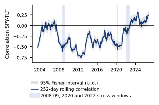
 MFM_ch6_spy_tlt_rolling

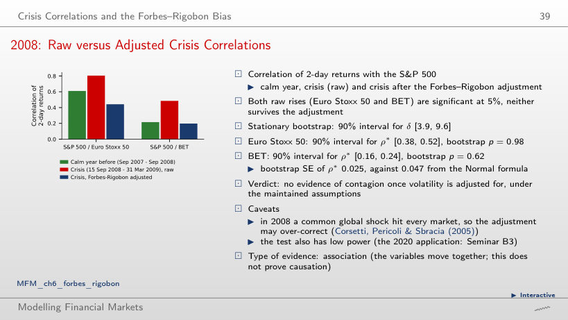
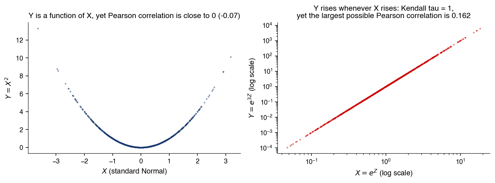
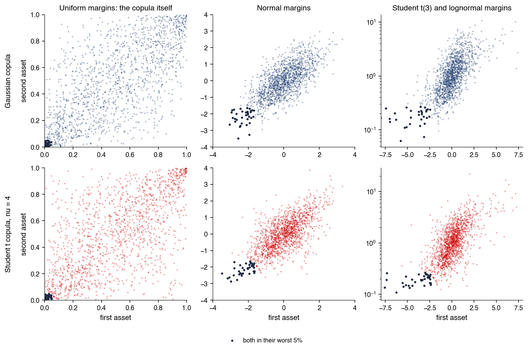
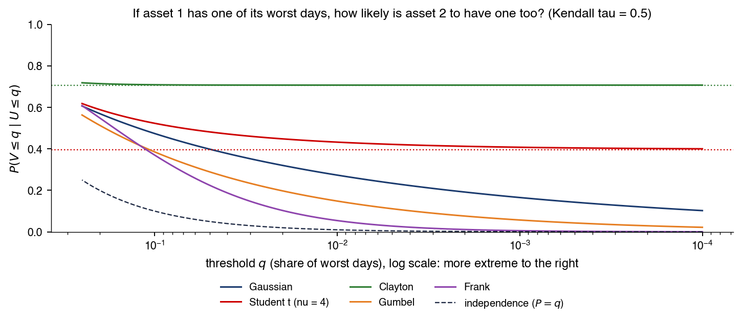
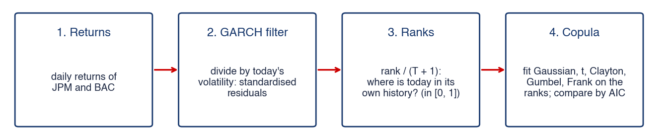
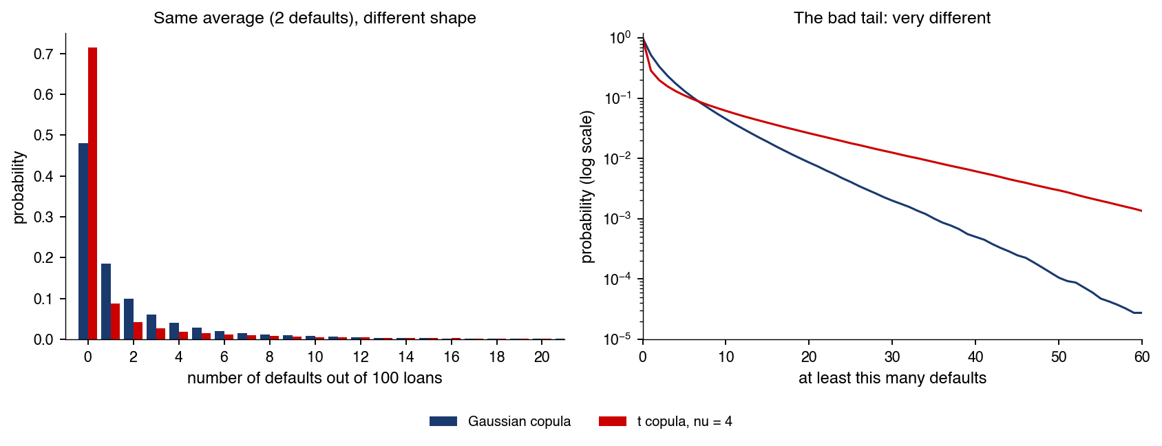

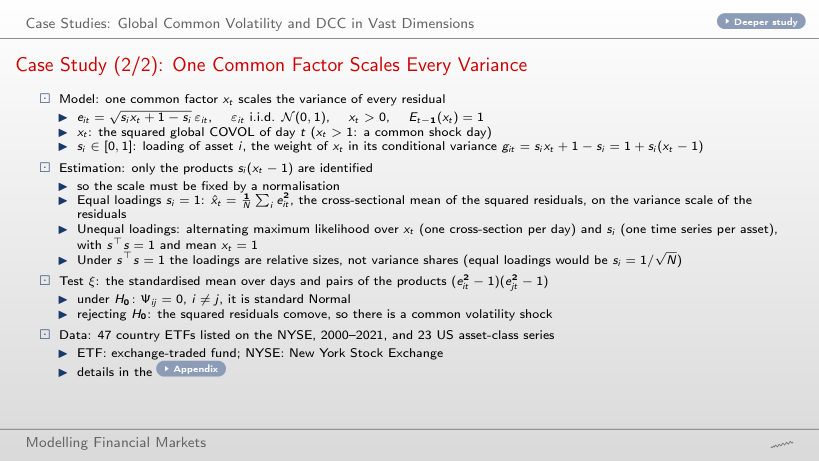
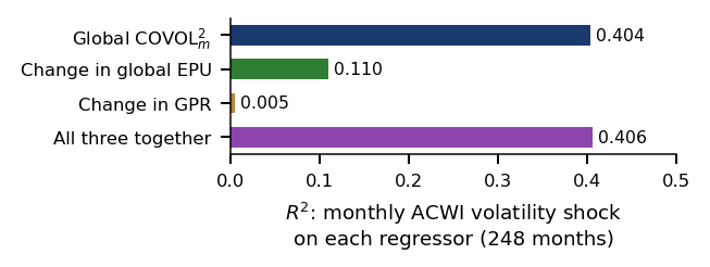
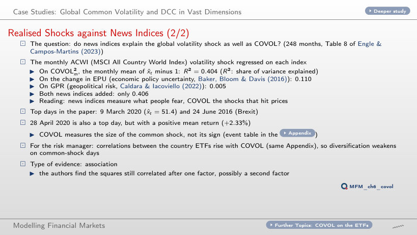
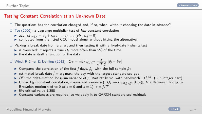
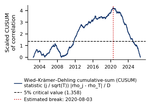
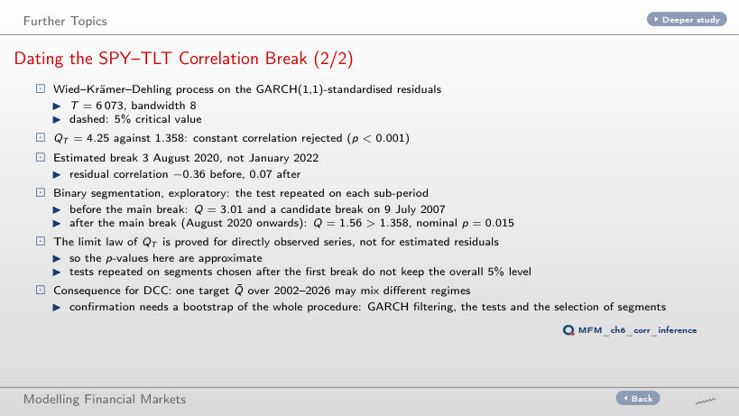
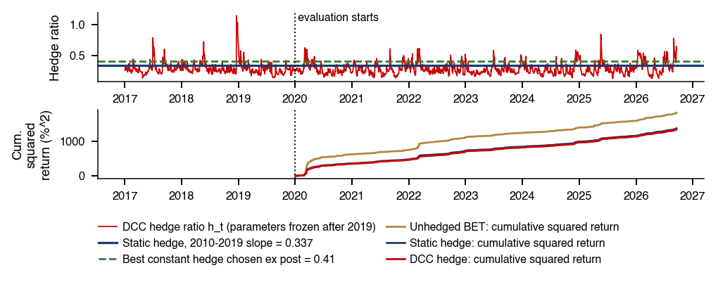
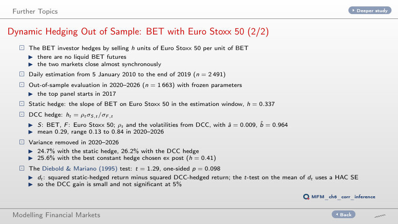
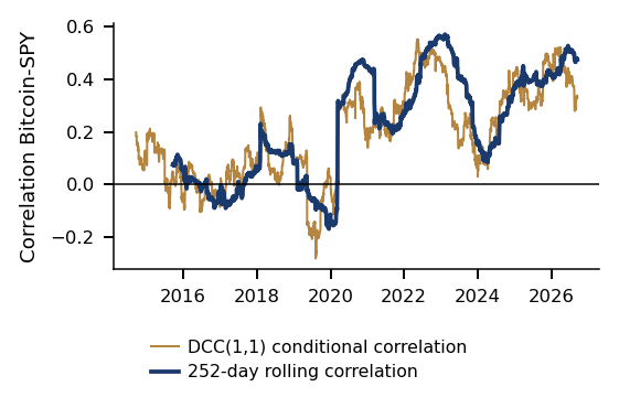
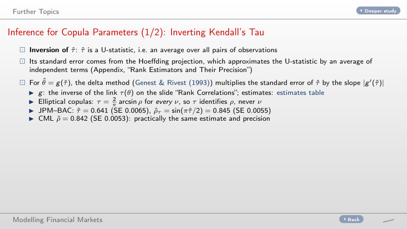
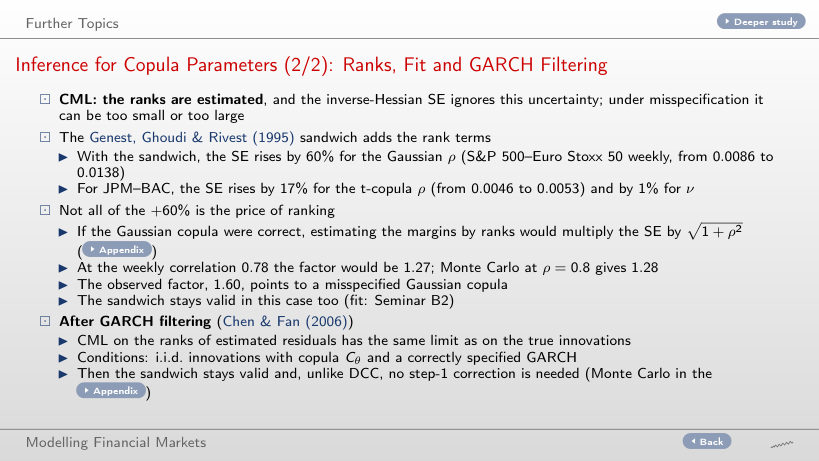
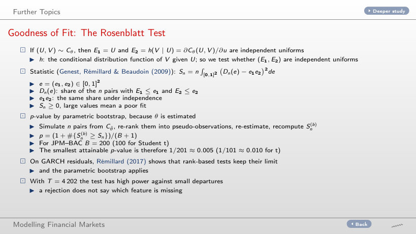
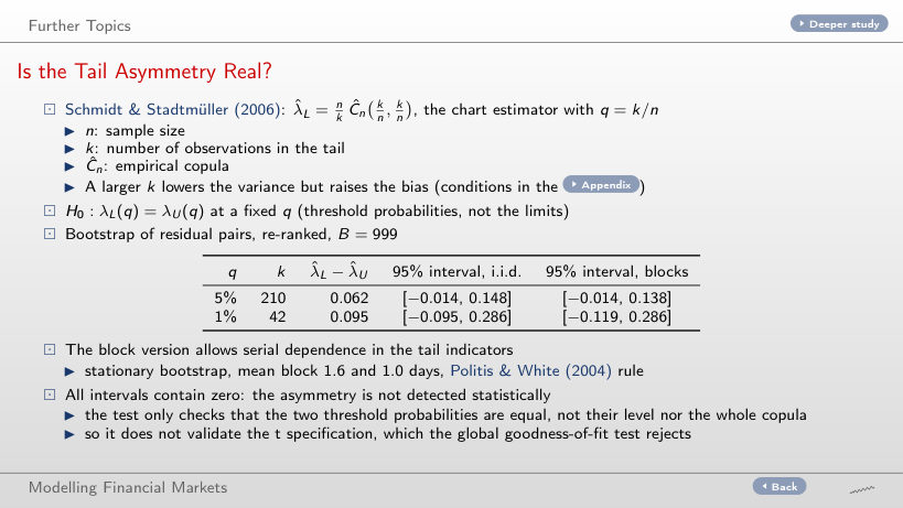
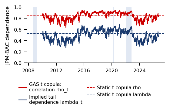
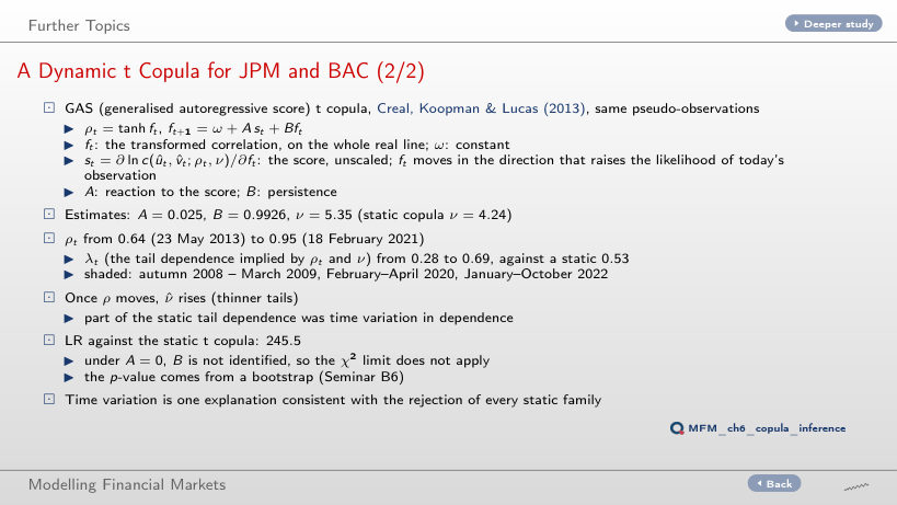
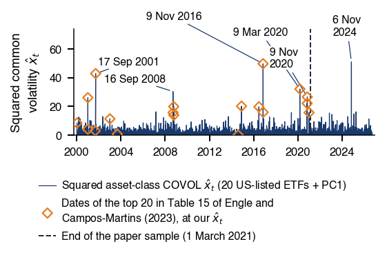

 Measuring Statistical Risk