Bucharest University of Economic Studies IDA Institute Digital Assets Blockchain Research Center AI4EFin Artificial Intelligence for Energy Finance Romanian Academy, Institute for Economic Forecasting MSCA Digital Finance
“We provide a framework for integration of high-frequency intraday data into the measurement, modeling, and forecasting of daily and lower frequency return volatilities and return distributions.” — Andersen, Bollerslev, Diebold & Labys (2003)
Realised variance (RV), the sum of squared 5-minute returns, measures each day's variance almost without a model
annualised volatility from the mean RV: 12.9% for SPY (the S&P 500 exchange-traded fund), 45.1% for Bitcoin
Overnight returns carry 38% of SPY's daily variance, although the market is closed for 17.5 hours
Jump tests on 1 489 SPY days: 236 rejections at 5% without correction
17 after the periodicity correction and false discovery rate (FDR) control
Out of sample, SPY 2022–2026: the log-HAR model (heterogeneous autoregressive) has a QLIKE (quasi-likelihood) loss of 0.310, against 0.343 for GARCH(1,1)-t
We provide a framework for integration of high-frequency intraday data into the measurement, modeling, and forecasting of daily and lower frequency return volatilities and return distributions.
Volatility drives risk, option prices and portfolio weights, but it is never observed. One daily return is a single draw from a distribution whose dispersion we want to estimate, and GARCH (Generalised AutoRegressive Conditional Heteroskedasticity) infers today's variance from past daily returns through a model. The chapter's question is how to measure a volatility we never see. The idea of Andersen & Bollerslev (1998) is that the sum of squared intraday returns measures the day's variance almost without a model; Andersen, Bollerslev, Diebold & Labys (2003) then use it to model and forecast volatility. Computed from 5-minute returns, the annualised volatility from the mean realised variance (RV) is 12.9% for SPY, the exchange-traded fund on the S&P 500 (Standard & Poor's), and 45.1% for Bitcoin. Overnight returns carry 38% of SPY's daily variance, although the market is closed for 17.5 hours.
Measurement has its own problems. Microstructure noise biases RV at very high frequencies; the SPY signature plot is approximately flat: 12.9% at 5 minutes, 12.8% at 30 minutes and 13.0% at 130 minutes. Jumps separate news from the continuous component, but daily tests need a correction for multiple testing. Of 1,489 daily tests on SPY, 236 reject at 5% without correction; after the periodicity correction and false discovery rate (FDR) control, 17 jump days remain.
Once measured daily, volatility can be modelled directly. The HAR (heterogeneous autoregressive) model of Corsi (2009) explains tomorrow's RV by its averages over one day, one week and one month. Out of sample, over 1,180 forecasts for SPY in 2022–2026, log-HAR has a QLIKE (quasi-likelihood) loss of 0.310 against 0.343 for GARCH(1,1)-t; the Diebold–Mariano test gives \(t = -2.30\) and \(p = 0.021\). MSE (Mean Squared Error) comparisons are inconclusive, because a few crisis days dominate the squared errors. The chapter ends with the question of whether volatility is rough, and how much of that roughness measurement error can produce.
Left: SPY realised volatility (including the overnight return) and the GARCH(1,1)-t and log-HAR forecasts, annualised, 2022–2026; right: the cumulative QLIKE loss of each model minus that of log-HAR (a rising curve means log-HAR is better). Interactive chart: “Forecasts over Time (1/2)” →
What you will be able to do
Compute daily realised variance, its standard error and a confidence interval from intraday prices.
Interpret a signature plot as a diagnosis of microstructure noise.
Compute the ratio jump test with false discovery rate control.
Compute the log-HAR estimates and interpret their persistence.
Derive the QLIKE loss from the Normal likelihood.
Interpret comparisons of variance forecasts: Diebold–Mariano, Mincer–Zarnowitz and the Model Confidence Set.
AppendixAsymptotic theory, noise- and jump-robust estimators and model extensions.
Motivation: Measuring Latent Volatility
Volatility is a parameter of the conditional distribution of returns, not an observable. Every model of the previous chapters inferred it indirectly: GARCH from the sequence of past daily returns, VaR (Value-at-Risk) models from that conditional variance. This chapter starts from the opposite end. Intraday prices contain hundreds of returns per day, and their squares add up to a measurement of the day's variance that needs almost no model. The section fixes what is measured, how this measurement differs from a forecast, and which intraday data the chapter uses.
Part I is measurement and diagnosis: the realised variance (RV) of a day, its precision, the bias that microstructure noise creates at high sampling frequencies, and the separation of jumps from continuous price moves.
Part II is modelling and forecasting: the stylised facts of realised volatility, the heterogeneous autoregressive (HAR) model and the out-of-sample comparison of HAR forecasts with those of generalised autoregressive conditional heteroskedasticity (GARCH) models from Chapter 5.
Three extensions follow the core path:
rough volatility;
a case study on machine learning against HAR, together with a second one on partial variances;
research assisted by artificial intelligence (AI).
Detailed examples are in Further Topics, and the asymptotic theory, the noise- and jump-robust estimators and the model extensions are in the Appendix.
In brief
What we will explain
Part I, measurement and diagnosis: realised variance and its precision, microstructure noise, jumps
Part II, modelling and forecasting: stylised facts, the HAR model, forecast evaluation against GARCH
Volatility enters risk measurement (Chapters 7 and 8), option pricing (Chapter 12) and portfolio weights (Chapter 4), yet it is never observed. A single daily return is one draw from a distribution whose dispersion we want to know. Its square is an unbiased but very noisy estimate of that dispersion, and a GARCH model therefore infers today's variance from a long history of daily returns, through a parametric recursion.
The alternative uses the information inside the day. Between the open and the close there are hundreds of price changes, and the sum of their squares measures the variance of that day almost without a model (Andersen & Bollerslev, 1998). The idea goes back to Merton (1980), who showed that the variance of returns, unlike the mean, is estimated more precisely when the same time span is sampled more often: the precision of a variance estimate grows with the number of observations, whereas the precision of a mean depends only on the length of the span.
Realised variance is an ex-post measurement of day \(t\), available after the close of that day.
The GARCH variance is a conditional forecast of day \(t\), made with the information available at the end of day \(t-1\).
The first answers "how variable was the day?", the second "how variable do we expect the day to be?". The forecast evaluation of this chapter uses the first to judge the second.
The two main assets have different trading clocks. SPY is an exchange-traded fund (ETF), a fund whose units trade on an exchange, that tracks the Standard & Poor's 500 stock index; it trades in the regular US (United States) session, from 09:30 to 16:00 New York time. Bitcoin trades continuously, and its daily intervals run from midnight to midnight in Coordinated Universal Time (UTC). The VIX, the Volatility Index of the Chicago Board Options Exchange, is an option-based measure of expected volatility and serves as a comparison for realised volatility in the section on stylised facts.
All series end on 18 September 2026. Returns are log returns in per cent, \(r_i = 100(\ln P_i - \ln P_{i-1})\), where \(P_i\) is the price at the end of bar \(i\). Times quoted in the chapter and on the charts mark the end of each 5-minute interval: the return labelled 09:35 is the first SPY return of the day, from 09:30 to 09:35. The full description of the samples is in Further Topics.
In brief
SPY: an Exchange-Traded Fund (ETF) tracking the Standard & Poor's 500 stock index
ETF: a fund whose units trade on an exchange
UTC means Coordinated Universal Time
Bitcoin daily intervals run midnight to midnight in that time zone
VIX: the Volatility Index of the Chicago Board Options Exchange (CBOE)
an option-price measure of expected volatility
All series end on 18 September 2026
Returns \(r_i = 100(\ln P_i - \ln P_{i-1})\) in %, \(P_i\): the price at the end of bar \(i\)
Charts and times quoted in this chapter mark the end of each 5-minute interval
Volatility is latent; realised variance measures it ex post from intraday returns, while GARCH forecasts it ex ante from daily returns. The next section defines realised variance, shows it on single days and on the daily series of SPY and Bitcoin, and gives its precision.
Realised Variance
This section defines the object of measurement, the integrated variance of a day, and its estimator, the realised variance. The framework is a continuous-time model of the log price with a time-varying spot volatility. Under this model, the sum of squared intraday returns converges to the integrated variance as the sampling interval shrinks, and a central limit theorem gives the precision of the measurement on a given day. The theory is then applied to SPY and Bitcoin: one extreme day, the daily series over 2020–2026 and the split of SPY's variance between the trading session and the night.
Day \(t\) is divided into \(M\) intervals of equal length \(\Delta = 1/M\), measured in days, with intraday returns \(r_{t,i}\),\(i = 1, \dots, M\). The return of the session is the sum \(r_t = \sum_i r_{t,i}\), because log returns add up over time. Variances are expressed in \(\%^2\) per day; annualised volatilities are \(\sqrt{252 \times \text{variance}}\) for SPY, which trades on 252 days a year, and \(\sqrt{365 \times \text{variance}}\) for Bitcoin, which trades every day. The SPY overnight return, from the previous close to the open, lies outside the 5-minute bars and is treated separately.
The log price follows the diffusion
\[dp(s) = \mu(s)\,ds + \sigma(s)\,dW(s),\]
(9.1)
where \(W\) is a standard Brownian motion (Chapter 11), \(\mu(s)\) the drift and \(\sigma(s)\) the spot volatility. In (9.1)\(\sigma(s)\) is itself a stochastic process: it changes within the day, for example between the open and midday, and from one day to the next.
In brief
Question: how do we turn a day's 5-minute returns into a measurement of that day's variance?
Notation: day \(t\) has \(M\) intervals of length \(\Delta = 1/M\), returns \(r_{t,i}\), daily return \(r_t = \sum_i r_{t,i}\)
the spot variance accumulated over the day. In this chapter IV always denotes integrated variance, never implied volatility. If \(\sigma\) is independent of \(W\) (no leverage effect) and the drift is zero, or determined by the path of \(\sigma\), then conditionally on the path of \(\sigma\) the daily return is Normal, \(r_t \mid \sigma \sim N(\int\mu, \mathrm{IV}_t)\). The daily return is thus a draw from a Normal distribution whose variance is the random quantity (9.2).
With leverage, that is, when shocks to \(\sigma\) are correlated with \(W\), this conditional normality fails. The limit theory of realised variance given below still holds, in the framework of Itô semimartingales, which is described in the Appendix.
In brief
Integrated variance of day \(t\): the quantity we want to measure
\(\IV_t = \displaystyle\int_{t-1}^{t} \sigma^2(s)\,ds\): the spot variance accumulated over the day
in this chapter IV always means integrated variance, never implied volatility
Given the path of \(\sigma\), the daily return is Normal: \(r_t \mid \sigma \sim N(\int\mu, \IV_t)\)
assumption: \(\sigma\) is independent of \(W\) (no leverage effect: price falls do not raise volatility)
assumption: the drift is zero (or fixed by the path of \(\sigma\))
With a leverage effect (Appendix: Itô semimartingales) this conditional normality fails, but the limit theory of realised variance (RV, next slide) still holds
The realised variance of day \(t\) is the sum of the squared intraday returns,
\[\mathrm{RV}_t = \sum_{i=1}^{M} r_{t,i}^2,\]
(9.3)
and the realised volatility is \(\sqrt{\mathrm{RV}_t}\). The squares are used because over a short interval \(\mathbb{E}[r_{t,i}^2 \mid \sigma] \approx \sigma^2(s_i)\,\Delta\), so their sum approximates the integral (9.2). The convergence is not that of a Riemann sum, however: the observed squared increments are random, and what their sum converges to is the quadratic variation of the log price.
The drift contributes terms of order \(\Delta\) per day, which vanish as \(M \to \infty\); for SPY the mean 5-minute return is below 1% of its standard deviation. No parameter is estimated in (9.3), so \(\mathrm{RV}_t\) is a model-free measurement of one day's variance.
The squared daily return \(r_t^2\) is the special case \(M = 1\). With zero drift it is unbiased for \(\mathrm{IV}_t\), but it is extremely noisy; the gain from intraday data is precision, not the removal of a bias.
In brief
Realised variance: the sum of squared intraday returns
Why squares: the conditional means of the squared increments approximate \(\int_{t-1}^{t} \sigma^2(s)\,ds\)
over a short interval \(\E[r_{t,i}^2 \mid \sigma] \approx \sigma^2(s_i)\,\Delta\)
the observed sum of squares converges to the quadratic variation; it is not a Riemann sum
Quadratic variation of day \(t\), with \(p = 100\ln P\): \([p]_t - [p]_{t-1} = \operatorname{plim}_{M \to \infty} \sum_{i=1}^{M} r_{t,i}^2 = \IV_t\) for a price without jumps Barndorff-Nielsen & Shephard (2002)
The drift adds terms of order \(\Delta\) per day, which vanish as \(M \to \infty\); for SPY the mean 5-minute return is below 1% of its standard deviation
No parameters to estimate: \(\RV_t\) is a model-free measurement of one day's variance
The squared daily return \(r_t^2\) is the special case \(M = 1\)
The interactive chart shows a single trading day of SPY on 5-minute bars. The left panel shows the price path and the right panel the running sum of squared returns, which reaches the day's RV at the close. The drop-down list selects the day; the default is 7 April 2025, the most volatile day of the sample.
Question for the room On 7 April 2025, RV is 45.1 %² and the largest absolute 5-minute return contributes 18.3 %². If only that return doubled, what would RV become?
Answer
About 100.0 %². That interval's contribution quadruples: 45.1 − 18.3 + 4 × 18.3 = 100.0 %². The value 63.4 %² doubles the variance contribution rather than the return; 180.4 %² assumes that all returns double. In the data, the +4.28% return of the interval ending at 10:15 contributes 41% of the day's RV.
SPY opened that day with an overnight log return of −3.27%, after tariff announcements. The 78 five-minute returns that followed give \(\mathrm{RV} = 45.1\%^2\), an annualised realised volatility of \(\sqrt{252 \times 45.1} = 107\%\). A single return of +4.28%, in the interval ending at 10:15, contributed 41% of the day's realised variance: the running sum jumps at that bar. From open to close the day ended +3.09%. The daily return hides the intraday swings that RV records.
The day shows the two sides of RV. On the one hand, it captures the intraday swings that a single open-to-close return of +3.09% conceals: the path went through large moves in both directions, and each of them adds its square to the sum. On the other hand, the measurement can be dominated by a few returns. When one interval brings 41% of the day's variance, the precision of RV on that day is lower than on a day with evenly spread returns, a point made formal by the confidence interval at the end of the section.
The overnight move of −3.27% is not part of the 78 intraday returns. For a measure of the total daily risk of SPY, the squared overnight return must be added, as shown two frames below.
In brief
Left: SPY on 5-minute bars on the most volatile day of the sample
Right: running sum of squared returns
SPY opened with an overnight log return of \(-3.27\%\), after tariff announcements
The interactive chart shows the daily realised volatility of SPY and Bitcoin, annualised and computed from 5-minute returns: for SPY over the regular US session, for Bitcoin over 24 hours. The gap in October 2025 is missing data. The slider removes the most volatile days from the mean, to show how sensitive the average level is to a few extreme observations.
Question for the room The SPY volatility computed from mean RV is 12.9% a year, and the daily median is 9.7%. How much does the first value fall if the 20 most volatile days are left out?
Answer
To 11.9%: 20 days, i.e. 1.3% of the 1,489, raise the volatility computed from mean RV by 1.0 percentage point. The mean of the variances is sensitive to a few extreme days; the median is not. For Bitcoin, leaving out its 20 most volatile days lowers the value from 45.1% to 41.6%.
For SPY the volatility computed from the mean RV, \(\sqrt{252\,\overline{\mathrm{RV}}}\), is 12.9% a year. The median day has 9.7%, and the range runs from 2.3% to 106.7%. For Bitcoin the corresponding value, \(\sqrt{365\,\overline{\mathrm{RV}}}\), is 45.1% a year, with a median of 37.8% and a maximum of 136.1% on 5 February 2026.
The volatility computed from the mean variance exceeds the median daily volatility for both assets. The reason is the right skewness of RV: a few very volatile days raise the mean of the variances, and therefore its square root, far above the typical day. The median is insensitive to these days; the mean is not.
Both series show volatility clustering: calm periods and turbulent periods alternate, and a volatile day is followed by other volatile days. This is the same regularity that GARCH models capture (Chapter 5). The difference is that every point on the chart is a measurement of one day, not the output of a fitted model. The persistence of these measurements is quantified in the section on stylised facts.
In brief
Annualised, from 5-minute returns
SPY: regular US (United States) session
Bitcoin: 24 hours
the gap in October 2025 is missing data
SPY: volatility from mean RV \(\sqrt{252\,\overline{\RV}} = 12.9\%\) p.a.
median day \(9.7\%\), range \(2.3\%\) to \(106.7\%\)
Volatility computed from mean variance exceeds the median: a few very volatile days raise the root-mean-square of daily volatilities
SPY trades for 6.5 hours, but its price also changes while the market is closed: the open differs from the previous close. The interactive chart splits the mean daily variance of SPY, annualised, into the intraday realised variance and the squared overnight return. The drop-down list chooses the aggregation (by year, quarter or month), and the slider sets a factor \(c\) by which the intraday RV is scaled up, one of the ways to account for the night without observing it.
Question for the room Volatility computed from mean intraday RV is 12.9% a year. If every intraday RV is multiplied by c = 1.62, approximately what does this volatility become?
Answer
About 16.4%: volatility is multiplied by √1.62, so 12.9% × √1.62 ≈ 16.4% (the readout shows 16.5% because it starts from the unrounded 12.93%). The value 20.9% applies the variance multiplier directly to volatility; 10.1% is the overnight component's volatility. Overnight returns bring 38% of the SPY daily variance; scaling matches mean variances, it does not reconstruct each day's overnight component.
Overnight returns carry 38% of SPY's daily variance, although the market is closed for 17.5 hours. The years 2020 and 2026 are partial. The scaling factor matches mean variances; it does not reconstruct the overnight component of each individual day.
The share of the night reflects how information arrives. Company earnings, macroeconomic data released before the open and the Asian and European sessions accumulate while the US market is closed, and they are priced at the open in a single jump of the price. The result is descriptive: it says where the variance falls, not why each overnight move occurs.
The annualised volatilities of the three returns are 16.6% close-to-close, 13.6% open-to-close and 10.1% overnight. For daily risk, the relevant measure is the total variance\(\mathrm{RV}_t + r_{\text{overnight},t}^2\), whose annualised mean corresponds to a volatility of 16.4%. The alternatives are to scale the intraday RV up by a constant or to combine the two parts with optimal weights (Hansen & Lunde, 2005). The arithmetic of adding day and night variances, and why \(13.6^2 + 10.1^2\) is not the right sum, is in Further Topics.
In brief
SPY, mean daily variance by year, annualised
intraday realised variance plus squared overnight return
2020 and 2026 are partial years
Overnight returns carry 38% of SPY's daily variance, although the market is closed for 17.5 hours
News (earnings, macro data, Asian and European sessions) accumulates and is priced at the open
Type of evidence: description (it shows what happened in the data, without testing a cause)
Annualised volatility
close-to-close \(16.6\%\)
open-to-close \(13.6\%\)
overnight \(10.1\%\)
For daily risk we use total variance: \(\RV_t + r_{\text{overnight},t}^2\)
annualised mean: \(16.4\%\), against \(12.9\%\) from intraday RV alone
Alternatives: scale intraday RV up, or weight the two parts optimally Hansen & Lunde (2005)
RV is a consistent estimator of \(\mathrm{IV}_t\) as \(M \to \infty\), but with \(M = 78\) it carries a sampling error. The feasible central limit theorem (CLT) of Barndorff-Nielsen & Shephard (2002) gives its size:
The variance of RV depends on the integrated quarticity \(\mathrm{IQ}_t = \int_{t-1}^{t}\sigma^4(s)\,ds\), which the realised quarticity \(\mathrm{RQ}_t\) estimates. From (9.5) the standard error is \(\mathrm{se}(\mathrm{RV}_t) = \sqrt{\tfrac{2}{3}\sum_i r_{t,i}^4}\). Fourth powers appear because the variance of a variance estimator depends on the fourth moment of the returns.
The 95% confidence interval (CI) is built on the log scale, \(\mathrm{RV}_t \exp(\pm 1.96\,\mathrm{se}(\mathrm{RV}_t)/\mathrm{RV}_t)\), so that it is always positive. With constant volatility within the day, \(\mathrm{se}/\mathrm{RV} \approx \sqrt{2/M}\), which is 16% for \(M = 78\): a single day's variance is measured with a relative error of about one sixth, much smaller than that of \(r_t^2\) but far from zero.
The limit in (9.5) is subtle. The asymptotic variance \(2\,\mathrm{IQ}_t\) is itself random, so the limit of \(\sqrt{M}(\mathrm{RV}_t - \mathrm{IV}_t)\) is a mixed Normal distribution. Replacing \(\mathrm{IQ}_t\) by its estimate \(\mathrm{RQ}_t\) is legitimate because the convergence is stable, that is, it holds jointly with every variable defined on the path; the formal statement is in the Appendix. The intervals for SPY and the days on which they widen are in Further Topics.
Realised variance (9.3) measures the integrated variance (9.2) of a day without parameters, and the CLT (9.5) gives its precision, about 16% relative error with 78 returns under constant intraday volatility. For SPY the mean RV corresponds to a volatility of 12.9% a year, and the night adds 38% of the daily variance. The next section asks why the sampling interval stops at 5 minutes rather than at every trade.
Microstructure Noise
The CLT of the previous section suggests sampling as often as possible, since the relative error falls like \(\sqrt{2/M}\). Observed prices, however, are not the efficient price of the model: they bounce between bid and ask, move on a discrete tick grid and stay stale between trades. This section models these effects as additive noise, derives the bias they induce in RV and the frequency that balances bias against sampling error, and checks on the course data whether 5-minute sampling is coarse enough.
If more returns shrink the relative error of RV, the natural question is why not use every trade. The answer is that the observed log price is not the efficient log price of (9.1). The standard model writes
where \(p^*_i\) is the efficient (true) log price, \(r^*_i\) the efficient return and \(\varepsilon_i\) the noise in the observed price. The sources of \(\varepsilon\) are the bid–ask bounce, the tick size, which makes prices discrete, and stale quotes; their economics is the subject of Chapter 10.
In brief
Question: why not use every trade?
more returns shrink the relative error of RV (\(\sqrt{2/M}\))
Observed prices are not the efficient price: \(p^{\text{obs}}_{i} = p^*_{i} + \varepsilon_{i}\)
so \(r_i = r^*_i + \varepsilon_i - \varepsilon_{i-1}\)
\(p^*_i\): the efficient (true) log price, \(\varepsilon_i\): the noise in the observed price, \(r^*_i\): the efficient return
Sources of \(\varepsilon\): bid–ask bounce, tick size (price discreteness), stale quotes (Chapter 10)
Following Zhang, Mykland & Aït-Sahalia (2005) and Hansen & Lunde (2006), suppose the noise is i.i.d. with variance \(\omega^2\), independent of the efficient price, and that a day has \(n\) returns. With zero drift and no leverage,
Each squared return carries \(\mathbb{E}[(\varepsilon_i - \varepsilon_{i-1})^2] = 2\omega^2\) of noise, so the bias in (9.7)grows linearly with the sampling frequency. Adjacent returns share the term \(\varepsilon_{i-1}\) with opposite signs, so the noise also induces a negative first-order autocorrelation, \(\mathrm{cov}(r_i, r_{i-1}) = -\omega^2\), a signature used below to detect it.
The mean squared error (MSE) of RV combines the two effects:
The first term is the discretisation error, which falls with \(n\); the second is the squared bias, which rises with \(n\). Minimising their sum gives the MSE-optimal number of returns \(n^*\) in (9.8)(Bandi & Russell, 2008); the derivation is in the Appendix.
A numerical example fixes the orders of magnitude. With \(\mathrm{IV} = 1\%^2\) and constant volatility within the day, \(\mathrm{IQ} = \mathrm{IV}^2 = 1\)(\(\%^4\)); with \(\omega = 0.01\%\),\(\omega^2 = 10^{-4}\%^2\). The bias \(2n\omega^2\) is then 0.016 at 5 minutes (\(n = 78\)) and 4.680 at one-second sampling, almost five times the variance being measured. The optimal number of returns is \(n^* = 292\), one return every 80 seconds.
\(\E[\RV^{(n)}_t \mid \sigma] = \IV_t + 2n\omega^2\) (zero drift, no leverage): each squared return carries \(2\omega^2\) of noise, so the bias grows with the sampling frequency
MSE (mean squared error) optimal number of returns \(n^* = \left(\text{IQ}/(4\omega^4)\right)^{1/3}\)Bandi & Russell (2008): more returns cut the first term, but raise the second; derivation in the Appendix
Numbers, with \(\IV = 1\%^2\) and \(\omega = 0.01\%\), so \(\omega^2 = 10^{-4}\%^2\)
constant volatility within the day, so \(\text{IQ} = \IV^2 = 1\) (%\(^4\))
the bias \(2n\omega^2\) is \(0.016\) (%\(^2\)) at 5 minutes (\(n = 78\)) and \(4.680\) at 1 second, larger than IV itself
Optimal number of returns: \(n^* = 292\) (one return every \(80\) s)
Formula (9.8) cannot be applied directly: \(\omega^2\) and \(\mathrm{IQ}_t\) are unknown and differ across assets and days. The optimal frequency also falls quickly as the noise grows. With \(\omega = 0.01\%\),\(n^* = 292\); with \(\omega = 0.1\%\),\(n^* = 14\), about one return every 29 minutes.
The practical answer is sparse sampling at 5 minutes, \(n = 78\) in a 6.5-hour session. At this frequency the bias \(2n\omega^2\) stays small for liquid assets, and the relative discretisation error is \(\sqrt{2/78} = 16\%\). The cost is that most trades are discarded. Liu, Patton & Sheppard (2015) compare almost 400 estimators on 31 assets and find that 5-minute RV is rarely beaten. The course data are 5-minute bars, the finest grid available, so the question becomes whether 5 minutes is sparse enough for SPY and Bitcoin; the signature plot answers it.
In brief
Question: which frequency, when \(n^*\) depends on \(\omega^2\) and \(\text{IQ}_t\)?
both are unknown and different across assets
The optimal frequency falls fast as the noise grows
\(n^* = 292\) with \(\omega = 0.01\%\)
\(n^* = 14\) (one return about every 29 minutes) with \(\omega = 0.1\%\)
A signature plot shows the volatility implied by the mean RV against the sampling interval. If noise of the type (9.6) matters, the curve rises as the interval shrinks, because the bias in (9.7) grows with \(n\). The interactive chart shows the annualised volatility from mean RV for SPY and Bitcoin, computed on one grid and as the average over all shifted grids. The drop-down list selects the period, and the slider adds artificial i.i.d. noise of standard deviation \(\omega\) to the log prices, to show how the curve would look with noise.
Question for the room Using the approximation of 78 intervals per day, what standard deviation ω of independent noise added to log prices raises SPY's 5-minute volatility from 12.9% to approximately 14.0% a year?
Answer
About ω = 0.027%. Solving 252 × (mean RV + 2 × 78 × ω²) = 14² gives ω ≈ 0.02708%; on the slider, 0.027% gives 13.99% and 0.028% gives 14.07%. The value 0.019% incorrectly uses 4nω²; 0.038% uses nω². The actual signature plot stays approximately flat, between 12.6% and 13.1%: compatible with a much smaller noise bias at 5 minutes, without ruling out noise.
The curve is approximately flat in the sampling interval. For SPY the annualised volatility is 12.9% at 5 minutes, 12.8% at 30 minutes and 13.0% at 130 minutes; for Bitcoin, 45.1% at 5 minutes and 44.5% at 6 hours. The first-order autocorrelation of 5-minute returns is −0.008 for SPY and 0.005 for Bitcoin. Neither diagnostic shows noise at 5 minutes. A flat curve is compatible with a small noise bias; it does not prove the absence of noise.
The diagnosis has a built-in limit. Bars of 5 minutes can only diagnose sampling at 5 minutes and coarser; they say nothing about the noise at higher frequencies, where tick data would be needed. The result supports a description: on these assets and this sample, 5-minute RV shows no visible noise bias.
Noise-robust estimators computed on the same 5-minute SPY data illustrate the point. Their ratios to RV are 0.84 for two-scale RV on the standard grids and 0.97 when the day's first and last prices are added to every grid; 0.92 for the realised kernel with jittered end points and 0.95 with the raw end prices. These differences come from the estimators, not from a measured noise bias: with 78 bars, the theoretical versions drop part of the first and last intervals of the day, which are the most volatile. Both estimators are described in Further Topics.
The result agrees with Liu, Patton & Sheppard (2015). Noise-robust estimators pay off when the noise is large relative to the signal, as with tick or second-level data and illiquid assets; for liquid assets sampled at 5 minutes, plain RV is hard to beat.
In brief
Annualised volatility from mean RV by sampling interval
one grid vs the average over all shifted grids (subsampling)
Approximately flat in the sampling interval: compatible with a small noise bias, not proof of no noise
SPY \(12.9\%\) at 5 minutes, \(12.8\%\) at 30, \(13.0\%\) at 130
Bitcoin \(45.1\%\) at 5 minutes, \(44.5\%\) at 6 hours
First-order autocorrelation of 5-minute returns: \(-0.008\) (SPY), \(0.005\) (Bitcoin): i.i.d. noise would make it negative (\(-\omega^2\)), so no visible noise at 5 minutes
Limit of this dataset: 5-minute bars say nothing about noise below 5 minutes
Noise-robust estimators (Further Topics), as ratios to RV on SPY: differences between estimators, not a measured noise bias
two-scale RV on the standard grids: \(0.84\); with the day's first and last price in every grid: \(0.97\)
realised kernel with jittered end points: \(0.92\); with the raw end prices: \(0.95\)
with 78 bars, the theoretical versions drop part of the first and last intervals of the day, the most volatile ones
Microstructure noise makes RV a biased estimator at high frequencies, with bias \(2n\omega^2\)(9.7), and the MSE trade-off (9.8) gives an optimal frequency that falls fast with the noise. On SPY and Bitcoin the signature plot is approximately flat from 5 minutes up, so 5-minute RV is the measurement used in the rest of the chapter. The next section drops the assumption that the price path is continuous.
Jumps
The diffusion (9.1) has continuous paths, but prices also jump on news. With jumps, RV converges to the integrated variance plus the sum of squared jumps, and the two components have different economic content: jumps are less persistent than diffusive volatility and are priced differently in options. This section introduces bipower variation, which estimates the continuous part, the ratio test for a jump on a given day, and the control of false discoveries when the test is repeated on every day of the sample.
The question is how much of a day's variance comes from jumps and how jumps can be separated from diffusion. Adding a jump process \(J\) to the model gives \(dp = \mu\,ds + \sigma\,dW + dJ\) (Chapter 11). The quadratic variation then has two parts,
where \(\kappa_j\) are the sizes of the jumps that occur on day \(t\).
The separation matters for two reasons:
Jumps are less persistent than the diffusive component of volatility, so a forecasting model that treats them alike overstates the persistence after a jump day.
Jumps price differently from diffusive risk in options (Chapter 12).
with \(Z \sim N(0,1)\), so that \(\mu_1 = 0.798\) and \(\mu_1^{-2} = \pi/2 = 1.571\); the factor \(M/(M-1)\) is a finite-sample normalisation. The base case for (9.10) is jumps of finite activity and no noise; other settings need extra conditions.
The mechanism is simple. A jump of finite activity enters a single return. In RV that return is squared, so the jump contributes \(\kappa^2\). In BV (Bipower Variation) it is multiplied by a neighbouring return of diffusive size, of order \(\sqrt{\Delta}\), so its effect vanishes as \(M\) grows. The jump part of the day is estimated by \(\max(\mathrm{RV}_t - \mathrm{BV}_t, 0)\).
A four-return example shows the arithmetic. With returns \(0.1, 0.1, 0.1, 1.0\) (%), \(\mathrm{RV} = 1.03\) and \(\mathrm{BV} = \frac{\pi}{2}\cdot\frac{4}{3}(0.01 + 0.01 + 0.10) = 0.25\), so the jump part is \(0.78\)(\(\%^2\)): the last return contributes almost all of RV but little to BV.
The numerator of (9.11) is the relative jump share of the day, and the denominator its standard error under the null of no jumps. The constant \(\theta\) is the asymptotic variance constant, and the tripower quarticity
\[\mathrm{TQ}_t = M \mu_{4/3}^{-3}\frac{M}{M-2}\sum_i |r_{t,i}|^{4/3}|r_{t,i-1}|^{4/3}|r_{t,i-2}|^{4/3},\]
with \(\mu_{4/3} = \mathbb{E}|Z|^{4/3}\), estimates the integrated quarticity robustly to jumps.
Under the null of no jumps \(z_t \to N(0,1)\). A jump makes \(\mathrm{RV}_t > \mathrm{BV}_t\) and \(z_t\) large and positive, so the test is one-sided. The jump days plotted on the next frame use the level \(\alpha = 0.1\%\), with critical value 3.09. On a significant day the jump part is \(J_t = \mathrm{RV}_t - \mathrm{BV}_t\) and the continuous part \(C_t = \mathrm{RV}_t - J_t\); on the other days \(J_t = 0\).
The interactive chart marks the days with a significant jump on the series of daily RV. Red points are the jump days, with point size proportional to the jump part \(J_t\). The slider sets the test level \(\alpha\), and the drop-down list chooses between no correction for multiple testing and the Benjamini–Hochberg rule, explained two frames below.
Question for the room If none of the 1,489 SPY days contains jumps and each test rejects incorrectly with probability 5%, how many false rejections do we expect before adjusting for multiple testing?
Answer
About 74: the expected count is 1,489 × 0.05 = 74.45, not a guaranteed sample count; independence across days is unnecessary for this expectation. In the data, the test without the intraday-periodicity adjustment gives 236 rejections at 5%, and Benjamini–Hochberg (FDR at 5%) retains 43. After the periodicity adjustment, Benjamini–Hochberg retains 17.
At the 0.1% level, SPY has 36 jump days of 1,489 (2.4%), and jumps make up 2.8% of total realised variance. On a jump day, the jump is on average 36% of that day's RV. The largest statistic, \(z = 5.2\), falls on 27 August 2021 in the interval 10:00–10:05, during the Jackson Hole speech of the chair of the Federal Reserve. Bitcoin has 67 jump days of 659 (10.2%), but jumps make up only 1.8% of its variance.
The two markets differ in the type of jumps. Bitcoin has many small jumps on quiet days, often at weekends, where one isolated move dominates an otherwise calm day; the relative jump share in (9.11) is then high although the jump itself is small. This is why Bitcoin has more than four times the share of jump days of SPY but a smaller share of variance from jumps.
The turbulent days of April 2025 are mostly not jump days. On those days many large returns occur in a row, so BV rises together with RV and the ratio stays small. The test detects isolated discontinuities, not volatile days: a day of sustained turbulence is classified as diffusive.
In brief
Red points: days with a significant jump at the 0.1% level
point size proportional to the jump part \(J_t\)
SPY: 36 jump days of 1 489 (2.4%)
jumps are 2.8% of total realised variance
on a jump day the jump is on average 36% of that day's RV
largest statistic: 2021-08-27 (\(z = 5.2\)), 10:00–10:05: the Jackson Hole speech of the Fed chair
Bitcoin: 67 jump days of 659 (10.2%), but only 1.8% of variance
many small jumps on quiet days (weekends), where one isolated move dominates the day
The turbulent days of April 2025 are mostly not jump days
Applied to 1,489 days at the 5% level, the test rejects on 236 days. If no day contained a jump, about 74 false rejections would be expected. The question is which of the 236 rejections are false. Part of the excess comes from intraday seasonality (Further Topics): volatility is higher at the open and the close, which biases BV downwards and makes the test over-reject. Dividing the returns by the periodicity factor \(f_i\) of Boudt, Croux & Laurent (2011) already cuts the 5% rejections from 236 to 169.
The remaining problem is multiplicity. Benjamini & Hochberg (1995) control the false discovery rate (FDR), the expected share of false rejections among all rejections. The \(N\)\(p\)-values are sorted, \(p_{(1)} \le \dots \le p_{(N)}\), and the \(k\) smallest are rejected, where
\[k = \max\{\,j : p_{(j)} \le j\,q/N\,\},\]
(9.12)
and \(q\) is the target FDR. Here each day's \(p\)-value is the one-sided \(1 - \Phi(z_t)\) of the ratio statistic. The rule (9.12) keeps \(\mathbb{E}[\text{false}/\text{rejections}] \le q\), with the ratio set to zero when nothing is rejected.
The guarantee requires valid \(p\)-values that are independent or positively regression dependent on the subset of true nulls (PRDS) (Benjamini & Yekutieli, 2001). Daily jump tests satisfy this only approximately. A worked example with five tests is in Further Topics.
In brief
1 489 daily tests at 5%: 236 rejections; which of them are false?
against 74 expected under no jumps
Part of the excess is intraday seasonality, higher volatility at the open and close (Further Topics)
dividing returns by the periodicity factor \(f_i\)Boudt, Croux & Laurent (2011) already cuts the days rejected at 5% from 236 to 169
\(k\): the largest index with \(p_{(k)} \le k q/N\); \(p_{(k)}\): \(k\)-th smallest \(p\)-value, \(N\): number of tests, \(q\): target FDR
here each day's \(p\)-value is the one-sided \(1 - \Phi(z_t)\) of the ratio statistic
the FDR, \(\E[\text{false}/\text{rejections}]\), stays \(\le q\) (false/rejections \(:= 0\) when nothing is rejected)
The guarantee needs valid \(p\)-values that are independent or positively regression dependent on the subset of true nulls (PRDS) Benjamini & Yekutieli (2001)
The number of SPY jump days depends strongly on the error rate controlled. On 1,489 days, the FDR at 5% retains 43 jump days and the FDR at 1% retains 14. The Bonferroni correction, which controls the family-wise error rate (FWER), the probability of at least one false rejection, at 5%, retains 7. With the periodicity correction followed by FDR control at 5%, 17 days remain. The fall from 236 unadjusted rejections to 17 does not identify which rejections were false; it states how many can be kept at a controlled error rate.
The result is descriptive, but it agrees with the literature. Bajgrowicz, Scaillet & Treccani (2016), on their sample and tests, find that without multiplicity control most detected jumps are spurious, and that the true ones are rare and cluster on news. Christensen, Oomen & Podolskij (2014), on tick data, find that most 5-minute "jumps" are steep but continuous bursts of volatility when observed at tick frequency.
A daily test answers whether day \(t\) contained a jump. Locating the jump within the day needs an intraday test, such as that of Lee and Mykland in the Appendix.
In brief
SPY, 1 489 days
without the periodicity correction, FDR at 5%: 43 jump days; at 1%: 14
Bonferroni (each day tested at \(5\%/1\,489\); family-wise error rate, FWER, 5%): 7
FDR 5% after the periodicity correction: 17
from 236 unadjusted rejections to 17: the drop does not identify which rejections were false
The standard error of RV uses fourth powers because the variance of RV is \(2\,\mathrm{IQ}_t/M\), and the integrated quarticity is estimated by \(\mathrm{RQ}_t\) in (9.5).
Intraday RV alone understates SPY's daily risk because overnight returns bring 38% of its daily variance.
Sampling every tick overstates variance because each squared return adds \(2\omega^2\) of noise, so the bias \(2n\omega^2\) in (9.7) grows with the number of returns.
In brief
Why does the standard error of RV use fourth powers of returns?
The variance of RV depends on integrated quarticity \(\text{IQ}_t\), estimated by \(\text{RQ}_t = \frac{M}{3}\sum_i r_{t,i}^4\)
Why is SPY's daily risk understated if you use intraday RV alone?
Overnight returns bring 38% of SPY daily variance
Why does sampling every tick overstate variance?
Every squared return adds \(2\omega^2\) of noise, so the bias \(2n\omega^2\) grows with the number of returns
Check Yourself: Measurement, Noise and Jumps (2/2)
A flat signature plot is compatible with a small noise bias at 5 minutes and coarser, but it does not rule out noise, and it says nothing about noise below 5 minutes. Bipower variation stays close to IV on a jump day because, with finite-activity jumps and no noise, the jump enters one return, which is squared in RV but multiplied by a small neighbour in BV. With 1,489 daily tests, \(p < 0.05\) on a given day is not evidence of a jump: jump-free days would produce about 74 false rejections at that level. The FDR controls the expected share of false rejections among the rejections, not the probability of any false rejection.
In brief
What does a flat signature plot tell you?
It is compatible with a small noise bias at 5 minutes and coarser; it does not rule out noise
What does it not tell you?
It says nothing about noise below 5 minutes
Why does bipower variation stay close to IV on a jump day while RV does not?
With finite-activity jumps and no noise, the jump enters a single return: squared in RV, multiplied by a small neighbour in BV
With 1 489 daily jump tests, why is “\(p < 0.05\)” not evidence of a jump?
At 5%, 1 489 jump-free days would give about 74 false rejections
What does the FDR control?
The FDR controls the expected share of false rejections among rejections
Section summary
Bipower variation (9.10) estimates the continuous part of the quadratic variation (9.9), and the ratio statistic (9.11) tests for a jump on a given day. Repeated over 1,489 days, the test needs both the periodicity correction and FDR control (9.12): for SPY the count falls from 236 rejections to 17 jump days. The next section turns from measurement to the regularities of the measured series.
Stylised Facts of Realised Volatility
With a daily measurement of volatility in hand, its properties can be studied as those of an observed time series. This section documents four regularities that a forecasting model must reproduce: the approximately lognormal distribution of RV, the near-normality of returns standardised by realised volatility, the slow decay of the autocorrelation of log RV, and the systematic gap between implied and realised volatility.
The interactive chart has two panels. The left panel shows the histogram of daily log RV of SPY with the density of the Normal distribution fitted to it. The right panel shows open-to-close returns scaled by their unconditional standard deviation (filled bars) and by \(\sqrt{\mathrm{RV}_t}\) (outline). The drop-down list selects the asset, and the slider moves the Box–Cox parameter \(\lambda\) from 0, the logarithm, to 1, the level of RV.
Question for the room For SPY, the skewness of log RV is 0.29 at λ = 0. Approximately what does it become when the Box–Cox parameter is moved to λ = 1?
Answer
About 20.0. At λ = 1, the transformation is RV − 1, which preserves RV's skewness (kurtosis 550). The value 3.9 corresponds to λ = 0.5 (the square root); 0.29 corresponds to the logarithm. Log RV's moments being close to those of the Normal distribution (0 and 3) does not establish conditional normality.
The skewness and kurtosis of the Normal distribution are 0 and 3. For SPY, RV has skewness 20.0 and kurtosis 550, whereas log RV has skewness 0.29 and kurtosis 3.21. For Bitcoin, log RV has skewness −0.27 and kurtosis 3.33. Open-to-close SPY returns have kurtosis 15.73, and 2.66 after division by \(\sqrt{\mathrm{RV}_t}\), with a standard deviation of 1.05; for Bitcoin the kurtosis falls from 7.56 to 2.77.
Volatility should be modelled in logs: the distribution of \(\ln \mathrm{RV}\) is close to Normal in both markets, whereas RV in levels is extremely skewed and heavy-tailed. The moments of log RV close to 0 and 3 do not establish that the conditional distribution is Normal, but they make linear models with Normal errors a reasonable approximation.
The heavy tails of daily returns (Chapter 1) come mostly, ex post, from changing volatility. Dividing each return by that day's realised volatility removes most of the excess kurtosis. Returns are then approximately a mixture of Normal distributions with variances \(\mathrm{IV}_t\), as the model of the Realised Variance section implies; the mixture is exact only without leverage and jumps.
A caveat applies to the kurtosis figures. The sample kurtosis can always be computed, but if the population fourth moment is infinite it estimates no finite population quantity (Chapter 1). The fall from 15.73 to 2.66 is a description of this sample, not an estimate of a population kurtosis.
In brief
Left: daily log RV of SPY and the Normal density
Right: open-to-close returns scaled
by their standard deviation (filled)
by \(\sqrt{\RV_t}\) (outline)
SPY skewness and kurtosis (the Normal distribution: 0 and 3)
RV: skewness \(20.0\), kurtosis \(550\)
log RV: skewness \(0.29\), kurtosis \(3.21\)
Bitcoin log RV: skewness \(-0.27\), kurtosis \(3.33\): model volatility in logs
Open-to-close returns: kurtosis \(15.73\), and \(2.66\) after dividing by \(\sqrt{\RV_t}\)
the sample kurtosis can be computed even when the population fourth moment is infinite; it then estimates no finite population kurtosis (Chapter 1)
standard deviation after dividing: \(1.05\)
Bitcoin: from \(7.56\) to \(2.77\)
Heavy tails of daily returns (Chapter 1) come mostly, ex post, from changing volatility
approximately a mixture of Normal distributions with variances \(\IV_t\)
exact only without leverage and jumps (section Realised Variance)
The interactive chart shows the sample autocorrelation function (ACF) up to 100 days for the log RV of SPY, computed on total variance, for the log RV of Bitcoin, and for squared daily SPY returns. The drop-down list adds a comparison: an autoregressive model of order one, AR(1), with a coefficient \(\rho\) chosen with the slider, or the ACF implied by the log-HAR model fitted to SPY in the next section.
Question for the room The autocorrelation of log RV for SPY is 0.64 at lag 1. What would it be at lag 22 for an AR(1) with the same lag-1 autocorrelation?
Answer
For an AR(1), lag-k autocorrelation is ρᵏ: 0.64²² ≈ 0.000054. The value 0.24 is the empirical lag-22 autocorrelation, not the AR(1) implication; dividing by 22 uses the wrong rule. The fitted log-HAR, seen as an AR(22), gives 0.63 at lag 1 and 0.24 at lag 22, as the data do, but understates lag-100 autocorrelation: about 0.02 against 0.10.
The log RV of SPY is highly persistent: its autocorrelation is 0.64 at lag 1, 0.24 at one month and still 0.10 at 100 days. An AR(1) with the same first-order autocorrelation would decay geometrically, to \(0.64^{22} \approx 0.00005\) at one month. The fitted log-HAR, read as an AR(22), gives 0.63 at lag 1 and 0.24 at lag 22, as the data do, but about 0.02 at lag 100 against 0.10 in the data.
In brief
Autocorrelations up to 100 days
log RV of SPY (total variance) and Bitcoin
squared daily SPY returns
SPY log RV: highly persistent dependence
\(0.64\) at lag 1, \(0.24\) at one month, still \(0.10\) at 100 days
an autoregressive AR(1) model would decay geometrically: \(0.64^{22} \approx 0.00005\)
a sample autocorrelation function (ACF) is consistent with long memory (autocorrelations decaying more slowly than geometrically) but cannot prove it
A sample ACF that decays this slowly is consistent with long memory, but cannot prove it: a sum of a few short-memory components with different persistence produces the same picture over finite horizons. The HAR model of the next section exploits exactly this observation.
Squared daily returns show the same persistence, hidden by noise: their first-order autocorrelation is only 0.20, because each \(r_t^2\) is a noisy measurement of the day's variance. The autocorrelation of \(r_t^2\) also requires a finite fourth moment, which Chapter 1 questions. RV removes most of the measurement noise and reveals the persistence of the underlying volatility.
Bitcoin's ACF has peaks at lags 7, 14, 21 and so on: a weekly cycle. Weekend RV is only 0.41 of weekday RV; on Saturday the annualised volatility is 27%, against 48% on Wednesday. At weekends there are no equity or macroeconomic releases and fewer institutional traders.
In brief
Squared daily returns show the same persistence, hidden by noise
autocorrelation at lag 1: \(0.20\)
the autocorrelation of \(r_t^2\) requires a finite fourth moment, which Chapter 1 questions
Bitcoin: peaks at 7, 14, 21, … days: a weekly cycle
weekend RV is only \(0.41\) of weekday RV (Saturday \(27\%\) vs Wednesday \(48\%\) p.a.)
no equity or macro news, fewer institutional traders
The VIX is the market's option-implied expectation of S&P 500 volatility over the next 30 calendar days. The interactive chart compares it with the realised volatility of SPY over the following trading days. The left panel shows the two series, and the right panel the gap between them. The slider sets the horizon of the realised volatility in trading days, and the second slider a date marked on both panels.
Question for the room The VIX exceeds the realised volatility over the next 21 trading days on 88% of days. Is that percentage alone sufficient to establish that the mean difference is positive?
Answer
No. A few large negative differences can outweigh many small positive ones. In this sample of 1,468 days, the mean difference is indeed positive, 4.36 percentage points (19.52% against 15.15%), but this follows from the sizes of the differences, not just from their signs. It is an ex-post volatility gap.
With a horizon of 21 trading days, the VIX has a mean of 19.52%, against 15.15% for the realised volatility that followed. The VIX was higher on 88% of the 1,468 days, by 4.36 percentage points on average. This mean ex-post gap is the starting point for the variance risk premium.
The gap has an economic interpretation, the variance risk premium (VRP) studied by Carr & Wu (2009) and by Bollerslev, Tauchen & Zhou (2009). Let \(Q_t = \tfrac{252}{21}\sum_{j=1}^{21} V_{t+j}\) be the annualised total variance over the next 21 trading days. The premium is the difference between its expectation under the risk-neutral measure \(\mathbb{Q}\) and under the physical measure \(\mathbb{P}\),
so the ex-post gap adds a forecast error to the premium. The sign of the realised gap on a given day does not identify the sign of the ex-ante premium, and the 88% figure alone does not even establish that the mean gap is positive; the size of the gaps does. The result supports a description of the sample. The regression of realised variance on \(\mathrm{VIX}^2\) is in Further Topics.
In brief
Left: VIX and SPY realised volatility over the next 21 trading days
Right: the gap between them
VIX mean \(19.52\%\) vs \(15.15\%\) realised afterwards
VIX was higher on 88% of 1 468 days, by 4.36 percentage points on average: the mean ex-post volatility gap
\(Q_{t} = \tfrac{252}{21}\sum_{j=1}^{21} V_{t+j}\): annualised total variance over the next 21 trading days
\(\text{VRP}_t = \E^{\mathbb{Q}}_t[Q_t] - \E^{\mathbb{P}}_t[Q_t]\): risk-neutral expectation (\(\mathbb{Q}\), from option prices) minus the real-world one (\(\mathbb{P}\)); VIX\(^2\) approximates the first term (Chapter 12)
VIX\(_t^2 - Q_t \approx \text{VRP}_t + (\E^{\mathbb{P}}_t[Q_t] - Q_t)\): the ex-post gap adds a forecast error to the premium
the sign of the realised gap does not identify the sign of the ex-ante premium
The stylised facts of realised volatility are four:
Log RV is close to Normal.
Returns standardised by realised volatility are close to Normal.
Log RV is highly persistent, with autocorrelation 0.10 at 100 days for SPY.
The VIX exceeds subsequent realised volatility on most days.
The first three facts motivate a linear model for \(\ln \mathrm{RV}\) with slowly decaying dependence, which the next section builds.
The HAR-RV Model
Since RV is observed daily, its dynamics can be modelled by regression rather than by a latent-variance recursion. The difficulty is the slow decay of the autocorrelation: a low-order autoregression decays too fast, and an unrestricted long autoregression has too many parameters. The heterogeneous autoregressive (HAR) model of Corsi (2009) resolves the tension with three regressors, RV averaged over a day, a week and a month. This section defines HAR and its log version, estimates both on SPY and Bitcoin, and introduces two extensions, HARQ and SHAR, which address the measurement error of RV and the sign of the returns.
The question is how to forecast tomorrow's RV when the autocorrelation of \(\ln \mathrm{RV}\) is still 0.10 at 100 days. Corsi (2009) proposes the regression
with \(\mathrm{RV}^{(w)}_t = \frac{1}{5}\sum_{j=0}^{4}\mathrm{RV}_{t-j}\) the average over the last week and \(\mathrm{RV}^{(m)}_t = \frac{1}{22}\sum_{j=0}^{21}\mathrm{RV}_{t-j}\) the average over the last month. The coefficients \(\beta_d\),\(\beta_w\) and \(\beta_m\) weight yesterday's RV and the weekly and monthly averages, \(\beta_0\) is a constant and \(\varepsilon_{t+1}\) the forecast error. Bitcoin trades every day, so its weekly and monthly averages use 7 and 30 days.
The motivation is the heterogeneous market hypothesis of Müller et al. (1997): traders operate at different horizons, daily, weekly and monthly, and each group reacts to volatility over its own horizon. This is the "H" of HAR, and HAR-RV (Heterogeneous AutoRegressive model of Realised Volatility) denotes the HAR model of realised variance. A few components with different persistence approximate the slow decay of the observed autocorrelation over finite horizons. In the asymptotic sense, however, a stationary HAR is a finite autoregression and has short memory: it imitates long memory without having it.
In brief
Question: how do we forecast tomorrow's RV when the autocorrelation of \(\ln \RV\) decays very slowly?
\(\RV^{(w)}_t = \frac{1}{5}\sum_{j=0}^{4}\RV_{t-j}\) (week), \(\RV^{(m)}_t = \frac{1}{22}\sum_{j=0}^{21}\RV_{t-j}\) (month); Bitcoin trades every day, so we use 7 and 30 days
\(\beta_d\), \(\beta_w\), \(\beta_m\): weights of yesterday's RV and of last week's and last month's average RV; \(\beta_0\): constant; \(\varepsilon_{t+1}\): forecast error
Heterogeneous market hypothesis Müller et al. (1997): daily, weekly and monthly traders
the “H” (heterogeneous) of HAR-RV (Heterogeneous AutoRegressive model of Realised Volatility), the HAR model of realised variance
a few components with different persistence approximate the observed persistence over finite horizons
a stationary HAR is a finite AR: short memory in the asymptotic sense
Model (9.14) is an autoregression of order 22, AR(22), with only three free slopes. Expanding the averages, the weight on lag 1 is \(\beta_d + \beta_w/5 + \beta_m/22\), the weight on each of lags 2–5 is \(\beta_w/5 + \beta_m/22\), and the weight on each of lags 6–22 is \(\beta_m/22\). The lag weights thus form a step function that decreases at lags 1, 5 and 22. Whether these 19 equality restrictions hold in the data is tested in the Appendix.
The model is estimated by ordinary least squares (OLS). The errors are heteroskedastic, because the variance of RV rises with its level, and autocorrelated, because the regressors overlap. Inference therefore uses Newey–West standard errors, which are heteroskedasticity- and autocorrelation-consistent (HAC).
In brief
An AR(22) with only 3 free slopes
weight on lag 1: \(\beta_d + \beta_w/5 + \beta_m/22\)
weight on lags 2–5: \(\beta_w/5 + \beta_m/22\)
weight on lags 6–22: \(\beta_m/22\)
Estimation by ordinary least squares (OLS)
errors are heteroskedastic and autocorrelated, so we use Newey–West standard errors
Newey–West standard errors are HAC: heteroskedasticity- and autocorrelation-consistent
The section on stylised facts showed that \(\ln \mathrm{RV}\) is close to Normal, whereas RV is very heavy-tailed. Modelling logs has three advantages:
where \(\overline{\ln \mathrm{RV}}^{(w)}_t = \frac{1}{5}\sum_{j=0}^{4}\ln \mathrm{RV}_{t-j}\) and \(\overline{\ln \mathrm{RV}}^{(m)}_t = \frac{1}{22}\sum_{j=0}^{21}\ln \mathrm{RV}_{t-j}\). Averages of logs are logs of geometric means of variances.
A forecast of \(\ln \mathrm{RV}\) is not a forecast of RV: by Jensen's inequality, \(\exp(\hat y)\) underestimates the conditional mean of RV. If the errors are \(N(0, s^2)\), the conditional mean is
\[\hat{\mathrm{RV}}_{t+1} = \exp\left(\hat y + \hat s^2/2\right),\]
(9.16)
where \(\hat y\) is the fitted \(\ln \mathrm{RV}\) and \(\hat s^2\) the residual variance. For non-Normal errors the smearing factor \(\frac{1}{T}\sum_t e^{\hat\varepsilon_t}\) of Duan (1983) replaces \(\exp(\hat s^2/2)\). With heteroskedastic errors both corrections are approximations.
In brief
Why logs
\(\ln \RV\) is close to Normal, whereas RV is very heavy-tailed (slide Distributions)
The table reports the estimates of (9.14) and (9.15) on the full samples. For SPY the dependent variable is the total daily variance, intraday RV plus the squared overnight return, over 1,467 days. For Bitcoin it is the 24-hour RV over the 547 days on which all three HAR regressors are available. Newey–West standard errors are in brackets.
The HAC standard errors rest on two conditions: the regressors must be orthogonal to the error, and the long-run covariance of \(x_t\varepsilon_t\) must be finite. In levels, the second condition involves the fourth moment of RV, which is a far stronger requirement than a finite fourth moment of returns (Chapter 1); in logs it is much milder. HAC corrects for autocorrelation and heteroskedasticity, not for endogeneity.
In brief
SPY, HAR
Bitcoin, HAR
levels
log
levels
log
\(\beta_0\)
\(0.273\)
\(-0.079\)
\(1.496\)
\(0.223\)
\((0.064)\)
\((0.027)\)
\((0.412)\)
\((0.094)\)
\(\beta_d\)
\(0.399\)
\(0.362\)
\(0.412\)
\(0.380\)
\((0.089)\)
\((0.037)\)
\((0.089)\)
\((0.041)\)
\(\beta_w\)
\(0.222\)
\(0.336\)
\(0.409\)
\(0.465\)
\((0.096)\)
\((0.048)\)
\((0.122)\)
\((0.080)\)
\(\beta_m\)
\(0.114\)
\(0.168\)
\(-0.065\)
\(-0.022\)
\((0.053)\)
\((0.044)\)
\((0.097)\)
\((0.098)\)
\(R^2\)
\(0.31\)
\(0.47\)
\(0.34\)
\(0.36\)
Full samples
SPY: total daily variance (intraday RV plus squared overnight return), 1 467 days
Bitcoin: 24-hour RV, 547 days on which all three HAR regressors are available
Newey–West standard errors in brackets
HAC errors need the regressors orthogonal to the error and a finite long-run covariance of \(x_t\varepsilon_t\); in levels this involves the fourth moment of RV, not of returns (Chapter 1)
HAC corrects for autocorrelation and heteroskedasticity, not for endogeneity
For SPY all three components of log-HAR are significant: \(\hat\beta_d = 0.362\),\(\hat\beta_w = 0.336\) and \(\hat\beta_m = 0.168\). Their sum, the persistence \(\hat\beta_d + \hat\beta_w + \hat\beta_m = 0.87\), says that shocks to log volatility fade slowly, as in GARCH (Chapter 5). The weight on yesterday is the largest single coefficient, but the weekly and monthly averages together carry more than half of the persistence.
The \(R^2\) is 0.47 for log variance and 0.31 for variance in levels. The two numbers are not comparable, because the dependent variables differ: a log model explains the variation of \(\ln \mathrm{RV}\), in which extreme days weigh much less. The choice between them is made by out-of-sample losses on a common target, in the next section.
For Bitcoin the daily and weekly components matter, while the monthly coefficient is close to zero (\(-0.022\), standard error 0.098). The sample is short, about two years, and the weekly cycle is strong, so the weekly average absorbs most of the memory. The estimates describe an in-sample predictive association; the lag weights and the fitted values are shown in Further Topics.
In brief
SPY: all three components are significant
log-HAR persistence \(\hat\beta_d + \hat\beta_w + \hat\beta_m = 0.87\): shocks fade slowly, as in GARCH (Chapter 5)
\(R^2 = 0.47\) for log variance vs \(0.31\) for variance in levels
not comparable: the dependent variables differ
the out-of-sample losses on a common target (section Forecasting: HAR vs GARCH) decide
Bitcoin: daily and weekly components matter
the monthly coefficient is close to 0 (\(-0.022\), SE \(0.098\))
Short sample (547 usable days out of about two years of data) and a strong weekly cycle: the week absorbs most of the memory
Type of evidence: association (the variables move together; this does not prove causation)
an in-sample predictive fit; the out-of-sample losses decide
Two extensions of HAR use the intraday information further. HARQ (Bollerslev, Patton & Quaedvlieg, 2016) starts from the fact that yesterday's RV is measured with error, with variance \(\mathrm{Var}(\mathrm{RV}_t - \mathrm{IV}_t) \approx 2\,\mathrm{IQ}_t/M\) by (9.5). Measurement error in a regressor attenuates its slope, and the attenuation is stronger on days with large error. HARQ lets the daily slope vary with the estimated error:
With \(\beta_Q < 0\), yesterday's RV receives less weight on days with high realised quarticity, that is, when it is measured less precisely. The derivation of the attenuation is in the Appendix.
SHAR (Patton & Sheppard, 2015) splits yesterday's RV by the sign of the intraday returns, using the realised semivariances \(\mathrm{RS}^{+}_t = \sum_i r_{t,i}^2\,\mathbf{1}\{r_{t,i} > 0\}\) and \(\mathrm{RS}^{-}_t = \sum_i r_{t,i}^2\,\mathbf{1}\{r_{t,i} < 0\}\), which add up to \(\mathrm{RV}_t\). The daily term \(\beta_d\mathrm{RV}_t\) of (9.14) becomes \(\beta^{+}\mathrm{RS}^{+}_t + \beta^{-}\mathrm{RS}^{-}_t\). The hypothesis is that "bad" volatility, from negative returns, predicts more future volatility than "good" volatility, so that \(\beta^{-} > \beta^{+}\). The estimates on SPY are in the Appendix.
In brief
HARQ (HAR model with Realised Quarticity) Bollerslev, Patton & Quaedvlieg (2016): yesterday's RV is measured with error, and the error attenuates the daily slope
why: “bad” volatility, from negative returns, predicts more future volatility than “good” volatility, so \(\beta^{-} > \beta^{+}\)
Section summary
HAR (9.14) and log-HAR (9.15) approximate the slow decay of volatility autocorrelation with three averages of past RV. On SPY, log-HAR has persistence 0.87 and all three components significant; on Bitcoin the monthly component is close to zero. HARQ (9.17) and SHAR adjust the daily slope for measurement error and for the sign of returns. The next section asks which model forecasts tomorrow's variance best.
Forecasting: HAR vs GARCH
A model that fits well in sample may forecast poorly, so the comparison is made out of sample: each forecast uses only the data available the evening before. Two features of the problem shape the method. The target, the true daily variance, is not observed, so forecasts are compared with a noisy proxy, and only some loss functions give the right ranking under this substitution. Several models are compared at once, so pairwise tests must be complemented by a procedure that controls for multiple comparisons.
The target is tomorrow's daily variance, forecast only with data available the evening before. For SPY it is the total variance, from 3 January 2022 to 18 September 2026, 1,180 days. For Bitcoin the evaluation starts on 1 March 2025 and covers 422 days.
Five models are compared:
log-HAR and HAR use realised variance from intraday data and are re-estimated daily on an expanding window.
GARCH(1,1) with Student-\(t\) errors (Bollerslev, 1986; Bollerslev, 1987) uses daily returns since 2000 for SPY and 2014 for Bitcoin and is re-estimated every 21 days.
EWMA, the exponentially weighted moving average with decay factor \(\lambda = 0.94\) (Chapter 5), uses daily returns.
"Yesterday's RV", a random walk for variance, is the last benchmark.
The models differ in inputs, history lengths and re-estimation frequencies. The results therefore compare these implemented procedures, not the HAR architecture as such against GARCH as such.
In brief
Target: tomorrow's daily variance, forecast only with data available the evening before
SPY: total variance, 3 January 2022 to 18 September 2026 (1 180 days)
Bitcoin: 1 March 2025 onwards (422 days)
Five models
log-HAR and HAR on realised variance from intraday data, re-estimated daily on an expanding window
GARCH(1,1) with Student-\(t\) errors on daily returns since 2000 (SPY) or 2014 (Bitcoin), re-estimated every 21 days (GARCH: Bollerslev (1986); Student-\(t\) errors: Bollerslev (1987))
EWMA (exponentially weighted moving average) on daily returns with decay factor \(\lambda = 0.94\) (Chapter 5)
“yesterday's RV” (random walk: the forecast is the last observed RV)
Models, inputs, history lengths and re-estimation frequencies all differ: the results compare these implemented procedures, not the HAR architecture as such
True variance is not observed, so a forecast \(F_t\) is compared with the proxy \(\mathrm{RV}_t\). A loss function is robust, in the sense of Patton (2011), if the ranking of forecasts by expected loss computed with a conditionally unbiased proxy is the same as the ranking computed with the true variance. Only robust losses guarantee that noise in the proxy does not change which forecast wins.
Two losses are robust and used throughout. The MSE, \((\mathrm{RV}_t - F_t)^2\), measures errors in variance units and is dominated by the most volatile days. The quasi-likelihood loss,
depends only on the ratio \(\mathrm{RV}_t/F_t\) and penalises under-prediction more than over-prediction. It comes from the Normal likelihood: for \(r \sim N(0, F)\), minus twice the log density is \(\ln F + r^2/F\) plus a constant. Replacing \(r^2\) by \(\mathrm{RV}_t\) and subtracting the minimum, reached at \(F_t = \mathrm{RV}_t\), gives (9.18).
A common mistake is to use the mean absolute error (MAE), or the MSE computed on volatility instead of variance: neither is robust. The noise of the proxy also explains an old puzzle. Against \(r_t^2\), GARCH forecasts explained only a few per cent of the variation; against RV, the same forecasts explain far more (Andersen & Bollerslev, 1998). The proxy was noisy, not the model.
In brief
True variance is unobserved
we compare forecasts \(F_t\) with the proxy \(\RV_t\)
A loss is robust if the ranking by expected loss with a proxy that is conditionally unbiased (given the forecasts' information) equals the ranking with true variance Patton (2011)
Where QLIKE comes from: for \(r \sim N(0, F)\), \(-2\ln\) density is \(\ln F + r^2/F\) plus a constant; replacing \(r^2\) by \(\RV_t\) and subtracting the minimum, reached at \(F_t = \RV_t\), gives the formula above
Common mistake: MAE, or MSE on volatility instead of variance, is not robust
MAE: mean absolute error
Andersen & Bollerslev (1998): against \(r_t^2\), GARCH forecasts explained a few % of the variation; against RV the same forecasts explain far more: the proxy was noisy, not the model
The test of Diebold & Mariano (1995) (DM) compares the expected losses of two forecasts. With the loss differential \(d_t = L(\mathrm{RV}_t, F^A_t) - L(\mathrm{RV}_t, F^B_t)\), where \(L\) is QLIKE or MSE, the statistic is
with \(\bar d\) the mean of \(d_t\) and \(\mathrm{se}_{\mathrm{NW}}\) its Newey–West standard error, needed because \(d_t\) is autocorrelated (Chapter 8). A negative \(t\) means that model A has the lower loss.
The statistic depends on the mean gap and on how stable the gap is from day to day. Ignoring autocorrelation, with \(T = 100\) days, a gap with mean 0.01 and standard deviation 0.02 gives \(t = 0.01/(0.02/\sqrt{100}) = 5\), whereas a gap with mean 0.03 and standard deviation 0.30 gives \(t = 1\). Two forecasts that move together have a stable gap, so a small mean difference between them can be highly significant.
The \(N(0,1)\) limit needs a central limit theorem for \(d_t\) with a positive long-run variance. With QLIKE, \(d_t = \mathrm{RV}_t(1/F^A_t - 1/F^B_t) + \ln(F^A_t/F^B_t)\), so the moments of \(d_t\) depend also on the forecasts in the denominators. For nested models with estimated parameters, such as HAR inside SHAR or HARQ, \(d_t\) can degenerate under equal accuracy, and \(N(0,1)\) is only a conventional approximation (Clark & McCracken). Valid alternatives are rolling windows of fixed length with the Giacomini–White (GW) test, or a bootstrap that re-estimates the models.
loss difference: \(d_t = L(\RV_t, F^A_t) - L(\RV_t, F^B_t)\)
\(L(\RV_t, F_t)\): the loss (QLIKE or MSE) of forecast \(F_t\); \(\bar d\): mean of \(d_t\); \(\text{se}_{\text{NW}}\): Newey–West standard error
\(t < 0\): model A has the lower loss
HAC standard error because \(d_t\) is autocorrelated (Chapter 8)
What drives \(t\): the mean gap and how stable the gap is from day to day
Check, ignoring autocorrelation, \(T = 100\) days: a gap with mean \(0.01\) and standard deviation \(0.02\) gives \(t = 0.01/(0.02/\sqrt{100}) = 5\)
a gap with mean \(0.03\) and standard deviation \(0.30\) gives \(t = 1\)
two forecasts that move together have a stable gap: a small mean difference can then be highly significant
Conditions: a central limit theorem for \(d_t\), with a positive long-run variance
QLIKE: \(d_t = \RV_t(1/F^A_t - 1/F^B_t) + \ln(F^A_t/F^B_t)\), so the moments of \(d_t\) depend also on the forecasts in the denominators
nested models (HAR inside SHAR or HARQ) with estimated parameters: under equal accuracy \(d_t\) can degenerate, and \(N(0,1)\) is only a conventional approximation (Clark & McCracken)
valid alternatives: rolling windows of fixed length with the Giacomini–White (GW) test, or a bootstrap that re-estimates the models
A forecast can have a lower loss than another and still be systematically biased. The regression of Mincer & Zarnowitz (1969) (MZ) checks calibration:
\[\mathrm{RV}_t = a + b\,F_t + u_t,\]
(9.20)
where \(a\) is the intercept, \(b\) the slope and \(u_t\) the error. A calibrated forecast satisfies \(a = 0\) and \(b = 1\); an unbiased mean error, \(\mathbb{E}[\mathrm{RV}_t - F_t] = 0\), does not imply it. With \(b < 1\) high forecasts are followed by realised means below the 45° line, with \(b > 1\) by realised means above it. For example, a forecast of 2 on calm days and 4 on busy days, followed by realised means of 1.5 and 4.5, has \(b = (4.5 - 1.5)/(4 - 2) = 1.5\) and \(a = 1.5 - 1.5 \times 2 = -1.5\).
The joint hypothesis \(a = 0\),\(b = 1\) is tested by a Wald test with Newey–West covariance, which needs \(u_t\) orthogonal to \((1, F_t)\) and a finite long-run covariance of \((1, F_t)\,u_t\). Not rejecting the hypothesis does not prove calibration. The \(R^2\) of (9.20) measures how much of the variation of RV the forecast explains, and it is capped by the noise in RV: even the true variance would not reach 1 (Andersen & Bollerslev, 1998).
a calibrated forecast satisfies \(a = 0\), \(b = 1\) in this linear regression; \(\E[\RV_t - F_t] = 0\) alone does not imply it
\(b < 1\): high forecasts come with realised means below the 45° line
\(b > 1\): high forecasts come with realised means above the 45° line
Check: a forecast of 2 on calm days and 4 on busy days, with realised means 1.5 and 4.5, has \(b = (4.5 - 1.5)/(4 - 2) = 1.5 > 1\) and \(a = 1.5 - 1.5 \times 2 = -1.5\)
Joint Wald test with Newey–West covariance: needs \(u_t\) orthogonal to \((1, F_t)\) and a finite long-run covariance of \((1, F_t)\,u_t\)
not rejecting \(a = 0\), \(b = 1\) does not prove calibration
\(R^2\) measures how much of the variation the forecast explains
The table reports, for 1,180 one-day-ahead forecasts of SPY's total daily variance, the mean QLIKE and MSE of each model, the DM tests against log-HAR and the MZ slope and \(R^2\). The DM differential is \(d_t = L(\text{log-HAR}) - L(\text{model})\), with Newey–West standard errors, so \(t < 0\) favours log-HAR. The conditions for DM and MZ concern the loss differences and the MZ errors, as stated on the previous frames, not the moments of returns.
Among these procedures, log-HAR has the lowest QLIKE, 0.310, and the lowest MSE, 4.15 (\(\%^4\)). Its QLIKE is about 10% below that of GARCH(1,1)-\(t\), 0.343, with \(t = -2.30\)(\(p = 0.021\)). Against EWMA and yesterday's RV the gain is highly significant (\(p < 0.001\)); against HAR in levels it is only marginal (\(t = -1.95\),\(p = 0.051\)).
Under MSE no difference is significant at 5%; EWMA is borderline, with \(p = 0.050\). A few crisis days, in April 2025, dominate the squared errors, so the MSE comparison has little power: the same ranking under QLIKE, which depends on ratios, is much more informative.
In brief
Model
QLIKE
DM\(_{\text{QLIKE}}\)\(t\) (\(p\))
MSE (%\(^4\))
DM\(_{\text{MSE}}\)\(p\)
MZ \(b\)
MZ \(R^2\)
log-HAR
\(0.310\)
–
\(4.15\)
–
\(1.16\)
\(0.30\)
HAR
\(0.326\)
\(-1.95\) (\(0.051\))
\(4.48\)
\(0.117\)
\(0.75\)
\(0.26\)
GARCH(1,1)-\(t\)
\(0.343\)
\(-2.30\) (\(0.021\))
\(4.87\)
\(0.188\)
\(0.70\)
\(0.20\)
EWMA
\(0.393\)
\(-4.02\) (\(<0.001\))
\(5.14\)
\(0.050\)
\(0.74\)
\(0.14\)
Yesterday's RV
\(0.502\)
\(-5.95\) (\(<0.001\))
\(5.41\)
\(0.060\)
\(0.54\)
\(0.29\)
1 180 one-day-ahead forecasts of total daily variance
DM against log-HAR: \(d_t = L(\text{log-HAR}) - L(\text{model})\) with \(L\) = QLIKE or MSE, Newey–West
\(t < 0\) favours log-HAR
conditions for DM and MZ: on the loss differences and on the MZ errors (Diebold–Mariano slide), not on the moments of returns
Of these procedures, log-HAR has the lowest QLIKE and MSE
QLIKE is 10% below GARCH(1,1)-\(t\)
Against EWMA and yesterday's RV the gain is highly significant; against HAR in levels only marginally
MSE differences are not significant at 5% (EWMA borderline, \(p = 0.050\))
a few crisis days (April 2025) dominate the squared errors
The MZ regressions add calibration. For log-HAR the hypothesis \(a = 0\),\(b = 1\) is not rejected (\(p = 0.555\)), and its \(R^2\), 0.30, is higher than that of GARCH, 0.20. The log-HAR slope is \(b = 1.16\), above 1: high forecasts come with realised means slightly above them, at 0.66 standard errors from 1 (SE 0.25). GARCH has \(b = 0.70 < 1\): high forecasts come with realised means slightly below them, also not significantly.
Yesterday's RV has a high \(R^2\), 0.29, but a slope of 0.54. It moves in the right direction, yet its high forecasts lie far above the realised means.
The result supports a comparison of procedures on this sample and this loss. For Bitcoin, reported in Further Topics, the gain of log-HAR over HAR in levels is not significant (\(p = 0.223\)).
In brief
Mincer–Zarnowitz: \(a = 0, b = 1\) is not rejected for log-HAR (\(p = 0.555\))
its \(R^2\) is higher than GARCH's
log-HAR \(b > 1\): high forecasts slightly below the realised means (\(0.66\) standard errors from 1, SE \(0.25\))
GARCH \(b < 1\): high forecasts slightly above the realised means, also not significant (\(b = 0.70\), SE \(0.24\); joint MZ test: \(p = 0.355\))
Yesterday's RV has a high \(R^2\) but \(b = 0.54\)
right direction; high forecasts far above the realised means
Type of evidence: comparison of procedures (it shows which method works better on the same data, not why)
for Bitcoin (Further Topics), the gain of log-HAR over HAR in levels is not significant (\(p = 0.223\))
The interactive chart shows the forecasts through time. The left panel has SPY's realised volatility, including the overnight return, and the forecasts of GARCH(1,1)-\(t\) and log-HAR, annualised. The right panel shows the cumulative loss of each model minus that of log-HAR, so a rising curve means log-HAR is better. The drop-down list chooses the loss, QLIKE or MSE, and the slider the start of the evaluation.
Question for the room If SPY evaluation starts in January 2024, approximately how much lower is log-HAR's mean QLIKE than GARCH(1,1)-t's, relative to GARCH?
Answer
By about 11.4%: 1 − 0.362/0.409 ≈ 0.114. The value 12.9% uses log-HAR in the denominator; 9.6% is the reduction over the full sample, from 2022 (0.310 against 0.343). For evaluation from 2024, DM t = −2.26, with the difference defined as log-HAR loss minus GARCH loss; the conclusion concerns SPY, this period and the QLIKE loss.
After a shock both forecasts jump, but GARCH stays high longer. In April 2025 the GARCH forecast stayed above 40% a year until late April, while realised volatility was below 20% from mid-April. The cumulative QLIKE difference rises steadily, with jumps at turbulent episodes. Starting the evaluation in January 2024, log-HAR's mean QLIKE is 0.362 against 0.409 for GARCH, with DM \(t = -2.26\).
The difference in behaviour after shocks comes from persistence. The persistence of GARCH is close to 1, so a large shock decays slowly in the forecast. log-HAR puts weight on weekly and monthly averages but also responds to the most recent days, and returns faster once realised volatility falls.
The cumulative loss difference rises steadily, with jumps at turbulent episodes, so the gain is not driven by a single day. Of the three models plotted against log-HAR, EWMA loses most: a fixed \(\lambda = 0.94\) reacts too strongly to single days and does not revert to a long-run mean. The calibration of the two main forecasts is shown in Further Topics.
In brief
Left: SPY realised volatility (with overnight) and the log-HAR and GARCH forecasts, annualised
Right: cumulative QLIKE loss of each model minus log-HAR (rising = log-HAR better)
After a shock both forecasts jump, but GARCH stays high longer
GARCH persistence is close to 1, while log-HAR returns faster
April 2025: GARCH above 40% p.a. until late April
realised volatility below 20% from mid-April
The cumulative loss difference rises steadily, with jumps at turbulent episodes
the gain is not driven by one day
Of the three models plotted against log-HAR, EWMA loses most
a fixed \(\lambda = 0.94\) reacts too much to single days
Pairwise DM tests against one benchmark do not answer which models are equally good, and many pairwise tests without size control overstate the evidence (Chapter 8). The model confidence set (MCS) of Hansen, Lunde & Nason (2011) is a multiple-comparison procedure. Starting from all models, it tests the hypothesis of equal predictive ability; if the hypothesis is rejected, it drops the worst model and repeats. The models that survive form a set that contains the best model with asymptotic probability at least \(1 - \alpha\).
where \(\bar d_{ij}\) is the mean QLIKE gap between surviving models \(i\) and \(j\). Its distribution is obtained by a block bootstrap with 20-day blocks and 10,000 replications, so the smallest reportable \(p\)-value is of order \(10^{-4}\). As for DM, the bootstrap needs a central limit theorem for the loss differences, and for SHAR and HARQ, which nest HAR, the reference distribution is a conventional approximation.
On SPY, over 1,180 days from 2022, the MCS is applied to the five models plus SHAR and HARQ. The 90% set is {log-HAR, SHAR}. The other models are eliminated in the order yesterday's RV, EWMA, HAR, then HARQ and GARCH, with MCS \(p\)-values from below 0.001 to 0.095. HAR is eliminated before GARCH although its mean QLIKE is lower; the reason is explained in Further Topics.
test equal predictive ability, drop the worst model, repeat
range statistic \(T_R = \max_{i,j} |\bar d_{ij}|/\widehat{\mathrm{se}}(\bar d_{ij})\), with \(\bar d_{ij}\) the mean loss gap between surviving models \(i\) and \(j\)
distribution of \(T_R\): block bootstrap with 20-day blocks and 10 000 replications, so the smallest reportable \(p\)-value is of order \(10^{-4}\)
as for DM, the bootstrap needs a central limit theorem for the QLIKE loss differences
SHAR and HARQ nest HAR: for these pairs the reference distribution is a conventional approximation
the surviving set contains the best model with asymptotic probability \(\ge 90\%\)
SPY, 1 180 days from 2022: the 90% set is {log-HAR, SHAR}
A multiple-comparison procedure
many pairwise DM tests without size control would overstate the evidence (Chapter 8)
Out of sample on SPY, log-HAR has the lowest QLIKE (0.310 against 0.343 for GARCH(1,1)-\(t\),\(t = -2.30\)), is calibrated by the MZ test and stays in the 90% model confidence set with SHAR. MSE comparisons are inconclusive, because a few crisis days dominate the squared errors. The ranking concerns these implemented procedures, this sample and the QLIKE loss. The next section returns to the measured series and asks how rough its paths are.
Rough Volatility
The HAR model describes volatility at daily and longer horizons. A different literature looks at the fine structure of the paths of log volatility and finds them rougher than those of a Brownian motion, with a Hurst exponent near 0.1. This section defines fractional Brownian motion and the scaling law used to estimate the exponent, applies it to SPY and Bitcoin, and then shows why the measurement error of RV can produce apparent roughness, which makes the question one of identification.
The question is whether log-volatility paths are rougher than those of a Brownian motion. Gatheral, Jaisson & Rosenbaum (2018) find that log volatility behaves like a fractional Brownian motion with Hurst exponent \(H \approx 0.1\). The Hurst exponent classifies paths: \(H = 0.5\) is ordinary Brownian motion; with \(H < 0.5\) increments are negatively correlated and paths are rougher; with \(H > 0.5\) increments are positively correlated and paths are smoother and trending.
The stakes are practical. Rough volatility models reproduce the shape of the implied volatility smile at short maturities (Chapter 12), which classical diffusive volatility models fit poorly, and the value of \(H\) also enters volatility forecasts.
In brief
Question: are log-volatility paths rougher than those of a Brownian motion?
For \(H = 1/2\),(9.22) reduces to \(\min(t, s)\), the covariance of ordinary Brownian motion. The increments are stationary, \(B_H(t+\Delta) - B_H(t) \sim N(0, \Delta^{2H})\) for every \(t\).
If log volatility follows \(\ln\sigma_t = \text{const} + \nu B_H(t)\), its change over \(\Delta\) days is distributed as \(\nu\Delta^H Z\), with \(Z \sim N(0, 1)\). The empirical moments of the increments,
with \(\sigma_t = \sqrt{\mathrm{RV}_t}\), then satisfy a scaling law: the slope of \(\ln m(q, \Delta)\) on \(\ln\Delta\) is \(\zeta_q = qH\). The estimator computes the slopes \(\zeta_q\) for \(q \in \{0.5, 1, 1.5, 2, 3\}\) and regresses them on \(q\) through the origin, \(\hat H = \sum_q q\,\zeta_q / \sum_q q^2\).
The case \(q = 2\) gives intuition. For Brownian motion \(m(2, \Delta) = \nu^2\Delta\), so doubling \(\Delta\) doubles \(m\) and \(\zeta_2 = 1 = 2 \times 0.5\). With \(H = 0.1\), doubling \(\Delta\) multiplies \(m(2, \Delta)\) only by \(2^{0.2} \approx 1.15\): most of the variation of log volatility already occurs at the shortest lags.
In brief
Fractional Brownian motion \(B_H\), \(0 < H < 1\): a Gaussian process with \(B_H(0) = 0\) and mean 0
\(H = 1/2\): the covariance is \(\min(t, s)\), ordinary Brownian motion
increments: \(B_H(t+\Delta) - B_H(t) \sim N(0, \Delta^{2H})\) for every \(t\)
Model \(\ln\sigma_t = \text{const} + \nu B_H(t)\)
the change over \(\Delta\) days is \(\nu\Delta^H Z\) in distribution, \(Z \sim N(0, 1)\)
Scaling law: \(m(q, \Delta) = \frac{1}{T}\sum_t |\ln\sigma_{t+\Delta} - \ln\sigma_t|^q\), with \(\sigma_t = \sqrt{\RV_t}\), estimates \(\nu^q\,\E|Z|^q\,\Delta^{qH}\), so the slope of \(\ln m(q, \Delta)\) on \(\ln\Delta\) is \(\zeta_q = qH\)
The interactive chart applies (9.23) to SPY. The left panel shows \(\ln m(q, \Delta)\) against \(\ln \Delta\) for \(\Delta = 1, \dots, 30\) days, one line per moment order \(q\); the right panel shows the fitted slopes \(\zeta_q\) against \(q\), whose slope through the origin is \(\hat H\). The slider chooses the range of lags used in the regression.
Question for the room How does Ĥ for SPY change if the regression uses only the lags from 5 to 30 days?
Answer
It falls, from 0.106 (lags 1–30) to 0.089. This is opposite to the direction suggested by the simplified model m(2, Δ) = cΔ^(2H) + k, with i.i.d. error independent of latent log volatility. The result does not support this simple mechanism as a sufficient explanation; it neither rules out all measurement error nor is, by itself, a formal test. For Bitcoin, Ĥ goes from 0.071 to 0.068.
The log–log points lie close to straight lines and the slopes are close to linear in \(q\), as the scaling law requires, though the plot alone cannot establish it. With lags 1–30, \(\hat H = 0.11\) for SPY, with a block-bootstrap 95% CI of \([0.08; 0.13]\), and 0.07 for Bitcoin: far below 0.5. Restricting the regression to lags 5–30 lowers \(\hat H\) for SPY from 0.106 to 0.089.
For Bitcoin the computation uses only observed pairs at each calendar lag, because some days are missing; interpolating the missing days instead gives \(\hat H = 0.08\). The estimates on both assets are far below 0.5 and close to the value of Gatheral, Jaisson & Rosenbaum (2018). The result supports a description of the scaling of measured log volatility.
The catch is that \(\sigma_t\) in (9.23) is not the latent volatility but \(\sqrt{\mathrm{RV}_t}\), which measures it with error. The next two frames show how measurement error lowers \(\hat H\), and therefore why the estimate alone does not prove that volatility is rough.
In brief
Left: \(\ln m(q, \Delta)\) against \(\ln \Delta\) for SPY, \(\Delta = 1, \ldots, 30\) days
Right: slopes \(\zeta_q\) against \(q\)
The log–log points lie close to straight lines and the slopes are close to linear in \(q\)
consistent with the scaling law, which the plot alone cannot establish
\(\hat H = 0.11\) for SPY (block bootstrap 95% CI \([0.08; 0.13]\)), \(0.07\) for Bitcoin: far below 0.5
Bitcoin uses only observed pairs at each calendar lag; interpolating the missing days gives \(0.08\)
The catch: RV measures volatility with error
the next slides show how measurement error lowers \(\hat H\)
The estimate \(H \approx 0.1\) comes from RV, a noisy proxy of the latent \(\sigma_t\).Cont & Das (2024) show that the scaling estimator applied to realised volatility finds roughness even when the spot volatility is smooth, so the finding can be an estimation artefact. Two later approaches address this: Bolko, Christensen, Pakkanen & Veliyev (2023) use the generalised method of moments (GMM) with a model of the RV error, and Fukasawa, Takabatake & Westphal (2022) propose an estimator consistent under high-frequency asymptotics. Both still find \(H < 0.5\).
The formal question is a measurement-error model, \(\ln \mathrm{RV}_t^{1/2} = \ln\sigma_t + e_t\), where \(\ln\sigma_t\) is fractional with index \(H\) and \(e_t\) is the measurement error of RV. The test is of \(H_0\):\(H = 1/2\), classical diffusive volatility, against \(H_1\):\(H < 1/2\). The identification problem is that a small \(H\) and a large \(\mathrm{Var}(e_t)\) both flatten \(m(2,\Delta)\) at short lags, so the scaling plot alone cannot separate them.
Roughness at short horizons does not contradict the persistence found earlier: short-run roughness can coexist with long memory (Bennedsen, Lunde & Pakkanen, 2022). The stakes remain the short-maturity skew and volatility forecasts, which depend on \(H\).
In brief
The estimate \(H \approx 0.1\) comes from RV, a noisy proxy of the latent \(\sigma_t\)
Cont & Das (2024): the scaling estimator applied to realised volatility finds roughness even when spot volatility is smooth: an estimation artefact
The observed increment of log volatility is the latent increment plus the error increment, \((\ln\sigma_{t+\Delta} - \ln\sigma_t) + (e_{t+\Delta} - e_t)\). If \(e_t\) is i.i.d. and independent of \(\sigma\), the variances add, and \(\mathrm{Var}(e_{t+\Delta} - e_t) = 2\,\mathrm{Var}(e_t)\) for every \(\Delta \ge 1\). Hence
\[m(2,\Delta) = c\,\Delta^{2H} + k, \qquad c = \nu^2,\ \ k = 2\,\mathrm{Var}(e_t),\]
(9.24)
and the constant \(k\) does not grow with \(\Delta\). It raises \(m(2, \Delta)\) most, in relative terms, at short lags, and so flattens the log–log slope there.
A toy example shows the size of the effect. With \(H = 0.5\),\(c = 1\) and \(k = 1\),\(m(2,1) = 1 + 1 = 2\) and \(m(2,2) = 2 + 1 = 3\), so the log–log slope between lags 1 and 2 is \(\ln(3/2)/\ln 2 = 0.58\) and \(\hat H = 0.58/2 = 0.29\) instead of 0.5. At long lags the constant matters less: from \(\Delta = 20\) to 40 the slope is \(\ln(41/21)/\ln 2 = 0.97\) and \(\hat H = 0.48\).
Model (9.24) has a testable implication: under i.i.d. error, \(\hat H\) rises when the short lags are dropped from the regression. The mini-case in the section on AI for scientific discovery runs exactly this check on SPY.
if \(e_t\) is i.i.d. and independent of \(\sigma\), the variances add: \(\mathrm{Var}(e_{t+\Delta} - e_t) = 2\,\mathrm{Var}(e_t)\) for every \(\Delta \ge 1\)
hence \(m(2,\Delta) = c\,\Delta^{2H} + k\), \(c = \nu^2\), \(k = 2\,\mathrm{Var}(e_t)\): a constant that does not grow with \(\Delta\)
Toy: \(H = 0.5\), \(c = 1\), \(k = 1\)
\(m(2,1) = 1 + 1 = 2\), \(m(2,2) = 2 + 1 = 3\): log–log slope \(\ln(3/2)/\ln 2 = 0.58\), so \(\hat H = 0.58/2 = 0.29\) instead of 0.5
at long lags the constant matters less: from \(\Delta = 20\) to 40, slope \(\ln(41/21)/\ln 2 = 0.97\), \(\hat H = 0.48\)
Testable implication: under i.i.d. error, \(\hat H\) rises when short lags are dropped
the mini-case in section AI for Scientific Discovery runs exactly this check on SPY
Section summary
The scaling law (9.23) gives \(\hat H = 0.11\) for SPY and 0.07 for Bitcoin, far below the 0.5 of Brownian motion. Because RV measures volatility with error, the same flattening at short lags can arise from a constant error term (9.24), so the estimate alone does not identify roughness. The next section turns to two recent papers on forecasting realised variance.
Case Studies: Machine Learning and Partial Variances
The two case studies take recent work on forecasting realised variance and test its claims:
The second takes the question of Bollerslev, Medeiros, Patton & Quaedvlieg (2022) whether the threshold 0 that defines semivariances is the best way to split yesterday's RV, and replicates it on the course data for SPY and Bitcoin.
Christensen, Siggaard & Veliyev (2023) ask whether off-the-shelf machine learning (ML) forecasts daily realised variance better than the HAR family, and if so, why. The question is natural: HAR (Corsi, 2009) is linear in three averages of RV, whereas RV is right-skewed and persistent, so a nonlinear map, or predictors beyond past RV, may help.
The data are 29 of the 30 stocks of the Dow Jones Industrial Average (DJIA), from January 2001 to December 2017, \(T = 4{,}257\) days, with 5-minute RV (\(n = 78\)). Two information sets are compared. \(\mathcal{M}_{\text{HAR}}\) contains the daily, weekly and monthly RV. \(\mathcal{M}_{\text{ALL}}\) adds 9 predictors: implied volatility, the VIX, trading volume, momentum, and macroeconomic and uncertainty indices. The models and the evaluation are described in Further Topics.
why ask: HAR Corsi (2009) is linear in three RV averages, while RV is right-skewed and persistent, so a nonlinear map, or predictors beyond past RV, may help
Data: 29 of the 30 stocks of the Dow Jones Industrial Average (DJIA)
January 2001 – December 2017, \(T = 4\,257\) days
5-minute RV (\(n = 78\))
Information sets: \(\mathcal{M}_{\text{HAR}}\) and \(\mathcal{M}_{\text{ALL}}\)
The interactive chart reports the out-of-sample MSE of each model relative to HAR, averaged over the 29 DJIA stocks, at horizons of one day, one week and one month. The test set is the last 20% of the 2001–2017 sample. The left panel uses only the RV lags, the right panel all 12 predictors; HAR-X (HAR model with eXogenous predictors) is OLS on all predictors. The drop-down list highlights one model; values below 1 mean a lower MSE than HAR.
Question for the room At the one-month horizon, using all 12 predictors, random forest has an MSE equal to 0.604 of HAR's MSE. How much lower is its MSE, relative to HAR?
Answer
By 39.6%: 100 × (1 − 0.604). The value 60.4% is the remaining loss, not the reduction; 65.6% measures how much higher HAR's MSE is relative to random forest. Bagging follows (0.621); HAR-X, i.e. OLS with the same predictors, has 1.290 and HARQ 1.569. The ranking describes these procedures on this test set; by itself, it does not identify the causes of the differences.
With all 12 predictors, at the one-month horizon, random forest has 0.604 of HAR's MSE, a reduction of 39.6%, followed by bagging with 0.621. HAR-X, OLS with the same predictors, has 1.290, and HARQ 1.569.
With RV lags only, the six models shown stay between 0.937 and 1.111 times the HAR MSE at all three horizons. Three averages of RV leave little for a flexible model to learn: past RV is already summarised well by a linear function of its averages.
With all 12 predictors, the gain of trees and networks grows with the horizon. Random forest moves from 0.901 at one day to 0.796 at one week and 0.604 at one month; the network with two hidden layers averaged over 10 fits, \(\text{NN}_2^{10}\), from 0.885 to 0.846 and 0.786. The authors attribute this to the higher persistence of the ML fits. Linear models with the same predictors deteriorate: HAR-X goes from 0.966 to 1.290 and HARQ from 1.289 to 1.569. Among the linear models, only log-HAR stays below 1 at all horizons (0.901, 0.970 and 0.919).
The result supports a comparison of procedures. The numbers are means of per-stock MSE ratios, not a significance test of the ranking (see Further Topics), and the ranking depends on the split into training and test samples (Appendix).
Bollerslev, Medeiros, Patton & Quaedvlieg (2022) ask whether the sign of the return, that is, the threshold 0 of the semivariances, is the best way to split yesterday's RV for forecasting. SHAR (Patton & Sheppard, 2015) splits it into the negative and the positive semivariance. The threshold 0 has an economic motivation, loss aversion, but statistically it is arbitrary.
The generalisation is the partial variance (PV), the part of RV contributed by the returns between two thresholds:
with \(c_0 = -\infty\) and \(c_G = +\infty\). With \(G = 2\) and \(c_1 = 0\),(9.25) gives the semivariances; with \(G = 1\), RV itself. In the PV(\(G\))-HAR model, yesterday's RV in HAR is replaced by the \(G\) partial variances, while the weekly and monthly components stay RV. SV-HAR (HAR model with realised semivariances, SHAR) is SHAR, and RV-HAR (HAR model with realised variance) is HAR.
The paper's claims, on SPY and 28 DJIA stocks over 1997–2013, are three. With a single threshold, the threshold 0 is hard to beat. Two thresholds, one in the left tail and one in the right, improve the forecasts significantly. For large covariance matrices, the threshold 0 remains the robust choice.
In brief
Bollerslev, Medeiros, Patton & Quaedvlieg (2022), Journal of Econometrics: is the sign of the return, i.e. the threshold 0 of semivariances, the best way to split yesterday's RV for forecasting?
SHAR Patton & Sheppard (2015) splits yesterday's RV into the negative and the positive semivariance
the threshold 0 has an economic motivation, loss aversion, but statistically it is arbitrary
Partial variance (PV): the part of RV contributed by the returns between two thresholds
\(\text{PV}^{(g)}_t = \sum_i r_{t,i}^2\,\mathbf{1}\{c_{g-1} < r_{t,i} \le c_g\}\), with \(c_0 = -\infty\) and \(c_G = +\infty\), so \(\sum_{g=1}^{G} \text{PV}^{(g)}_t = \RV_t\)
\(G = 2\) and \(c_1 = 0\): the semivariances; \(G = 1\): RV
PV(\(G\))-HAR: in HAR, yesterday's RV is replaced by the \(G\) partial variances
the weekly and monthly components stay RV; in the paper's notation, SV-HAR (with realised semivariances) is SHAR and RV-HAR (with realised variance) is HAR
The paper's claims, on SPY and 28 DJIA stocks, 1997–2013
with a single threshold, the threshold 0 is hard to beat
two thresholds, one in the left tail and one in the right, improve the forecasts significantly
for large covariance matrices, the threshold 0 remains the robust choice
Case Study: Loss as a Function of the Threshold, SPY and Bitcoin
The interactive chart shows the mean out-of-sample loss of PV(2)-HAR divided by that of RV-HAR, as a function of the threshold. The threshold is expressed as a quantile \(q\) of the 5-minute returns divided by \(\sqrt{\mathrm{RV}_t}\), on the horizontal axis; a ratio below 1 means a better forecast than RV-HAR. The dashed line is SV-HAR, with the threshold exactly 0. The slider removes the most volatile days from the evaluation, keeping the forecasts already computed.
Question for the room For SPY, SV-HAR's MSE is 0.908 of RV-HAR's MSE. What happens to this ratio if the 10 highest-RV days are excluded from the evaluation, keeping the already computed forecasts?
Answer
It rises to 1.240: on the remaining days, SV-HAR has about 24% higher MSE. The 10 excluded days contribute 89% of RV-HAR's total squared error. The QLIKE ratio stays below 1, at 0.937 (against 0.954 over the whole sample), but this is a sample finding, not a guarantee that QLIKE is immune to extreme observations.
For SPY, over 1,180 days from January 2022 to September 2026, the MSE ratio stays between 0.892 and 0.909 for \(q\) from 0.25 to 0.60, around the SV-HAR value of 0.908. For Bitcoin, over 422 days from March 2025 to September 2026, every threshold gives an MSE between 1.058 and 1.084 times that of RV-HAR. Excluding the 10 SPY days with the highest RV raises the SV-HAR MSE ratio to 1.240.
In brief
Mean out-of-sample loss of PV(2)-HAR divided by that of RV-HAR, for the threshold \(q\) on the horizontal axis
\(q\): the quantile of the 5-minute returns divided by \(\sqrt{\RV_t}\); below 1, better than RV-HAR
dashed line: SV-HAR, with the threshold exactly 0
SPY, 1,180 days (Jan 2022 – Sep 2026): the MSE ratio stays between 0.892 and 0.909 for \(q\) from 0.25 to 0.60, around the SV-HAR value (0.908)
Bitcoin, 422 days (Mar 2025 – Sep 2026): every threshold gives an MSE between 1.058 and 1.084 of that of RV-HAR
The threshold is defined as a quantile, \(c_{t,g} = \sqrt{\mathrm{RV}_t}\;\hat Q(z;\, q_g)\) with \(z = r_{t,i}/\sqrt{\mathrm{RV}_t}\), so that the same \(q\) follows the level of volatility; \(q = 0.5\) gives practically the semivariances. The paper uses SPY over 4,202 days, with forecasts on rolling windows of 1,000 days. In PV(3)-HAR the two thresholds are chosen by 5-fold cross-validation (CV) on the grid \(q = 0.05, 0.10, \dots, 0.95\). The losses are MSE and QLIKE, and the tests one-sided DM tests.
The replication applies the same construction to the 5-minute bars of the course. For SPY the target is intraday RV, from 09:30 to 16:00, as in the paper, whereas the HAR frames of the chapter add the overnight return. For Bitcoin it is the 24-hour UTC RV, with components over 7 and 30 calendar days. The models are re-estimated daily on an expanding window, with quantiles computed only from the days before the forecast. In PV(3)-HAR the pair of quantiles is chosen by CV on MSE every 21 days, and a forecast below the smallest RV in the window is replaced by it (an insanity filter).
The differences from the paper are a sample almost three times shorter, no individual DJIA stocks, and two-sided DM tests.
In brief
The threshold as a quantile: \(c_{t,g} = \sqrt{\RV_t}\;\hat Q(z;\, q_g)\), where \(z = r_{t,i}/\sqrt{\RV_t}\)
the same \(q\) follows the level of volatility; \(q = 0.5\) gives practically the semivariances
The paper: SPY, 4,202 days, forecasts on rolling windows of 1,000 days
PV(3)-HAR: the two thresholds, chosen by 5-fold cross-validation (CV) on the grid \(q = 0.05, 0.10, \dots, 0.95\)
MSE and QLIKE losses; one-sided Diebold–Mariano (DM) tests
The replication: the same construction on the 5-minute bars of the course
SPY: the target is intraday RV (09:30–16:00), as in the paper; the HAR slides of the chapter add the overnight return
Bitcoin: 24-hour UTC RV, components over 7 and 30 calendar days
expanding window, re-estimated daily, quantiles only from the days before the forecast
PV(3)-HAR: the pair of quantiles chosen by CV (MSE) every 21 days
a forecast below the smallest RV in the window is replaced by it (insanity filter)
Differences: a sample almost 3 times shorter, no individual DJIA stocks, two-sided DM tests
Case Study: the Zero Threshold and Gains Concentrated in a Few Days
The table compares the losses relative to RV-HAR in the paper and in the replication. For SPY over 2022–2026, SV-HAR has a lower QLIKE than RV-HAR, with ratio 0.954 and DM \(t = -1.79\)(\(p = 0.073\)); in the paper, with a one-sided test, \(p = 0.005\). Over the whole sample the semivariance slopes are \(\beta^{-} = 1.44\) (SE 0.63) and \(\beta^{+} = -0.34\) (SE 0.39), in the direction the paper predicts.
PV(3)-HAR does not beat SV-HAR on QLIKE: DM \(t = +1.66\)(\(p = 0.10\)). In the paper, PV(3)-HAR has smaller losses than SV-HAR, with \(p = 0.011\) under MSE and 0.072 under QLIKE. The pair of thresholds chosen by CV is unstable: the most frequent pair, (0.05, 0.95), is selected in 15 of 57 selections, and the mean thresholds are 0.23 and 0.74, against 0.14 and 0.70 in the paper.
The MSE gains depend on a few days. The 10 days with the largest RV bring 89% of the squared error of RV-HAR on SPY. Without them, SV-HAR has an MSE of 1.240 and a QLIKE of 0.937 times those of RV-HAR: the MSE advantage disappears, whereas the QLIKE advantage remains.
In brief
Loss relative to RV-HAR (MSE / QLIKE)
Paper: SPY 1997–2013
SPY 2022–2026
Bitcoin 2025–2026
SV-HAR (threshold 0)
0.967 / 0.981
0.908 / 0.954
1.062 / 1.019
PV(3)-HAR (two thresholds, CV)
0.950 / 0.971
0.815 / 1.013
1.145 / 1.061
SPY: SV-HAR has a lower QLIKE than RV-HAR, DM \(t = -1.79\) (\(p = 0.073\)); the paper (one-sided test): \(p = 0.005\)
over the whole sample, intraday-RV target: \(\beta^{-} = 1.44\) (SE 0.63) and \(\beta^{+} = -0.34\) (SE 0.39); the Appendix (total-variance target) differs
PV(3)-HAR does not beat SV-HAR on QLIKE: DM \(t = +1.66\) (\(p = 0.10\))
in the paper, PV(3)-HAR has smaller losses than SV-HAR: \(p = 0.011\) (MSE) and \(0.072\) (QLIKE)
the chosen pair changes: the most frequent, (0.05, 0.95), in 15 of 57 selections; mean chosen quantiles 0.23 and 0.74 (the paper: 0.14 and 0.70)
The 10 days with the largest RV bring 89% of the squared error of RV-HAR on SPY
without them, SV-HAR has an MSE of 1.240 and a QLIKE of 0.937 of those of RV-HAR: the MSE gain disappears
The result supports a comparison of forecasting procedures on SPY. For SV-HAR, the QLIKE gain is reproduced but is not significant at 5%. For PV(3)-HAR, the QLIKE gain is not reproduced; its MSE falls by 18.5%, but the gain is concentrated on extreme days and is not significant in the conventional DM approximation (\(t = -0.97\),\(p = 0.33\)).
The inference faces the nested-model problem of the DM frame: RV-HAR is SV-HAR or PV(3)-HAR with equal daily coefficients, so the DM \(p\)-values above, from an expanding window, are a conventional approximation. With a rolling window of fixed length, 287 days, the Giacomini–White (GW) test against RV-HAR gives \(p = 0.34\) for SV-HAR and \(p = 0.35\) for PV(3)-HAR under MSE. With the same window, QLIKE is higher than for RV-HAR, with ratios of 1.70 for SV-HAR and 3.23 for PV(3)-HAR. These tests also need a central limit theorem for the loss differences, and with QLIKE their moments depend on the forecasts in the denominators.
The limits are the length of the evaluation, 4.7 years of forecasts for SPY and 1.5 years for Bitcoin, and the dominance of a few extreme days in the MSE.
In brief
Type of evidence: a comparison of forecasting procedures on SPY
SV-HAR: the QLIKE gain is reproduced, not significant at 5%
PV(3)-HAR: the QLIKE gain is not reproduced
PV(3)-HAR: MSE falls by 18.5%, but the gain is concentrated on extreme days and is not significant in the conventional DM approximation (\(t = -0.97\), \(p = 0.33\))
Inference for nested models: RV-HAR is SV-HAR or PV(3)-HAR with equal daily coefficients
the DM \(p\)-values above (expanding window) are the conventional approximation
rolling window of fixed length, 287 days (Giacomini–White, GW): against RV-HAR, MSE has \(p = 0.34\) for SV-HAR and \(p = 0.35\) for PV(3)-HAR
with the same window, QLIKE is higher than for RV-HAR: the ratio is 1.70 for SV-HAR and 3.23 for PV(3)-HAR
the tests need a central limit theorem for the loss differences; with QLIKE their moments depend also on the forecasts in the denominators
Limits: forecasts over 4.7 years for SPY and 1.5 years for Bitcoin; MSE dominated by a few extreme days
Section summary
Machine learning beats HAR on DJIA stocks mainly when predictors beyond past RV are added and at longer horizons; with RV lags only, little is gained. On the course data, the threshold 0 holds up for SPY, but the gains of partial variances under MSE come from a few extreme days and are not significant. The next section returns to the roughness question with the discovery loop.
AI for Scientific Discovery
The section applies the research loop with an AI assistant to the open question of the chapter: whether the estimate \(\hat H \approx 0.1\) is a property of volatility or of the measurement error of RV. The loop has the same stages as in the other chapters: literature, competing hypotheses, replication, robustness and critique. The mini-case runs one testable implication on SPY, and the project seed turns the question into a research project.
The Discovery Loop on the Roughness Question (1/2)
The question is whether \(\hat H \approx 0.1\) is a property of \(\sigma_t\) or of the RV error \(e_t\). One pass of the loop with an AI assistant starts from the literature: the assistant tabulates the published estimates of \(H\), with the estimator, the sampling frequency and the treatment of the RV error, and every DOI (digital object identifier) is checked on Crossref. The reusable prompts are in the Appendix.
The next step states competing hypotheses, each with its implied shape of \(m(2,\Delta)\):
a model with two factors, one of them fast mean-reverting.
Before any extension, the chapter's \(\hat H = 0.11\) is replicated. The lag windows, the volatility measures and the fit with a constant noise term \(k\) are fixed in advance.
In brief
Question: is \(\hat H \approx 0.1\) a property of \(\sigma_t\) or of the RV error \(e_t\)?
One pass of the loop with an AI assistant (reusable prompts in the Appendix)
Literature: tabulate the published estimates of \(H\) (estimator, frequency, treatment of the RV error)
check every DOI (digital object identifier) on Crossref
Competing hypotheses, each with its shape of \(m(2,\Delta)\): fractional with \(H = 0.1\); \(H = 0.5\) plus i.i.d. error; two factors, one fast mean-reverting
Replicate the chapter's \(\hat H = 0.11\) before extending
fix lag windows, measures and the fit with a constant noise term \(k\) in advance
The Discovery Loop on the Roughness Question (2/2)
Some checks belong to the researcher, not to the assistant:
The proxy error: simulating \(H = 0.5\) plus error of the same size as in the data, the procedure must not return \(H \approx 0.1\); if it does, the estimate on real data carries no information about roughness.
Inference: the increments in (9.23) overlap, which invalidates the OLS standard errors of \(\zeta_q\), so a block bootstrap is needed.
Reporting: every window tried must be reported, not only the one that gives the cleanest result.
Cited numbers: assistants often state that "\(H \approx 0.1\) for all assets"; each such number must be checked against the table of the paper that is cited for it.
In brief
Checks the researcher owns
Proxy error: simulate \(H = 0.5\) plus error of the same size; the procedure must not return \(H \approx 0.1\)
Overlapping increments invalidate OLS standard errors of \(\zeta_q\): use a block bootstrap
report every window tried
Assistants quote “\(H \approx 0.1\) for all assets”: check each number against the cited table
Mini-Case: Is \(\hat H\) an Artefact of i.i.d. Error? (1/2)
A typical proposal of an assistant is that \(\hat H \approx 0.1\) comes from i.i.d. measurement error in RV. The testable implication follows from (9.24): under i.i.d. error, \(\hat H\)rises when the short lags are dropped. The table reports \(\hat H\) on three lag windows and from the fit of (9.24) with a constant \(k\) over lags 1–50, for a simulated path with \(H = 0.5\) plus error and for SPY with total and with intraday RV.
The first column replicates the chapter: \(\hat H = 0.106\) for SPY's total RV. The simulated row shows the mechanism: \(\hat H\) rises from 0.18 with lags 1–30 to 0.24 and 0.26 as short lags are dropped, and the fit with \(k\) recovers most of the gap to 0.5, with 0.39. This is a single path, not a power study.
In brief
A typical assistant proposal: \(\hat H \approx 0.1\) comes from i.i.d. measurement error in RV
testable implication: \(\hat H\)rises when short lags are dropped
\(\Delta \in [1, 30]\)
\([5, 30]\)
\([10, 50]\)
Fit with \(k\), \([1, 50]\)
Simulated \(H = 0.5\) plus error
\(0.18\)
\(0.24\)
\(0.26\)
\(0.39\)
SPY, total RV
\(0.106\)
\(0.089\)
\(0.077\)
\(0.096\)
SPY, intraday RV
\(0.130\)
\(0.094\)
\(0.078\)
\(0.114\)
First column replicates the chapter
The simulated row shows the mechanism: \(\hat H\) rises
the fit recovers most of the gap to 0.5
one path, not a power study
Mini-Case: Is \(\hat H\) an Artefact of i.i.d. Error? (2/2)
On SPY the pattern is the opposite: \(\hat H\)falls as short lags are dropped, from 0.106 to 0.089 and 0.077 for total RV, and the fitted \(k\) is 0. The fit with \(k\) gives \(\hat H = 0.096\), with a block-bootstrap 95% CI of \([0.058; 0.268]\).
The interpretation is limited. The diagnostic is illustrative and inconsistent with the i.i.d.-error explanation, but a formal rejection would need a test calibrated by simulation. The non-i.i.d. error mechanism of Cont & Das (2024) is not tested by this design. The result supports a description.
In brief
SPY: \(\hat H\)falls with the window and the fitted \(k\) is 0
fit with \(k\): \(\hat H = 0.096\), block bootstrap 95% CI \([0.058; 0.268]\)
Interpretation: an illustrative diagnostic, inconsistent with the i.i.d.-error explanation
a formal rejection needs a simulation-calibrated test
the non-i.i.d. mechanism of Cont & Das (2024) is not tested by this design
The project question is whether the roughness of SPY and Bitcoin volatility survives an estimator that models the RV measurement error. The first step is replication, in exercise B9 of Seminar 9: \(\hat H = 0.11\) for SPY and 0.07 for Bitcoin from the scaling law, and \(\hat H = 0.18\) for simulated \(H = 0.5\) plus error.
The deliverables are:
a pre-registration of the hypotheses, estimators, lag windows, tests and simulation design, dated before the first run;
every prompt that shaped a design choice in AI_USE.md
every error the assistant made in AI_ERRORS.md
Section summary
On SPY, \(\hat H\) falls rather than rises as short lags are dropped, which is inconsistent with i.i.d. measurement error as the source of the roughness estimate, without being a formal test. Whether roughness survives an estimator that models the error remains open.
Conclusions
The conclusions collect the tools of the chapter by situation, the questions that check understanding, and the practical decision with the conditions under which it holds.
The table matches situations with tools. For a liquid asset with bars of 1 to 5 minutes, 5-minute RV, subsampled, is sufficient. For tick data or an illiquid stock, such as many on the Bucharest Stock Exchange (BVB), noise is large and pre-averaging or a flat-top realised kernel is needed, together with a check of the signature plot; their rates of convergence are in the Appendix. For the daily risk of an exchange-traded asset, the measure is total variance, RV plus the squared overnight return. To separate news jumps from diffusion, BV or MedRV, the median realised variance (Appendix), with the ratio test under FDR control, and the Lee–Mykland test to locate the jump in time. For daily or weekly variance forecasts, log-HAR, possibly with jumps, weekend effects or RQ, with GARCH as the benchmark. For comparing forecasts, QLIKE and MSE on variance, Diebold–Mariano, Mincer–Zarnowitz and the model confidence set.
The strongest result of the chapter is that, out of sample, log-HAR has a lower QLIKE than GARCH(1,1)-\(t\) in both markets, while MSE comparisons are inconclusive. The 5-minute rule is justified only if the signature plot is flat at 5 minutes and coarser. The jump counts depend on FDR control and on the periodicity correction.
In brief
Situation
Suggested tool
Liquid asset, 1–5 minute bars
RV at 5 minutes, subsampled
Tick data, or an illiquid stock (Bucharest Stock Exchange, BVB)
Pre-averaging or flat-top realised kernel (\(n^{-1/4}\); Parzen \(n^{-1/5}\); Appendix: rates of convergence); check the signature plot
Daily risk of an exchange-traded asset
Total variance: RV plus squared overnight return
Separate news jumps from diffusion
BV or MedRV (median realised variance; Appendix: jump-robust estimators), ratio test with FDR control; Lee–Mykland for the jump time
Chapter 10 studies where the noise \(\varepsilon\) of this chapter comes from: limit order books, bid–ask spreads and tick sizes, together with liquidity, market impact and high-frequency trading on equity and crypto exchanges.
In brief
Retrieval questions
Why is \(R^2\) of log RV not comparable with \(R^2\) of RV in levels?
slide Reading the HAR Estimates
Why is QLIKE robust to a noisy RV proxy while MSE on volatility is not?
slide Evaluating Against a Noisy Target
Why does the MCS state a set of models rather than a winner?
slide The Model Confidence Set
How can measurement error in RV make volatility look rough?
slide How Measurement Error Flattens the Scaling Law
For daily risk, the choice is total variance: 5-minute RV plus the squared overnight return, because the night brings 38% of SPY's daily variance. For tomorrow's variance, the choice is log-HAR: its QLIKE is 0.310 against 0.343 for GARCH(1,1)-\(t\) on SPY, and it stays in the 90% model confidence set, together with SHAR. For jump days, the choice is the ratio test with the periodicity correction and FDR control: 17 days of 1,489 for SPY, not 236.
These choices hold under conditions:
The asset must be liquid, with a signature plot flat from 5 minutes up; tick data or an illiquid stock need pre-averaging or a realised kernel.
The ranking holds for these implemented procedures and for the QLIKE loss; MSE comparisons are inconclusive.
The DM and MCS \(p\)-values need a central limit theorem for the QLIKE loss differences, and for nested pairs, SHAR and HARQ against HAR, they are a conventional approximation.
Two results would reverse the choices. For 5-minute RV, a signature plot that rises as the interval shrinks to 5 minutes, the fingerprint of noise. For log-HAR, on a new sample, a DM test on QLIKE that no longer favours it over GARCH (here \(t = -2.30\),\(p = 0.021\)), or its exit from the 90% set.
In brief
What I choose
for daily risk, total variance: 5-minute RV plus the squared overnight return (the night brings 38% of SPY's daily variance)
for tomorrow's variance, log-HAR: QLIKE \(0.310\) against \(0.343\) for GARCH(1,1)-\(t\) on SPY; it stays in the 90% set, with SHAR
for jump days, the ratio test with the periodicity correction and FDR control: 17 days of 1 489 for SPY, not 236
Under which conditions
a liquid asset whose signature plot is flat from 5 minutes up; tick data or an illiquid stock need pre-averaging or a realised kernel
the ranking holds for these implemented procedures and for the QLIKE loss; MSE comparisons are inconclusive
the DM and MCS \(p\)-values need a central limit theorem for the QLIKE loss differences; for nested pairs (SHAR, HARQ against HAR) they are a conventional approximation
What result would make me drop it
the 5-minute RV: a signature plot that rises as the interval shrinks to 5 minutes, the fingerprint of noise
log-HAR: on a new sample, a DM test on QLIKE that no longer favours it over GARCH (here \(t = -2.30\), \(p = 0.021\)), or its exit from the 90% set
Section summary
Realised variance turns intraday prices into a daily measurement of volatility, precise to about 16% with 78 returns and free of noise bias at 5 minutes on the course data. Jumps are rare once multiplicity is controlled. log-HAR forecasts tomorrow's variance better than GARCH under QLIKE, and the roughness of volatility remains an open identification question.
Further Topics
The frames in this part extend topics treated briefly in the body of the chapter: the construction of the SPY and Bitcoin samples, the sum of day and night variances, confidence intervals for daily volatility, intraday seasonality, the signature plot in a simulation, subsampled and two-scale RV, realised kernels, the Benjamini–Hochberg rule on five tests, implied volatility as a forecast, the HAR lag weights and extensions, the Bitcoin forecast results, the Mincer–Zarnowitz charts, the reading of MCS \(p\)-values and the ranking of the 21 models of the machine-learning case study.
SPY has 78 five-minute returns per full day over 2020–2026, 1,489 days, and 42 on the 12 early-close days; missing bars inside a day carry the last price. Bitcoin has 288 returns per day over 2024–2026, 659 days, with days that have fewer than 95% of the bars dropped. Without the incomplete days, the annualised volatility from mean RV is 12.97% instead of 12.93% for SPY and 46.17% instead of 45.08% for Bitcoin.
In brief
Series
Frequency
Period
Days
SPY (ETF)
5-minute bars, 09:30–16:00 New York time
2020–2026
1 489
Bitcoin
5-minute bars, 24-hour days (UTC)
2024–2026
659
SPY, Bitcoin
daily closes
2000/2014–2026
for GARCH
VIX
daily close
2020–2026
implied volatility
SPY: 78 returns per full day, 42 (09:30–13:00) on the 12 early-close days
the bar labelled 13:00 starts after the close: it is not an interval; its first print is the 13:00 price only when the 12:55 bar is missing
bars off the 5-minute grid removed
missing bars inside a day carry the last price: 30 bars on 16 days
Bitcoin: 288 returns per day
a missing bar carries the last price, so its interval merges with the next: 1 347 bars on 245 of 659 days
the day starts at the 00:00 price (the open of the first bar or the previous 23:55 close) and ends at the last observed price
without the incomplete days, annualised volatility: SPY \(12.97\%\) instead of \(12.93\%\), Bitcoin \(46.17\%\) instead of \(45.08\%\)
days with fewer than 95% of the bars dropped: 88 of 747 calendar days, mostly a data gap in October 2025
Annualised, SPY's intraday RV corresponds to a variance of 167 (\(\%^2\) a year) and its total variance to 270, so the overnight part is 103, a volatility of about 10.1% and a share of 38%. The squares of the open-to-close and overnight volatilities do not add up to the total, because the squared session return contains the cross products of the intraday returns, which are zero only in expectation and add about 17 in this sample.
In brief
SPY, annualised variances (%\(^2\) per year)
intraday RV: \(12.9\%\), variance \(167\)
total variance \(\RV_t + r_{\text{overnight},t}^2\): \(16.4\%\), variance \(270\)
the open-to-close \(13.6\%\) squares the whole session return, not each 5-minute return
\((\sum_i r_{t,i})^2 = \RV_t + 2\sum_{i<j} r_{t,i}\,r_{t,j}\): the cross products are zero only in expectation; in this sample they add about \(17\) (\(13.6^2 \approx 184\))
close-to-close (\(16.6\%\)) also contains the cross term \(2\,r_{\text{overnight},t}\,r_{\text{open-close},t}\)
The chart shows the daily realised volatility of SPY from March to May 2025 with its 95% confidence band, computed from the realised quarticity as in (9.5) and transformed to volatility by taking square roots of the variance end points.
The median of \(\mathrm{se}/\mathrm{RV}\) is 0.19, so a single day's volatility is known to about ±20%, with a median relative width of 37%. On 9 April 2025, the day of the tariff pause, the volatility is 72% with a CI of \([55\%, 93\%]\); the interval widens when a few returns dominate the sum. On jump days the band has no nominal coverage, but RV remains far more precise than \(r_t^2\), whose relative error is of order 141%.
In brief
SPY, March–May 2025
band: 95% confidence interval for \(\sqrt{252\,\IV_t}\) from realised quarticity
The volatility band takes the square root of the variance endpoints
\(\sqrt{\RV_t}\exp\left(\pm 0.98\,\text{se}(\RV_t)/\RV_t\right)\): the log half-width is halved
SPY: a single day's volatility is known to about \(\pm 20\%\)
median \(\text{se}/\RV = 0.19\), so the volatility factors are \([0.83, 1.20]\)
median relative width: 37%
9 April 2025: volatility \(72\%\), CI \([55\%, 93\%]\)
the day the tariff pause was announced
The interval widens when a few returns dominate the sum: \(\sum r^4\) grows faster than \((\sum r^2)^2\)
The band assumes a continuous price and negligible noise
on a jump day, \(\sum r^4\) keeps the term \(\kappa^4\)
so the band has no nominal coverage for either the total variation or \(\IV_t\) (section Jumps)
RV is still far more precise than \(r_t^2\)
the relative error of \(r_t^2\) is of order \(\sqrt{2} \approx 141\%\) under the Normal distribution
SPY has a U-shape (Andersen & Bollerslev, 1997): 0.106% in the first 5 minutes, 0.050% around midday and 0.089% in the last 5 minutes. Bitcoin is most volatile at 14:00 UTC, near the US equity open, and quietest at 10:00 UTC. RV sums over the day and is not biased by seasonality, but bipower variation is, which is why the jump test uses the periodicity factor of Boudt, Croux & Laurent (2011).
In brief
Left: SPY, mean \(|r_{t,i}|\) by 5-minute interval of the day
The chart shows a signature plot on 100 simulated days with one price per second, an efficient price with random daily volatility plus i.i.d. noise with \(\omega = 0.01\%\).
With true mean IV of 0.98, the RV of observed prices is 5.66 at one second, 1.06 at one minute and 0.98 at 5 minutes, a bias that matches \(2n\omega^2\) in (9.7). On the 1-second data, two-scale RV gives 0.95 and the realised kernel 0.99, with error standard deviations across days of 0.150 and 0.045, against 0.187 for 5-minute RV: using all data pays off only with a noise correction.
In brief
A signature plot shows mean RV against the sampling interval
here: 100 simulated days, one price per second
efficient price with random daily volatility plus i.i.d. noise, \(\omega = 0.01\%\)
True mean IV \(= 0.98\); RV of observed prices:
\(5.66\) at 1 second, \(1.06\) at 1 minute, \(0.98\) at 5 minutes
The bias matches \(2n\omega^2\) (slide Why Not Use Every Tick?)
Without noise, RV is flat in the sampling interval
the rise at high frequency is the fingerprint of noise
Subsampling averages RV over \(K\) shifted grids, which keeps the bias of a sparse grid but lowers its variance. Two-scale RV (Zhang, Mykland & Aït-Sahalia, 2005) subtracts a multiple of the all-data RV, which estimates the noise term \(2n\omega^2\), and so removes the remaining bias; in small samples it is divided by \(1 - \bar n/n\).
In brief
Subsampling: compute RV on \(K\) shifted grids and average
offsets \(0, 1, \ldots, K-1\); \(\RV^{(k)}_t\): RV on the grid with offset \(k\)
\(\RV^{\text{avg}}_t = \frac{1}{K}\sum_{k=0}^{K-1} \RV^{(k)}_t\): same bias as one sparse grid, smaller variance
\(\text{TSRV}_t = \RV^{\text{avg}}_t - \frac{\bar n}{n}\RV^{\text{all}}_t\), \(\bar n = K^{-1}\sum_k n_k\), \(n_k\): returns on grid \(k\); \(\RV^{\text{all}}_t\): RV on all \(n\) returns, which estimates the noise term \(2n\omega^2\)
standard grids (grid \(k\) uses the prices \(k, k+K, \ldots\)): \(\bar n = (n - K + 1)/K\), e.g. \(73/6 = 12.17\) for \(n = 78\), \(K = 6\)
adding the day's first and last price to every grid gives \(83/6 = 13.83\), but the common end-point noise then does not vanish: a finite-sample approximation, not the consistent TSRV
The realised kernel of Barndorff-Nielsen, Hansen, Lunde & Shephard (2008) adds weighted autocovariances of returns to RV, which cancels the negative first-order autocovariance that noise creates. The Parzen weights keep the estimator positive, the bandwidth grows with the noise-to-signal ratio, and jittering the end points prevents their noise from remaining in the estimate.
With sorted \(p\)-values 0.003, 0.012, 0.024, 0.045 and 0.60 and \(q = 0.05\), the thresholds of (9.12) are 0.01 to 0.05, and the rule rejects three days, against four without correction and one with Bonferroni. Because the procedure is step-up, a \(p\)-value that fails its own threshold can still be rejected when a larger one passes.
In brief
Five days, sorted \(p\)-values \(0.003, 0.012, 0.024, 0.045, 0.60\)
with \(q = 0.05\) and \(N = 5\) the thresholds \(kq/N\) are \(0.01, 0.02, 0.03, 0.04, 0.05\)
The first three pass, the fourth fails: \(k = 3\), three days rejected
\(0.024 \le 0.03\), but \(0.045 > 0.04\)
Same data, number of rejections
no correction (\(p \le 0.05\)): 4
BH: 3
Bonferroni (\(p \le 0.05/5 = 0.01\)): 1
The procedure is step-up
with \(p\)-values \(0.003, 0.012, 0.032, 0.038, 0.60\), the third fails its own threshold (\(0.032 > 0.03\))
but the fourth passes (\(0.038 \le 0.04\)), so \(k = 4\) and four days are rejected
Regressing SPY's annualised total variance over the next 21 trading days on \(\mathrm{VIX}^2\) gives a slope of 0.56, with Newey–West standard error 0.06, and \(R^2 = 0.23\): the VIX is informative but its slope is below 1. The level is a separate question, and neither the slope nor the mean gap identifies the conditional variance risk premium (9.13).
In brief
As a forecast: regress \(\tfrac{252}{21}\RV_{t,t+21}\) on VIX\(_t^2\)
\(\tfrac{252}{21}\RV_{t,t+21}\): total variance, annualised %\(^2\)
VIX\(_t^2\): annualised %\(^2\); approximations: 30 calendar days \(\approx\) 21 trading days, S&P 500 index options (SPX, Cboe) against SPY
slope \(0.56 < 1\), standard error (SE) \(0.06\): Newey–West with 20 lags, since the 21-day targets overlap; \(0.05\) with 7 lags, \(0.06\) with 42
the slope below 1 does not identify an over-reaction of the market or the premium mechanism
\(R^2 = 0.23\): VIX is informative
the level is a separate question: the mean ex-post gap is 4.36 percentage points in volatility and 138.2 in variance (annualised %\(^2\))
neither gap identifies the conditional premium: both add the forecast error \(\E^{\mathbb{P}}_t[Q_t] - Q_t\)
the same slope-versus-level distinction returns in the Mincer–Zarnowitz test
The chart shows the weights that log-HAR puts on each past day, for SPY and Bitcoin, and the fitted values of log-HAR against SPY's realised volatility over the last 250 days.
For SPY the weight on lag 1 is \(0.362 + 0.067 + 0.008 = 0.437\), on each of lags 2–5 it is 0.075 and on each of lags 6–22 it is 0.008: three coefficients mimic the slow decay of the ACF. The HAR restrictions on an AR(22) are not rejected by a Newey–West Wald test (\(W = 18.2\),\(p = 0.51\)).
In brief
Left: weights of log-HAR on each past day
Bitcoin: complete 7- and 30-day windows
Right: SPY, last 250 days, realised volatility and log-HAR fitted values
HAR-CJ (Andersen, Bollerslev & Diebold, 2007) uses the continuous and jump parts of RV as separate regressors. Other extensions add weekend or holiday dummies, a leverage term for negative returns, implied volatility as an extra regressor, and direct regressions of the sum of RV over the next \(h\) days for multi-step forecasts.
In brief
HAR-CJ (HAR model with Continuous and Jump components) Andersen, Bollerslev & Diebold (2007): separate continuous (\(C\)) and jump (\(J\)) parts as regressors
On 422 one-day-ahead forecasts of Bitcoin's 24-hour RV, log-HAR again has the lowest QLIKE, 0.282, about 22% below GARCH(1,1)-\(t\) with 0.360 (\(t = -4.32\)). Against HAR in levels the gap is not significant (\(p = 0.223\)), and the GARCH forecast on daily data is miscalibrated, with MZ slope 0.55.
In brief
Model
QLIKE
DM\(_{\text{QLIKE}}\)\(t\) (\(p\))
MSE (%\(^4\))
DM\(_{\text{MSE}}\)\(p\)
MZ \(b\)
MZ \(R^2\)
log-HAR
\(0.282\)
–
\(26.6\)
–
\(0.82\)
\(0.38\)
HAR
\(0.408\)
\(-1.22\) (\(0.223\))
\(27.6\)
\(0.431\)
\(0.89\)
\(0.34\)
GARCH(1,1)-\(t\)
\(0.360\)
\(-4.32\) (\(<0.001\))
\(42.2\)
\(0.055\)
\(0.55\)
\(0.23\)
EWMA
\(0.346\)
\(-2.96\) (\(0.003\))
\(36.3\)
\(0.033\)
\(0.64\)
\(0.18\)
Yesterday's RV
\(0.466\)
\(-5.38\) (\(<0.001\))
\(35.0\)
\(0.061\)
\(0.58\)
\(0.33\)
422 one-day-ahead forecasts of 24-hour realised variance
same models and tests as for SPY
log-HAR again has the lowest QLIKE: 22% below GARCH(1,1)-\(t\)
against HAR in levels the gap is not significant (\(p = 0.223\))
GARCH on daily data is miscalibrated: MZ \(b = 0.55\) (\(p < 0.001\)): high forecasts come with lower realised means
HAR in levels is worse than GARCH under QLIKE (0.408 against 0.360), because after calm weekends it predicts too low a variance and QLIKE punishes under-prediction. Under MSE only EWMA is significantly worse than log-HAR at 5%. MSE values for Bitcoin and SPY are not comparable, since MSE grows with the square of the variance level, whereas QLIKE depends only on the ratio.
In brief
HAR in levels is worse than GARCH under QLIKE (0.408 vs 0.360)
after calm weekends it predicts too low a variance
QLIKE punishes under-prediction
Under MSE only EWMA is significantly worse than log-HAR at 5% (\(p = 0.033\))
GARCH: \(p = 0.055\)
Bitcoin and SPY MSE are not comparable
MSE is in (%\(^2\))\(^2\) = %\(^4\) and grows with the square of the variance level
QLIKE depends only on \(\RV_t/F_t\) and is comparable across markets
The chart plots SPY's realised variance against the log-HAR and GARCH forecasts over 2022–2026, on log scales, with the 45-degree line dashed and the fitted MZ regression in levels in black.
log-HAR forecasts span a wider range and separate calm from turbulent days better. GARCH overstates the variance on calm days: its forecasts rarely fall below \(0.26\%^2\) per day, whereas log-HAR goes down to \(0.14\%^2\). The cloud is wide for both models, because one day's variance is hard to predict and RV is itself measured with error.
In brief
SPY, 2022–2026: realised variance against the forecast (log scales)
dashed: 45-degree line
black: fitted regression in levels
log-HAR forecasts span a wider range
they separate calm from turbulent days better
On calm days GARCH overstates the variance
GARCH forecasts rarely fall below \(0.26\%^2\) per day (1% of days)
An MCS \(p\)-value is a running maximum of the step \(p\)-values, so it rises along the elimination order. HAR, with QLIKE 0.326, is dropped before GARCH, with 0.343, because each step eliminates the model with the largest standardised loss gap: SHAR and HAR have losses that move together, and their gap is very stable (DM \(t = -3.39\)), whereas GARCH's gaps are noisier.
In brief
An MCS \(p\)-value is a running maximum
if a model is eliminated at step \(k\), its MCS \(p\)-value is \(\max_{j \le k} p_j\)
\(p_j\): the \(p\)-value of the equal-ability test at step \(j\)
so the MCS \(p\)-values rise along the elimination order, which the table reads off
equal values (GARCH, HARQ) mean the later model's own step \(p\)-value was not larger, so their relative order is not identified from the table
a model stays in the 90% set if its MCS \(p\)-value exceeds 0.10
Why is HAR (QLIKE \(0.326\)) dropped before GARCH (\(0.343\))?
each step eliminates the model with the largest standardised loss gap to the other survivors
not the largest mean loss
SHAR differs from HAR only in its daily term, so their losses move together and the gap is very stable: DM SHAR vs HAR \(t = -3.39\), \(p < 0.001\)
GARCH loses more on average, but its gaps are noisier: against log-HAR \(t = -2.30\), smaller in size than the gap that separates HAR from SHAR (as in the check on the Diebold–Mariano slide)
the DM table compares each model only with log-HAR, so it does not show the HAR–SHAR pair, the likely reason HAR goes early
The models of Christensen, Siggaard & Veliyev (2023) are used with minimal tuning: the HAR family by OLS and penalised regressions, tree ensembles and neural networks. The evaluation uses the out-of-sample MSE relative to HAR, per stock and then averaged, with DM tests per stock and the MCS at 90%.
In brief
Models, with minimal tuning
the HAR family by OLS and penalised regressions
tree ensembles (bagging, random forest, boosting) and neural networks
Tree ensembles lead, with random forest at 0.604 and bagging at 0.621. All eight networks beat HAR, between 0.786 and 0.964, but depth does not help, and penalised regressions and linear HAR extensions lose to HAR, between 1.107 and 1.569. Each bar averages per-stock ratios and is not a significance test of the ranking.
The appendix contains the asymptotic theory of realised variance, the derivation of the noise bias and of the optimal frequency, the treatment of seasonality in the jump test, the rates of convergence of noise-robust estimators, pre-averaging, realised covariance, intraday jump location, jump-robust estimators, the Wald test of the HAR restrictions, measurement error and HARQ, semivariances and joint return–RV models, the details of the machine-learning case study and the prompts of the discovery loop.
In an Itô semimartingale the drift and volatility are adapted, the volatility may jump and may depend on \(W\), and without price jumps \(\sqrt{M}(\mathrm{RV}_t - \mathrm{IV}_t)\) converges to a mixed Normal distribution with random variance \(2\,\mathrm{IQ}_t\)(Barndorff-Nielsen & Shephard, 2002). Because the convergence is stable (Mykland & Zhang, 2009), studentising by the realised quarticity gives a standard Normal limit, and the version for \(\ln \mathrm{RV}_t\) has better coverage in finite samples (Barndorff-Nielsen & Shephard, 2005).
\(\mu\), \(\sigma\) adapted (known from the past at each time)
\(\sigma\) càdlàg (right-continuous with left limits, so it may jump)
\(\sigma\) may depend on \(W\) (leverage)
Without jumps: \(\sqrt{M}(\RV_t - \IV_t) \xrightarrow{\mathcal{L}\text{-}s} \text{MN}(0, 2\,\text{IQ}_t)\), a mixed Normal distribution whose variance \(2\,\text{IQ}_t\), with integrated quarticity IQ, \(\text{IQ}_t = \int \sigma^4(s)\,ds\), is itself random Barndorff-Nielsen & Shephard (2002)
the limit holds jointly with every variable of the path's \(\sigma\)-field
Hence \((\RV_t - \IV_t)/\sqrt{2\,\text{RQ}_t/M} \to N(0,1)\): studentising by \(\sqrt{2\,\text{RQ}_t/M}\), with \(\text{RQ}_t \to \text{IQ}_t\) random, is legitimate only under stable convergence
With i.i.d. noise independent of the efficient price, the conditional mean of RV is \(\mathrm{IV} + 2n\omega^2\), and the all-tick RV divided by \(2n\) estimates \(\omega^2\) rather than IV. Differentiating the MSE \(2\,\mathrm{IQ}/n + 4n^2\omega^4\) with respect to \(n\) gives the optimal number of returns \(n^*\) of (9.8)(Bandi & Russell, 2008).
In brief
Observed return \(r_i = r^*_i + \varepsilon_i - \varepsilon_{i-1}\), with \(\varepsilon\) i.i.d. \((0, \omega^2)\) and independent of \(p^*\)
Given the path of \(\sigma\) (zero drift, no leverage: \(\sigma\) independent of \(W\)): \(\E[\RV^{(n)} \mid \sigma] = \sum_i \E[r^{*2}_i \mid \sigma] + \sum_i \E[(\varepsilon_i - \varepsilon_{i-1})^2] = \IV + 2n\omega^2\)
By a law of large numbers for the noise terms, \(\RV^{(n)}/(2n) \xrightarrow{p} \omega^2\) as \(n \to \infty\): the all-tick RV estimates the noise, not IV Bandi & Russell (2008)
Seasonality biases BV downwards, because the product of adjacent volatilities is at most their mean square, so fast changes of scale at the open and close push \(\mathrm{RV} - \mathrm{BV}\) up and the ratio test over-rejects. The periodicity factor of Boudt, Croux & Laurent (2011) is 1.78 at the open, 0.73 at the minimum and 1.52 at the close for SPY, and after dividing the returns by it 21 SPY rejections remain at the 0.1% level.
Under i.i.d. noise the optimal rate of convergence is \(n^{-1/4}\), half the usual exponent. Multi-scale RV, the flat-top realised kernel and pre-averaging attain it, two-scale RV converges at \(n^{-1/6}\) and the Parzen kernel at \(n^{-1/5}\), while sparse RV keeps its bias. With 23,400 seconds a day, \(n^{1/4} \approx 12.4\) against \(\sqrt{78} \approx 8.8\), a heuristic that is consistent with the modest gains found by Liu, Patton & Sheppard (2015).
Pre-averaging (Jacod, Li, Mykland, Podolskij & Vetter, 2009) replaces returns by weighted local averages of about \(\theta\sqrt{n}\) returns, which shrink the noise variance while keeping the signal, and corrects the remaining noise bias with a multiple of RV.
The estimator converges at the optimal rate \(n^{-1/4}\), and the same device gives jump-robust and covariance estimators. It is built for tick data; on 5-minute bars little noise is left to average out.
In brief
Rate \(n^{-1/4}\)
the same device gives jump-robust (pre-averaged bipower) and covariance estimators
Built for tick data
on 5-minute bars little noise is left to average out (empirical signature plot, section Microstructure Noise)
Realised covariance needs both prices on the same grid; with asynchronous trades the measured correlation falls towards zero at fine sampling, the effect of Epps (1979). The estimator of Hayashi & Yoshida (2005) sums the products of all pairs of returns whose intervals overlap and is unbiased without synchronisation, in the absence of noise.
In brief
Realised covariance \(\sum_i r^{(1)}_{t,i} r^{(2)}_{t,i} \to \int \sigma_{12}(s)\,ds\) needs prices of both assets on the same grid
\(r^{(1)}, r^{(2)}\): the returns of assets 1 and 2, \(\sigma_{12}(s)\): their spot covariance
Epps effect Epps (1979): measured correlation falls towards 0 as sampling gets finer, because trades are asynchronous and the last price is stale
The test of Lee & Mykland (2008) divides each return by a local bipower estimate of volatility and compares the largest absolute ratio with a Gumbel limit. For SPY, with returns divided by the periodicity factor, \(\alpha = 1\%\) and 115,441 returns, the threshold is \(|L| > 5.41\).
\(\hat\sigma^2_{t,i}\): the bipower average of the previous \(K = 270\) returns (their value for 5-minute data)
Under no jumps, \(\max_i |L_i|\) over \(n\) returns has a Gumbel limit: reject if \((|L| - C_n)/S_n > -\ln(-\ln(1 - \alpha))\)
\(C_n = \sqrt{2\ln n} - \frac{\ln\pi + \ln\ln n}{2\sqrt{2\ln n}}\) and \(S_n = 1/\sqrt{2\ln n}\): the centring and scaling constants of the Gumbel limit
our \(\hat\sigma^2\) includes the factor \(\pi/2\), so the constant \(c = \sqrt{2/\pi}\) of Lee & Mykland (2008) becomes 1
SPY, returns divided by \(f_i\), \(\alpha = 1\%\), \(n = 115\,441\) (the whole sample): threshold \(|L| > 5.41\)
The test finds 169 jumps on 105 days, 62 of them on Wednesdays between 14:00 and 15:00, when the statements and press conferences of the Federal Open Market Committee (FOMC) are released. Only 10% of these days are also flagged by the daily ratio test, because the two tests ask different questions: one extreme return relative to local volatility, or a daily gap between RV and BV.
In brief
169 jump returns (5-minute returns, not days) on 105 days, 62 of them on Wednesdays between 14:00 and 15:00
when Federal Open Market Committee (FOMC) statements (14:00) and press conferences (14:30) are released
Largest: \(L = -22.9\) on 2025-10-29
only 10% of these days are also flagged by the daily ratio test
The two tests ask different questions
Lee–Mykland: one extreme return relative to local volatility
Truncated RV (Mancini, 2009) keeps only the squared returns below a threshold that shrinks with the interval length more slowly than diffusive increments, so diffusive returns are kept and jumps are cut off.
Keep only the squared returns below a threshold: \(c\): a multiple, \(\hat\sigma_t\): a jump-robust daily volatility, \(f_i\): the periodicity factor, \(\varpi\): the exponent of the interval length \(\Delta\)
Diffusive increments are \(O_p(\Delta^{1/2})\) (of order \(\sqrt{\Delta}\)) and end up below the threshold; jumps are \(O(1)\) and are cut off
MedRV (Andersen, Dobrev & Schaumburg, 2012) uses the median of three adjacent absolute returns, so an isolated jump never enters the median. Summed over all SPY days without a test, the jump share of RV is 6.3% with BV, 7.2% with MedRV and 12.5% with truncated RV, against 2.8% on significant jump days only. Aït-Sahalia & Jacod (2009) compare power variations at two frequencies to test for jumps.
\(\mathrm{med}\): the median of three adjacent absolute returns; the first fraction makes MedRV consistent for IV
An isolated return larger than both neighbours never enters the median (which shifts to a neighbour), so a large isolated jump is excluded, though its effect is not removed exactly in finite samples
MedRV is less sensitive than BV to isolated zero returns
two adjacent jumps can still enter the median
Jump share of SPY RV, summed over all days without a test
HAR imposes 19 equality restrictions on an AR(22) for \(\ln \mathrm{RV}\). On SPY's log total variance the Newey–West Wald statistic is \(W = 18.2\) with \(p = 0.51\), and the \(R^2\) is 0.477 for the AR(22) against 0.470 for HAR: HAR saves 19 parameters at almost no in-sample cost.
If \(\mathrm{RV}_t = \mathrm{IV}_t + u_t\) with conditional variance \(2\,\mathrm{IQ}_t/M\), the OLS slope of \(\mathrm{RV}_{t+1}\) on \(\mathrm{RV}_t\) is attenuated towards zero. When the measurement error is larger, on days with high \(\mathrm{IQ}_t\), the signal-to-noise ratio falls, and HARQ approximates the falling weight by \(\beta_d + \beta_Q\sqrt{\mathrm{RQ}_t}\) with \(\beta_Q < 0\)(Bollerslev, Patton & Quaedvlieg, 2016).
In brief
\(\RV_t = \IV_t + u_t\), with \(\E[u_t \mid \sigma] = 0\) and \(\mathrm{Var}(u_t \mid \sigma) = 2\,\text{IQ}_t/M\)
the CLT of the section Realised Variance
If \(\IV_{t+1} = \beta_0 + \beta\,\IV_t + \eta_{t+1}\), OLS of \(\RV_{t+1}\) on \(\RV_t\) gives \(\text{plim}\,\hat\beta = \beta\,\dfrac{\mathrm{Var}(\IV)}{\mathrm{Var}(\IV) + \E[2\,\text{IQ}/M]} < \beta\) for \(\beta > 0\): attenuation (\(\eta_{t+1}\): the shock to IV; plim: probability limit)
If the signal variance does not rise with \(\text{IQ}_t\), the signal-to-noise ratio of \(\RV_t\) falls when \(\text{IQ}_t\) is high
On SPY in levels, \(\hat\beta_Q = -0.0088\) (SE 0.0042) for intraday RV and \(-0.0022\) (0.0024) for total variance: the sign predicted by the theory, with a small effect. For total variance, letting the weight fall with RQ raises the base daily slope from 0.399 in HAR to 0.542 in HARQ, in the direction the attenuation argument predicts, but within one standard error.
total variance: \(\hat\beta_Q = -0.0022\) (\(0.0024\))
Daily slope (intraday RV) \(1.13\) at the median \(\sqrt{\text{RQ}}\), \(1.09\) at its 99th percentile: the sign predicted by the theory, a small effect
Read \(\hat\beta_d\) together with the other slopes
the daily slope above 1 (\(1.135\)) is partly offset by a negative weekly slope (\(-0.120\))
the three RV averages overlap by construction (each contains yesterday's RV), so the split is imprecise (SE of \(\hat\beta_d\): \(0.494\))
the slopes sum to \(1.04\) (total variance: \(0.80\)), so the intraday levels fit is an in-sample diagnostic for the sign of \(\beta_Q\), not a forecasting model
Like for like, total variance: HAR \(\hat\beta_d = 0.399\), HARQ \(\hat\beta_d = 0.542\)
letting the weight fall with RQ (Realised Quarticity) raises the base daily slope, in the direction the attenuation argument predicts
On SPY in levels, SHAR gives \(\hat\beta^- = 0.56\) (SE 0.23) and \(\hat\beta^+ = 0.21\) (0.18), so bad volatility is more persistent, as in Patton & Sheppard (2015), but the Wald test of \(\beta^+ = \beta^-\) has \(p = 0.35\): six years of data do not separate the two slopes.
SPY, total-variance target, levels (overnight return counted as one more return of the day): \(\hat\beta^- = 0.56\) (\(0.23\)), \(\hat\beta^+ = 0.21\) (\(0.18\)); the case study (intraday-RV target) gives \(1.44\) and \(-0.34\)
Wald \(\beta^+ = \beta^-\): \(p = 0.35\)
Bad volatility is more persistent, as in Patton & Sheppard (2015), but six years of data do not separate the two slopes
In the MCS comparison, HARQ and SHAR are estimated in levels with the filter of Bollerslev, Patton & Quaedvlieg (2016): forecasts outside the \([\min, \max]\) range of the estimation-sample values are replaced by the sample mean
Realized GARCH (Hansen, Huang & Shek, 2012) adds a measurement equation that links the realised measure to the conditional variance and estimates both by joint quasi-maximum likelihood. HEAVY (High-frEquency-bAsed VolatilitY, models) models (Shephard & Sheppard, 2010) use one GARCH-type equation for the daily variance, driven by lagged RV, and one for RV itself, which gives consistent multi-step forecasts.
The case study uses 29 DJIA stocks, without Visa, from 29 January 2001 to 31 December 2017, with 5-minute RV from cleaned NYSE (New York Stock Exchange) trade prices. The sample is split into 70% training (2,964 days), 10% validation (424) and 20% test (847), and the 9 extra predictors cover firm-level, market and macroeconomic information.
In brief
Data: 29 of the 30 DJIA stocks (Visa excluded), 29 January 2001 – 31 December 2017
\(T = 4\,257\) days
5-minute RV from cleaned New York Stock Exchange (NYSE) trade prices
\(n = 78\) returns a day
Split: training 70% (\(2\,964\) days), validation 10% (\(424\)), test 20% (\(847\))
\(2\,964 + 424 + 847 = 4\,235\): the first 22 days only feed the monthly RV average
robustness: training \(1\,000\) or \(2\,000\) days, validation \(200\)
The models are five HAR variants estimated by OLS on a rolling window, five penalised regressions tuned on the validation set, three tree ensembles and neural networks with one to four hidden layers, each fitted once or averaged over ten fits. The evaluation uses the MSE relative to HAR averaged over stocks, one-sided DM tests per stock (Diebold & Mariano, 1995) and the MCS at 90% (Hansen, Lunde & Nason, 2011).
In brief
Models: HAR, log-HAR, HAR with leverage, SHAR, HARQ
by OLS on a rolling window
Penalised: ridge, lasso, elastic net, adaptive and post-lasso
ridge: \(L_2\) penalty; lasso: \(L_1\); elastic net: a mix
penalties tuned on the validation set
Trees: bagging, random forest, gradient boosting
random forest with Breiman's defaults: 500 trees, \(P/3\) candidate predictors per split (\(P\): number of predictors), minimum node size 5
One day ahead with RV lags only, the networks give the clearest gains, 1–5%, and log-HAR barely beats HAR; with all predictors, the elastic net reaches 0.916 and HARQ overfits. In the MCS at 90% with all predictors, the networks stay in the set for about 80% of stocks and HAR for about 20–40%, and daily RV, weekly RV and implied volatility dominate the variable importance.
In brief
One day ahead, RV lags only
MSE relative to HAR: log-HAR \(0.995\), HARQ \(1.059\), random forest \(1.020\), neural networks \(0.954\)–\(0.990\)
Past RV leaves little to learn
the networks give the clearest gains (1–5%), log-HAR barely beats HAR
One day ahead, all 12 predictors: elastic net \(0.916\)
the other models are on the horizon chart of the case study
Extra predictors pay most with shrinkage, nonlinearity or the log transform
HARQ overfits
MCS at 90%, with all predictors
the networks stay in the set for about 80% of stocks
HAR stays for about 20–40% of stocks
Variable importance from accumulated local effects: daily RV, weekly RV and implied volatility dominate in all four models shown
Random forest and networks rank implied volatility higher than OLS with all predictors and elastic net
A replication on the course data would use SPY's open-to-close 5-minute RV, the authors' robustness split of 1,000 training and 200 validation days, and the VIX as a proxy for SPY's implied volatility, with the other predictors from FRED (Federal Reserve Economic Data) and no earnings dummy for a fund.
In brief
Replicate on course data: SPY 5-minute bars
open-to-close RV with 78 returns a day
the authors report that SPY confirms the stock results
The authors' robustness split: 1 000 training days, 200 validation days, the rest to 18 September 2026 as test set
Predictors: VIX (computed from S&P 500 index options; a proxy for SPY's own implied volatility, which would need SPY options), squared Hang Seng return, SPY momentum and dollar volume, T-bill and policy uncertainty (Federal Reserve Economic Data, FRED)
The authors state that tuning is minimal, that the networks are not re-estimated in the test window and that the rankings depend on the split. The paper ranks forecasts by MSE only; whether the ML advantage survives QLIKE, which is robust to the noisy proxy (Patton, 2011), and whether it holds for Bitcoin, are open extensions.
In brief
Limits stated by the authors
Minimal tuning: more tuning could improve ML further
the networks are trained once and not re-estimated in the test window
Rankings depend on the split: with 1 000 training days the financial crisis falls in the test set and the HAR extensions beat HAR
HAR models with a separate jump component are not included
accumulated local effects describe the average prediction and miss rare events such as earnings days
Open extension: the paper ranks variance forecasts by MSE only
does the ML advantage survive QLIKE, which is robust to the noisy RV proxy Patton (2011)?
then check every DOI on Crossref (the title must match)
Tabulate the estimates of H published since 2018: estimator, sampling frequency, treatment of the RV measurement error, point estimate and standard error, DOI.
2. Competing hypotheses, each with its implied shape of \(m(2,\Delta)\)
Derive m(2, Delta) for three processes that give H near 0.1 with the scaling estimator: fractional log-volatility with H = 0.1; H = 0.5 plus i.i.d. error; a two-factor model with one fast mean-reverting factor.
3. Data and code: replicate the chapter's number first
Write Python that builds daily total variance from the SPY 5-minute bars of the course data (5-minute RV plus the squared overnight return, previous close to today's open), computes m(q, Delta) for q in {0.5, 1, 1.5, 2, 3}, Delta = 1..30, and the slope H. Target: \(\hat H = 0.11\)
The last prompts write a pre-registered robustness plan with lag windows, volatility measures, the fit with a constant \(k\), block-bootstrap intervals and a power check, and ask for the strongest counter-argument: which non-i.i.d. error structures in log RV would survive the constant-\(k\) correction.
In brief
4. Robustness, pre-registered, with a power check
Write a pre-registered plan: lag windows [1,30], [5,30], [10,50]; RV, bipower variation and 30-minute subsampled RV; a fit m(2, Delta) = c Deltâ(2H) + k; block-bootstrap intervals; size and power by simulation at H = 0.1 and 0.5.
5. Critique: ask for the strongest counter-argument
Act as a referee: which non-i.i.d. error structures in log RV (serially correlated, level-dependent, driven by overnight returns or jumps) would survive the constant-k correction, and how would you detect each?
6. Report: all windows and measures, bootstrap intervals, the simulation design, code and the AI log
Intraday information can enter Bitcoin risk forecasts; the entropy of high-frequency returns has been proposed as one such signal Pele & Mazurencu-Marinescu-Pele (2019)
Crypto-assets form a distinct asset class by the features of their return distributions Pele et al. (2023)
SPY: 5-minute bars of the regular US session (09:30–16:00, New York time), October 2020 – September 2026, and adjusted daily returns; Bitcoin: 5-minute bars on complete UTC days, September 2024 – September 2026; the VIX index. EODHD prices. First case study: Tables 2–7 of Christensen, Siggaard and Veliyev (2023); second case study: the SPY and Bitcoin 5-minute bars of the course.


 Torben G. Andersen.
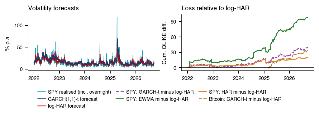

 MFM_ch9_intraday_day

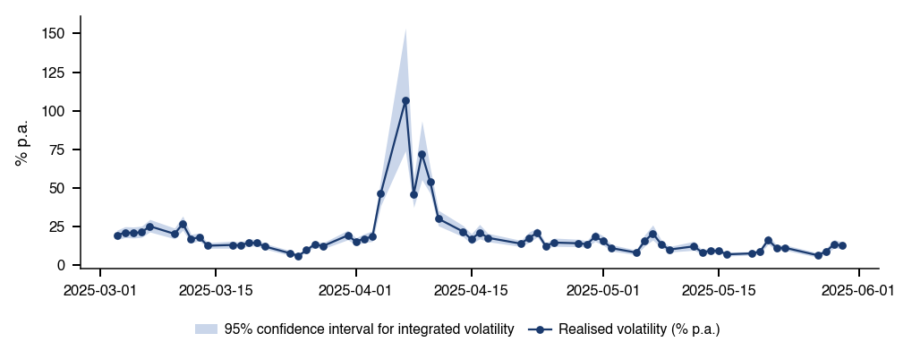
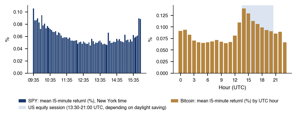
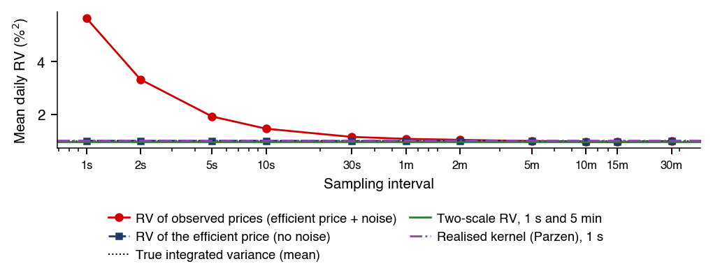

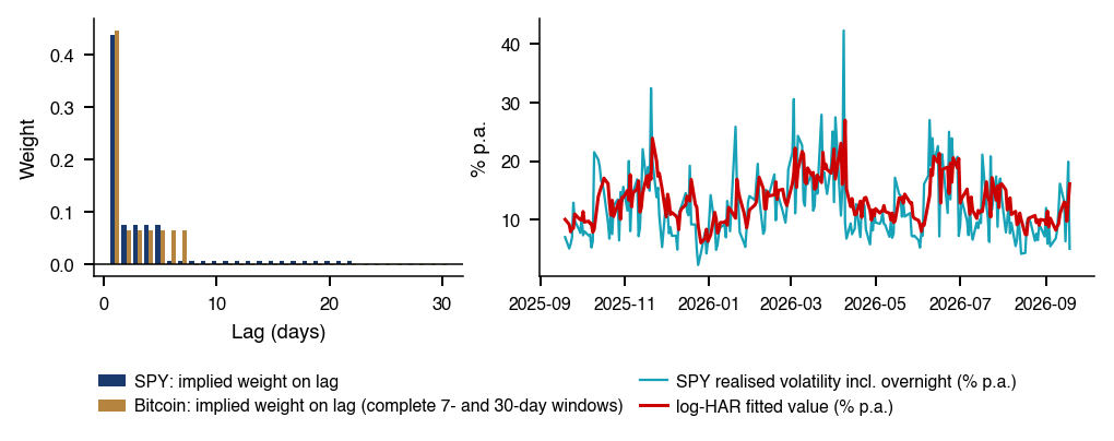
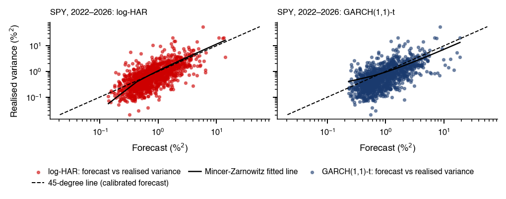
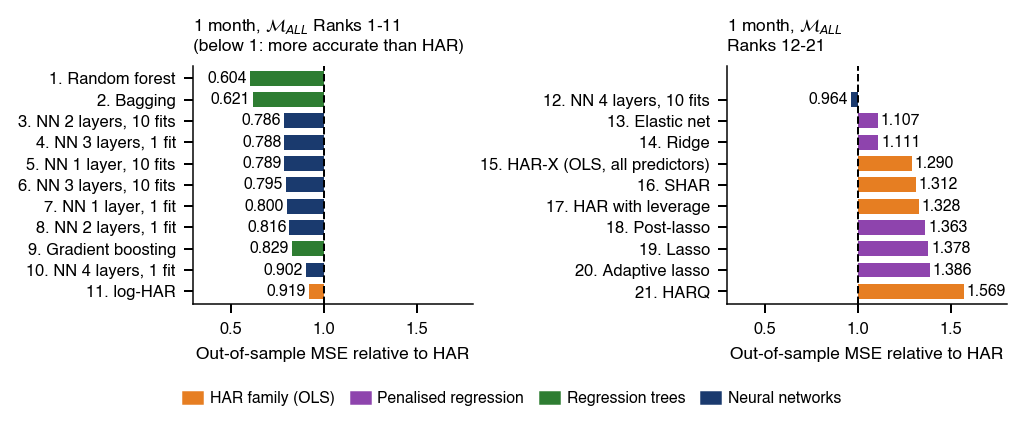
 Nonparametric and Semiparametric Models