Chapter 10: State space models, Kalman filter and Markov switching
Daniel Traian PELE
Bucharest University of Economic Studies IDA Institute Digital Assets Blockchain Research Center AI4EFin Artificial Intelligence for Energy Finance Romanian Academy, Institute for Economic Forecasting MSCA Digital Finance
The chapter asks how to measure a quantity that cannot be observed directly: the true level of a noisy series, the deviation of GDP from potential, a beta coefficient that changes over time, or a recession. The common answer is to write the unobserved quantity as a state and to let every new observation correct its estimate. The estimate is built recursively: in each period, the old estimate and the new observation are combined into an updated estimate.
The route has four stages. The first defines the state space form and shows that the local level, local linear trend and ARMA models and the regression with time-varying parameters are special cases of it. The second builds the Kalman filter, applies it by hand and uses it for smoothing, likelihood, missing values and forecasting. The third applies the method to the trend and cycle of Romanian GDP, discusses the Hodrick–Prescott filter and introduces dynamic factors. The fourth moves to discrete regimes with Markov-switching models. The chapter builds on the exponential smoothing of Chapter 0, the ARMA models of Chapter 2, the GARCH models of Chapter 5 and the long memory of Chapter 8.
In brief
Question: how do we measure what we cannot observe directly: the true level of a noisy series, the output gap, a changing beta, a recession?
the answer: write the unobserved quantity as a state and let the data update our estimate of it, period by period
Route of the chapter
the state space form: measurement and transition equations; local level, local linear trend, ARMA, time-varying regression
the Kalman filter by hand; smoothing; likelihood and estimation; missing values
trend and cycle: Romanian GDP, the HP filter and its critique; dynamic factors and nowcasting
Markov switching: recessions, Romanian growth regimes, volatility regimes
The first outcomes concern modelling and computation. The reader should be able to write a model in state space form, that is, to choose the state vector and the system matrices for a local level, a local linear trend, an AR(2) or a regression with a varying coefficient. The reader should then be able to run the Kalman filter by hand for a few periods, explain how the Kalman gain splits a surprise between signal and noise, and show that simple exponential smoothing is the steady-state Kalman filter of the local level model.
The empirical outcomes concern estimation and interpretation. The reader estimates the variances of a model by maximum likelihood, distinguishes the filtered from the smoothed estimate, handles missing values and builds forecasts with intervals. The reader decomposes GDP into trend and cycle, compares the Hodrick–Prescott filter with its alternatives and understands the critique of Hamilton (2018). Finally, the reader estimates a Markov-switching model and interprets the regime probabilities, their expected durations and the pitfalls of estimation.
In brief
Write a model in state space form: local level, local linear trend, AR(2), a regression with a time-varying coefficient
Run the Kalman filter by hand and explain the Kalman gain
Show that simple exponential smoothing is the steady state of the local level filter
Estimate a state space model by maximum likelihood, smooth it, and handle missing values and forecasts
Decompose GDP into trend and cycle and judge the HP filter against the critique of Hamilton (2018)
Estimate a Markov-switching model and read its regime probabilities, durations and pitfalls
The course textbook is Huang and Petukhina (2022), whose chapter on state space models and the Kalman filter covers the first part of the material. The standard reference for state space methods is Durbin and Koopman (2012), which is also the source of the Nile example used throughout the chapter; Harvey (1989) develops structural time series models, and Shumway and Stoffer (2017), Chapter 6, gives a more statistical presentation. For regime changes, the founding paper is Hamilton (1989);Hamilton (1994) covers the Kalman filter in Chapter 13 and regime changes in Chapter 22, and Kim and Nelson (1999) combine the two topics.
The computations are done in Python. A Kalman filter written out in numpy shows every step of the algorithm, and the statsmodels library provides production implementations: UnobservedComponents for trend–cycle models, SARIMAX for ARIMA models, DynamicFactor for dynamic factors, and MarkovRegression and MarkovAutoregression for regime-switching models. The chapter's Quantlets reproduce every chart, and the course notebook runs in Google Colab.
Many of the quantities that matter in economics and finance cannot be observed directly. The "true" level of a noisy series, the potential output of an economy, the sensitivity of one stock market to another, or whether the economy is in a recession are quantities we infer from data rather than read off it. Published statistics are imperfect measurements of these quantities: they contain noise, arrive with a delay and get revised.
This chapter treats the unobserved quantity as a state that evolves over time according to a known law, and the data as noisy measurements of it. The state space form writes both relations in one framework, and the Kalman filter updates the estimate of the state period by period as observations arrive. The same framework contains the ARMA models of Chapter 2, the exponential smoothing of Chapter 0, trend–cycle models, regressions with moving coefficients and models with common factors.
The last part of the chapter moves to a discrete state: a regime, such as recession or expansion, a calm market or a turbulent one. The Markov-switching models of Hamilton (1989) estimate in every period the probability of each regime. The applications use the flow of the Nile, the GDP of Romania and of the US, the BET index and the S&P 500.
Annual flow of the Nile at Aswan, 1871–1970, in \(10^8\) m³ (dots), the one-step prediction \(a_t\) (dashed line), the filtered level \(a_{t|t}\) of the local level model (solid line) and the 90% band of the filtered level.
What you will be able to do
Write a model in state space form: local level, local linear trend, AR(2) and a regression with a time-varying coefficient.
Apply the Kalman filter by hand and explain the role of the Kalman gain.
Show that simple exponential smoothing is the steady state of the filter of the local level model.
Estimate a state space model by maximum likelihood, smooth it, and handle missing values and forecasts.
Decompose GDP into trend and cycle and assess the Hodrick–Prescott filter in the light of the critique of Hamilton (2018).
Estimate a Markov-switching model and interpret the regime probabilities, the durations and the pitfalls.
Chapter plan
Hidden statesFrom the navigation of the Apollo missions to the unobserved quantities of economics and finance.
The state space formMeasurement and transition equations; local level, local linear trend, ARMA, regression with time-varying parameters.
The Kalman filterPrediction and update, the Kalman gain, an example by hand and the link with exponential smoothing.
Smoothing, likelihood and missing dataThe Rauch–Tung–Striebel smoother, the likelihood from prediction errors, diagnostics, gaps in the data and forecasting.
Trend, cycle and common factorsUnobserved components models, the HP filter and its critique, the Romanian output gap, a time-varying beta and a common factor.
Markov switchingMarkov chains, the Hamilton filter, US recessions, Romanian regimes and volatility regimes.
SummaryThe main ideas, the formulas and the self-assessment questions.
Hidden states
A hidden state is a quantity that drives the behaviour of the data but does not itself appear in the data. The idea comes from control engineering, where the position and velocity of a spacecraft are inferred from imperfect measurements. The section presents the origin of the Kalman filter and then the inventory of hidden states estimated in the chapter: the level of a series, the trend and cycle of GDP, a beta coefficient, a common factor and a regime.
Kalman (1960) proposed a recursive method for estimating a hidden state from noisy measurements. The method alternates two steps. First, the dynamic model predicts where the state should be in the next period. Then a new measurement arrives, and the prediction is corrected by a fraction of the difference between the measurement and what the model expected. The weight of this correction is called the Kalman gain, and it balances two sources of uncertainty: how uncertain the model's prediction is and how noisy the measurement is.
The first large-scale use was in space navigation. At NASA Ames, the filter was adapted for the navigation of the Apollo spacecraft: the state was the position and velocity of the craft, and the measurements were star sightings and radar data. The 1968 photograph shows Jim Lovell at the guidance and navigation station of Apollo 8.
In economics the logic is the same, but the state has another meaning. It may be the trend or the cycle of a series, a regression coefficient that changes, or the regime the economy is in, and the measurements are the published data. As in navigation, no single measurement reveals the state; it is revealed by the combination of the model and the sequence of measurements.
The table lists the observed series, the hidden state and the model used in this chapter. The annual flow of the Nile and monthly inflation have a background level that changes slowly, covered by period-to-period fluctuations; the model is the local level. Real GDP contains a trend and a deviation from trend, estimated with an unobserved components model. The returns of a stock index depend on the returns of another market through a beta coefficient that may change over time, modelled with a regression with time-varying parameters. Several indicators of economic activity share an unobserved factor, estimated with a dynamic factor model. GDP growth and stock returns pass through regimes, recession or expansion, calm or turbulent, described by Markov-switching models.
The essential difference between the first four examples and the last is the nature of the state. In the first four the state is continuous: a level, a trend or a coefficient can take any real value. For a continuous state with linear dynamics and Gaussian errors, the optimal filter is the Kalman filter. In the last example the state is discrete: the economy is either in one regime or in the other. For a discrete state that evolves as a Markov chain, the corresponding filter is the Hamilton filter.
The two filters share the same structure. Each predicts today's state from yesterday's information, then updates the prediction using today's observation \(y_t\). The Kalman filter carries a mean and a variance; the Hamilton filter carries a probability for each regime.
In brief
Observed series
Hidden state
Model in this chapter
Nile flow, monthly inflation
the underlying level
local level
real GDP
trend and output gap
unobserved components
stock index returns
a time-varying beta
time-varying regression
several activity indicators
one common factor
dynamic factor model
GDP growth, returns
recession or expansion; calm or turbulent
Markov switching
The first four have a continuous state and are filtered by the Kalman filter
The last has a discrete state (a regime) and is filtered by the Hamilton filter
Both filters do the same thing: predict the state, then update the prediction with \(y_t\)
Section summary
The quantities estimated in this chapter are hidden states: a level, a trend, a gap, a coefficient, a factor or a regime. All are handled the same way, through a model of how the state evolves, a model of how the state relates to the data, and a filter that alternates prediction and update. Continuous states are filtered with the Kalman filter, discrete states with the Hamilton filter.
The state space form
The state space form writes a time series model with two equations: one that says how the state generates the data and one that says how the state evolves. The section defines the general form, then builds the local level and local linear trend models in turn, writes ARMA models and the regression with time-varying parameters in this form, and shows the link with exponential smoothing. All these models differ only in the choice of the system matrices.
The first is the measurement equation. It links the observation \(y_t\), here a scalar, to the state vector \(\alpha_t\), of dimension \(m \times 1\), which is not observed. The row \(Z_t\), of dimension \(1 \times m\), holds known numbers that say which combination of the state is measured, and \(\varepsilon_t\) is the measurement noise, with variance \(H\). The second is the transition equation: the state evolves as a vector autoregression of order 1, VAR(1), of the kind studied in Chapter 6, with the \(m \times m\) matrix \(T\). The matrix \(R\) says how the state shocks \(\eta_t\) enter each component of the state, and \(Q\) is their variance matrix.
The model is completed by the initial state, \(\alpha_1 \sim N(a_1, P_1)\), where \(a_1\) and \(P_1\) are its mean and variance, and by the assumption that \(\varepsilon_t\),\(\eta_s\) and \(\alpha_1\) are mutually independent. The system matrices \(Z_t\),\(H\),\(T\),\(R\) and \(Q\) depend on a parameter vector \(\theta\), usually variances and autoregressive coefficients, which is estimated by maximum likelihood.
The advantage of this form is its generality. The same two equations, with other matrices, describe ARMA models, exponential smoothing, trend–cycle models, regressions with moving coefficients and factor models (Durbin and Koopman, 2012). Once a model is written in this form, the same Kalman filter computes the state estimate, the likelihood, the forecasts and the missing values.
\(y_t\): the observation (here a scalar); \(\alpha_t\): the state vector (\(m \times 1\)), not observed; \(Z_t\): a \(1 \times m\) row of known numbers
the state evolves as a first-order vector autoregression (VAR(1), Chapter 6); \(T\) is \(m \times m\)
\(R\): maps the shocks \(\eta_t\) into the state; \(H\), \(Q\): the variances of the measurement and of the state shocks
initial state: \(\alpha_1 \sim N(a_1, P_1)\), \(a_1\), \(P_1\): its mean and variance; \(\varepsilon_t\), \(\eta_s\) and \(\alpha_1\) mutually independent
The system matrices\(Z_t, H, T, R, Q\) contain the parameters \(\theta\); they are estimated by maximum likelihood
the same form covers ARMA, exponential smoothing, trend–cycle models, regressions with moving coefficients and factor models Durbin and Koopman (2012)
The state is the level \(\mu_t\), and all matrices are scalars: \(Z = T = R = 1\),\(H = \sigma^2_\varepsilon\) and \(Q = \sigma^2_\eta\). The two shocks play different roles. The measurement shock \(\varepsilon_t\) affects only the current observation and is gone in the next period. The level shock \(\eta_t\) moves the level permanently, because the level is a random walk.
The signal-to-noise ratio \(q = \sigma^2_\eta/\sigma^2_\varepsilon\) measures how much of the movement of the series is permanent. For \(q = 0\) the level is constant, and the series is white noise around a mean. As \(q\) grows without bound, the measurement noise becomes negligible and the series is a pure random walk. Between these extremes, the series has a moving level observed through noise.
The reduced form of the model shows the link with ARIMA models. The first difference is \(\Delta y_t = \eta_{t-1} + \varepsilon_t - \varepsilon_{t-1}\), a sum of white noises with no autocorrelation beyond lag 1, hence an MA(1) process. Its variance is \(\gamma(0) = \sigma^2_\eta + 2\sigma^2_\varepsilon\), and its first-order autocovariance is \(\gamma(1) = -\sigma^2_\varepsilon\), because \(\varepsilon_{t-1}\) enters \(\Delta y_t\) with a minus sign and \(\Delta y_{t-1}\) with a plus sign. This gives \(\rho(1) = -1/(q+2)\), a value between \(-1/2\) and 0. The local level model is therefore an ARIMA(0,1,1), of the kind studied in Chapter 3, with a negative MA coefficient.
In brief
Local level (random walk plus noise): \(y_t = \mu_t + \varepsilon_t\), \(\mu_{t+1} = \mu_t + \eta_t\)
state \(\alpha_t = \mu_t\), the level; \(Z = T = R = 1\), \(H = \sigma^2_\varepsilon\), \(Q = \sigma^2_\eta\)
\(\varepsilon_t\): measurement noise that disappears next period; \(\eta_t\): a permanent shift of the level
Signal-to-noise ratio\(q = \sigma^2_\eta/\sigma^2_\varepsilon\): how much of the movement is permanent
\(q = 0\): a constant level (white noise around a mean); \(q \to \infty\): a pure random walk
Reduced form: \(\Delta y_t = \eta_{t-1} + \varepsilon_t - \varepsilon_{t-1}\) is an MA(1) with \(\rho(1) = -1/(q+2)\)
so the local level model is an ARIMA(0,1,1) (Chapter 3) with a negative MA coefficient
\(\gamma(0) = \sigma^2_\eta + 2\sigma^2_\varepsilon\) and \(\gamma(1) = -\sigma^2_\varepsilon\) give \(\rho(1)\)
Question for the room What is F1, the variance of the first prediction error of the AR(2) filter?
Answer
0.858 = γ(0), the stationary variance of the AR(2), the (1,1) element of P1. F2 = 0.748, and from t = 3 on, with two lags known, Ft = σ̂² = 0.739. A stationary model needs no diffuse start.
Question for the room With T = 200, which path has the lag-1 autocorrelation of Δyt closest to −0.5?
Answer
The one with q = 0.01: −0.51 (theory −1/2.01 = −0.50); for q = 1 the autocorrelation is −0.28 (theory −1/3). When the noise dominates, Δyt ≈ εt − εt−1, an MA(1) with ρ(1) = −1/2; the first difference of a random walk without noise would be uncorrelated.
The left panel simulates three local level models with the same standard shocks \(\varepsilon_t\) and \(\eta_t\), with \(\sigma^2_\varepsilon = 1\) and with the signal-to-noise ratio \(q\) equal to 0.01, 0.1 and 1. Thin lines are the observations \(y_t\), thick lines the levels \(\mu_t\). Because the shocks are the same, the differences between the paths come only from the value of \(q\).
For \(q = 0.01\) (blue), the level stays close to 10 throughout the simulation, and the observations fluctuate around it. For \(q = 1\) (red), the level wanders between about 2 and 23, and the observations follow it closely. The intermediate value \(q = 0.1\) (green) gives a level that moves visibly, but much less than the noise around it.
The right panel shows a local linear trend model, defined in the next frame. The orange line is the level \(\mu_t\), the purple line the observations, and the dashed line the slope \(\beta_t\), read on the right axis. The slope is itself a random walk, so the growth rate of the level changes slowly: the level rises fast when the slope is high, around period 35, and almost stalls when the slope approaches zero, around period 100.
In brief
Left: the same shocks \(\varepsilon_t, \eta_t \sim N(0, 1)\) with \(\sigma^2_\varepsilon = 1\) and \(q = 0.01;\ 0.1;\ 1\) (thin: \(y_t\), thick: \(\mu_t\)). Right: a local linear trend, whose slope \(\beta_t\) is itself a random walk
The simulations show what \(q\) means for the look of a series. With a small \(q\), the level barely moves and the series looks like noise around a mean. With a large \(q\), the level dominates and the series resembles a random walk. The reduced form of the previous frame can be checked on the simulations: the first-order autocorrelation of the first difference is −0.51 for \(q = 0.01\), close to the theoretical value \(-1/2.01 = -0.50\), and −0.28 for \(q = 1\), close to the theoretical value \(-1/3\).
The local linear trend model produces periods of fast growth and of slow growth, because its slope changes slowly. This is the kind of trend used below for Romanian GDP: an economy does not grow at a constant rate, but neither does it change its growth rate abruptly from one quarter to the next.
The simulations also pose the central problem of the chapter. When we generate the data, we know which part of each observation is level and which is noise. In practice we see only \(y_t\). The Kalman filter answers the question "how much of the observed movement is level?" when the variances are given, and the likelihood picks the variances that describe the data best.
In brief
Small \(q\): the level hardly moves and \(y_t\) looks like noise around a mean; large \(q\): the level wanders and \(y_t\) follows it
first-difference autocorrelation: \(-\)0.51 for \(q = 0.01\) (theory \(-1/2.01\)) and \(-\)0.28 for \(q = 1\) (theory \(-1/3\))
The local linear trend has a slope that changes slowly: periods of fast and slow growth
this is the trend model we will use for GDP
The estimation problem: from \(y_t\) alone, how much is level and how much is noise? The Kalman filter answers it for given variances; the likelihood chooses the variances
The state now has two components, \(\alpha_t = (\mu_t, \beta_t)'\): the level and the slope, that is, the growth rate per period. The measurement equation reads only the level, so \(Z = (1,\ 0)\). The transition matrix \(T\) has first row \((1,\ 1)\), because tomorrow's level is today's level plus today's slope, and second row \((0,\ 1)\), because tomorrow's slope is today's slope plus a shock. The level and slope shocks are independent, with \(Q = \mathrm{diag}(\sigma^2_\eta, \sigma^2_\zeta)\).
Three special cases link the model to earlier chapters. If both state variances are zero, the level and slope are fixed, and the trend is linear and deterministic, \(\mu_1 + \beta_1 t\), as in Chapter 3. If only \(\sigma^2_\zeta = 0\), the slope is constant and the level is a random walk with drift \(\beta\). If only \(\sigma^2_\eta = 0\), the level receives no shocks of its own and the trend changes only its slope; this is the smooth trend, also called the integrated random walk, the model behind the Hodrick–Prescott filter of Section 5.
The model's forecast extends the last estimate of the level with the last estimate of the slope: \(\hat y_{T+h} = \hat\mu_T + h\hat\beta_T\). This is the state space version of Holt's method from Chapter 0, except that the smoothing weights are not chosen ad hoc but follow from the estimated variances.
In brief
Local linear trend: \(y_t = \mu_t + \varepsilon_t\), \(\mu_{t+1} = \mu_t + \beta_t + \eta_t\), \(\beta_{t+1} = \beta_t + \zeta_t\)
state \(\alpha_t = (\mu_t, \beta_t)'\): the level and the slope (the growth rate)
Every ARMA model can be written in state space form. For an AR(2), \(y_t = \phi_1y_{t-1} + \phi_2y_{t-2} + u_t\), the state keeps the last two values, \(\alpha_t = (y_t, y_{t-1})'\). The measurement equation reads the first component, \(y_t = (1,\ 0)\,\alpha_t\), without measurement noise (\(H = 0\)). The transition equation is
The first row reproduces the AR(2) equation, and the second only moves \(y_t\) into the "yesterday's value" slot. The matrix \(T\) is the companion matrix of Chapter 2; its eigenvalues are the inverses of the roots of the AR polynomial, so the process is stationary exactly when the eigenvalues lie inside the unit circle.
For an ARMA(1,1), \(y_t = \phi y_{t-1} + u_t + \theta u_{t-1}\), a convenient choice of state is \(\alpha_t = (y_t, \theta u_t)'\), with \(T\) having rows \((\phi,\ 1)\) and \((0,\ 0)\) and with \(R = (1,\ \theta)'\). The first row gives \(y_{t+1} = \phi y_t + \theta u_t + u_{t+1}\), exactly the ARMA(1,1) equation. In general, an ARMA\((p,q)\) needs a state of dimension \(m = \max(p, q+1)\).
The practical importance is that the Kalman filter computes the exact Gaussian likelihood of an ARMA model, even with missing values. For this, the initial state starts from the stationary distribution: \(P_1\) solves \(P = TPT' + RQR'\), with solution \(\mathrm{vec}(P_1) = (I - T \otimes T)^{-1}\mathrm{vec}(RQR')\), where \(\mathrm{vec}\) stacks the columns of a matrix and \(\otimes\) is the Kronecker product. This is how SARIMAX in statsmodels estimates the ARIMA models of Chapters 2–4.
The example uses the quarter-on-quarter growth of US real GDP from 1947 to 2019, that is, \(T = 291\) observations from the FRED database (Federal Reserve Economic Data). An AR(2) with intercept, estimated with SARIMAX, gives \(\hat\phi_1 = 0.319\),\(\hat\phi_2 = 0.111\) and shock variance \(\hat\sigma^2 = 0.739\). The implied mean growth is \(\hat\mu = 0.774\%\) per quarter, roughly 3.1% per year.
The same model can be run through the Kalman filter written out explicitly, with the matrices of the previous frame and with the stationary initial variance \(P_1\). The log-likelihood computed by this filter is −368.9157, and the one reported by SARIMAX is also −368.9157. The match is no accident: SARIMAX computes the likelihood exactly through this mechanism.
The prediction errors \(v_t\) of the filter are the one-step forecast errors of the AR(2) model: the difference between the growth observed in quarter \(t\) and its forecast from the previous quarter. Section 4 shows how the likelihood is built from these errors and their variances.
In brief
Data: US real GDP growth, quarter on quarter, 1947–2019 (\(T = 291\), FRED GDPC1)
AR(2) with a constant by SARIMAX: \(\hat\phi_1 = 0.319\), \(\hat\phi_2 = 0.111\), \(\hat\sigma^2 = 0.739\), mean \(\hat\mu = 0.774\%\) per quarter
Our own filter, with the state space matrices of the previous slide and the stationary \(P_1\)
log-likelihood: Kalman \(-\)368.9157; SARIMAX\(-\)368.9157: the same number
The prediction errors \(v_t\) of the filter are the one-step forecast errors of the AR(2); the likelihood is built from them (Section 4)
An ordinary regression assumes that the effect of \(x_t\) on \(y_t\) is the same over the whole period. The regression with time-varying parameters (TVP) drops this assumption and lets the coefficient evolve as a random walk:
The state is \((\alpha, \beta_t)'\). What is new compared with the earlier models is that the measurement row \(Z_t = (1,\ x_t)\) changes over time, because it contains the regressor. The state variance matrix is \(Q = \mathrm{diag}(0, \sigma^2_\eta)\): the intercept is fixed and the coefficient moves. If \(\sigma^2_\eta = 0\), the coefficient is constant, and the Kalman filter computes the ordinary least squares (OLS) estimator recursively, updating it with each new observation.
Economic examples abound: a market beta that rises in crises, an exchange-rate pass-through to inflation that changes with the monetary regime, an inflation persistence that falls after the adoption of inflation targeting. The usual alternative is a rolling-window regression. The TVP regression is better for three reasons: it does not require an arbitrary choice of window length, it uses all observations with weights set by the likelihood, and it gives a standard error for every \(\beta_t\).
Chapter 0 introduced simple exponential smoothing (SES): a level \(\ell_t\) is updated by the rule \(\ell_t = \alpha y_t + (1-\alpha)\ell_{t-1}\), and the forecast for the next period is \(\hat y_{t+1} = \ell_t\). Rewritten as \(\ell_t = \ell_{t-1} + \alpha(y_t - \ell_{t-1})\), the rule says that the new level is the old level plus a fraction \(\alpha\) of the surprise, that is, of the difference between the observation and the forecast.
This is exactly the form of a Kalman update. Muth (1960) showed that SES gives the optimal forecasts when the data follow the local level model. Section 3 shows that the weight \(\alpha\) is the steady-state Kalman gain of this model, so choosing \(\alpha\) amounts to an assumption about the signal-to-noise ratio.
The ETS models (error, trend, seasonality) of Hyndman et al. (2008) are also state space models, but with a single source of error: the same shock enters the observation and all the components. The models in this chapter have separate shocks for each component, such as \(\varepsilon_t\) and \(\eta_t\) in the local level model. Both families give the same point forecasts in the simple cases, but they differ in the interpretation of the components and in how they are estimated.
equivalently \(\ell_t = \ell_{t-1} + \alpha(y_t - \ell_{t-1})\): old level plus a share \(\alpha\) of the surprise
Muth (1960): SES gives the optimal forecasts when the data follow the local level model
Section 3 shows it: \(\alpha\) is the steady-state Kalman gain
ETS models (error, trend, seasonal) are state space models with a single source of error Hyndman et al. (2008); the models here have separate shocks for each component
The state space form (10.1) describes a hidden state that follows a VAR(1) and is observed with noise. In the local level model, the ratio \(q = \sigma^2_\eta/\sigma^2_\varepsilon\) fixes how much of the movement is permanent, and the reduced form is an ARIMA(0,1,1). The local linear trend, ARMA models and the TVP regression are other choices of the matrices \(Z_t\),\(T\) and \(Q\). The likelihood computed with the Kalman filter for an AR(2) equals the exact ARMA likelihood.
In brief
\(y_t = Z_t\alpha_t + \varepsilon_t\), \(\alpha_{t+1} = T\alpha_t + R\eta_t\): a hidden VAR(1) observed with noise
Local level: \(q = \sigma^2_\eta/\sigma^2_\varepsilon\); reduced form ARIMA(0,1,1)
Local linear trend, ARMA and TVP regression are other choices of \(Z_t, T, Q\)
The Kalman likelihood of an AR(2) equals the exact ARMA likelihood
Section summary
The state space form reduces a wide variety of models to the same pair of equations. The local level separates a permanent level from transitory noise, the local linear trend adds a slowly changing growth rate, ARMA models enter through the companion matrix, and the TVP regression lets a coefficient move. Exponential smoothing, in turn, is the updating rule of a local level model. The next step is the algorithm that estimates the state in all these models: the Kalman filter.
The Kalman filter
The Kalman filter computes, period by period, the best estimate of the state given the observations so far, together with the uncertainty of that estimate. The section presents the idea of the filter, the formulas of its two steps, the role of the Kalman gain, an example computed by hand and the steady state, which links the filter to exponential smoothing. The application is the flow of the Nile.
Write \(Y_t = (y_1, \dots, y_t)\) for all observations up to time \(t\). The filter tracks two estimates of the state. The prediction \(a_t = E(\alpha_t \mid Y_{t-1})\) is the estimate of today's state from the data up to yesterday, with variance matrix \(P_t\). The filtered estimate \(a_{t|t} = E(\alpha_t \mid Y_t)\) also uses today's observation, with variance \(P_{t|t}\).
Each period has two steps. In the update step, \(y_t\) arrives and the prediction \(a_t\) is corrected by a fraction of the surprise, that is, of the prediction error \(v_t = y_t - Z_ta_t\). In the prediction step, the filtered estimate passes through the transition equation and gives the prediction for the next period, \(a_{t+1}\). The cycle repeats until the end of the sample.
If the errors are Gaussian, \(a_{t|t}\) is the exact conditional mean of the state, hence the best estimate in the mean squared error sense. Without normality, the filter remains the best estimator that is linear in the data (Durbin and Koopman, 2012). The filter needs a starting point, \(a_1\) and \(P_1\). For a stationary state, the stationary distribution is used. For a nonstationary state, such as the level of a random walk, a diffuse initialisation is used: a very large \(P_1\), which means we know nothing about the initial state, so that the first observation determines the estimate almost entirely.
In brief
Notation: \(Y_t = (y_1, \dots, y_t)\); we track two numbers (vectors) for the state
prediction: \(a_t = E(\alpha_t \mid Y_{t-1})\) with variance \(P_t\)
filtered estimate: \(a_{t|t} = E(\alpha_t \mid Y_t)\) with variance \(P_{t|t}\)
Each period has two steps
update: \(y_t\) arrives; correct \(a_t\) by a share of the surprise \(v_t = y_t - Z_ta_t\)
prediction: push the filtered state through the transition equation to get \(a_{t+1}\)
With Gaussian errors, \(a_{t|t}\) is the exact conditional mean; without normality it is still the best linear estimate Durbin and Koopman (2012)
Start: \(a_1, P_1\); for a non-stationary state we use a diffuse start (\(P_1\) very large: we know nothing)
The prediction error \(v_t\) has variance \(F_t\), which adds the uncertainty about the state, \(Z_tP_tZ_t'\), to the measurement noise, \(H\). The Kalman gain \(K_t\) turns the surprise into a correction of the state, and the state variance falls after the observation. The prediction step then passes the filtered state through the transition equation:
For the local level model all quantities are scalars: \(F_t = P_t + \sigma^2_\varepsilon\),\(K_t = P_t/(P_t + \sigma^2_\varepsilon)\), and the two steps combine into \(a_{t+1} = a_t + K_t(y_t - a_t)\) and \(P_{t+1} = P_t(1 - K_t) + \sigma^2_\eta\). The level predicted for tomorrow is the level predicted for today plus a fraction \(K_t\) of today's surprise. If \(y_t\) is missing, the update step is skipped, \(a_{t|t} = a_t\) and \(P_{t|t} = P_t\), and the filter goes straight to the prediction.
In the local level model, the gain \(K_t = P_t/(P_t + \sigma^2_\varepsilon)\) is a number between 0 and 1, and the filtered estimate can be written as a weighted average: \(a_{t|t} = (1 - K_t)\,a_t + K_t\,y_t\). The gain is the weight given to the new observation, and \(1 - K_t\) is the weight of the model's prediction.
Two uncertainties compete. If the measurements are very noisy, \(\sigma^2_\varepsilon\) is large, the gain is small, and the filter trusts the model more than any single observation. If the state is very uncertain, \(P_t\) is large, for example at the start of the sample or after a run of missing values, the gain approaches 1, and the filter relies almost entirely on the data. The formula is the same as for combining two independent estimates of the same quantity, each weighted by its precision: the precision of the prediction is \(1/P_t\) and that of the observation is \(1/\sigma^2_\varepsilon\).
The state variance always falls after an observation, because \(P_{t|t} = (1 - K_t)P_t \le P_t\): any new information reduces uncertainty. In the prediction step the variance rises by \(\sigma^2_\eta\), because the level receives a new shock. The two forces balance: after a number of periods, the variance and the gain settle into a steady state.
In brief
Local level: \(K_t = \dfrac{P_t}{P_t + \sigma^2_\varepsilon}\) is the weight of the new observation, between 0 and 1
\(a_{t|t} = (1 - K_t)\,a_t + K_t\,y_t\): a weighted average of the prediction and the observation
Two uncertainties compete
noisy measurements (large \(\sigma^2_\varepsilon\)): small \(K_t\), trust the model
uncertain state (large \(P_t\), e.g. at the start or after missing data): large \(K_t\), trust the data
The variance always falls with an observation: \(P_{t|t} = (1 - K_t)P_t \le P_t\)
and grows by \(\sigma^2_\eta\) in the prediction step: the two forces settle at a steady state
The same formula as the weighting of two independent estimates by their precisions \(1/P_t\) and \(1/\sigma^2_\varepsilon\)
The example uses a local level model with \(\sigma^2_\varepsilon = 4\) and \(\sigma^2_\eta = 1\), so \(q = 0.25\). The initial estimate of the level is \(a_1 = 10\), with variance \(P_1 = 4\), and the data are \(y = (12, 11, 14)\).
In period 1, the variance of the prediction error is \(F_1 = P_1 + \sigma^2_\varepsilon = 4 + 4 = 8\), the gain is \(K_1 = 4/8 = 0.5\), and the surprise is \(v_1 = 12 - 10 = 2\). The filtered level is \(a_{1|1} = 10 + 0.5 \cdot 2 = 11\), with variance \(P_{1|1} = 4(1 - 0.5) = 2\). The prediction for period 2 keeps the level, \(a_2 = 11\), but adds the variance of the level shock: \(P_2 = 2 + 1 = 3\). Because the uncertainty of the prediction equalled the measurement noise, the observation and the prediction received equal weights.
In period 2, \(F_2 = 3 + 4 = 7\),\(K_2 = 3/7 = 0.429\), and the surprise is \(v_2 = 11 - 11 = 0\). The observation confirms the prediction, so the level does not change, \(a_{2|2} = 11\), but the uncertainty falls to \(P_{2|2} = 3 \cdot 4/7 = 1.71\). The prediction for period 3 is \(a_3 = 11\), with \(P_3 = 1.71 + 1 = 2.71\). The gain has fallen from 0.5 to 0.429: as the filter accumulates information about the level, it relies less on each new observation.
In brief
Local level with \(\sigma^2_\varepsilon = 4\), \(\sigma^2_\eta = 1\) (\(q = 0.25\)); prior \(a_1 = 10\), \(P_1 = 4\); data \(y = (12, 11, 14)\)
The table collects all the quantities of the filter over the three periods: the observation \(y_t\), the prediction \(a_t\) and its variance \(P_t\), the prediction error variance \(F_t\), the gain \(K_t\), the surprise \(v_t\), the filtered level \(a_{t|t}\) and its variance \(P_{t|t}\). Each row is computed from the previous one with formulas (10.3) and (10.4).
In period 3, \(P_3 = 2.71\), so \(F_3 = 6.71\) and \(K_3 = 2.71/6.71 = 0.404\). The surprise is \(v_3 = 14 - 11 = 3\), and the filtered level becomes \(a_{3|3} = 11 + 0.404 \cdot 3 = 12.21\), with variance 1.62. Although the observation is 3 units above the prediction, the level rises by only \(0.404 \cdot 3 = 1.21\): the filter treats the rest of the surprise as measurement noise.
The forecast for period 4 is \(a_4 = 12.21\), with state variance \(P_4 = 1.62 + 1 = 2.62\). The forecast of the observation \(y_4\) has a larger variance, \(P_4 + \sigma^2_\varepsilon = 6.62\), because the future observation will also contain its own noise. The gain keeps falling towards the steady-state value \(\bar K = 0.390\), which corresponds to the steady-state prediction variance \(\bar P = 2.56\).
In the local level model, the prediction variance \(P_t\) converges to a fixed value \(\bar P\) at which a full step of the filter no longer changes the variance: \(\bar P = \bar P(1 - \bar K) + \sigma^2_\eta\), with \(\bar K = \bar P/(\bar P + \sigma^2_\varepsilon)\). Substituting \(\bar K\) gives a quadratic equation in \(\bar P\), whose positive solution is
\[\begin{aligned} \bar P &= \sigma^2_\varepsilon\,\frac{q + \sqrt{q^2 + 4q}}{2},\\ \bar K &= \frac{\bar P}{\bar P + \sigma^2_\varepsilon}. \end{aligned}\]
(10.5)
For the previous example, \(q = 0.25\) gives \(\bar P/\sigma^2_\varepsilon = (0.25 + \sqrt{1.0625})/2 = 0.64\), so \(\bar P = 2.56\) and \(\bar K = 2.56/6.56 = 0.390\).
In the steady state the updating rule becomes \(a_{t+1} = a_t + \bar K(y_t - a_t) = \bar K y_t + (1 - \bar K)a_t\). This is exactly simple exponential smoothing with weight \(\alpha = \bar K\): exponential smoothing is the steady-state Kalman filter of a local level model (Muth, 1960). The relation can be inverted. An SES weight \(\alpha\) corresponds to the signal-to-noise ratio \(q = \alpha^2/(1 - \alpha)\), so a large weight indicates a level that moves a lot relative to the noise.
The state space version adds what exponential smoothing lacks: a likelihood from which \(q\) is estimated, forecast intervals based on estimated variances, and a natural treatment of missing values. In addition, at the start of the sample the filter's time-varying gain is larger than \(\bar K\) and adapts faster than a fixed SES weight.
In brief
For the local level model, \(P_t\) converges to the solution of \(\bar P = \bar P(1 - \bar K) + \sigma^2_\eta\) with \(\bar K = \bar P/(\bar P + \sigma^2_\varepsilon)\)
solution: \(\bar P = \sigma^2_\varepsilon\,\dfrac{q + \sqrt{q^2 + 4q}}{2}\), \(\bar K = \dfrac{\bar P}{\bar P + \sigma^2_\varepsilon}\)
example: \(q = 0.25\) gives \(\bar P/\sigma^2_\varepsilon = (0.25 + \sqrt{1.0625})/2 = 2.56/4\) and \(\bar K = 0.390\)
In the steady state: \(a_{t+1} = a_t + \bar K(y_t - a_t) = \bar K y_t + (1 - \bar K)a_t\)
this is SES with \(\alpha = \bar K\): exponential smoothing is the Kalman filter of a local level model Muth (1960)
Inverse map: an SES weight \(\alpha\) corresponds to \(q = \alpha^2/(1 - \alpha)\)
the state space version adds what SES lacks: a likelihood for \(q\), forecast intervals, missing values
The Nile: the Kalman filter of the local level model
Question for the room ▶ raises σ²ε. At σ²ε = 8 (with P1 = 4), what is K1?
Answer
K1 = 4/(4 + 8) = 0.333: with noisier measurements the filter relies less on the observation, and the filtered level stays closer to the prediction (a1|1 = 10.67 instead of 11).
Question for the room Set y3 = 18 (the surprise becomes 7 instead of 3). How far does the level move at t = 3?
Answer
By K3v3 = 0.404·7 = 2.83, to a3|3 = 13.83. The gain K3 = 2.71/6.71 = 0.404 does not depend on the data, only on P3 and σ²ε: a larger surprise moves the level proportionally, not to the observation.
Question for the room ▶ moves q from 0.01 to 10. What is K̄ at q = 10?
Answer
P̄/σ²ε = (10 + √140)/2 = 10.92, so K̄ = 10.92/11.92 = 0.916. K̄ stays below 1 for every finite q; q/(q + 1) = 0.909 is not the steady state.
Question for the room Cut the sample at 1920. Does q̂ rise or fall compared to the full sample?
Answer
It rises, to 0.163 (0.097 on 1871–1970), with σ̂²ε = 19103. Over 50 years the 1899 break weighs more, and the likelihood attributes it to movement of the level.
Question for the room ▶ takes q to 1. Where is the filtered level in 1899, the year with flow 774?
Answer
At 899, against 1037 at q̂ = 0.097: with q = 1, K̄ = 0.618, and the level takes almost two thirds of the surprise (757 in 1905). The level adapts to the dam faster, but it also follows isolated years.
The series is the annual flow of the Nile at Aswan from 1871 to 1970, in \(10^8\) m³: 100 observations, the classic example of Durbin and Koopman (2012). The variances of the local level model are estimated by maximum likelihood with a diffuse initialisation: the measurement noise variance is \(\hat\sigma^2_\varepsilon = 15100\), the level shock variance is \(\hat\sigma^2_\eta = 1468\), and the signal-to-noise ratio is \(\hat q = 0.097\). These are the estimates of Durbin and Koopman (2012).
The chart shows the annual flows as dots, the one-step prediction \(a_t\) as a dashed line and the filtered level \(a_{t|t}\) as a solid line, with the 90% band of the filtered level. Today's prediction is yesterday's filtered level, so the dashed line is the solid line shifted by one year. Individual flows scatter widely around the level: some years exceed 1250, others fall below 500, while the filtered level moves between about 750 and 1200.
The most visible feature of the chart is the fall of the level around 1900, from about 1150 to about 850, after which the level stays much lower until the end of the sample. The filter does not jump to the new level in one year; it comes down gradually as the weak years accumulate.
In brief
Annual flow at Aswan, 1871–1970 (\(10^8\) m\(^3\), statsmodels); variances by maximum likelihood with a diffuse start: \(\hat\sigma^2_\varepsilon = 15100\), \(\hat\sigma^2_\eta = 1468\), \(\hat q = 0.097\), the estimates of Durbin and Koopman (2012)
The signal-to-noise ratio \(\hat q = 0.097\) says that most of the year-to-year variation is noise: the variance of the level shock is about ten times smaller than the variance of the annual noise. The steady-state gain is \(\bar K = 0.267\), so each new flow moves the estimated level by about a quarter of the surprise. The statsmodels implementation, UnobservedComponents with the llevel specification, gives the variances 15078 and 1479; the model is the same, and the small difference comes from a slightly different treatment of the diffuse start.
The year 1899 shows the mechanism. The level predicted for 1899 was 1133 and the observed flow was 774, so the surprise was \(v = -359\). The filter lowers the level only to 1037, because it cannot tell from a single year whether the fall is noise or a permanent change. Only after several weak years does it accept the new level: in 1905 the filtered level reaches 834. The historical explanation is the construction of the first Aswan dam, completed in 1902.
At the end of the sample, in 1970, the filtered level is 798, with standard error 63. This is far below the mean of the whole sample, 919: the mean mixes the high level before 1899 with the low level afterwards, whereas the filter tracks the current level.
In brief
Most of the year-to-year movement is noise: \(\hat q = 0.097\), so each flow moves the level by about a quarter of the surprise (\(\bar K = 0.267\))
statsmodelsUnobservedComponents('llevel') gives 15078 and 1479: the same model, a slightly different start
1899: the flow is 774, the predicted level 1133; the surprise \(v = \ensuremath{-}359\) lowers the level only to 1037
the filter needs several low years to accept the new level (834 in 1905): the first Aswan dam was completed in 1902
In 1970 the level is 798 with standard error 63, well below the sample mean 919
Convergence of the Kalman gain and equivalence with SES
Question for the room ▶ takes q to 1. From which year on is Kt within 0.001 of K̄?
Answer
From year 5 (from year 11 at q̂ = 0.097 and from year 17 at q = 0.03). With a large q, Pt settles quickly: every new observation dominates the uncertainty left by the diffuse start.
The left panel shows the Kalman gain \(K_t\) of the Nile filter, year by year from 1872 to 1891, and the dashed line is the steady-state gain \(\bar K = 0.267\). After the diffuse start the first gain is large, because the filter knows almost nothing about the level; the gain then falls quickly and settles on the steady-state value.
The right panel compares two one-step forecasts over the whole period: the Kalman forecast \(a_t\) (red) and simple exponential smoothing with \(\alpha = \bar K = 0.267\), started from the first observation (green, dashed). The two lines overlap almost everywhere. Differences exist only in the first years, when the Kalman gain is still larger than \(\bar K\).
In brief
Left: \(K_t\) of the Nile filter; right: the Kalman one-step forecasts \(a_{t}\) and SES with \(\alpha = \bar K\), started at the first observation
The gain starts at 0.523 after the diffuse start, falls to 0.297 in year 5, and from year 11 on it is within 0.001 of the steady-state value \(\bar K = 0.267\). The Kalman and SES forecasts differ by 0.24 in year 5 and by less than 0.02 after 20 years, negligible amounts compared with flows in the hundreds. For a series of 100 years, the filter and SES are practically the same method.
The SES weight can also be chosen directly, as in Chapter 0, by minimising the sum of squared one-step forecast errors. For the Nile this gives \(\hat\alpha = 0.246\), which corresponds to the signal-to-noise ratio \(q = \alpha^2/(1-\alpha) = 0.080\). The result is close to the likelihood estimate, \(\hat q = 0.097\): two different criteria pick almost the same model.
The state space view also gives the SES weight an interpretation. The weight \(\alpha\) is large when the level moves a lot relative to the noise and small when the noise dominates. An \(\alpha\) of about a quarter, as for the Nile, describes a series in which each observation contains a lot of noise, but the level changes enough for the distant past to matter little.
In brief
\(K_t\) starts at 0.523 (after the diffuse start), 0.297 in year 5, and is within 0.001 of \(\bar K = 0.267\) from year 11 on
the forecasts differ by 0.24 in year 5 and by less than 0.02 after 20 years
SES fitted directly by least squares (Chapter 0) gives \(\hat\alpha = 0.246\), i.e. \(q = \alpha^2/(1-\alpha) = 0.080\)
close to the likelihood answer: two criteria, one model
The state space view explains SES: \(\alpha\) is large when the level moves a lot relative to the noise
The update step computes the prediction error \(v_t = y_t - Z_ta_t\), its variance \(F_t = Z_tP_tZ_t' + H\), the gain \(K_t = P_tZ_t'F_t^{-1}\) and the filtered estimate \(a_{t|t} = a_t + K_tv_t\). The prediction step computes \(a_{t+1} = Ta_{t|t}\) and \(P_{t+1} = TP_{t|t}T' + RQR'\). The gain weighs the data against the model and settles into a steady state. The steady-state local level filter is SES with \(\alpha = \bar K\); for the Nile, \(\bar K = 0.267\).
The gain weighs the data against the model; it settles at a steady state
Local level in steady state = SES with \(\alpha = \bar K\); Nile: \(\bar K = 0.267\)
Section summary
The Kalman filter alternates prediction and update, and its gain splits each surprise between signal and noise according to the relative variances of the state and the measurement. In the local level model the gain converges quickly to a steady-state value, and the steady-state filter is simple exponential smoothing. For the Nile, each new flow moves the level by about a quarter of the surprise, and the filter needs several years to accept the fall in level around 1900.
Smoothing, likelihood and missing data
The Kalman filter is only the first step. The same recursion, completed by a backward pass, gives the estimate of the state based on the whole sample. The filter's prediction errors give the likelihood, and hence the parameter estimates, and the residuals for diagnostics. Missing values and forecasts are handled by skipping the update step. The section presents these tools and applies them to the Nile series.
Filtering uses the information \(Y_t\), the past and the present: it is the estimate an analyst can make in real time. Smoothing uses the information \(Y_n\), the whole sample of size \(n\): the smoothed estimate \(\hat\alpha_t = E(\alpha_t \mid Y_n)\) also takes into account the observations after \(t\). Its variance \(V_t\) cannot exceed the variance of the filtered estimate, \(V_t \le P_{t|t}\), because it uses more information.
The Rauch–Tung–Striebel smoother (Rauch, Tung and Striebel, 1965) is a backward pass, run after the filter has gone through the whole sample, from \(t = n-1\) down to \(t = 1\):
The matrix \(J_t\) is the smoother gain: the weight with which the revision coming from the future, \(\hat\alpha_{t+1} - a_{t+1}\), corrects the filtered estimate. If the smoothed estimate of tomorrow's state differs from the prediction made today, the future data contain information about today's state. At \(t = n\) there is no future, so the smoothed and filtered estimates coincide.
The two estimates have different uses. The filtered state is used for real-time decisions and forecasting, because it contains only the information available at the time. The smoothed state is used for history: dating breaks, estimating past output gaps or reconstructing a series.
In brief
Filtering uses \(Y_t\) (the past and the present): the real-time estimate
smoothing uses \(Y_n\) (the whole sample): \(\hat\alpha_t = E(\alpha_t \mid Y_n)\), with variance \(V_t \le P_{t|t}\)
Question for the room Move the year to 1898. What is the difference between the filtered and the smoothed level?
Answer
Filtered 1133, smoothed 1000: a difference of 134, larger than in 1897 (1145 against 1038, i.e. 107). The smoother uses the low years after 1899, so it lowers the level before the drop appears in the data.
Question for the room Set q = 0.001 (an almost constant level). What does the smoothed level look like around 1899?
Answer
Almost a straight line, falling slowly from 956 in 1897 to 881 in 1950: the step disappears. With a small q the model attributes the drop to noise, and the smoother cannot show a break that the model rules out.
The chart shows the annual flows of the Nile, the filtered level \(a_{t|t}\) (thin line) and the smoothed level \(\hat\alpha_t\) (thick line), with the 90% band of the smoothed level. Both estimates use the same maximum likelihood variances; only the information used differs.
The smoothed level is visibly smoother than the filtered one. The filter reacts to every unusual year, because it does not yet know whether the surprise will persist; the smoother sees the following years and can tell an isolated year from a lasting change. The 90% band of the smoothed level is narrower in the middle of the sample than at the ends, where information from the future or from the past is missing.
In brief
Filtered level \(a_{t|t}\) and smoothed level \(\hat\alpha_t\) with its 90% band; the same maximum-likelihood variances
The smoothed level starts to fall before the drop appears in the data. In 1897 the smoothed level is already 1038, whereas the filtered level is 1145. The smoother uses the weak years after 1898, so it attributes part of the fall to the preceding years as well. This property is useful for history but impossible in real time: in 1897 nobody knew the flows of the following years.
In 1900 the smoothed level is 920 and the filtered level 985. The smoothed level adapts faster to the new regime because it sees the run of weak years after 1900, which the filter discovers one at a time. The gain in precision shows in the standard errors: in 1920 the standard error of the smoothed level is 48, against 63 for the filtered level.
The smoothed path shows a step around 1899 more clearly than any moving average of Chapter 0. The advantage is not only visual: the smoother's weights follow from the estimated variances, and the estimate comes with an uncertainty band.
In brief
The smoothed level reacts to the 1898–1899 drop before it happens in the data: in 1897 it is already 1038, against 1145 filtered
it knows the future: useful for history, impossible in real time
In 1900: smoothed 920, filtered 985; the smoothed level adapts faster because it sees the low years after 1900
standard error in 1920: 48 smoothed against 63 filtered
The smoothed path shows a step near 1899 more clearly than any moving average of Chapter 0
The joint density of the observations can be written as a product of one-step conditional densities: \(p(y_1, \dots, y_n) = \prod_t p(y_t \mid Y_{t-1})\). With Gaussian errors, each conditional density is Normal, \(y_t \mid Y_{t-1} \sim N(Z_ta_t, F_t)\), and its mean and variance are exactly the quantities computed by the filter. This gives the prediction error decomposition:
Here \(\theta\) collects the model's parameters, for example the variances, and \(v_t\) and \(F_t\) are the prediction errors and their variances, computed by the filter for that value of \(\theta\). The term \(v_t^2/F_t\) penalises prediction errors that are large relative to their variance, and \(\log F_t\) penalises large variances: a good model predicts well and with justified confidence.
The computation is simple: one run of the filter gives \(\log L\) for one value of \(\theta\), and a numerical optimiser searches for the value that maximises it. With a diffuse initialisation, the first \(d\) terms of the sum are dropped, because there \(F_t\) is huge; for the local level model \(d = 1\), because a single observation pins down the level (Durbin and Koopman, 2012). The idea is the same as for the exact ARMA likelihood of Chapter 2, now valid for any state space model.
In brief
The joint density factorises into one-step conditional densities: \(p(y_1, \dots, y_n) = \prod_t p(y_t \mid Y_{t-1})\)
with Gaussian errors, \(y_t \mid Y_{t-1} \sim N(Z_ta_t, F_t)\): the filter delivers the mean and the variance
Variances must be positive, so the optimisation is carried out over \(\log\sigma^2\), which can take any real value. The likelihood surface can be flat in some directions, so it is prudent to start the optimisation from several initial values. A variance estimated at zero is common and has a clear interpretation: that component is deterministic. For example, a slope variance equal to zero means that the slope of the trend is constant.
For the local level model the likelihood can be concentrated. Write \(\sigma^2_\eta = q\sigma^2_\varepsilon\) and run the filter with \(\sigma^2_\varepsilon = 1\); for fixed \(q\), the noise variance then has a closed-form estimate, \(\hat\sigma^2_\varepsilon = \frac{1}{n-1}\sum_t v_t^2/F^*_t\), with the sum over the \(n - 1\) non-diffuse terms. Substituting this estimate into the likelihood, the profile log-likelihood depends only on \(q\) and can be plotted, as in the next frame.
The standard errors of the estimates come from the numerical Hessian of the log-likelihood. Competing models are compared with the AIC and BIC information criteria, and the adequacy of a model is checked on the standardised prediction errors \(e_t = v_t/\sqrt{F_t}\). The UnobservedComponents, SARIMAX and DynamicFactor classes of statsmodels all use this mechanism.
In brief
Optimise over \(\log\sigma^2\) (variances stay positive); several starting values, since the surface can be flat
a variance estimated at zero is common and meaningful: that component is deterministic
Concentrating: for the local level, write \(\sigma^2_\eta = q\sigma^2_\varepsilon\); for fixed \(q\), \(\hat\sigma^2_\varepsilon = \frac{1}{n-1}\sum_t v_t^2/F^*_t\) in closed form, with \(v_t\), \(F^*_t\) from the filter run with \(\sigma^2_\varepsilon = 1\), \(\sigma^2_\eta = q\)
the profile log-likelihood is then a function of \(q\) alone (next chart)
Standard errors from the numerical Hessian; model choice by AIC and BIC; tests on the standardised prediction errors \(e_t = v_t/\sqrt{F_t}\)
statsmodels: UnobservedComponents, SARIMAX, DynamicFactor all use this machinery
Question for the room At q̂ = 0.097, which year contributes the most negative term to log L?
Answer
1913 (ℓt = −9.78), a single very dry year; then 1916 (−9.18) and 1899 (−9.02). The year 1871 is not in the sum: the diffuse start gives it a huge Ft.
Question for the room Take the chosen q to 10. What is the likelihood-ratio statistic against the maximum?
Answer
23.3, as far from the data as q = 0.001 (23.1); q = 1 gives 7.2. A level that chases every flood predicts one step ahead as badly as an almost constant level.
The left panel shows the profile log-likelihood of the local level model for the Nile as a function of the signal-to-noise ratio \(q\), on a logarithmic horizontal axis from \(10^{-4}\) to \(10\). The curve has a single maximum, at \(\hat q = 0.097\), marked by the dashed vertical line, and falls off on both sides.
The right panel shows what three values of \(q\) mean for the filtered level. With \(q = 0.001\) (green), the level is almost constant and declines very slowly, missing the fall around 1900. With \(q = 1\) (purple), the level follows almost every observation, including isolated extreme years. With the maximum likelihood value, \(q = 0.097\) (red), the level adapts to the lasting fall but not to every unusual year.
In brief
Left: profile log-likelihood of the Nile local level model against \(q\) (log scale); right: filtered levels for \(q = 0.001\), the ML value and \(q = 1\)
The maximum is clear, at \(\hat q = 0.097\), and the closed-form noise variance is \(\hat\sigma^2_\varepsilon = 15100\). The likelihood ratio statistic is twice the difference between the maximised log-likelihood and that of an alternative. Against \(q = 0.001\), an almost constant level, the statistic is 23.1; against \(q = 1\), it is 7.2. Compared with the 5% critical value of the \(\chi^2(1)\) distribution, 3.84, both alternatives are rejected, the first by a much wider margin.
The right panel of the previous chart explains why. A small \(q\) produces an almost flat level that misses the fall after 1899, so the forecasts for the years after 1900 are systematically too high. A large \(q\) produces a level that follows every flood, so the forecasts carry over last year's noise. The likelihood picks the compromise that predicts best one step ahead, because it is built exactly from the one-step prediction errors.
Choosing \(q\) is equivalent to choosing the SES weight \(\alpha\) of Chapter 0. The difference is that the choice now has a statistical criterion, the likelihood, which allows tests and confidence intervals.
In brief
A clear maximum at \(\hat q = 0.097\), with \(\hat\sigma^2_\varepsilon = 15100\) from the closed form
likelihood-ratio statistic against \(q = 0.001\) (an almost constant level): 23.1; against \(q = 1\): 7.2
Small \(q\): the level is almost flat and misses the drop after 1899; large \(q\): the level chases every flood
the likelihood picks the compromise that predicts best one step ahead
Choosing \(q\) is the same as choosing the SES weight \(\alpha\) in Chapter 0, now with a statistical criterion
If the model is correctly specified, the standardised prediction errors \(e_t = v_t/\sqrt{F_t}\) are independent and identically distributed (i.i.d.) with the standard Normal distribution. The checks are those of Chapters 1–2: the ACF and the Ljung–Box test for independence, the Jarque–Bera test for normality, and the time plot for extreme values.
State space models also offer a specific tool: the auxiliary residuals of Durbin and Koopman (2012). These are the smoothed disturbances \(\hat\varepsilon_t\) and \(\hat\eta_t\), that is, the estimates of the measurement shocks and the level shocks based on the whole sample, standardised by their standard deviations. Each type of residual detects a different problem. A large \(\hat\varepsilon_t\) points to an outlier in a single observation. A large \(\hat\eta_t\) points to a structural break in the level, a permanent shift.
The auxiliary residuals are computed by a backward recursion after the filter, called the disturbance smoother. They answer a question the prediction errors cannot separate: a large prediction error may come from an extreme year or from the start of a level shift.
In brief
If the model is right, the standardised prediction errors \(e_t = v_t/\sqrt{F_t}\) are i.i.d. \(N(0, 1)\)
the checks of Chapters 1–2: the ACF and the Ljung–Box test (independence), Jarque–Bera (normality), a plot over time (outliers)
Auxiliary residualsDurbin and Koopman (2012): the smoothed disturbances \(\hat\varepsilon_t\) and \(\hat\eta_t\), standardised
a large \(\hat\varepsilon_t\): an outlier in one observation
a large \(\hat\eta_t\): a break in the level, a permanent shift
Computed by a backward recursion (the disturbance smoother) after the filter
Question for the room Set q = 0.001. Is the Ljung–Box Q(10) test still passed?
Answer
No: Q(10) = 20.9, p = 0.022. An almost constant level leaves the drop after 1899 in the prediction errors, which become autocorrelated; at q̂ = 0.097, p = 0.21.
The left panel shows the standardised one-step prediction errors \(e_t\), and the right panel the standardised auxiliary residual of the level, \(\hat\eta_t\), where the bar in year \(t\) refers to the shock between year \(t\) and year \(t+1\). The dotted lines mark \(\pm 1.96\), the 95% limits of a standard Normal variable.
The prediction errors look like white noise: the bars alternate without a visible pattern, and only a few cross the limits. The level residual looks different. Around 1898 there is a cluster of large negative bars, several below −1.96, while elsewhere the bars mostly stay inside the limits. Auxiliary residuals of neighbouring years are correlated, so a single break shows up as a cluster of bars, with the largest at the time of the break.
In brief
Left: standardised one-step prediction errors \(e_t\); right: standardised auxiliary residual of the level, \(\hat\eta_t\) (a shock between year \(t\) and \(t+1\)); dashed: \(\pm 1.96\)
The tests on the prediction errors find no problems. The Ljung–Box statistic for 10 lags is \(Q(10) = 13.2\), with p-value 0.21, so it does not separate the autocorrelation from noise. The Jarque–Bera statistic is 0.05, with p-value 0.98, so it does not reject normality. Only 4 of the 99 standardised errors lie outside \(\pm 1.96\), whereas about 5 are expected for a standard Normal variable. The one-step errors give no evidence against the model.
The auxiliary residuals, however, locate two events. The level residual reaches its minimum in 1898, at −3.23: the level shock between 1898 and 1899, the permanent shift of the level. The observation residual reaches its minimum in 1913, at −3.04: a single very dry year, an outlier that does not change the level. Separating the two is exactly what the prediction errors cannot do.
The break of 1898–1899 is the same one that, in Chapter 8, made the Nile series look like a long-memory series. There, the break was an alternative explanation for slowly decaying autocorrelations; here, the model locates it on its own, in the year it happened.
Missing values are simple to handle in the Kalman filter. If \(y_t\) is missing, the update step is skipped and the prediction is made directly from the previous prediction: \(a_{t+1} = Ta_t\) and \(P_{t+1} = TP_tT' + RQR'\). The state variance grows in every period without data. In the likelihood, the term of the missing period is simply dropped. No interpolation by hand is needed.
Forecasting is the same mechanism. The \(h\)-step forecast from the end of the sample means treating \(y_{n+1}, \dots, y_{n+h}\) as missing values. For the local level model the forecast is the same at every horizon, \(\hat y_{n+h} = a_{n+1}\), because the best estimate of a future random walk is its current level. The forecast variance is \(P_{n+1} + (h-1)\sigma^2_\eta + \sigma^2_\varepsilon\): the uncertainty about today's level, plus the level shocks accumulated up to the horizon, plus the noise of the future observation.
The mechanism has many practical uses: irregular data, for example because of holidays, series that start at different dates, mixed frequencies such as monthly and quarterly data in one model, and the ragged edge of a nowcast. The smoother fills the gaps with the estimate \(\hat\alpha_t\) and the corresponding standard error.
In brief
A missing \(y_t\): no update; \(a_{t+1} = Ta_t\), \(P_{t+1} = TP_tT' + RQR'\)
the likelihood simply skips that term; nothing is interpolated by hand
Question for the room Gaps of 10 years (1891–1900 and 1931–1940): what is the standard error of the smoothed level in 1895?
Answer
78, against 99 in 1900 with 20-year gaps and 48 with all data. The band grows with the distance to the nearest observed year.
The left panel reproduces the experiment of Durbin and Koopman (2012): the years 1891–1910 and 1931–1950 are removed from the Nile series, 40 years in total, and the model is smoothed on the remaining data. The shaded bands mark the missing years, the red line is the smoothed level, and the pink area is its 90% band.
The right panel treats the years 1971–2000 as missing values, so it shows forecasts for 30 years after the end of the sample. The green line is the forecast, and the green area is the 90% forecast interval for the flow \(y\), not just for the level. The interval widens with the horizon.
In brief
Left: 1891–1910 and 1931–1950 removed (the experiment of Durbin and Koopman (2012)), smoothed level with 90% band; right: forecasts for 1971–2000 with 90% intervals for \(y\)
Inside a gap, the smoothed level is a straight line between the estimates at the two edges: without observations, the best estimate of a random walk between two known points is linear interpolation. The uncertainty band widens towards the middle of the gap and narrows near the observed years. In 1900, in the middle of the first gap, the standard error of the smoothed level is 99, against 48 with all the data.
The forecasts are constant at 798, the filtered level of 1970: a random-walk level has no predictable direction. The uncertainty, however, grows with the horizon. The standard error of the forecast flow is 144 one year ahead and 251 after 30 years. The difference comes from the accumulated level shocks, \((h-1)\sigma^2_\eta\), since the annual noise \(\sigma^2_\varepsilon\) is the same at every horizon.
Interior gaps, forecasts and parameter estimation are handled by the same code, by skipping the update step. This is one of the main practical advantages of state space models over methods that require a complete series.
In brief
Inside a gap the smoothed level is a straight line between the two edges; its standard error grows to 99 in 1900, against 48 with all data
the band widens towards the middle of the gap and narrows near observed years
Forecasts are flat at 798: a random-walk level has no predictable direction
standard error of \(y\): 144 one year ahead, 251 after 30 years
The same code handles missing data, forecasts and estimation: one of the main practical strengths of state space models
The filtered estimate is the real-time estimate; the smoothed estimate, from the RTS smoother, uses the whole sample and has a smaller variance. The log-likelihood (10.6) is built from the prediction errors and maximised numerically. Diagnostics use the standardised errors \(e_t\), and the auxiliary residuals find outliers and breaks, such as the Nile break of 1898–1899. Missing values and forecasts are handled by skipping the update step.
In brief
Filtered: real time; smoothed (RTS): the whole sample, smaller variance
Diagnostics on \(e_t\); auxiliary residuals find outliers and breaks (Nile 1898–1899)
Missing data and forecasts: skip the update step
Section summary
The filter, the smoother and the likelihood form a single toolkit. The filter gives the real-time estimate and the prediction errors; the smoother revises the estimate with information from the future; the likelihood, built from the prediction errors, chooses the variances. For the Nile, the likelihood picks \(\hat q = 0.097\), the diagnostics find no problems in the one-step errors, the auxiliary residuals separate the level break of 1898 from the extreme year 1913, and the gaps and forecasts are handled by the same mechanism.
Trend, cycle and common factors
The section applies state space methods to three problems in macroeconomics and finance. The first is the decomposition of GDP into trend and cycle, with an unobserved components model, the Hodrick–Prescott filter and the regression filter of Hamilton (2018), on Romanian data. The second is a time-varying beta between the Romanian stock market and the euro area. The third is a common factor of US economic activity, estimated from a dynamic factor model.
The structural time series model, also called the unobserved components (UC) model, of Harvey (1989) decomposes the series into components with a direct interpretation:
The components are the trend \(\mu_t\), modelled as a local level or a local linear trend, the cycle \(\psi_t\), the seasonal \(\gamma_t\) and the irregular component \(\varepsilon_t\). The decomposition resembles the one in Chapter 0, but there the components were extracted with fixed rules; here each component is a stochastic process with its own variance, estimated from the data.
The cycle can be modelled as a stationary AR(2), \(\psi_t = \phi_1\psi_{t-1} + \phi_2\psi_{t-2} + \kappa_t\), where \(\phi_1\) and \(\phi_2\) are the autoregressive coefficients and \(\kappa_t\) is the cycle shock. An alternative is a damped stochastic cycle with frequency \(\lambda_c\), in radians, hence with period \(2\pi/\lambda_c\). An AR(2) with complex roots also produces oscillations, which makes it suitable for business cycles.
For log GDP, the cycle \(\psi_t\) is the output gap: the percentage deviation of output from trend, interpreted as potential output. A positive gap indicates an economy producing above potential, with the risk of overheating; a negative one indicates idle resources. In Python the model is estimated with UnobservedComponents, with the specification level='smooth trend' and autoregressive=2, and the whole state is estimated with the Kalman filter and smoother.
In brief
Structural time series or unobserved components (UC) model Harvey (1989): \(y_t = \mu_t + \psi_t + \gamma_t + \varepsilon_t\)
trend \(\mu_t\) (local level or local linear trend), cycle \(\psi_t\), seasonal \(\gamma_t\), irregular \(\varepsilon_t\)
the decomposition of Chapter 0, but each component is a stochastic process with its own variance
The cycle: a stationary AR(2) \(\psi_t = \phi_1\psi_{t-1} + \phi_2\psi_{t-2} + \kappa_t\), or a damped stochastic cycle with period \(2\pi/\lambda_c\)
\(\phi_1\), \(\phi_2\): the AR coefficients of the cycle; \(\kappa_t\): the cycle shock; \(\lambda_c\): the frequency of the cycle, in radians
for log GDP, \(\psi_t\) is the output gap: the percentage deviation of output from its trend (potential)
In Python: UnobservedComponents(y, level='smooth trend', autoregressive=2); the whole state is estimated by the Kalman filter and smoother
where \(\Delta^2\tau_t = \tau_t - 2\tau_{t-1} + \tau_{t-2}\) is the change in the slope of the trend and \(\lambda \ge 0\) is the smoothing parameter. The first term asks the trend to stay close to the data, the second asks its slope to change little. For \(\lambda = 0\) the trend is the series itself; as \(\lambda\) grows without bound, the slope can no longer change and the trend becomes a straight line. For quarterly data the conventional value is \(\lambda = 1600\).
Harvey and Jaeger (1993) showed that the HP trend is exactly the smoothed trend of a particular UC model: a smooth trend whose second difference is white noise with variance \(\sigma^2_\zeta\), plus a white-noise irregular with variance \(\sigma^2_\varepsilon\), with \(\lambda = \sigma^2_\varepsilon/\sigma^2_\zeta\). The HP filter thus fixes two things that a UC model would estimate: the ratio of the variances and the assumption that the deviation from trend is white noise, without dynamics of its own.
Being a smoother, the HP filter uses future data. The trend in a given quarter depends on the observations after it, so the last values of the trend and the gap are revised as new quarters arrive. The problem is most serious precisely at the end of the sample, where economic policy decisions are made.
In brief
Hodrick and Prescott (1997): the trend \(\tau_t\) minimises \(\sum_t(y_t - \tau_t)^2 + \lambda\sum_t(\Delta^2\tau_t)^2\); \(\lambda = 1600\) for quarterly data
\(\Delta^2\tau_t = \tau_t - 2\tau_{t-1} + \tau_{t-2}\): the change in the slope of the trend; \(\lambda \ge 0\): the smoothing parameter
large \(\lambda\): a straight-line trend; \(\lambda = 0\): the trend is the series itself
This is exactly the smoothed trend of a UC model: smooth trend (\(\Delta^2\mu_{t+1} = \zeta_{t-1}\)) plus white noise, with \(\lambda = \sigma^2_\varepsilon/\sigma^2_\zeta\)Harvey and Jaeger (1993)
the HP filter imposes the signal-to-noise ratio and a white-noise gap; the UC model estimates both
Being a smoother, HP uses future data: its last values are revised as new quarters arrive
Hamilton (2018): why you should never use the HP filter
Hamilton (2018) raises three objections. First: applied to a random walk, which has no cycles, the HP filter produces a gap with regular cycles. The dynamics of the gap are created by the filter, not by the data. Second: the end of the sample is treated differently from the middle, because at the end the filter has no future data; hence the large revisions and the misleading real-time gaps. Third: the value \(\lambda = 1600\) is a convention, far from the value a likelihood would choose for typical macroeconomic series.
Hamilton's alternative is the regression filter. One estimates by OLS the regression of \(y_{t+h}\) on a constant and on \(y_t, y_{t-1}, y_{t-2}, y_{t-3}\), with \(h = 8\) quarters for quarterly data. The cycle is the regression residual: the part of today's value that could not be predicted two years earlier. The filter is one-sided by construction, because it uses only earlier data, so today's estimate is not revised when new data arrive, apart from re-estimation of the coefficients.
The output gap is never observed, so no method can be checked against the true value. What can be done is a comparison between methods, with the assumptions of each in plain view. The following frames compare the UC model, the HP filter and the Hamilton filter on Romanian GDP.
Question for the room ▶ takes λ to 100000. What becomes of the standard deviation of the HP gap?
Answer
5.5, against 2.9 at λ = 1600 and 1.3 at λ = 1: a stiffer trend leaves more of the movement of GDP in the gap.
Question for the room Which λ of the grid brings the HP trend closest to the UC trend?
Answer
λ = 400: the largest distance is 0.63 points (1.01 at λ = 100 and 2.65 at λ = 1600). The UC trend is more flexible than the trend imposed by λ = 1600, so a smaller λ approximates it better.
The series is \(100 \times \log\) of Romania's quarterly real GDP, seasonally and calendar adjusted, in chain-linked volumes, from the first quarter of 1995 to the second quarter of 2026, that is, \(T = 126\) quarters from the Eurostat database. Multiplying the logarithm by 100 makes differences read directly as approximate percentage changes. The UC model has a smooth trend and an AR(2) cycle; the HP filter uses \(\lambda = 1600\).
The chart shows the series (blue), the smooth trend of the UC model, estimated by smoothing (red), and the HP trend (green, dashed). The series declines slightly until 1999, rises quickly from 2000 to 2008, drops sharply in 2009, stagnates for a few years and resumes growth after 2013, with a visible drop in 2020. The two trends pass through the middle of these movements and almost overlap.
In brief
\(100 \times \log\) of real GDP, quarterly, seasonally and calendar adjusted, chain-linked volumes (Eurostat namq_10_gdp), 1995Q1–2026Q2 (\(T = 126\)); UC model: smooth trend plus AR(2) cycle; HP with \(\lambda = 1600\)
The trend grows on average by 2.5% per year. The path has a slow start, marked by the 1997–1999 recession, a boom until 2008, stagnation after the financial crisis and a recovery after 2013. The UC trend and the HP trend are almost identical; the difference between the methods lies not in the trend but in the deviation from it, where a small difference in trend becomes a relatively large difference in the gap.
The UC estimates describe how flexible the trend is. The variance of the slope shocks is \(\hat\sigma^2_\zeta = 0.078\). The AR(2) cycle has coefficients \(\hat\phi_1 = 0.61\) and \(\hat\phi_2 = -0.13\) and shock variance \(\hat\sigma^2_\kappa = 5.27\), and the variance of the irregular component is estimated at zero, so all variation around the trend is attributed to the cycle.
The ratio of the cycle shock variance to the slope shock variance is \(5.27/0.078 = 68\), far below the value 1600 that the HP filter imposes on the corresponding ratio. The comparison is approximate, because in the HP model the gap is white noise while here it is an AR(2), but the direction is clear: the data prefer a more flexible trend than the one imposed by HP. A more flexible trend absorbs part of the boom and of the recessions, so the UC gap will be smaller than the HP gap.
In brief
Average growth 2.5% per year, with a slow start (the 1997–1999 recession), a boom until 2008, a stagnation and a recovery after 2013
the two trends are almost identical: the difference between methods lies in the gap, not in the trend
UC estimates: \(\hat\sigma^2_\zeta = 0.078\) (trend slope), cycle AR(2) with \(\hat\phi_1 = 0.61\), \(\hat\phi_2 = \ensuremath{-}0.13\), \(\hat\sigma^2_\kappa = 5.27\); the irregular variance is estimated at zero
the ratio of the shock variances, cycle to trend slope, \(\hat\sigma^2_\kappa/\hat\sigma^2_\zeta = 68\), is far below the 1600 (\(\sigma^2_\varepsilon/\sigma^2_\zeta\)) that HP imposes: a more flexible trend
A flexible trend absorbs part of the boom: the UC gap will be smaller than the HP gap
Question for the room ▶ takes h to 4. How does the standard deviation of the Hamilton gap change?
Answer
It falls to 4.6 (6.5 at h = 8 and 7.7 at h = 12): the residual of the regression contains the surprises of a shorter horizon.
The chart shows the Romanian output gap, in percent of trend, by three methods: the smoothed cycle of the UC model (red), the HP gap with \(\lambda = 1600\) (green, dashed) and the cycle of the Hamilton filter, with \(h = 8\) and four lags (purple). The Hamilton filter loses the first 11 quarters, because the regression needs an 8-quarter horizon and 3 extra lags, which is why its line starts only at the end of 1997.
The UC and HP cycles move almost together over the whole period, with swings between about −7% and +9%. The Hamilton cycle has much wider swings, from almost −19% in 1998 and 2010 to over +10% in 2008, and long spells of positive gaps, such as 2004–2008 and 2017–2019. All three drop sharply in 2020.
In brief
Gap in % of trend: UC cycle (smoothed), HP gap (\(\lambda = 1600\)) and the Hamilton filter (\(h = 8\), four lags), the first 11 quarters lost
All three methods capture the two big episodes. The overheating before the 2008 crisis peaks in the third quarter of 2008: 7.0% according to the UC model, 9.5% according to the HP filter and 10.7% according to the Hamilton filter. The 2020 pandemic pushes the gap down to −8.3% according to UC and −8.5% according to HP. The correlation between the UC and HP cycles is 0.94, between UC and Hamilton 0.57, and between HP and Hamilton 0.69.
The standard deviations of the gaps are 2.4 percentage points for UC, 2.9 for HP and 6.5 for Hamilton. The Hamilton gap is much more volatile because it contains all the surprises over a two-year horizon, not just the deviation from a smooth trend. The four coefficients of the Hamilton regression sum to 0.97, close to 1: the best two-year forecast of GDP is roughly today's level plus a constant, meaning that Romanian GDP behaves almost like a random walk with drift, in which case the Hamilton cycle is essentially the eight-quarter growth minus its mean.
The last gap, in the second quarter of 2026, is −0.9% according to UC, −2.4% according to HP and −4.8% according to Hamilton. The three methods agree on the sign: the economy is producing below trend. The size of the gap, however, differs more than fivefold across methods, and a policy decision based on this number depends heavily on the chosen method.
In brief
All three see the overheating before 2008 (peaks: UC 7.0% in 2008Q3, HP 9.5%, Hamilton 10.7%) and the 2020 pandemic (UC \(-\)8.3%, HP \(-\)8.5%)
Question for the room Choose the data up to 2008Q3. What is the two-sided HP gap in 2008Q3?
Answer
2.2%, exactly the real-time value: at the end of the sample the two-sided filter becomes one-sided. With the data up to 2026Q2, the gap of 2008Q3 is 9.5%.
The chart compares estimates made in real time with estimates made in hindsight, with all the data. In the left panel, the green line is the HP gap computed on the full sample, hence two-sided, and the orange line is the real-time HP gap: for each quarter from 2004 on, the HP filter is applied only to the data available at the time and its last value is kept. In the right panel, the smoothed UC cycle (red) is compared with the filtered UC cycle (blue), which uses only the data up to the quarter in question.
In both panels the lines diverge most in the years before the 2008 crisis. The hindsight gaps climb towards 7–9%, while the real-time ones stay around 1–2%. The real-time HP gap then falls much deeper than the final one around 2009–2010, because at the end of the sample the filter attributes the fall almost entirely to the cycle.
In brief
Left: the HP gap computed with all data (two-sided) and the last value of the HP gap computed with the data available at each date (one-sided, from 2004); right: the UC cycle, filtered and smoothed
In the third quarter of 2008, the HP gap computed in real time was 2.2%; computed in hindsight, it is 9.5%. The overheating that looks obvious today was almost invisible to an analyst using the HP filter in 2008. The UC model has the same problem: the filtered cycle was 1.1% and the smoothed one is 7.0%. The problem therefore does not lie only with the HP filter, but with the fact that a deviation from trend is hard to measure without the information of the following years.
The root mean squared revision, that is, the square root of the mean of the squared differences between the real-time and the final estimate, computed from 2004, is 2.8 percentage points for HP and 1.8 points for UC. The correlation between the real-time and the final estimate is 0.57 for HP and 0.65 for UC. This is the end-of-sample problem described by Hamilton (2018). The UC model does not remove it, but it reduces it and, unlike HP, reports its own uncertainty through the standard error of the filtered state.
The practical conclusion is direct. For real-time policy, the filtered, that is one-sided, estimate must be used together with its standard error. The last point of a two-sided filter is not a real-time estimate but an estimate that will be revised.
In brief
In 2008Q3 the real-time HP gap was 2.2%; with hindsight it is 9.5%: the overheating was invisible in real time
the UC model shows the same problem: filtered 1.1%, smoothed 7.0%
Root mean square revision since 2004: HP 2.8 points, UC 1.8 points; correlation real time–final: HP 0.57, UC 0.65
the end-point problem of Hamilton (2018); the UC model at least reports its own uncertainty
For policy in real time, use the filtered (one-sided) estimate and its standard error, never the last point of a two-sided filter
Question for the room Set the variance of the beta shocks to 0. What becomes of the Kalman beta?
Answer
A flat line at 0.58, the OLS beta: with σ²β = 0 the Kalman filter computes the OLS estimate recursively, and the smoother gives every week the full-sample estimate.
The example applies the TVP regression to the weekly log returns of the BET index of the Bucharest Stock Exchange, regressed on the returns of the Euro Stoxx 50 index, from 2005 to 2026, that is, \(T = 1\,126\) weeks. The beta coefficient measures by how much, on average, the Romanian market moves when the large euro-area markets move by one percentage point.
The chart shows three estimates of beta. The thick red line is the random-walk beta, with its variance estimated by maximum likelihood and smoothed with the Kalman smoother, and the pink area is its 90% band. The thin blue line is the beta estimated by OLS on 52-week rolling windows. The dashed green line is the constant OLS beta, estimated on the whole sample. The Kalman beta rises from about 0.2 in 2006 to a peak around 2008, falls in the 2010s and has smaller peaks in 2020 and 2022.
In brief
Weekly log returns of the BET on the Euro Stoxx 50 (EODHD), 2005–2026 (\(T = 1\,126\) weeks)
Random-walk beta by maximum likelihood, Kalman smoothed, with a 90% band; 52-week rolling OLS; constant OLS
The constant OLS beta is 0.58. The smoothed beta, however, varies widely around this value: it reaches its maximum of 1.07 in October 2008 and its minimum of 0.17 in April 2015. In the 2008 crisis the Romanian market moved almost one for one with the euro area; afterwards its sensitivity fell considerably. A single beta for the whole period hides this evolution.
The variation is statistically significant. The likelihood ratio statistic against a constant beta is 46.1. The test has a single restriction, a zero variance of the beta shocks, which lies on the boundary of the parameter space, so the \(\chi^2(1)\) distribution does not apply exactly; a statistic of 46.1 is nevertheless far above any usual critical value, so the data give strong evidence of variation. The weekly standard deviation of the beta shocks is 0.059. The last estimated beta is 0.43, with standard error 0.29, so the uncertainty about the current sensitivity remains large.
The comparison with the rolling window shows the advantage of the model. The rolling-window estimate changes abruptly when a single extreme week enters or leaves the window, for example at the start of 2020. The Kalman beta moves only as much as the estimated variance of its shocks allows, so an extreme week influences it but does not break it.
In brief
The constant OLS beta is 0.58; the smoothed beta peaks at 1.07 (October 2008) and falls to 0.17 (April 2015)
in the 2008 crisis the Romanian market moved almost one for one with the euro area; later it decoupled
Likelihood ratio against a constant beta: 46.1 (one restriction, a variance on the boundary): strong evidence of variation
weekly standard deviation of the beta shocks 0.059; latest beta 0.43 with standard error 0.29
The rolling window jumps when a single extreme week enters or leaves it; the Kalman beta moves only as much as the likelihood allows
The factor \(f_t\) is the state. The loading \(\lambda_i\) says how strongly series \(i\) responds to the factor, \(u_{it}\) is the part of the series not explained by the factor, and \(\phi_1\) and \(\phi_2\) are the autoregressive coefficients of the factor. Stock and Watson (1989) built in this way a coincident index of US economic activity from four monthly indicators: instead of choosing a single indicator or an arbitrary average, the model extracts the common movement.
Nowcasting (Giannone, Reichlin and Small, 2008) uses the same idea to estimate the current quarter before GDP is published. The practical problem is that monthly data are released at different dates: at any given moment, the last months of some series are missing. This structure is called the ragged edge. The Kalman filter treats the values not yet published as missing values and updates the factor with all the data that have already arrived. Central banks use such models to nowcast GDP, and statsmodels provides them through DynamicFactor and DynamicFactorMQ.
Question for the room Without missing months (k = 0), what is the value of the factor for July 2026?
Answer
−0.78 with today’s FRED data, against −0.87 with two missing months (the slide, with the data of that time: −0.9). The factor uses whatever has arrived: missing income and sales move the latest value, they do not make it impossible to compute.
The model uses four monthly US series, following Stock and Watson (1989): the growth of industrial production, of the number of employees, of real income excluding transfers and of real manufacturing and trade sales, all from FRED and standardised. The factor is an AR(2), with parameters estimated on 1967–2019 and the filter run until July 2026. The last two months of income and sales are treated as missing, as in a real nowcasting situation.
The chart shows the smoothed common factor, in standardised units, with the recessions dated by the NBER (National Bureau of Economic Research) as shaded bands. The vertical axis is clipped to the range from −6 to 4, so the extreme values of 2020 fall outside the chart. The factor drops sharply in every recession, from 1970 to 2008–2009, and stays mostly positive in expansions.
In brief
Monthly growth of industrial production, payroll employment, real income less transfers and real manufacturing and trade sales (FRED), standardised
One AR(2) factor estimated on 1967–2019 and run to July 2026; the last two months of income and sales set to missing
The estimated loadings show which series drive the factor: employment has loading 0.59, industrial production 0.42, sales 0.29 and income 0.23. The factor has AR(2) coefficients \(\hat\phi_1 = 0.42\) and \(\hat\phi_2 = 0.41\), so it is persistent: economic activity has inertia from one month to the next. The correlation between the factor and the simple average of the four series is 0.86, so the factor resembles the average but weights the series by how closely they follow the common cycle.
The factor matches the NBER dating well. Its mean is −3.5 standardised units in recession months and 0.4 in expansions, and it is negative in 99% of recession months. In April 2020 the factor reaches −74 standardised units, a value off the chart's scale that reflects the abrupt shutdown of the economy at the start of the pandemic.
The last value, for July 2026, is −0.9. It is computed even though two of the four series are not yet available for the last months: the filter uses the series that have arrived and the estimated loadings to infer the factor, which is exactly the mechanism behind nowcasting.
In brief
Loadings: employment 0.59, industrial production 0.42, sales 0.29, income 0.23; factor AR(2) with \(\hat\phi_1 = 0.42\), \(\hat\phi_2 = 0.41\)
correlation with the simple average of the four series: 0.86
Mean of the factor: \(-\)3.5 in NBER recession months, 0.4 in expansions; negative in 99% of recession months
April 2020: \(-\)74 standard units, off the scale of the chart
Latest value (July 2026): \(-\)0.9, computed although two of the four series are not yet available
UC models decompose a series into trend, cycle, seasonal and irregular components, each with its own variance. The HP filter is the smoother of a UC model with an imposed ratio \(\lambda\), and Hamilton (2018) faults it for spurious cycles and end-of-sample revisions. For Romania, the methods agree on the sign of the output gap but not on its size, and real-time gaps are heavily revised. The TVP regression and dynamic factor models are also state space models.
In brief
UC models: trend + cycle + seasonal + irregular, each with its own variance
HP = smoother of a UC model with imposed \(\lambda\); Hamilton (2018): spurious cycles and end-point revisions
Romanian output gap: the methods agree on the sign, not on the size; real-time gaps are revised heavily
TVP regression and dynamic factors are state space models too
Section summary
Trend–cycle decomposition is a hidden-state problem, and the answer depends on the assumptions of the model. For Romanian GDP the UC and HP trends are almost identical, but the gaps differ: the standard deviation is 2.4 for UC, 2.9 for HP and 6.5 for the Hamilton filter, and in 2008 the real-time gap was several times smaller than the one seen in hindsight. The same tools estimate a beta of the BET on the euro area, between 0.17 and 1.07, and a common factor of US activity that tracks the NBER recessions and can be computed even when part of the data is missing.
Markov switching
Until now the state has been continuous. In this section the state is a discrete regime, for example recession or expansion, that switches according to a Markov chain. The section defines the model, derives the expected durations of the regimes and their long-run probabilities, builds the Hamilton filter and the Kim smoother, and applies the model to US and Romanian GDP growth and to S&P 500 returns. The last part shows that regimes can imitate GARCH persistence and long memory.
In the US, recessions are dated by a committee of the National Bureau of Economic Research (NBER), in Cambridge, Massachusetts. The committee announces the start and end of a recession months after the event, based on a judgement over several indicators. The idea behind the dating is that a recession is a regime: while it lasts the economy behaves differently, and GDP grows more slowly or falls.
Hamilton (1989) turned this idea into a statistical model. The mean of GDP growth depends on an unobserved regime \(S_t \in \{1, 2\}\), and the regime follows a Markov chain: the probability of tomorrow's regime depends only on today's regime. The model estimates, for every quarter, the probability that the economy was in the recession regime, without a committee's judgement.
The state is now discrete, so the Kalman filter, built for continuous states with linear dynamics, no longer applies. Its place is taken by the Hamilton filter, which tracks the probabilities of the regimes instead of a mean and a variance.
In each regime \(j\), the observation has mean \(\mu_j\) and variance \(\sigma^2_j\). The regime follows a Markov chain with transition probabilities \(p_{ij} = \Pr(S_t = j \mid S_{t-1} = i)\), constant over time. The probabilities in each row of the transition matrix sum to 1, because from any regime the process has to go somewhere.
Hamilton's original model adds autoregressive dynamics, in an MS-AR(4): \(y_t - \mu_{S_t} = \sum_{j=1}^{4}\phi_j(y_{t-j} - \mu_{S_{t-j}}) + \varepsilon_t\). The deviations from the mean of the current regime follow an AR(4) with the same coefficients in both regimes; only the mean switches. The usual variants also let the variance depend on the regime, for calm and turbulent markets, let the AR coefficients depend on the regime, or use \(k = 3\) regimes. In Python the models are estimated with MarkovRegression and MarkovAutoregression from statsmodels.
The model is nonlinear. The forecast for the next period is an average of the forecasts from each regime, weighted by the regime probabilities, so it depends on how sure the model is that the economy is in one regime or the other.
and the \(h\)-step transition probabilities are the elements of \(\mathbf{P}^h\). The diagonal holds the probabilities of staying in the same regime, which determine how persistent the regimes are.
The duration of a spell in regime \(i\) has a geometric distribution: the process stays in the regime with probability \(p_{ii}\) in each period and leaves with probability \(1 - p_{ii}\), so \(\Pr(D = d) = p_{ii}^{d-1}(1 - p_{ii})\). The mean of this distribution gives the expected duration:
\[E(D_i) = \frac{1}{1 - p_{ii}}.\]
(10.8)
For example, with \(p_{11} = 0.75\) recessions last on average \(1/0.25 = 4\) quarters; with \(p_{22} = 0.95\) expansions last on average 20 quarters.
The ergodic probabilities are the long-run fractions of time spent in each regime. For regime 1, \(\pi_1 = (1 - p_{22})/(2 - p_{11} - p_{22})\). With the values of the example, \(\pi_1 = 0.05/0.30 = 1/6\): in the long run, one quarter in six is a recession quarter. The result has a simple interpretation: recessions last 4 quarters and expansions 20, so in each cycle of 24 quarters, 4 are recession quarters.
The Hamilton filter tracks the filtered probabilities \(\Pr(S_t = j \mid Y_t)\) for each regime \(j\). As with the Kalman filter, each period has a prediction step and an update step. The prediction uses the transition matrix: the probability of being in regime \(j\) today, given the past, is \(\Pr(S_t = j \mid Y_{t-1}) = \sum_i p_{ij}\Pr(S_{t-1} = i \mid Y_{t-1})\).
The update uses Bayes' rule. The density of the observation in regime \(j\) is \(f_j(y_t) = \varphi\bigl((y_t - \mu_j)/\sigma_j\bigr)/\sigma_j\), where \(\varphi\) is the density of the standard Normal distribution and \(\mu_j\) and \(\sigma_j\) are the mean and standard deviation of the regime. The updated probability is proportional to the predicted probability multiplied by this density:
A regime gains probability when today's observation is plausible in that regime. A strongly negative GDP growth rate has a high density in the recession regime and a low one in the expansion regime, so it shifts probability towards recession.
The denominator of (10.9) is the predictive density \(p(y_t \mid Y_{t-1})\), so the log-likelihood is \(\sum_t\log p(y_t \mid Y_{t-1})\), the same construction as with the Kalman filter. The prediction–update cycle is the same; only the quantities carried are probabilities rather than means and variances. The filter starts from the ergodic probabilities \(\pi_j\).
In brief
Track \(\xi_{t|t} = \Pr(S_t = j \mid Y_t)\), the filtered probabilities, for each regime \(j\)
The smoothed probabilities \(\Pr(S_t = j \mid Y_n)\) use the whole sample. They are computed by a backward pass after the filter, proposed by Kim (1994), the analogue of the RTS smoother for discrete states. The smoothed probabilities are used for the historical dating of regimes, while the filtered probabilities show what a forecaster knew at time \(t\).
The parameters are estimated by maximum likelihood, either by direct numerical optimisation or by the EM (expectation–maximisation) algorithm of Hamilton (1990). The expectation step computes the smoothed probabilities for the current parameters. The maximisation step re-estimates the means, variances and transition probabilities as averages weighted by these probabilities; for example, \(p_{11}\) becomes the expected number of transitions from regime 1 to regime 1 divided by the expected number of periods in regime 1. The two steps are repeated until convergence.
The likelihood of a Markov-switching model often has several local maxima, so estimation must be started from many random initial values and the solutions compared. A second problem is label switching: the likelihood does not change if regimes 1 and 2 swap names, so the label "regime 1" has no meaning in itself. Regimes must be named after their characteristics, for example the lower mean or the higher variance.
In brief
Smoothed probabilities\(\Pr(S_t = j \mid Y_n)\): a backward pass Kim (1994), the analogue of the RTS smoother
used to date regimes in history; the filtered probabilities are what a forecaster knew at time \(t\)
Estimation: maximum likelihood by numerical optimisation, or the EM algorithm Hamilton (1990)
EM: expectation (smoothed probabilities given \(\theta\)) and maximisation (weighted means, variances, transition counts), repeated
The likelihood has several local maxima: use many random starting values and compare the solutions
label switching: regime 1 and regime 2 can swap; name them by their means or variances
The table re-estimates Hamilton's MS-AR(4) model on US real GDP growth, over the original period from the second quarter of 1951 to the fourth quarter of 1984, using the data available today. The likelihood has two local maxima, A and B. For each, the table gives the means of the two regimes, in percent per quarter, the staying probabilities \(p_{11}\) and \(p_{22}\), the expected durations, the log-likelihood and the share of NBER recession quarters in which the smoothed probability of regime 1 exceeds 0.5.
Maximum A reproduces Hamilton's result. Regime 1 has mean −0.14% per quarter and lasts on average 4.2 quarters, while regime 2 has mean 1.32% and lasts 9.3 quarters. The smoothed recession probability exceeds 0.5 in 94% of NBER recession quarters: regime 1 is a recession regime.
Maximum B has a slightly higher log-likelihood, −189.16 against −189.47, but a different meaning. Regime 1 has mean −1.14% but \(p_{11} = 0.128\), so it lasts on average 1.1 quarters: these are isolated quarters with sharp falls, not recessions. This regime covers only 10% of the NBER recession quarters. The likelihood ratio statistic between the two solutions would be only \(2 \times 0.31 = 0.62\), so the likelihood cannot decide between them. What decides is economic meaning and robustness checks; an analyst who automatically reported the maximum with the highest likelihood would report a model unrelated to the business cycle.
In brief
MS-AR(4), US real GDP growth, 1951Q2–1984Q4
Maximum A
Maximum B
mean, regime 1 / regime 2 (% per quarter)
\(-\)0.14 / 1.32
\(-\)1.14 / 0.96
\(p_{11}\), \(p_{22}\)
0.762, 0.892
0.128, 0.952
expected duration, regime 1 / 2 (quarters)
4.2 / 9.3
1.1 / 20.8
log-likelihood
\(-\)189.47
\(-\)189.16
NBER recession quarters found (smoothed prob. \(> 0.5\))
94%
10%
Maximum A is Hamilton's answer: a recession regime of about four quarters that matches the NBER dates
Maximum B has a slightly higher likelihood but a different meaning: isolated sharp quarters
A likelihood difference of \(-\)189.16 against \(-\)189.47 cannot decide; economic meaning and robustness checks must
Question for the room ▶ reaches 2008Q4 (growth −2.21%). What is the filtered probability of recession?
Answer
0.993: the prediction was 0.349, but f1(−2.21) is much larger than f2(−2.21), and Bayes’ rule takes the probability close to 1.
Question for the room Raise the threshold to 0.7. Which share of the NBER recession quarters does maximum A still find?
Answer
90% (94% at the threshold 0.5); maximum B stays at 10%. The smoothed probabilities of maximum A are close to 0 or 1, so the threshold changes little.
Question for the room Lower p11 to 0.3. What become the duration of a recession and the share of NBER quarters detected?
Answer
1.4 quarters and 39.6% (3.2 quarters and 62.5% at p̂11 = 0.685). A less persistent regime needs weaker data for every recession quarter, so short and mild recessions are no longer found; 2020Q2 keeps the probability 1.00.
The model applied here is simpler than the MS-AR(4): two regimes with different means and a common variance, estimated on US real GDP growth from the second quarter of 1947 to the fourth quarter of 2019. The sample contains 48 NBER recession quarters. The probabilities after 2019 are computed with the same parameters, without re-estimation, so the pandemic does not influence the estimates.
The top panel shows quarterly GDP growth, the bottom panel the smoothed probability of the recession regime; the shaded bands are NBER recessions. The probability stays close to zero in expansions and climbs towards 1 in most recessions, and the dashed line marks the end of the estimation sample.
In brief
Two regimes with switching mean, constant variance, estimated on 48 NBER recession quarters out of 1947Q2–2019Q4 (FRED GDPC1, USREC); probabilities after 2019 computed with the same parameters
The recession regime has mean −0.42% per quarter and the expansion regime 0.97% per quarter; the common standard deviation is \(\hat\sigma = 0.79\). The staying probabilities are \(\hat p_{11} = 0.685\) for recession and \(\hat p_{22} = 0.949\) for expansion. From (10.8), recessions last on average 3.2 quarters and expansions 19.7 quarters; the ergodic share of recession is 14%.
Classifying each quarter by its smoothed probability, with the threshold 0.5, the model agrees with the NBER in 94% of quarters. It detects 62% of the NBER recession quarters and gives no false alarms: no NBER expansion quarter has a recession probability above 0.5. The recessions it misses are the mild ones, such as 2001, when GDP barely fell and the probability stayed below 0.3; the deep recessions are detected.
In the second quarter of 2020 growth was −8.2%, and the recession probability is 1.00; in the following quarter the model returns to expansion. After 2021 the recession probability does not exceed 0.12. The model, estimated without the pandemic data, classifies the pandemic quarter correctly, but a one-quarter recession is unusually short for the estimated mean duration.
In brief
Regime means: \(-\)0.42% (recession) and 0.97% (expansion) per quarter, \(\hat\sigma = 0.79\); \(\hat p_{11} = 0.685\), \(\hat p_{22} = 0.949\)
expected durations: 3.2 quarters of recession, 19.7 quarters of expansion; ergodic share of recession 14%
Agreement with the NBER: 94% of quarters; 62% of NBER recession quarters detected, 0% false alarms
the model misses the mild recessions (2001) and catches the deep ones
2020Q2 (\(\ensuremath{-}8.2\%\)): probability 1.00, then back to expansion; after 2021 the probability never exceeds 0.12
Question for the room End the sample in 2020Q2. How many quarters form the low-mean regime?
Answer
One, 2020Q2 (mean −8.2%); on 1947–2019 the regime holds 30 quarters. A single extreme observation forms a regime on its own.
Question for the room Choose the window 2000–2002 (the mild recession of 2001). Does the filtered probability cross 0.5?
Answer
No: its maximum is 0.38, and the smoothed one does not cross 0.5 either. The 2001 recession was too mild for the mean of −0.42% per quarter of the recession regime.
The chart zooms in on 2005–2012 and shows three probabilities of the recession regime, all from the same model. The predicted probability \(\Pr(S_t = 1 \mid y_1, \dots, y_{t-1})\) (dotted) is what could be said before GDP for quarter \(t\) was published. The filtered probability \(\Pr(S_t = 1 \mid y_1, \dots, y_t)\) (blue) also uses GDP for quarter \(t\). The smoothed probability \(\Pr(S_t = 1 \mid y_1, \dots, y_n)\) (red) uses the whole sample. The shaded band is the NBER recession.
The three lines separate in 2008. The red line rises at the start of the recession, the blue line rises only towards the end of the year, and the dotted line lags the blue one by a quarter and never reaches 1. After 2009 all three fall close to zero.
In brief
Predicted, filtered and smoothed probability of the recession regime, 2005–2012, same model as on the previous chart
The NBER recession started in the first quarter of 2008. The smoothed probability crosses 0.5 in that very quarter, but the filtered probability crosses 0.5 only in the fourth quarter of 2008. In the first quarter of 2008 the filtered probability was 0.28, while the smoothed one is 0.56. In the third quarter of 2008, with growth of −0.53%, the filtered probability was 0.47, while the smoothed one is 0.92. A single weak quarter is not enough for the filter, which has to weigh the possibility of an isolated weak quarter within an expansion.
Using only the filtered probabilities, agreement with the NBER falls to 92% of quarters, and the share of recession quarters detected falls to 54%. Dating in real time is harder than dating in hindsight. Chauvet and Piger (2008) compare business cycle dating methods on the data available in real time, including data that account for later revisions of GDP.
The principle is the same as for the output gap: a model's real-time ability is never judged from the smoothed probabilities, because they use the future. A model that seems to call recessions on time in the smoothed chart can be much slower in practice.
In brief
The NBER recession started in 2008Q1; the smoothed probability crosses 0.5 in 2008Q1, the filtered one only in 2008Q4
The regimes found by a Markov-switching model depend on the specification. If, over 1947–2019, the variance rather than the mean is allowed to depend on the regime, the regimes become high volatility and low volatility. The standard deviations are 1.20 and 0.44, and the expected durations are 45 and 39 quarters. The switch to the calm regime happens in the third quarter of 1984: this is the Great Moderation, the fall in US macroeconomic volatility in the mid-1980s. As a recession-dating tool this model is poor: agreement with the NBER falls to 60%, with 47% false alarms.
A second check includes 2020 in the estimation. The result is degenerate: one regime contains only the second quarter of 2020, with mean −8.2%, and the other regime has an expected duration of 315 quarters. A single extreme observation can form a regime on its own, because the model prefers to explain a very unusual value by a dedicated regime rather than by a larger variance.
The resulting checklist is practical. The regime probabilities are plotted alongside known events, such as the NBER dates. The estimation is repeated from several starting values and on several samples. Among specifications with similar likelihoods, the one with a clear economic meaning is chosen.
In brief
Switching variance on 1947–2019: the regimes become high and low volatility, not recession and expansion
standard deviations 1.20 and 0.44; durations 45 and 39 quarters; the switch to the calm regime in 1984Q3
this is the “Great Moderation” of the mid-1980s; agreement with the NBER falls to 60% (47% false alarms)
Including 2020 in the estimation: one regime is the single quarter 2020Q2 (mean \(-\)8.2%), the other lasts 315 quarters
one extreme observation can capture a whole regime
Checklist: plot the probabilities against known events; compare several starting values and samples; prefer the specification with a clear economic meaning
Question for the room Lower p11 of the volatile regime to 0.5. Which share of the quarters stays volatile?
Answer
29% (40% at p̂11 = 0.911): a less persistent volatile regime keeps only the quarters with large rises or falls.
The model applied to Romania's quarterly real GDP growth, from Eurostat data, has two regimes with regime-dependent mean and variance. The top panel shows quarterly growth and the bottom panel the smoothed probability of the volatile regime.
Romania's quarterly growth rates vary much more than those of the US: the bars reach over +10% in 1995–1996 and −10% at the start of 2009. The probability of the volatile regime is close to 1 until 2000, rises again in 2003–2004, stays high from 2008 to 2012 and jumps again in 2020. In the other periods it stays close to zero.
In brief
Quarter-on-quarter growth of Romanian real GDP (Eurostat), two regimes with switching mean and variance; smoothed probability of the volatile regime
The stable regime has mean 1.03% per quarter and standard deviation 1.3; the volatile regime has mean 0.07% per quarter and standard deviation 3.9. The regimes therefore differ in both features: in the volatile regime the economy barely grows on average and fluctuates three times as much. The expected duration is 15.2 quarters in the stable regime and 11.2 quarters in the volatile one, and 40% of quarters are classified as volatile.
The volatile spells have a clear economic interpretation. The first runs from the second quarter of 1995 to the second quarter of 2001 and covers the transition and the 1997–1999 recession. The second, from the fourth quarter of 2003 to the third quarter of 2004, is shorter. The third, from the fourth quarter of 2008 to the fourth quarter of 2012, covers the financial crisis and the 2010 austerity. The fourth covers the four quarters of 2020, with the pandemic. The last probability of the volatile regime is 0.12.
The specification differs from the US one for a statistical reason and an economic one. With only 125 quarters of growth, a model in which only the mean switches is unstable. In an emerging economy, periods of weak growth are also periods of large fluctuations, so growth regimes and volatility regimes come together.
In brief
Stable regime: mean 1.03% per quarter, standard deviation 1.3; volatile regime: mean 0.07%, standard deviation 3.9
expected durations: 15.2 quarters stable, 11.2 quarters volatile; 40% of the quarters are volatile
Volatile spells: 1995Q2–2001Q2 (transition and the 1997–1999 recession), 2003Q4–2004Q3, 2008Q4–2012Q4 (the crisis and the austerity of 2010), 2020Q1–2020Q4 (the pandemic)
latest probability of the volatile regime: 0.12
With 125 quarters a mean-only model is unstable; regimes of volatility and growth come together in an emerging economy
Question for the room Set p11 = 0.5 for the turbulent regime. Which share of the weeks stays turbulent?
Answer
12% (26% at p̂11 = 0.930). p11 = 0.5 does not mean a random classification: a turbulent regime that lasts two weeks on average remains only for the extreme weeks.
The model is applied to the weekly log returns of the S&P 500 index from 2000 to 2026, with two regimes that differ in mean and variance. In the top panel the thin line is the weekly returns and the shaded area is the smoothed probability of the turbulent regime, read on the right axis. The turbulent regime appears in 2000–2003, 2008–2009, 2011, 2020 and 2022, the known periods of turbulence on US markets.
The bottom panel compares two volatility estimates, both annualised. The red line is the volatility implied by the regime model, \(\sqrt{\sum_k \Pr(S_t = k)\,\sigma^2_k}\): the regime variances weighted by their probabilities. The green line is the conditional volatility of a GARCH(1,1) model from Chapter 5. The regime volatility moves between two levels, while the GARCH volatility varies continuously and has much higher peaks, for example about 80% in 2008 and over 70% in 2020.
In brief
Weekly log returns of the S&P 500, 2000–2026 (EODHD); two regimes with switching mean and variance; bottom: the volatility implied by the regime probabilities against a GARCH(1,1) (Chapter 5), both annualised
The calm regime has a volatility of 11% per year and a mean return of 0.32% per week; the turbulent regime has a volatility of 28% per year and a mean of −0.39% per week. Turbulent markets are also falling markets. The expected duration is 37 weeks for the calm regime and 14 weeks for the turbulent one. The market is in the turbulent regime in 26% of weeks according to the smoothed probabilities, close to the ergodic probability of 28%.
The most turbulent years were 2022, with 90% of weeks in the turbulent regime, 2008, with 79%, and 2009, with 69%. The correlation between the volatility of the regime model and the GARCH(1,1) volatility is 0.68. The GARCH model estimated on the same weekly data has \(\hat\alpha = 0.26\) and \(\hat\beta = 0.70\), so the persistence is \(\alpha + \beta = 0.96\).
The two models are two views of the same phenomenon, volatility clustering. GARCH changes volatility continuously, after every shock. The regime model assumes that volatility jumps abruptly from one level to another and stays there for a while. Both reproduce the clustering of turbulent periods; they differ in the assumed mechanism.
In brief
Calm regime: volatility 11% per year, mean 0.32% per week; turbulent: 28% per year, mean \(-\)0.39% per week
durations: 37 weeks calm, 14 weeks turbulent; turbulent in 26% of the weeks (ergodic 28%)
Most turbulent years: 2022 (90% of the weeks), 2008 (79%), 2009 (69%)
correlation with the GARCH(1,1) volatility: 0.68; GARCH: \(\hat\alpha = 0.26\), \(\hat\beta = 0.70\)
Two views of the same clustering: GARCH moves volatility continuously, the regime model jumps between two levels
Lamoureux and Lastrapes (1990) showed that shifts in the level of the variance make a GARCH model look nearly integrated, with \(\alpha + \beta\) close to 1. A GARCH fitted to a series with two variance levels interprets the move from one level to the other as a very persistent shock. The near-IGARCH estimates of Chapter 5 may therefore reflect regimes rather than a single, very persistent process. Hamilton and Susmel (1994) proposed an ARCH model within each regime, SWARCH, and found that the estimated persistence falls substantially once the regimes are modelled explicitly.
Diebold and Inoue (2001) showed a related result for long memory. Rare regime switches produce a slowly decaying autocorrelation function and a positive estimate of the fractional differencing parameter \(\hat d\), exactly the signs of long memory from Chapter 8, even though the process has no long memory.
Three models, highly persistent GARCH, long memory and regime switching, thus describe the same fact: volatility shocks persist. The next frame simulates the regime model estimated for the S&P 500, without GARCH and without long memory, to see how much of this persistence the regimes alone can explain.
In brief
Lamoureux and Lastrapes (1990): shifts in the level of variance make a GARCH look almost integrated (\(\alpha + \beta \approx 1\))
the near-IGARCH estimates of Chapter 5 may reflect regimes, not one very persistent process
Question for the room Which regime lasts longer in calendar time: the calm regime of the S&P 500 (36.8 periods) or the US expansion (19.7 periods)?
Answer
The US expansion: 19.7 quarters = 4.9 years, against 36.8 weeks = 0.7 years. The duration 1/(1 − pii) is in the time unit of the data.
Question for the room ▶ adds simulated paths, from 1 to 40. Where does the mean ACF at lag 1 settle?
Answer
Around 0.21, below the 0.31 of the data: the regimes explain much of the short-run clustering, not all of it. The first path gives 0.26, the second 0.19: the mean over 40 paths removes the sampling variation.
The chart shows the autocorrelation function (ACF) of the absolute value of weekly returns, \(|r_t|\), for lags from 1 to 100 weeks. The absolute value measures the size of the move, and its autocorrelation measures volatility clustering. The dots are the ACF of the S&P 500 data. The red line is the average ACF of 40 series simulated from the estimated two-regime model, in which the variance is constant within each regime and there is no GARCH effect. The green line is the ACF of the same actual returns put in random order.
The dots start above 0.3 and decay slowly, staying positive until around lag 50. The red line starts lower, at about 0.21, and decays faster, but has the same shape. The green line fluctuates around zero: shuffling the order destroys all dependence over time, even though it keeps the distribution of the returns exactly.
In brief
ACF of weekly \(|r_t|\) of the S&P 500; mean ACF of 40 series simulated from the fitted two-regime model (constant variance within each regime, no GARCH); the same returns in random order
The autocorrelation of \(|r_t|\) in the data is 0.31 at lag 1 and 0.06 at 26 weeks. In the series simulated with regimes the corresponding values are 0.21 and 0.01, and in the shuffled series no autocorrelation remains. The regimes therefore explain most of the short-run volatility clustering, but less of the long tail of the ACF.
The local Whittle estimator of the long-memory parameter \(d\), from Chapter 8, applied to \(|r_t|\), gives 0.32 in the data, 0.29 on average in the series simulated with regimes, with a standard deviation of 0.06 across simulations, and −0.05 in the shuffled series. A model without long memory thus produces a long-memory estimate almost equal to that of the data. In the same way, a GARCH(1,1) fitted to 15 of the simulated series gives an average persistence \(\alpha + \beta = 0.91\), even though the series contain no GARCH effect.
The conclusion is methodological. GARCH persistence and long memory in volatility are compatible with a regime model, so a single statistic, for example \(\alpha + \beta\) close to 1 or a positive \(\hat d\), cannot decide between mechanisms. Models are compared by their likelihood and by the quality of their out-of-sample forecasts.
In brief
Data: ACF of \(|r_t|\) 0.31 at lag 1, 0.06 at 26 weeks; regime model: 0.21 and 0.01; random order: none
the regimes explain most of the short-run clustering, less of the long tail
Local Whittle \(\hat d\) of \(|r_t|\): 0.32 in the data, 0.29 (SD 0.06) in the simulated regime series, \(-\)0.05 in random order
a GARCH(1,1) fitted to the simulated series gives \(\alpha + \beta = 0.91\) on average (15 series), although there is no GARCH in them
Persistence and long memory in volatility are consistent with regimes: compare models by likelihood and forecasts, not by one statistic
The model \(y_t = \mu_{S_t} + \varepsilon_t\) has a regime \(S_t\) that follows a Markov chain; the expected durations are \(1/(1 - p_{ii})\), and the ergodic share of regime 1 is \(\pi_1 = (1-p_{22})/(2-p_{11}-p_{22})\). The Hamilton filter predicts with the transition matrix and updates with Bayes' rule, and the Kim smoother gives the probabilities for history. For US GDP the model recovers the deep NBER recessions, and the filtered probabilities react later. Multiple maxima, outliers and variance breaks can change the meaning of a regime, and regimes reproduce volatility clustering, GARCH persistence and apparent long memory.
Hamilton filter: predict with \(\mathbf{P}\), update with Bayes; Kim smoother for history
US GDP: the model recovers the deep NBER recessions; filtered probabilities react later
Several maxima, outliers and variance breaks can change what a “regime” means
Regimes reproduce volatility clustering, GARCH persistence and apparent long memory
Section summary
Markov-switching models replace the continuous state with a discrete regime, and the Hamilton filter replaces the Kalman filter. For the US, the model dates the deep recessions without false alarms, but in real time it recognises the 2008 recession only at the end of the year. For Romania, the regimes combine weak growth with large fluctuations, and for the S&P 500 they separate calm markets from turbulent ones. Interpreting the regimes requires checks: multiple maxima, outliers and variance breaks can change the meaning of a regime completely, and regimes can imitate GARCH persistence and long memory.
Possible contribution of AI
An AI assistant can speed up the routine part of work with state space and Markov-switching models: writing code, explaining derivations and exploring many series. The section lists these uses, gives an example prompt and states the checks that remain the analyst's responsibility, because the typical errors in this field, such as confusing the filtered with the smoothed estimate, produce no error messages.
Three uses are realistic. The first is code: an assistant can write a first version of a Kalman filter, build the system matrices for a new model, or organise a Markov-switching estimation started from many initial values. The second is explanation: a second derivation of the Kalman gain, the steady state or the Hamilton filter, useful for checking one's understanding. The third is exploration at scale: output gaps for all European Union countries, regimes on many markets, or a nowcast with many indicators.
The example prompt states every choice that matters: the source and exact code of the series (Romanian quarterly real GDP from Eurostat), the model (UnobservedComponents with a smooth trend and an AR(2) cycle), the comparisons (the smoothed and the filtered cycle, the HP gap and Hamilton's regression filter) and the required output (the revisions of the last eight quarters). A prompt this precise makes the result checkable against the numbers in this chapter.
In brief
Code: a first draft of a Kalman filter, of the matrices of a new model, of a Markov-switching fit with many starting values
Explanation: a second derivation of the gain, of the steady state, of the Hamilton filter
Exploration: output gaps for many EU countries; regimes in many markets; a nowcast with many indicators
Example prompt
Write Python code that downloads Romanian quarterly real GDP from Eurostat (namq_10_gdp, Q.CLV10_MEUR.SCA.B1GQ.RO), fits UnobservedComponents with a smooth trend and an AR(2) cycle, compares the smoothed and the filtered cycle with the HP gap and with the Hamilton (2018) regression filter, and reports the revisions of the last eight quarters.
The first check is simulation: generate data from known parameters and check that the code recovers them. The Nile variances of Durbin and Koopman (2012), 15100 and 1468, are a good test for any implementation of the local level model. The second check concerns the information used: claims about real time require filtered estimates, and an answer that uses the smoothed estimates for a "forecast" is wrong, because it uses future data.
For Markov-switching models, the expected duration is \(1/(1 - p_{ii})\), not \(p_{ii}/(1 - p_{ii})\), and the library's convention for the transition matrix, by rows or by columns, must be checked before reading the results. The estimation must be started from several initial values, regimes must be named after their characteristics because of label switching, and outliers that form a regime on their own must be identified. The last value of the HP gap is not a real-time estimate. Finally, every reference cited by an assistant must exist: its DOI must lead to the paper with the stated title.
In brief
Simulate from known parameters and check that the code recovers them (the Nile values of Durbin and Koopman (2012) are a good test)
Filtered or smoothed? Real-time claims need filtered estimates; an AI answer that uses smoothed for a “forecast” is wrong
Durations: \(1/(1 - p_{ii})\), not \(p_{ii}/(1 - p_{ii})\); check the convention of the transition matrix (rows or columns) in the library
Markov switching: several starting values, label switching, outliers that capture a regime
The HP filter at the end of the sample: do not read the last gap as a real-time estimate
Every cited reference: it must exist; check the DOI
Section summary
An assistant can draft code, derivations and large-scale explorations, but the result is accepted only after checks on simulated data, of the distinction between filtered and smoothed, of the duration formula and the transition matrix convention, of the starting values and regime labels, of the end-of-sample behaviour of the HP filter, and of the references.
Summary
The summary collects the main ideas of the chapter, the formulas to remember and three self-assessment questions.
The state space form describes a hidden state \(\alpha_t\) that follows a VAR(1) and is measured with noise; ARMA, ETS, UC, TVP and factor models can all be written this way. The Kalman filter alternates prediction and update, and its gain weighs the data against the model. The steady-state filter of the local level model is simple exponential smoothing.
Smoothing is for history and filtering for real time. The likelihood is built from the filter's prediction errors, and missing values and forecasts are handled by skipping the update step. Output gaps depend on the method and are heavily revised at the end of the sample. In Markov-switching models, the regime probabilities and the durations \(1/(1 - p_{ii})\) are read only after checking what the regimes mean.
In brief
State space form: a hidden state \(\alpha_t\) follows a VAR(1) and is measured with noise; ARMA, ETS, UC, TVP and factor models fit in it
The Kalman filter predicts and updates; the gain weighs data against model; the local level filter in steady state is SES
Smoothing for history, filtering for real time; the likelihood comes from the prediction errors; missing data are easy
Output gaps depend on the method and are revised heavily at the end of the sample
Markov switching: regime probabilities, durations \(1/(1 - p_{ii})\); check what the regimes mean
The table collects the chapter's formulas in the order in which they were introduced: the state space form (10.1); the update (10.3) and prediction (10.4) steps of the Kalman filter; the steady state of the local level model (10.5), with the SES weight equal to the steady-state gain; the log-likelihood (10.6); the HP criterion (10.7), with \(\lambda = \sigma^2_\varepsilon/\sigma^2_\zeta\); the expected duration (10.8) and the ergodic probability of a Markov chain; the Hamilton filter (10.9).
The first question applies the gain formula: in a local level model with \(P_t = 3\) and \(\sigma^2_\varepsilon = 1\), the gain is \(K_t = 3/(3 + 1) = 0.75\), so the new observation receives weight 0.75 and the prediction 0.25. The second inverts the link with exponential smoothing: an SES weight \(\alpha = 0.5\) corresponds to a local level model with signal-to-noise ratio \(q = \alpha^2/(1 - \alpha) = 0.25/0.5 = 0.5\).
The third applies the duration formula (10.8): with \(p_{11} = 0.9\), regime 1 lasts on average \(1/(1 - 0.9) = 10\) periods. Chapters 11–14 are for self-study, and Chapter 15 is the course review.
In brief
Question: local level with \(P_t = 3\), \(\sigma^2_\varepsilon = 1\). What is the Kalman gain?
Answer: \(K_t = 3/(3 + 1) = 0.75\): the new observation gets weight 0.75
Question: an SES model has \(\alpha = 0.5\). Which local level model is behind it?
The chapter treated unobserved quantities as hidden states. The state space form and the Kalman filter estimate continuous states, such as the level of the Nile, the trend and cycle of GDP, a time-varying beta or a common factor, provide the likelihood and handle missing values and forecasts. Markov-switching models and the Hamilton filter estimate discrete states, such as recessions and volatility regimes. In both cases, the distinction between the real-time and the hindsight estimate is essential.
Chauvet, M., & Piger, J. (2008). A comparison of the real-time performance of business cycle dating methods. Journal of Business & Economic Statistics, 26(1), 42–49. doi:10.1198/073500107000000296
Diebold, F. X., & Inoue, A. (2001). Long memory and regime switching. Journal of Econometrics, 105(1), 131–159. doi:10.1016/S0304-4076(01)00073-2
Giannone, D., Reichlin, L., & Small, D. (2008). Nowcasting: The real-time informational content of macroeconomic data. Journal of Monetary Economics, 55(4), 665–676. doi:10.1016/j.jmoneco.2008.05.010
Hamilton, J. D. (1989). A new approach to the economic analysis of nonstationary time series and the business cycle. Econometrica, 57(2), 357–384. doi:10.2307/1912559
Hamilton, J. D. (1990). Analysis of time series subject to changes in regime. Journal of Econometrics, 45(1–2), 39–70. doi:10.1016/0304-4076(90)90093-9
Hamilton, J. D. (1994). Time Series Analysis. Princeton University Press. doi:10.2307/j.ctv14jx6sm
Hamilton, J. D. (2018). Why you should never use the Hodrick–Prescott filter. The Review of Economics and Statistics, 100(5), 831–843. doi:10.1162/rest_a_00706
Hamilton, J. D., & Susmel, R. (1994). Autoregressive conditional heteroskedasticity and changes in regime. Journal of Econometrics, 64(1–2), 307–333. doi:10.1016/0304-4076(94)90067-1
Harvey, A. C. (1989). Forecasting, Structural Time Series Models and the Kalman Filter. Cambridge University Press. doi:10.1017/CBO9781107049994
Harvey, A. C., & Jaeger, A. (1993). Detrending, stylized facts and the business cycle. Journal of Applied Econometrics, 8(3), 231–247. doi:10.1002/jae.3950080302
Hodrick, R. J., & Prescott, E. C. (1997). Postwar U.S. business cycles: An empirical investigation. Journal of Money, Credit and Banking, 29(1), 1–16. doi:10.2307/2953682
Huang, C., & Petukhina, A. (2022). Applied Time Series Analysis and Forecasting with Python. Springer. doi:10.1007/978-3-031-13584-2
Hyndman, R. J., Koehler, A. B., Ord, J. K., & Snyder, R. D. (2008). Forecasting with Exponential Smoothing: The State Space Approach. Springer. doi:10.1007/978-3-540-71918-2
Kalman, R. E. (1960). A new approach to linear filtering and prediction problems. Journal of Basic Engineering, 82(1), 35–45. doi:10.1115/1.3662552
Kim, C.-J. (1994). Dynamic linear models with Markov-switching. Journal of Econometrics, 60(1–2), 1–22. doi:10.1016/0304-4076(94)90036-1
Kim, C.-J., & Nelson, C. R. (1999). State-Space Models with Regime Switching: Classical and Gibbs-Sampling Approaches with Applications. MIT Press. doi:10.7551/mitpress/6444.001.0001
Lamoureux, C. G., & Lastrapes, W. D. (1990). Persistence in variance, structural change, and the GARCH model. Journal of Business & Economic Statistics, 8(2), 225–234. doi:10.1080/07350015.1990.10509794
Muth, J. F. (1960). Optimal properties of exponentially weighted forecasts. Journal of the American Statistical Association, 55(290), 299–306. doi:10.1080/01621459.1960.10482064
Rauch, H. E., Tung, F., & Striebel, C. T. (1965). Maximum likelihood estimates of linear dynamic systems. AIAA Journal, 3(8), 1445–1450. doi:10.2514/3.3166
Shumway, R. H., & Stoffer, D. S. (2017). Time Series Analysis and Its Applications (4th ed.). Springer. doi:10.1007/978-3-319-52452-8
Stock, J. H., & Watson, M. W. (1989). New indexes of coincident and leading economic indicators. NBER Macroeconomics Annual, 4, 351–394. doi:10.1086/654119
Annual flow of the Nile at Aswan, 1871–1970 (the statsmodels data set). Weekly S&P 500, BET and Euro Stoxx 50 prices (data/market, up to 18 September 2026). US real GDP growth and the NBER dates (FRED GDPC1, USREC), read with the chapter’s loader on 4 November 2026 and cut at 2026Q2, the last quarter of the slides; they reproduce the numbers of the lecture exactly. The four coincident indicators (FRED INDPRO, PAYEMS, W875RX1, CMRMTSPL), also read on 4 November 2026 and cut at July 2026: they have been revised since the slides were made; the parameters of the factor model (estimated on 1967–2019) are those of the lecture, but the latest months of the factor differ slightly (the July 2026 value: −0.87 with today’s data, −0.9 on the slide). Romanian real GDP (Eurostat namq_10_gdp) has been revised since the slides were made; the page uses the series of the slides, read from the vector line of the lecture chart (charts/tsa_ch10_ro_trend.pdf, all 126 quarters), which reproduces the numbers of the lecture to the sixth significant digit. The components of the UC model, the common factor, the probabilities of the two maxima of the MS-AR(4), the GARCH(1,1) volatility and the simulated regime paths come from the chapter’s code, with the same seed; the browser recomputes the Kalman filter and smoother, the likelihood, the diagnostics, the HP filter, the Hamilton (2018) filter, the real-time gaps, the time-varying beta, the Hamilton (1989) filter and the Kim smoother. Variants that do not appear in the lecture (another q, λ, h, sample end, p₁₁ or number of missing months) are extra runs of the chapter’s code with the same data; the chart “Checks: which regimes did the model find?” is an extra run for a slide that gives only numbers.
References
Chauvet, M., & Piger, J. (2008). A comparison of the real-time performance of business cycle dating methods. Journal of Business & Economic Statistics, 26(1), 42–49. https://doi.org/10.1198/073500107000000296
Giannone, D., Reichlin, L., & Small, D. (2008). Nowcasting: The real-time informational content of macroeconomic data. Journal of Monetary Economics, 55(4), 665–676. https://doi.org/10.1016/j.jmoneco.2008.05.010
Hamilton, J. D. (1989). A new approach to the economic analysis of nonstationary time series and the business cycle. Econometrica, 57(2), 357–384. https://doi.org/10.2307/1912559
Hamilton, J. D. (2018). Why you should never use the Hodrick–Prescott filter. The Review of Economics and Statistics, 100(5), 831–843. https://doi.org/10.1162/rest\_a\_00706
Hamilton, J. D., & Susmel, R. (1994). Autoregressive conditional heteroskedasticity and changes in regime. Journal of Econometrics, 64(1–2), 307–333. https://doi.org/10.1016/0304-4076(94)90067-1
Harvey, A. C., & Jaeger, A. (1993). Detrending, stylized facts and the business cycle. Journal of Applied Econometrics, 8(3), 231–247. https://doi.org/10.1002/jae.3950080302
Hodrick, R. J., & Prescott, E. C. (1997). Postwar U.S. business cycles: An empirical investigation. Journal of Money, Credit and Banking, 29(1), 1–16. https://doi.org/10.2307/2953682
Hyndman, R. J., Koehler, A. B., Ord, J. K., & Snyder, R. D. (2008). Forecasting with Exponential Smoothing: The State Space Approach. Springer. https://doi.org/10.1007/978-3-540-71918-2
Kalman, R. E. (1960). A new approach to linear filtering and prediction problems. Journal of Basic Engineering, 82(1), 35–45. https://doi.org/10.1115/1.3662552
Kim, C.-J., & Nelson, C. R. (1999). State-Space Models with Regime Switching: Classical and Gibbs-Sampling Approaches with Applications. MIT Press. https://doi.org/10.7551/mitpress/6444.001.0001
Lamoureux, C. G., & Lastrapes, W. D. (1990). Persistence in variance, structural change, and the GARCH model. Journal of Business & Economic Statistics, 8(2), 225–234. https://doi.org/10.1080/07350015.1990.10509794
Muth, J. F. (1960). Optimal properties of exponentially weighted forecasts. Journal of the American Statistical Association, 55(290), 299–306. https://doi.org/10.1080/01621459.1960.10482064
Rauch, H. E., Tung, F., & Striebel, C. T. (1965). Maximum likelihood estimates of linear dynamic systems. AIAA Journal, 3(8), 1445–1450. https://doi.org/10.2514/3.3166
Stock, J. H., & Watson, M. W. (1989). New indexes of coincident and leading economic indicators. NBER Macroeconomics Annual, 4, 351–394. https://doi.org/10.1086/654119


 Kalman Filter
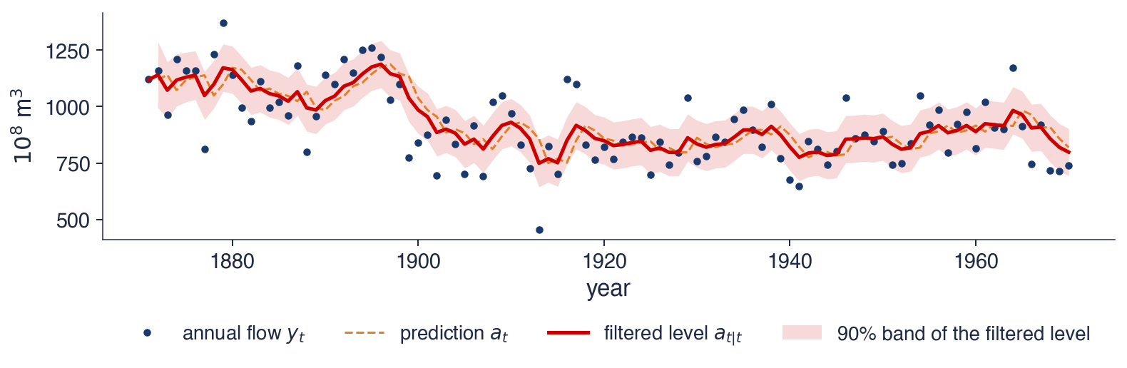


 TSA_ch10_state_space_examples