Bucharest University of Economic Studies IDA Institute Digital Assets Blockchain Research Center AI4EFin Artificial Intelligence for Energy Finance Romanian Academy, Institute for Economic Forecasting MSCA Digital Finance
“It is shown that common-stock prices, and the value of money can be regarded as an ensemble of decisions in statistical equilibrium, with properties quite analogous to an ensemble of particles in statistical mechanics.” — Osborne (1959)
It is shown that common-stock prices, and the value of money can be regarded as an ensemble of decisions in statistical equilibrium, with properties quite analogous to an ensemble of particles in statistical mechanics.
Osborne (1959) described the logarithms of stock prices with the tools of statistical physics: not prices but their logarithms behave like Brownian motion. The resulting model, geometric Brownian motion (GBM), is the price model behind the formula of Black & Scholes (1973). Prices are recorded daily or every few milliseconds, and continuous time gives one language for all these scales: Itô calculus, stochastic differential equations (SDEs) and the change of measure. The chapter's question is whether a single model can describe prices at any time scale.
The daily log returns of the S&P 500 (Standard & Poor's) since 1990 reject GBM in two respects. The excess kurtosis is 10.9 instead of 0, the worst day lies at −11.3 standard deviations, and 62 days lie beyond ±4 standard deviations, against 0.59 expected under the Normal distribution. The autocorrelation of absolute returns is 0.27 at lag 1 and still 0.14 at lag 50, so volatility comes in clusters (volatility clustering). Quadratic variation grows in steps: between September 2008 and March 2009, 1.6% of the days bring 15.2% of the quadratic variation of the whole sample. The drift cannot be pinned down from the data either: for a precision of ±1 percentage point, the S&P 500 would need 1,243 years of data and Bitcoin 17,028 years.
The chapter adds mean reversion, jumps (the Merton model) and stochastic volatility (the Heston model) in turn, then compares the estimated models with the data on 100 simulated samples of 9,245 days each. Merton reproduces the Hill tail statistic, 2.70 against 2.56 in the data, but not volatility clustering. Heston reproduces volatility clustering, with an autocorrelation of 0.28 at lag 1 against 0.27 in the data. No estimated model reaches the excess kurtosis of the data, 10.88: Merton gives 3.66 and Heston 3.21. The case studies show what one-factor models also miss: on SPY, the noise-robust non-linear least squares (NLLS) estimator gives a roughness exponent of −0.35, against 0 for Brownian motion.
The estimated models against the daily returns of the S&P 500: the autocorrelation of |r| at lags 1–50 (left), the excess kurtosis (middle) and the Hill statistic for the largest 5% of losses (right); for GBM, Merton and Heston the values are medians of 100 simulations, with 90% intervals. Interactive chart: “Which Model Reproduces the S&P 500? (1/2)” →
What you will be able to do
Derive solutions with Itô's lemma and simulate a stochastic differential equation with a known error order.
Compute GBM, Ornstein–Uhlenbeck, Merton and Heston estimates, with standard errors that respect what the sample identifies.
Interpret which feature of the data each model reproduces, and which feature none of them does.
Interpret why option pricing and interest-rate models use this language.
Geometric Brownian MotionGBM from Itô's lemma, maximum-likelihood estimation, the precision of the drift and the fit to the S&P 500.
Mean Reversion: the Ornstein–Uhlenbeck ProcessThe OU (Ornstein–Uhlenbeck, process) process, its exact discretisation as an AR(1), and the Vasicek and CIR (Cox–Ingersoll–Ross, model) models on the 3-month Treasury bill yield.
The chapter builds one language for prices observed at any frequency, in two parts:
The first part constructs Brownian motion as the limit of a rescaled random walk, develops Itô calculus from quadratic variation, and uses it to solve and simulate stochastic differential equations: geometric Brownian motion (GBM) for prices and the Ornstein–Uhlenbeck (OU) process for mean-reverting variables.
The second part asks which parameters the data identify, changes the probability measure to price claims, and adds jumps and stochastic volatility.
Each model is estimated on the same data and then compared with the S&P 500 on three yardsticks.
Prices are recorded at very different frequencies: daily closes for long histories, five-minute bars for recent years, and quotes every few milliseconds in electronic markets. A model formulated in continuous time has implications at every sampling interval at once, so a single set of parameters must explain daily returns, intraday returns and their aggregation. The question of the chapter is whether one model can do this.
The material is organised in two parts:
Part I covers Brownian motion, Itô calculus, simulation, GBM and mean reversion.
Part II covers the estimation of diffusions, the change of measure, jumps (the Merton model) and stochastic volatility (the Heston model), followed by the comparison of the estimated models with the data, two case studies and a section on research assisted by artificial intelligence (AI).
Option pricing, which uses the same tools, is the subject of Chapter 12.
In brief
What the models explain
Can one model describe prices at every time scale at once?
prices are recorded daily or every few milliseconds
Part I: Brownian motion, Itô calculus, simulation, geometric Brownian motion (GBM), mean reversion
Part II: estimating diffusions, change of measure, jumps, stochastic volatility
then models against data, two case studies, AI-assisted (Artificial Intelligence) discovery
What you should be able to do
derive solutions with Itô's lemma and simulate a stochastic differential equation with a known error order
compute GBM, Ornstein–Uhlenbeck, Merton and Heston estimates on data
with standard errors that respect what the sample identifies
interpret which feature of the data each model reproduces, and which feature none of them does
interpret why option pricing (Chapter 12) and interest-rate models use this language
Further Topics and Appendix: reading for familiarity
The empirical work uses three return series and two level series. The S&P 500 and the BET (Bucharest Exchange Trading), the benchmark index of the Bucharest Stock Exchange (BVB), are equity indices; Bitcoin trades seven days a week. The VIX, the Cboe Volatility Index computed by the Chicago Board Options Exchange (CBOE) from S&P 500 option prices, is used as a proxy for the variance in the Heston model. The short rate is the 3-month Treasury bill rate, series DTB3 of Federal Reserve Economic Data (FRED). Sample periods, numbers of observations and cleaning rules are in Further Topics and in the Appendix.
In brief
VIX: Cboe Volatility Index.
BET: Bucharest Exchange Trading (index).
BVB: Bursa de Valori București — the Bucharest Stock Exchange.
CBOE: Chicago Board Options Exchange.
FRED: Federal Reserve Economic Data.
DTB3: 3-Month Treasury Bill: secondary market rate (FRED series code).
Detailed examples and advanced topics are in Further Topics, after the Conclusions
the footer button leads there; the Back button returns to the starting slide
The chapter's question is therefore empirical as well as mathematical: each model is judged by the features of the data it reproduces at the frequencies observed. The construction starts with the simplest continuous-time object, Brownian motion.
From Random Walk to Brownian Motion
Brownian motion is the building block of every model in the chapter. This section obtains it as the limit of the random walk used for log prices in Chapter 2, and lists the properties that make it both tractable and unusual: Gaussian independent increments, the martingale property, self-similarity and paths that are continuous but nowhere differentiable.
From Random Walk to Brownian Motion: Donsker's Theorem (1/3)
Prices move in discrete steps, and the question is which process arises when the steps become smaller and more frequent. Start from the random walk \(S_0 = 0\),\(S_k = S_{k-1} + \xi_k = \xi_1 + \cdots + \xi_k\), where the steps \(\xi_i\) are independent and identically distributed (i.i.d.) with mean 0 and variance 1. In the log-price model of Chapter 2, \(\xi_k\) is the standardised return of day \(k\).
To pass to continuous time, put \(n\) steps in each unit of time and rescale:
\[W_n(t) = \frac{S_{\lfloor nt \rfloor}}{\sqrt{n}}, \qquad \operatorname{Var}\big(W_n(t)\big) = \frac{\lfloor nt \rfloor}{n} \to t,\]
(11.1)
where \(\lfloor nt \rfloor\) is the integer part of \(nt\). The factor \(\sqrt{n}\) is the only one that gives a non-degenerate limit: dividing by \(n\) would send the process to zero, and not dividing at all would make the variance explode. For each fixed \(t\), the central limit theorem (CLT) gives \(W_n(t) \to N(0, t)\).
Donsker's theorem is stronger: \(W_n \Rightarrow W\), where \(\Rightarrow\) denotes convergence in distribution of the whole path, not only of its value at each date (Billingsley, 1999). The limit \(W\) is Brownian motion, whatever the distribution of the steps. Functionals of the path, such as its maximum, therefore also converge to those of Brownian motion.
In brief
Question: which process do we get as price steps become smaller and more frequent?
The left chart shows three scaled random walks on \([0, 1]\), with \(n = 5\), 50 and 5,000 steps; the vertical axis is \(S_{\lfloor nt \rfloor}/\sqrt{n}\). The right chart shows, against \(n\) on a logarithmic axis, the probability that the maximum of \(W_n\) over \([0, 1]\) exceeds the level \(a\), estimated from simulated paths with a 95% confidence interval (CI). The horizontal line is the Brownian limit given by the reflection principle, \(P(\max_{t \le 1} W(t) > a) = 2\,(1 - \Phi(a))\), where \(\Phi\) is the standard Normal distribution function. The slider sets the level \(a\), and the ▶ button raises it step by step.
Question for the room For standard Brownian motion on [0, 1], raise the threshold from a = 1 to a = 2. What is the probability that the path maximum exceeds the new threshold?
Answer
About 0.0455. The reflection principle gives P(max W(t) > 2) = 2[1 − Φ(2)] ≈ 0.0455, against 0.3173 at a = 1. The value 0.0228 = 1 − Φ(2) concerns W(1) alone, not the maximum over the path. The value 0.1587 incorrectly halves the probability at threshold 1: the probability is not inversely proportional to the threshold. On the page, at a = 2, the random walk with n = 2,000 steps gives 0.042. The random-walk curves illustrate convergence to the Brownian benchmark; they do not sample the same Brownian path.
At \(a = 1\) the probability rises from 0.220 for \(n = 5\) to 0.316 for \(n = 2000\), towards the limit \(2(1 - \Phi(1)) = 0.3173\). A walk with few steps underestimates the maximum, because it does not see the values reached between its grid points.
As \(n\) grows, the step path becomes continuous and irregular, like a Brownian path. The probabilities in the right chart are estimated from 20,000 paths, and their convergence to the Brownian limit is slow, of order \(1/\sqrt{n}\).
The financial reading is direct. A coarse grid misses the maximum reached between observations, so daily closing prices understate the intraday range. Any statistic that depends on the extremes of the path, such as a barrier crossing or a drawdown, is biased when computed from sparse observations, and the bias shrinks only like \(1/\sqrt{n}\).
In brief
Left: three scaled random walks on \([0, 1]\) with \(n = 5\), \(50\) and \(5\,000\) steps
the vertical axis is \(S_{\lfloor nt \rfloor}/\sqrt{n}\)
for large \(n\) the step path becomes continuous and irregular, like a Brownian path
Right: \(P(\max_{t \le 1} W_n(t) > 1)\) against \(n\) on a log axis
estimated from 20 000 paths (95% CI)
the probability rises from \(0.220\) (\(n = 5\)) to \(0.316\) (\(n = 2000\))
the limit is the reflection-principle value \(2(1 - \Phi(1)) = 0.3173\)
\(\Phi\): standard Normal distribution function
A coarse grid misses the maximum reached between observations
A standard Brownian motion \((W_t)_{t \ge 0}\) is defined by four properties:
\(W_0 = 0\);
increments over disjoint intervals are independent;
\(W_t - W_s \sim N(0, t - s)\) for \(s < t\);
the paths are continuous.
Its existence was established by Wiener (1923). On a grid it is simulated exactly by \(W_{t + \Delta t} = W_t + \sqrt{\Delta t}\,Z\), with \(Z \sim N(0, 1)\).
Several properties follow from the definition. Brownian motion is a Gaussian process with \(\operatorname{Cov}(W_s, W_t) = \min(s, t)\). It is a martingale: \(\mathbb{E}[W_t \mid \mathcal{F}_s] = W_s\), where \(\mathcal{F}_s\) is the information available at \(s\); this is the continuous-time version of the efficient-market random walk of Chapter 2. It is self-similar: for any \(c > 0\), the rescaled process \(\{c^{-1/2} W_{ct}\}\) is again a standard Brownian motion, so a zoomed piece of a path has the same law as the whole path.
The last property is the one that changes the calculus. The paths are continuous but nowhere differentiable: the difference quotient \((W_{t+h} - W_t)/h\) has standard deviation \(1/\sqrt{h}\), which tends to infinity as \(h \to 0\). Ordinary calculus, which relies on derivatives, does not apply to Brownian paths. Paths and their scaling are illustrated in Further Topics.
In brief
Standard Brownian motion: four defining properties
Donsker's theorem justifies Brownian motion as the limit of any random walk with finite-variance steps. Its paths are continuous but too irregular for ordinary calculus; the next section measures this irregularity and builds the calculus that replaces it.
Quadratic Variation and Itô Calculus
A Brownian path has infinite length but a finite and deterministic sum of squared increments. This section defines the two notions of variation, measures them on simulations and on the S&P 500, and uses quadratic variation to build the Itô integral and Itô's lemma, the chain rule of stochastic calculus.
Why does ordinary calculus fail on a Brownian path, and what replaces it? Take a grid \(0 = t_0 < \cdots < t_n = T\) with step \(\Delta t = T/n\) and increments \(\Delta W_k = W_{t_k} - W_{t_{k-1}}\). The total variation\(\sum_k |\Delta W_k|\), the length of the path measured on the grid, has mean \(\sqrt{2nT/\pi}\), which tends to infinity: a Brownian path has infinite length.
where \(Q_n = \sum_{k=1}^{n} (\Delta W_k)^2\). In (11.2) a sum of random terms has a deterministic limit, because its variance vanishes as the grid becomes finer. With one year of daily data the relative error of \(Q_n\) is \(\sqrt{2/252}\), about 9%. This is the idea behind realised variance in Chapter 9.
Itô calculus summarises (11.2) in the shorthand \((\mathrm{d}W_t)^2 = \mathrm{d}t\): over a short interval the squared increment is not negligible relative to the length of the interval, as it would be for a differentiable path, but equal to it in the limit.
In brief
Question: why does ordinary calculus fail on a Brownian path, and what replaces it?
The left chart follows one Brownian path on \([0, 1]\) observed on grids from 16 to 65,536 intervals and shows the sum \(\sum_k |\Delta W_k|^p\) against the number of intervals. The slider sets the exponent \(p\):\(p = 1\) gives the total variation and \(p = 2\) the quadratic variation; the ▶ button moves \(p\) from 0.5 to 3. The right chart shows the cumulative sum of squared daily log returns of the S&P 500, \(\sum r_t^2\), together with the straight line \(\sigma^2 t\) that GBM would produce; the selector highlights one of two crisis periods.
Question for the room For standard Brownian motion on [0, 1], set p = 1.5. If the number of equal intervals increases fourfold, by what factor does the mean of Σ|ΔW|^1.5 change?
Answer
By √2 ≈ 1.41. The mean is n^(1 − p/2)·E|Z|^p, where Z has the standard Normal distribution; for p = 1.5, the factor is 4^0.25 = √2. A factor of 4 ignores the shrinking increments; 1/√2 reverses the direction of the change. This relation concerns the mean, not an exact equality for every path: on the path of the page, the sum goes from 9.75 with 16,384 intervals to 13.83 with 65,536 intervals (ratio 1.42). Only the exponent 2 gives a non-degenerate limit: Σ(ΔW)² tends to T = 1 (1.006 on the finest grid), hence (dW)² = dt.
For \(p = 2\) the sum settles at 1.006 on the finest grid, close to \(T = 1\), whereas for \(p = 1\) it keeps growing: 205 on the finest grid, against \(\sqrt{2n/\pi} = 204\). Only the exponent 2 gives a limit that is neither zero nor infinite.
On the S&P 500, the cumulative sum of squared daily log returns reaches 1.188 over 36.7 years, which corresponds to an average annual volatility of 18.0%. Under GBM, with constant volatility \(\sigma\), the quadratic variation grows along the straight line \(\sigma^2 t\).
The data do not follow the line: the sum rises in steps. Between September 2008 and March 2009, 1.6% of the days bring 15.2% of the quadratic variation of the whole sample; between February and April 2020, 0.5% of the days bring 7.8%. Volatility is therefore itself random. The Heston model of Section 10 gives it its own dynamics.
In brief
Left: one Brownian path on grids with 16 to 65,536 intervals
the quadratic variation settles at \(1.006\) (\(T = 1\))
the total variation keeps growing: \(205\) against \(\sqrt{2n/\pi} = 204\)
Right: cumulative \(\sum r_t^2\) of the S&P 500, \(1.188\) over 36.7 years
average volatility \(18.0\%\)
under geometric Brownian motion it would follow the straight line \(\sigma^2 t\)
The sum rises in steps
September 2008 – March 2009: \(1.6\%\) of the days, but \(15.2\%\) of the quadratic variation
February – April 2020: \(0.5\%\) of the days, but \(7.8\%\) of the quadratic variation
The gain from holding \(H_t\) units of an asset whose price moves like \(W\) is \(\int_0^T H_t\,\mathrm{d}W_t\). The integral cannot be defined path by path as a Riemann–Stieltjes integral, because the total variation of \(W\) is infinite. The Itô integral defines it as a limit in mean square of sums in which the integrand is evaluated at the left end point of each interval:
The integrand must be adapted, that is, \(H_t\) uses only the information available up to \(t\), and must satisfy \(\mathbb{E}\big[\int_0^T H_t^2\,\mathrm{d}t\big] < \infty\). The left end point has a financial meaning: the position over \([t_{k-1}, t_k]\) is chosen before the next price move is known.
In brief
Goal: a meaning for \(\int_0^T H_t\,\dd W_t\)
the gain of holding \(H_t\) units of an asset priced \(W\)
Riemann–Stieltjes integration fails because the total variation is infinite
Itô integral: the limit in mean square of sums with the integrand at the left end point
Moreover, \(t \mapsto \int_0^t H_s\,\mathrm{d}W_s\) is a martingale: no trading strategy in a driftless asset earns money on average. Under weaker integrability conditions the integral is only a local martingale; the details are in the Appendix.
The choice of the evaluation point matters. The Stratonovich integral evaluates the integrand at the average of the end points, \(\tfrac12(H_{t_{k-1}} + H_{t_k})\), and gives a different number, because the extra term picks up the quadratic variation. Finance uses the Itô integral, since a position evaluated at the right end point would use the price at \(t_k\) before it is known. A worked example, \(\int_0^T W_t\,\mathrm{d}W_t\), is in Further Topics.
In brief
Zero mean: \(\E\left[\int_0^T H_t\,\dd W_t\right] = 0\)
An Itô process is written \(\mathrm{d}X_t = a_t\,\mathrm{d}t + b_t\,\mathrm{d}W_t\), shorthand for \(X_t = X_0 + \int_0^t a_s\,\mathrm{d}s + \int_0^t b_s\,\mathrm{d}W_s\), with an adapted drift \(a_t\) and an adapted diffusion coefficient \(b_t\). For a function \(f(t, x)\) that is continuously differentiable once in \(t\) and twice in \(x\),Itô's lemma (Itô, 1944) gives
where \(f_t = \partial f/\partial t\),\(f_x = \partial f/\partial x\) and \(f_{xx} = \partial^2 f/\partial x^2\) are evaluated at \((t, X_t)\).
The lemma follows from a Taylor expansion to second order, with the multiplication rules \(\mathrm{d}t \cdot \mathrm{d}t = 0\),\(\mathrm{d}t \cdot \mathrm{d}W = 0\) and \(\mathrm{d}W \cdot \mathrm{d}W = \mathrm{d}t\). In ordinary calculus the second-order term disappears; here \((\mathrm{d}X_t)^2 = b_t^2\,\mathrm{d}t\) by (11.2), so the term \(\tfrac{1}{2} b_t^2 f_{xx}\,\mathrm{d}t\) remains. This term is the whole difference from the ordinary chain rule, and it reappears in every model of the chapter. The multivariate version, with quadratic covariation, is in Further Topics.
In brief
Itô process: \(\dd X_t = a_t\,\dd t + b_t\,\dd W_t\)
drift \(a_t\), diffusion coefficient \(b_t\), both adapted
shorthand for \(X_t = X_0 + \int_0^t a_s\,\dd s + \int_0^t b_s\,\dd W_s\)
Itô's lemma: for \(f(t, x)\) continuously differentiable once in \(t\) and twice in \(x\)Itô (1944)
Quadratic variation, \((\mathrm{d}W)^2 = \mathrm{d}t\), is the fact on which the rest of the chapter rests: it defines the Itô integral, adds the second-order term to the chain rule, and in the data shows that volatility is not constant.
Stochastic Differential Equations and Simulation
Most models of the chapter are stochastic differential equations (SDEs) whose drift and diffusion depend on the current state. Some have exact solutions, others must be simulated on a grid. This section introduces the two standard schemes and the measure of their accuracy along paths.
Stochastic Differential Equations and the Euler–Maruyama Scheme
GBM, the Ornstein–Uhlenbeck process and the Merton model have exact transition distributions, so they can be simulated on any grid with no discretisation error. The Heston model has a closed-form characteristic function but no elementary transition that is easy to simulate; exact simulation exists Broadie & Kaya (2006) but is costly. Conditions for existence and uniqueness of solutions are in the Appendix.
The simplest approximation, the Euler–Maruyama scheme (Higham, 2001), freezes the coefficients over each step:
where \(X_k\) is the approximation at \(t_k = k\Delta t\) and the \(Z_k\) are i.i.d. \(N(0, 1)\). The question is how large the resulting discretisation error is.
In brief
Question: how do we simulate a model whose transition (the law of \(X_{t+\Delta t}\) given \(X_t\)) is not easy to simulate, such as Heston?
with \(b' = \mathrm{d}b/\mathrm{d}x\). The correction has conditional mean zero, because \(\mathbb{E}[(\Delta W_k)^2] = \Delta t\), so it does not change the expected value of the step; it improves the accuracy of each path.
Path accuracy is measured by the strong error, \(\mathbb{E}|X_T - X_T^{\Delta t}| \le C\,\Delta t^{\gamma}\), where \(X_T\) is the exact solution, \(X_T^{\Delta t}\) the scheme with step \(\Delta t\),\(C\) a constant and \(\gamma\) the strong order. Euler–Maruyama has \(\gamma = 1/2\) and Milstein \(\gamma = 1\). The strong order matters for path-dependent quantities, such as hedging errors and barrier crossings. Expected values of functions of \(X_T\) depend on the weak order instead, which is discussed with a numerical comparison of the two schemes in Further Topics.
Models with exact transitions are simulated without error; the others are simulated with Euler–Maruyama or Milstein, whose error along paths shrinks like \(\Delta t^{1/2}\) and \(\Delta t\) respectively. The first model to which Itô's lemma is applied is the price model of the next section.
Geometric Brownian Motion
Geometric Brownian motion is the reference model for prices: it keeps prices positive and gives returns whose distribution does not depend on the price level. This section solves it with Itô's lemma, estimates it by maximum likelihood, shows how imprecisely the drift is identified, and tests its implications on the S&P 500.
Geometric Brownian Motion (GBM) from Itô's Lemma (1/2)
A price model should keep prices positive and give percentage returns with the same distribution at every price level. GBM, proposed by Osborne (1959) and Samuelson (1965) and used by Black & Scholes (1973), satisfies
By (11.10) the log price grows at the log drift \(m = \mu - \sigma^2/2\), not at \(\mu\). The difference comes from the second-order term of Itô's lemma, and its economic meaning is that volatility lowers the growth of the median investor's wealth. With \(\sigma = 18\%\) the cost is \(\sigma^2/2 = 1.6\) percentage points a year; with \(\sigma = 67\%\), the volatility of Bitcoin, it reaches 22 percentage points a year.
GBM has sharp testable implications. The log returns \(r_t = \ln(S_t/S_{t - \Delta t})\) are i.i.d. \(N(m\Delta t, \sigma^2\Delta t)\) at every frequency. Hence skewness and excess kurtosis are zero, there is no autocorrelation in \(r_t\),\(|r_t|\) or \(r_t^2\), and the variance is proportional to the horizon. The rest of the section estimates the model and checks these implications. The distribution of future prices under GBM is illustrated in Further Topics.
In brief
The log price grows at the log drift \(m = \mu - \sigma^2/2\), not at \(\mu\)
volatility lowers the growth of the median investor's wealth
With \(\sigma = 18\%\), the cost is \(\sigma^2/2 = 1.6\) percentage points a year
With \(\sigma = 67\%\) (Bitcoin), the cost reaches 22 percentage points a year
Testable implications: \(r_t = \ln(S_t/S_{t - \Delta t})\) i.i.d. \(N(m\Delta t, \sigma^2\Delta t)\) at every frequency
Skewness and excess kurtosis are zero
There is no autocorrelation in \(r_t\), \(|r_t|\) or \(r_t^2\)
where \(\bar r\) is the mean log return. Under GBM the two estimators have very different precision:
\[\mathrm{SE}(\hat\sigma) = \frac{\sigma}{\sqrt{2n}}, \qquad \mathrm{SE}(\hat m) = \frac{\sigma}{\sqrt{T}}.\]
(11.11)
The standard error (SE) of \(\hat\sigma\) shrinks with the number of observations, whereas the SE of \(\hat m\) depends only on the calendar span\(T\). The reason is that \(\sum_t r_t = \ln(S_T/S_0)\): the estimator of the drift uses only the first and the last price, however many prices lie between them.
The table confirms the asymmetry on the three markets. The SE is 0.1–0.7 percentage points for volatility but 3–19 percentage points for the log drift. For the S&P 500 over 36.7 years, \(\hat\sigma = 18.0\%\) with SE 0.13 and \(\hat m = 8.3\%\) with SE 3.0, so \(\hat\mu = 8.3\% + 1.62\% = 10.0\%\) a year. For Bitcoin, over 12.0 years, the log drift of 43.1% has an SE of 19.2 percentage points.
In brief
Maximum likelihood estimation (MLE) from \(n\) log returns at step \(\Delta t\), over \(T = n\Delta t\) years
\(\hat\sigma^2 = \frac{1}{n\Delta t}\sum_t (r_t - \bar r)^2\), \(\hat m = \bar r / \Delta t\), \(\hat\mu = \hat m + \hat\sigma^2/2\) (\(\bar r\): mean log return)
under GBM, the standard error (SE) \(\mathrm{SE}(\hat\sigma) = \sigma/\sqrt{2n}\) shrinks with the number of observations
\(\mathrm{SE}(\hat m) = \sigma/\sqrt{T}\) depends only on the calendar span
reason: \(\sum_t r_t = \ln(S_T/S_0)\) uses only the first and the last price
Years
\(\hat\sigma\) (%)
\(\mathrm{SE}(\hat\sigma)\)
\(\hat m\) (%)
\(\mathrm{SE}(\hat m)\)
S&P 500
\(36.7\)
\(18.0\)
\(0.13\)
\(8.3\)
\(3.0\)
BET
\(26.5\)
\(22.2\)
\(0.19\)
\(16.1\)
\(4.3\)
Bitcoin
\(12.0\)
\(66.6\)
\(0.71\)
\(43.1\)
\(19.2\)
The SE is 0.1–0.7 percentage points for volatility, but 3–19 points for the log drift
S&P 500: \(\hat\mu = 8.3\% + 1.62\% = 10.0\%\) per year
The standard errors in (11.11) are conditional on GBM. If returns are independent but have excess kurtosis \(k\), the SE of \(\hat\sigma\) is inflated by \(\sqrt{(k + 2)/2}\), which is 2.5 for the S&P 500. A block bootstrap gives SEs that also allow for dependence (Seminar 11, B1).
The two SEs also need different moment conditions. The drift SE requires only a finite variance. The volatility SE requires a finite fourth moment, which Chapter 1 questions for daily returns.
In brief
These SE are conditional on GBM
with excess kurtosis \(k\), even independent returns inflate \(\mathrm{SE}(\hat\sigma)\) by \(\sqrt{(k + 2)/2} = 2.5\) (S&P 500)
The left chart shows the half-width of the 95% CI for the log drift, \(1.96\,\hat\sigma/\sqrt{T}\), against the years of data, for each market; p.p. means percentage points. The right chart estimates the log drift and the volatility of the S&P 500 on rolling windows, with their 95% CIs; the slider sets the window length from 1 to 20 years, and the ▶ button lengthens it year by year.
Question for the room Compare two GBM models with constant parameters: the first has σ = 20% and 10 years of data; the second has σ = 40% and 40 years of data. How does the half-width of the 95% interval for the log drift change from the first to the second?
Answer
It stays the same. The half-width is 1.96σ/√T: approximately 12.4 percentage points in both cases. Doubling volatility exactly offsets the halving of 1/√T. ‘It halves’ ignores the volatility change; ‘it doubles’ ignores the observation span. For the S&P 500 (σ = 18%), 10 years of data give ±11.2 percentage points, however fine the grid: the 2,520 daily returns do not reduce this half-width. On 10-year windows the log drift ranges from −6.0% (2009-03) to 15.8% (2000-09); with this precision the swings cannot be safely attributed to changes in the drift.
With 10-year windows, the log drift ranges from −6.0% (window ending in March 2009) to 15.8% (September 2000), and each estimate has a CI of about ±11 percentage points. The volatility stays between 14.1% and 22.3%.
Inverting (11.11) gives the span needed for a given precision. A 95% CI of ±1 percentage point requires \((1.96\,\hat\sigma/0.01)^2\) years of data: 1,243 years for the S&P 500 and 17,028 years for Bitcoin. Sampling more often does not help, because the precision depends on \(T\) alone.
The rolling estimates make the same point. With a CI of about ±11 percentage points, the swings of the 10-year drift from −6.0% to 15.8% cannot be safely attributed to changes in the true drift. The volatility, between 14.1% and 22.3%, is estimated precisely, but it is visibly not constant.
Option pricing in Chapter 12 avoids this difficulty: under the risk-neutral measure only \(\sigma\) enters the price, as the Girsanov theorem of Section 8 shows.
In brief
Left: half-width of the 95% CI for the drift against years of data
A precision of \(\pm 1\) point needs \((1.96\,\hat\sigma/0.01)^2\) years of data
S&P 500: \((1.96\,\hat\sigma/0.01)^2 = 1\,243\) years
17 028 years for Bitcoin
Right: S&P 500 on rolling 10-year windows
the log drift ranges from \(-6.0\%\) (window ending 2009-03) to \(15.8\%\) (2000-09)
each estimate has a CI of about \(\pm 11\) points
with this precision, the swings cannot be safely attributed to changes in the drift
volatility stays between \(14.1\%\) and \(22.3\%\): precise, but not constant
The left chart is a quantile–quantile (QQ) plot of the standardised daily log returns of the S&P 500 against the Normal distribution; points off the diagonal are quantiles that the Normal distribution does not match. The slider sets a threshold \(k\), in standard deviations, and the readout counts the days beyond \(\pm k\) against the number expected under the Normal distribution. The right chart shows the autocorrelation function (ACF) of the series chosen with the selector, \(|r_t|\),\(r_t^2\) or \(r_t\), with the 95% band of 200 GBM samples of the same length.
Question for the room How many days beyond ±4 standard deviations should appear in 9,245 days if returns had the Normal distribution?
Answer
About 0.59 = 9,245 · 2(1 − Φ(4)), counting both tails; one tail would give 0.29. The data have 62, and the worst day lies at −11.3 standard deviations; the excess kurtosis is 10.9. The ACF of |r| is 0.27 at lag 1 and 0.14 at lag 50, while the GBM band stays below 0.024.
At \(k = 4\), 62 days lie beyond ±4 standard deviations, against 0.59 expected under the Normal distribution. The ACF of \(|r_t|\) is 0.27 at lag 1 and still 0.14 at lag 50, while the GBM band stays below 0.024 in absolute value.
The data reject the first implication of GBM, Normal returns. The excess kurtosis is 10.9 instead of 0, the worst day lies at −11.3 standard deviations, and the Jarque–Bera (JB) statistic, which tests zero skewness and zero excess kurtosis jointly, is 45,805 against a 5% critical value of 5.99 from the \(\chi^2_2\) distribution. The kurtosis figure needs care: the sample kurtosis consistently estimates a finite kurtosis only if the fourth moment is finite, which Chapter 1 questions, and inference on it usually requires a finite eighth moment.
The data also reject the second implication, independence. Absolute returns are autocorrelated over at least 50 days, far outside the band produced by GBM. GBM thus fails on both stylised facts of Chapter 1(Cont, 2001): fat tails and volatility clustering.
The result is descriptive: the data reject two implications of GBM without identifying the mechanism that produces them. The rest of the chapter adds mean reversion, jumps and random volatility, and asks which of them reproduces which feature. The formulas of this section are collected in a recap.
In brief
Left: quantile–quantile (QQ) plot of standardised daily log returns against the Normal distribution
excess kurtosis \(10.9\) instead of 0
the sample kurtosis consistently estimates a finite kurtosis only with a finite fourth moment, which Chapter 1 questions
inference on the kurtosis usually requires a finite eighth moment
worst day at \(-11.3\) standard deviations
62 days beyond \(\pm 4\) standard deviations, against \(0.59\) expected under the Normal distribution
Jarque–Bera (JB) statistic: 45 805 against the 5% critical value 5.99 (\(\chi^2_2\))
JB tests zero skewness and zero excess kurtosis jointly
Right: autocorrelation function (ACF) of \(|r_t|\)
\(0.27\) at lag 1 and still \(0.14\) at lag 50
the 95% band from 200 GBM samples of the same length stays below \(0.024\) in absolute value
GBM fails on both stylised facts (fat tails, volatility clustering) of Chapter 1Cont (2001)
the rest of the chapter adds mean reversion, jumps and random volatility
Type of evidence: description (it shows what happened in the data, without testing a cause)
the data reject two implications of GBM without identifying the mechanism that produces them
GBM gives positive prices and an exact solution, its volatility is estimated precisely, but its drift is identified only over centuries. On the S&P 500 it fails twice: the tails are far heavier than Normal, and absolute returns are persistent. The next section turns to variables that do not drift away but return to a normal level.
Mean Reversion: the Ornstein–Uhlenbeck Process
Interest rates, volatility indices and spreads do not drift away like stock prices; they are pulled back towards a normal level. The Ornstein–Uhlenbeck process is the simplest diffusion with this property. This section defines it, shows that its discrete samples follow an autoregression of order 1, introduces the two classical short-rate models built on it, and estimates the Vasicek model on the 3-month Treasury bill rate.
where \(\theta\) is the long-run mean, \(\kappa\) the speed of mean reversion and \(\sigma\) the volatility. Above \(\theta\) the drift is negative, below \(\theta\) it is positive: the drift acts as a force that pulls \(x\) back to \(\theta\), with a strength proportional to the distance. The process is used for interest rates (Vasicek, 1977), volatility, spreads and commodity prices.
The speed is usually reported as a half-life, \(\ln 2/\kappa\), the time needed for the expected deviation from \(\theta\) to halve. With \(\kappa = 0.5\) per year the half-life is 1.39 years. The solution of (11.12), obtained with Itô's lemma in three steps, is derived in Further Topics: \(x_t\) is Normal, with a conditional mean that decays exponentially towards \(\theta\) and a variance that converges to \(\sigma^2/(2\kappa)\).
In brief
Question: how do we model a variable that returns to a normal level?
Sampled at step \(\Delta t\), the OU process is exactly an autoregressive model of order 1, AR(1):
\[\begin{gathered} x_{t+\Delta t} = a + b\,x_t + \varepsilon_t, \\ b = e^{-\kappa\Delta t}, \quad a = \theta(1 - b), \quad \operatorname{Var}(\varepsilon_t) = \frac{\sigma^2}{2\kappa}\,(1 - b^2). \end{gathered}\]
(11.13)
The errors \(\varepsilon_t\) are i.i.d. Normal, so the maximum-likelihood estimator coincides with ordinary least squares (OLS) of \(x_{t + \Delta t}\) on \(x_t\). OLS gives the intercept \(\hat a\), the slope \(\hat b\) and the residual standard deviation \(\hat s_\varepsilon\), and the mapping (11.13) is inverted: \(\hat\kappa = -\ln\hat b/\Delta t\),\(\hat\theta = \hat a/(1 - \hat b)\) and \(\hat\sigma = \hat s_\varepsilon\sqrt{2\hat\kappa/(1 - \hat b^2)}\).
Standard errors of \(\hat\kappa\) and \(\hat\theta\) follow from the delta method applied to the OLS covariance of \((\hat a, \hat b)\). Because \(\hat\kappa\) depends on \(\hat b\) only, with \(\partial\kappa/\partial b = -1/(b\Delta t)\), the variance of \(\hat b\) suffices (Seminar 11, A1).
With daily data, \(b = e^{-\kappa\Delta t}\) is very close to 1, so the regression is close to a unit root. The speed \(\kappa\) is then estimated imprecisely, for the same reason that unit-root tests have low power. Three speeds of reversion are compared on simulated paths in Further Topics.
In brief
Sampled at step \(\Delta t\), the Ornstein–Uhlenbeck (OU) process is exactly an autoregressive model of order 1 (AR(1))
Standard errors of \(\hat\kappa\) and \(\hat\theta\): the delta method (linearising the transformation), from the OLS covariance of \((\hat a, \hat b)\)
\(\hat\kappa\) depends on \(\hat b\) only: \(\partial\kappa/\partial b = -1/(b\Delta t)\)
In the Vasicek model (Vasicek, 1977) the short rate \(r_t\) is an OU process. Its distribution is Normal, so negative rates have positive probability; in the long run this probability is \(\Phi(-\theta\sqrt{2\kappa}/\sigma)\). In exchange, bond prices and yields have closed forms, derived with the Feynman–Kac formula in Section 8.
Volatility shrinks as the rate approaches zero, and the rate stays strictly positive if \(2\kappa\theta \ge \sigma^2\), the Feller condition (Feller, 1951).
The left chart shows the daily 3-month US (United States) Treasury bill rate (DTB3) together with the estimated Vasicek long-run mean \(\hat\theta\) and a band of \(\hat\theta\) plus or minus two stationary standard deviations (s.d.). The right chart shows the estimate of \(\kappa\) with its 95% CI over subperiods. The two sliders set the start and the end of the estimation sample, and the ▶ button extends the end year by year.
Question for the room Does a positive κ̂ over 1954–2026 show that the short rate is mean-reverting?
Answer
No. κ̂ = 0.101 (SE 0.051) means a half-life of 6.8 years, and the daily AR(1) coefficient is 0.99960, almost a unit root. Over subperiods κ̂ is −0.034, 0.213 and 0.032, and two of the three intervals include zero. The asymptotic interval over 1954–2026 barely excludes zero (0.101 − 1.96 · 0.051 = 0.001), but near a unit root the distribution of κ̂ is not Normal and is biased upwards; the bootstrap test of the random-walk null gives a p-value of 0.287.
On the full sample, 1954–2026, \(\hat\theta = 4.55\%\),\(\hat\kappa = 0.101\) (SE 0.051), a half-life of 6.8 years, and \(\hat\sigma = 1.33\%\). The daily AR(1) coefficient is \(\hat b = 0.99960\), almost a unit root.
The estimates depend strongly on the period. Over three subperiods \(\hat\kappa\) is −0.034 in 1954–1979, a negative and therefore explosive value, 0.213 in 1980–2007 and 0.032 in 2008–2026, and two of the three CIs include zero.
The asymptotic CI is not a reliable guide here. Under the random-walk null \(\kappa = 0\), the distribution of \(\hat\kappa\) is not Normal and is shifted upwards. The test is therefore done by parametric bootstrap, with 500 random walks of the same length as the data. The p-value is 0.287: we do not reject the random walk, so the sample does not establish mean reversion (Seminar 11, B2).
The result is descriptive. The upward bias of \(\hat\kappa\) in persistent samples is quantified in Further Topics, together with an OU fit to the VIX.
In brief
Left: daily 3-month United States (US) Treasury bill rate (DTB3), 1954–2026
with the Vasicek long-run mean \(\hat\theta = 4.55\%\)
band: \(\hat\theta\) plus/minus two stationary standard deviations (s.d.)
\(\hat\kappa = 0.101\) (SE \(0.051\)), a half-life of \(6.8\) years
volatility \(\hat\sigma = 1.33\%\)
Daily AR(1) coefficient \(\hat b = 0.99960\): almost a unit root
Right: \(\hat\kappa\) with 95% CI over three periods
\(-0.034\) in 1954–1979 (explosive), \(0.213\) in 1980–2007 and \(0.032\) in 2008–2026
Two of the three CIs include zero
Test of the random-walk null (\(\kappa = 0\)): parametric bootstrap
500 random walks of the same length
reason: under \(\kappa = 0\) the distribution of \(\hat\kappa\) is not Normal and is shifted upwards
p-value \(= 0.287\): the sample does not establish mean reversion (Seminar 11, B2)
The OU process gives exact Normal transitions and an AR(1) for discrete samples, so its estimation reduces to a regression. On the Treasury bill rate the estimated speed is small, unstable across periods and not significantly different from zero by bootstrap. Why the speed is so hard to estimate is the subject of the next section.
Estimating Diffusions: Identification of Drift and Volatility
The estimates so far share a pattern: volatility is precise, while the drift of GBM and the speed of the OU process are not. This section explains the pattern with two asymptotic schemes:
Infill asymptotics refines the grid on a fixed span.
Long-span asymptotics lengthens the span.
Each identifies a different set of parameters.
Infill Asymptotics: Effect of the Sampling Frequency
Which parameters do we learn from sampling more often, and which only from more years? Under infill asymptotics the step \(\Delta\) tends to zero on a fixed interval \([0, T]\). For an Itô process the realised quadratic variation converges:
The quadratic variation, and hence, under regularity conditions, \(b_t^2\) along the path, is identified without error in the limit. This requires that the quadratic variation be observable: a continuous Itô process measured without noise. Recovering the whole diffusion function \(b(x)\), or the parameters of a given specification, needs further conditions.
Sampling more often therefore helps the volatility \(\sigma\) of GBM (Section 5) and the diffusion function \(b(x)\) of a general model, which can be estimated nonparametrically (Further Topics).
In brief
Question: which parameters do we learn from sampling more often, and which only from more years?
The drift is not consistently estimable on a fixed span. The Fisher information \(I(m) = -\mathbb{E}[\partial^2\ell/\partial m^2]\), where \(\ell\) is the log-likelihood, bounds the variance of any unbiased estimator, \(\operatorname{Var}(\hat m) \ge 1/I(m)\). For \(n\) GBM returns,
so the information grows with the span \(T\), not with the number of observations \(n\).
The OU speed behaves in the same way. Its asymptotic variance is \(\operatorname{Var}(\hat\kappa) \approx (e^{2\kappa\Delta} - 1)/(T\Delta)\), which tends to \(2\kappa/T\) as \(\Delta \to 0\) (derivation in Seminar 11, A1). The bias of \(\hat\kappa\) does not shrink with finer sampling either (Yu, 2012): as \(\Delta \to 0\),\(b = e^{-\kappa\Delta} \to 1\), and \(\hat\kappa\) is far from Normal whenever \(\kappa T\) is small.
The imprecise GBM drift and the biased \(\hat\kappa\) thus have the same cause. Likelihood methods for nonlinear diffusions and the comparison of Vasicek, CIR and CKLS (Chan–Karolyi–Longstaff–Sanders) on the Treasury bill rate are in Further Topics.
In brief
Long span: \(T \to \infty\)
The drift is not consistently estimable on a fixed span
Fisher information \(I(m) = -\E[\partial^2\ell/\partial m^2]\) (\(\ell\): log-likelihood) bounds \(\Var(\hat m) \ge 1/I(m)\)
for \(n\) GBM returns \(I(m) = n\Delta t/\sigma^2 = T/\sigma^2\)
Frequent sampling identifies the diffusion coefficient; drift and mean-reversion speed are identified only by the length of the sample. A model estimated on a few decades of data gives precise volatilities and imprecise drifts, whatever the frequency. For pricing, the next section shows that the drift is not needed.
Change of Measure: Girsanov and Feynman–Kac
Prices of traded claims are not computed with the real-world probabilities. This section shows why on a one-period example, states Girsanov's theorem, which builds the pricing measure in continuous time, interprets the change of drift as the market price of risk, and derives the pricing equation with the Feynman–Kac formula.
Why Prices Use a Different Probability: a One-Period Example (1/2)
A stock costs 100 today and tomorrow is worth either 120 (up) or 90 (down). The interest rate is 0, and the real-world probability of the up state is \(p = 0.6\). A claim pays 1 in the up state and 0 in the down state.
The claim can be replicated with \(\Delta\) shares and \(B\) in cash. The conditions \(120\Delta + B = 1\) and \(90\Delta + B = 0\) give \(\Delta = 1/30\) and \(B = -3\), so the replicating portfolio costs \(100/30 - 3 = 1/3\). Any other price for the claim would allow an arbitrage: buy the cheaper of the claim and its replica and sell the other.
The same price is an expectation, but not under \(p\). The weight \(q = (100 - 90)/(120 - 90) = 1/3\) is the only one with \(120q + 90(1 - q) = 100\), that is, the only probability under which the stock is priced at its expected value, and the claim's price is \(q \cdot 1 = 1/3\). The real-world probability \(p\) never enters.
In brief
A stock costs 100 today and tomorrow is worth 120 (up) or 90 (down)
the interest rate is 0
the real-world probability of up is \(p = 0.6\)
A claim pays 1 if up and 0 if down
replicate it with \(\Delta\) shares and \(B\) in cash
\(120\Delta + B = 1\) and \(90\Delta + B = 0\) give \(\Delta = 1/30\), \(B = -3\)
the replica costs \(1/3\), and any other price is an arbitrage
The same price is the expectation under \(q = (100 - 90)/(120 - 90) = 1/3\)
\(q\) is the only weight with \(120q + 90(1 - q) = 100\)
\(p\) never enters
Why Prices Use a Different Probability: a One-Period Example (2/2)
The example generalises. Absence of arbitrage means that discounted prices of traded assets are martingales under a probability measure \(Q\) equivalent to the real-world measure \(P\): this is the fundamental theorem of asset pricing (Chapter 5 of Shreve (2004)). In continuous time, Girsanov's theorem builds \(Q\).
The checks on the slide test the logic. If \(p = 0.9\), the price of the claim is still 1/3, because \(p\) does not enter. If the down state is 80 instead of 90, then \(q = 20/40 = 1/2\) and the price becomes 1/2: the pricing weights depend on the possible outcomes, not on how likely they are.
In brief
In general, absence of arbitrage means that discounted traded prices are martingales under an equivalent measure \(Q\)
fundamental theorem of asset pricing, Shreve (2004), Ch. 5
Girsanov builds \(Q\) in continuous time
Check: what is the price of the claim if \(p = 0.9\)?
Two measures are equivalent if they assign probability zero to the same events. An equivalent measure \(Q\) is defined from \(P\) through the Radon–Nikodym density
with \(\theta_s\) adapted. Since \(Z_T > 0\) and \(\mathbb{E}^P[Z_T] = 1\), the density reweights the probability of each path: \(Q(A) = \mathbb{E}^P[Z_T\,\mathbf{1}_A]\).
Girsanov (1960) shows that under \(Q\) the process \(\tilde W_t = W_t + \int_0^t \theta_s\,\mathrm{d}s\) is a Brownian motion. A sufficient condition is the Novikov condition, \(\mathbb{E}\big[e^{\frac{1}{2}\int_0^T \theta_s^2\,\mathrm{d}s}\big] < \infty\). Below, \(\theta_s\) will be the market price of risk.
In brief
Real-world measure \(P\) and an equivalent measure \(Q\), linked by the Radon–Nikodym density
For continuous Itô processes only the drift changes. The diffusion coefficient, and with it the quadratic variation, is the same under \(P\) and \(Q\), which is why volatility estimated from historical data enters prices while the drift does not.
The statement is specific to continuous processes. With jumps (Section 9), \(Q\) may also change the jump intensity and the jump-size distribution, so the intensity \(\hat\lambda\) estimated from returns is not the intensity that prices options. With stochastic volatility, \(P\) and \(Q\) weight future variance paths differently, and historical variance is a benchmark for implied variance, not a calibration of it.
In brief
For \(\dd X = a\,\dd t + b\,\dd W\): \(\dd X = (a - b\,\Theta)\,\dd t + b\,\dd\tilde W\)
For continuous Itô processes only the drift changes
the diffusion and the quadratic variation are the same under \(P\) and \(Q\)
With jumps (Section 9), \(Q\) may also change the jump intensity and the jump-size distribution
the jump intensity \(\hat\lambda\) estimated from returns is not the one that prices options
With stochastic volatility, \(P\) and \(Q\) weigh future variance paths differently
historical variance is a benchmark, not a calibration
For GBM, choose the constant \(\theta = (\mu - r)/\sigma\), the market price of risk: the excess drift per unit of volatility. By (11.18) the drift under \(Q\) is \(\mu S - \sigma S\theta = rS\), so
and the discounted price \(e^{-rt}S_t\) is a \(Q\)-martingale (Seminar 11, A4).
For the S&P 500 over 1990–2026, with \(r\) the mean 3-month T-bill rate, \(\hat\theta = (10.0\% - 2.7\%)/18.0\% = 0.40\). Under GBM its SE is \(1/\sqrt{T} = 0.17\): the market price of risk is as imprecise as the drift. Beyond GBM, the SE follows from the delta method with the long-run covariance of the first and second moments of returns, which again requires a finite fourth moment, questioned in Chapter 1.
In brief
GBM: \(\Theta = (\mu - r)/\sigma\) is the market price of risk
under \(Q\), \(\dd S = rS\,\dd t + \sigma S\,\dd\tilde W\)
In term-structure and volatility models the change of measure moves the long-run level. In the Vasicek model with risk premium \(\lambda\sigma\),\(\kappa^Q = \kappa\) and \(\kappa\theta^Q = \kappa\theta - \lambda\sigma\), where \(\theta\) and \(\theta^Q\) are the long-run levels under \(P\) and \(Q\). The level that prices bonds therefore differs from the one estimated on the rate series in Section 6. A positive term premium corresponds to \(\lambda < 0\); then \(\theta^Q = \theta - \lambda\sigma/\kappa > \theta\), and long yields are higher.
In the Heston model with volatility risk premium \(\lambda v_t\),\(\kappa^Q = \kappa + \lambda\) and \(\kappa^Q\theta^Q = \kappa\theta\); this \(\lambda\) is a separate parameter. A negative \(\lambda\) means that investors pay for protection against high variance, and it gives \(\theta^Q > \theta\): the variance risk premium of Chapter 9.
Under \(Q\) the price of a claim is a discounted expectation, and the Feynman–Kac formula (Kac, 1949) turns this expectation into a partial differential equation (PDE). If \(\mathrm{d}X = a(X)\,\mathrm{d}t + b(X)\,\mathrm{d}\tilde W\) under \(Q\), the function
Here \(u(t, x)\) is the price at \(t\) of the pay-off \(g(X_T)\) received at \(T\), discounted at the short rate \(r_s\).
The proof uses the tools of the chapter. The discounted price \(e^{-\int_0^t r_s\,\mathrm{d}s}\,u(t, X_t)\) is a \(Q\)-martingale, so its drift, computed with Itô's lemma (11.5), must vanish; setting the drift to zero gives (11.19). By the same route Chapter 12 derives the Black–Scholes equation.
In brief
If \(\dd X = a(X)\,\dd t + b(X)\,\dd\tilde W\) under \(Q\)Kac (1949)
The yields \(y(\tau) = (B(\tau)\,r - A(\tau))/\tau\) tend to \(\theta^Q - \sigma^2/(2\kappa^2)\) as the maturity grows. Uncertainty about the rate lowers long yields below \(\theta^Q\), a convexity effect. The model yield is compared with the observed Treasury yield in the Appendix.
In brief
Vasicek bond (\(g = 1\), \(X = r\)): \(p(t, r; T) = \exp\left(A(\tau) - B(\tau)\,r\right)\), \(\tau = T - t\)
Three results summarise the section. Girsanov's theorem changes the drift \(a\) into \(a - b\,\theta\) and leaves the diffusion \(b\) unchanged. For GBM, the choice \(\theta = (\mu - r)/\sigma\) turns the drift \(\mu\) into \(r\), so \(e^{-rt}S_t\) is a \(Q\)-martingale. The Feynman–Kac formula identifies the price, the \(Q\)-expectation of the discounted pay-off, with the solution of the pricing PDE (11.19).
The check on the slide applies the first two results. With \(\mu = 9\%\),\(\sigma = 20\%\) and \(r = 3\%\), the market price of risk is \(\theta = 0.06/0.20 = 0.30\); the drift under \(Q\) is \(\mu - \sigma\theta = 9\% - 6\% = 3\% = r\), and the volatility \(\sigma = 20\%\) is unchanged.
In brief
Formulas to keep
Girsanov: under \(Q\) the drift \(a\) becomes \(a - b\,\Theta\), the diffusion \(b\) is unchanged
GBM: \(\Theta = (\mu - r)/\sigma\) turns the drift \(\mu\) into \(r\)
so \(e^{-rt}S_t\) is a \(Q\)-martingale
Feynman–Kac: price \(= \E^Q[\)discounted pay-off\(]\), the solution of the pricing PDE
Check: what are the market price of risk and the drift of \(S\) under \(Q\)?
Absence of arbitrage makes prices expectations under an equivalent measure \(Q\). For continuous processes the change from \(P\) to \(Q\) only shifts the drift by the market price of risk, so prices depend on volatility but not on the real-world drift, which the data identify poorly. Feynman–Kac turns these expectations into PDEs, solved in closed form for the Vasicek bond. The next two sections relax the continuity and the constant volatility of the diffusions used so far.
Jumps: the Merton Model
Brownian paths are continuous, but prices gap on news. This section adds compound Poisson jumps to GBM, writes the resulting return density as a Poisson mixture of Normal densities, estimates the model on three markets and compares the fitted density with the data.
Which model explains crash days that are practically impossible under GBM? On 19 October 1987 the Dow Jones fell 22.6%, about 20 standard deviations under GBM with 18% volatility. A move of this kind is a discontinuity, and a jump cannot be hedged by continuous trading (Merton, 1976).
The Merton model adds a compound Poisson process to the log price:
where \(N_t\) is a Poisson process with intensity \(\lambda\) (jumps per year), the jump sizes \(Y_i \sim N(\mu_J, \sigma_J^2)\) are i.i.d., and \(W\),\(N\) and \(Y\) are independent. The model has five parameters, \((m, \sigma, \lambda, \mu_J, \sigma_J)\).
In brief
Question: which model explains crash days that are practically impossible under GBM?
Brownian paths are continuous, but prices gap on news
on 19 October 1987 the Dow Jones fell 22.6%
about 20 standard deviations under GBM with 18% volatility
A jump cannot be hedged by continuous trading Merton (1976)
Conditional on \(k\) jumps in an interval of length \(\Delta t\), the log return is Normal, \(N\big(m\Delta t + k\mu_J,\ \sigma^2\Delta t + k\sigma_J^2\big)\). Unconditionally it is a Poisson mixture of Normal densities, i.i.d. over time:
\[f(r) = \sum_{k \ge 0} e^{-\lambda\Delta t}\,\frac{(\lambda\Delta t)^k}{k!}\;\varphi\big(r;\ m\Delta t + k\mu_J,\ \sigma^2\Delta t + k\sigma_J^2\big),\]
(11.22)
where the weight is the Poisson probability of \(k\) jumps and \(\varphi(r; \text{mean}, \text{variance})\) is the Normal density.
The mixture gives the model its exact simulation: draw the number of jumps \(N \sim \mathrm{Poisson}(\lambda\Delta t)\), then draw the return from the Normal distribution with the conditional moments. The moments of the Merton return are derived from its cumulants in Further Topics.
In brief
Given \(k\) jumps, the return over \(\Delta t\) is \(N\left(m\Delta t + k\mu_J,\ \sigma^2\Delta t + k\sigma_J^2\right)\)
Unconditionally, it is a Poisson mixture of Normal densities, i.i.d. over time
\(f(r) = \sum_{k \ge 0} e^{-\lambda\Delta t}\frac{(\lambda\Delta t)^k}{k!}\,\varphi\left(r;\ m\Delta t + k\mu_J,\ \sigma^2\Delta t + k\sigma_J^2\right)\)
Weight: Poisson probability of \(k\) jumps
\(\varphi(r; \text{mean}, \text{variance})\): the Normal density
The parameters are estimated by maximising the log-likelihood of (11.22) numerically, with the sum truncated at 12 jumps per day. The table reports the diffusion volatility \(\hat\sigma\), the jump intensity \(\hat\lambda\) per year with its SE in brackets, the jump mean \(\hat\mu_J\) and standard deviation \(\hat\sigma_J\), the share of the return variance due to jumps, and the likelihood-ratio (LR) statistic against GBM.
Jumps dominate the variance in all three markets: 71% for the S&P 500, 73% for the BET and 85% for Bitcoin. But the fit prefers many small jumps, not a few crashes: about 80–240 per year, with jump standard deviations of 1.44% for the S&P 500, 2.07% for the BET and 3.85% for Bitcoin, and jump means close to zero.
The standard errors need two qualifications:
Those in brackets come from the Hessian and are conditional on the i.i.d. model, around the local maximum. Sandwich SEs of \(\hat\lambda\), computed from the scores with a HAC (heteroskedasticity and autocorrelation consistent) covariance, are larger: 28 for the S&P 500, 12 for the BET and 36 for Bitcoin.
The likelihood is unbounded(Honoré, 1998): if \(m\Delta t\) equals one observed return and \(\sigma \to 0\), the density of that observation explodes. The MLE is therefore a local maximum.
In brief
LR (Likelihood Ratio): the likelihood-ratio statistic.
\(\hat\sigma\) (%)
\(\hat\lambda\) (per year)
\(\hat\mu_J\) (%)
\(\hat\sigma_J\) (%)
Jump share of variance
LR
S&P 500
\(9.4\)
\(102\) (\(11\))
\(-0.16\)
\(1.44\)
\(71\%\)
2 401
BET
\(11.3\)
\(79\) (\(7\))
\(-0.09\)
\(2.07\)
\(73\%\)
2 326
Bitcoin
\(24.6\)
\(239\) (\(21\))
\(0.00\)
\(3.85\)
\(85\%\)
1 357
The Poisson-mixture log-likelihood is maximised numerically
up to 12 jumps per day
in brackets, SE from the Hessian: conditional on the i.i.d. model, around the local maximum
sandwich SE of \(\hat\lambda\) (HAC covariance: heteroskedasticity and autocorrelation consistent): 28 (S&P 500), 12 (BET), 36 (Bitcoin)
The likelihood is unbounded, so the MLE is a local maximum Honoré (1998)
with \(m\Delta t\) equal to one observed return and \(\sigma \to 0\) that density explodes
The fit prefers many small jumps (about 80–240 per year), not a few crashes
Merton Estimates for the S&P 500, BET and Bitcoin (2/2)
The LR test of GBM (\(\lambda = 0\)) against the Merton model is computed on the region \(\sigma \ge 5\%\), which excludes the degenerate solutions. Its statistic does not have the usual \(\chi^2_3\) distribution, for two reasons:
\(\lambda = 0\) lies on the boundary of the parameter space;
under the null, the jump parameters \(\mu_J\) and \(\sigma_J\) are not identified.
Critical values must be obtained by bootstrap (Seminar 11, B5). The test concerns the presence of jumps, not the precision of the parameters.
In brief
The LR test against GBM (\(\lambda = 0\)) is defined on \(\sigma \ge 5\%\)
The LR statistic is not \(\chi^2_3\)
\(\lambda = 0\) lies on the boundary
\(\mu_J, \sigma_J\) are unidentified
bootstrap critical values: Seminar 11, B5; the test is about the presence of jumps, not the precision of the parameters
The charts show the density of daily log returns on a logarithmic vertical scale, for the S&P 500 (left) and Bitcoin (right): the histogram of the data, the Normal density implied by GBM and the fitted Merton mixture. The logarithmic scale makes the tails visible; a Normal density is a parabola on this scale. The slider multiplies the estimated jump intensity \(\hat\lambda\) by a factor between 0 and 1.15, and the ▶ button raises the factor from 0.
Question for the room In the Merton model, λ = 102 jumps per year. With 252 trading days per year, what is the probability of at least one jump in a day?
Answer
About 33.3%. The daily jump count has a Poisson distribution with mean 102/252 = 0.405; the required probability is 1 − exp(−102/252) ≈ 33.3%. The value 40.5% confuses the expected jump count with the probability of at least one jump; 66.7% is the probability of no jump. A model jump is not automatically a crash: the estimated standard deviation of jump size is 1.44%. The jumps account for 71% of the variance and fit the shape of the marginal distribution; they do not reproduce volatility clustering. The implied excess kurtosis is 3.7 against 10.9 in the data. At λ = 0, preserving the fitted Merton model’s mean and variance, the S&P 500 log-likelihood is 28,291, against 29,500 at the MLE; for a separately refitted GBM, it is 28,300.
At the estimated intensity, the Merton mixture follows the peak and the shoulders of the histogram far better than the Normal density. At a factor of 0, with the mean and variance of the fitted model kept, the S&P 500 log-likelihood falls from 29,500 to 28,291.
For the S&P 500 the fitted model reproduces the skewness, −0.31 against −0.36 in the data, but only part of the kurtosis: its excess kurtosis is 3.7, against 10.9 in the data. The most extreme days lie beyond both fitted curves.
The estimated intensity, about 102 "jumps" a year, reveals what the jumps do in the fit. An i.i.d. model cannot represent periods of high and low volatility, so it uses frequent small jumps to mimic changing volatility. A return far in the tail may be a jump or an ordinary move in a volatile period, and an i.i.d. model cannot tell the two apart. A direct test, which compares each return with the local volatility, is presented in Further Topics.
The result is descriptive: the fitted mixture describes the marginal distribution better than GBM, without establishing that prices are discontinuous.
In brief
Density of daily log returns on a log scale
histogram, the Normal distribution implied by GBM and the fitted Merton mixture
Merton follows the peak and the shoulders far better
S&P 500: Merton versus data
excess kurtosis: \(3.7\) against \(10.9\) in the data
skewness: \(-0.31\) against \(-0.36\)
The most extreme days lie beyond both fitted curves
About \(102\) “jumps” a year
the model uses jumps to mimic changing volatility
An i.i.d. model cannot tell a jump from a volatile period
In the Merton model the mean log return per year is \(m + \lambda\mu_J\), so \(m\) alone is the drift of the diffusion part only. The higher cumulants come only from the jumps, \(c_k = \lambda\Delta t\,\mathbb{E}[Y^k]\) for \(k \ge 3\), and the excess kurtosis \(c_4/c_2^2\) falls like \(1/\Delta t\) as the horizon grows. On the S&P 500, \(\hat m + \hat\lambda\hat\mu_J = 24.8\% + (-16.5\%) \approx 8.3\%\), the same as the GBM log drift.
The check on the slide applies the scaling. If jumps give a daily excess kurtosis of 12 and returns are i.i.d., the excess kurtosis of 10-day returns is \(12/10 = 1.2\): over 10 days both \(c_4\) and \(c_2\) grow 10 times, so \(c_4/c_2^2\) falls 10 times. Jumps matter most at short horizons.
In brief
Formulas to keep
\(\dd\ln S_t = m\,\dd t + \sigma\,\dd W_t + \dd J_t\): mean log return \(m + \lambda\mu_J\) per year
so \(m\) alone is the drift of the diffusion part only
Higher cumulants come only from the jumps: \(c_k = \lambda\Delta t\,\E[Y^k]\) for \(k \ge 3\)
Excess kurtosis \(c_4/c_2^2\) falls like \(1/\Delta t\) with the horizon
From the data: S&P 500 \(\hat m + \hat\lambda\hat\mu_J = 24.8\% + (-16.5\%) \approx 8.3\%\)
the same as the GBM log drift
Check: jumps give a daily excess kurtosis of 12
What is it for 10-day returns, if returns are i.i.d.?
Answer: \(12/10 = 1.2\)
over 10 days both \(c_4\) and \(c_2\) grow 10 times, so \(c_4/c_2^2\) falls 10 times
Section summary
Jumps give the Merton model fat tails and, with \(\mu_J < 0\), negative skewness. Fitted to daily data, however, the model chooses about 80–240 small jumps a year, a sign that it uses jumps to imitate changing volatility, and it still falls short of the kurtosis of the data. Changing volatility needs a model of its own.
Stochastic Volatility: the Heston Model
The step-wise growth of quadratic variation in Section 3 shows that volatility is random. The Heston model gives the variance its own mean-reverting dynamics, correlated with the price. This section states the model, explains how simulation must handle its square-root variance, and estimates its parameters from the VIX.
Which model generates volatility clustering and negative skewness? GBM and Merton with constant parameters produce neither volatility clustering nor dependence between returns and volatility. Merton can produce negative marginal skewness, through jumps with \(\mu_J < 0\), but here the target is the negative skewness generated by the leverage effect.
The model of Heston (1993) has two SDEs, one for the log price and one for the instantaneous variance \(v_t\):
with \(\operatorname{Corr}(\mathrm{d}W^{(1)}, \mathrm{d}W^{(2)}) = \rho\). The variance is a CIR process, with long-run level \(\theta\), speed \(\kappa\) and volatility of volatility \(\xi\). The first equation is the log of GBM (11.10) with \(\sigma^2\) replaced by \(v_t\). Under the Feller condition \(2\kappa\theta \ge \xi^2\) (Feller, 1951) the variance never touches zero.
In brief
Question: which model generates volatility clustering and negative skewness?
here, negative skewness generated by the leverage effect
GBM and Merton with constant parameters produce neither volatility clustering nor return–volatility dependence
Merton can produce negative marginal skewness, through jumps with \(\mu_J < 0\)
Two SDEs, for the log price and for the instantaneous variance \(v_t\)Heston (1993)
A negative correlation \(\rho\) produces the leverage effect: a price fall raises the variance that scales the next moves, so large losses tend to be followed by more volatile periods, and returns are negatively skewed. The effect is measured on simulated returns in Section 11.
The square-root variance requires care in simulation. A plain Euler step can make \(v\) negative, so the chapter uses the Euler scheme with full truncation, which replaces \(v\) by \(v^+ = \max(v, 0)\) in the coefficients (Lord, Koekkoek & van Dijk, 2010); the quadratic-exponential scheme of Andersen (2008) is an alternative.
Daily returns need several steps per day. With a single step, the daily return is conditionally Normal given \(v\) at the start of the day, which removes the intraday channel through which \(\rho\) shapes skewness; the unconditional skewness can then be small, though not necessarily zero. Section 11 uses 390 steps per day, one per minute of a 6.5-hour trading session.
The instantaneous variance is not observed. A practical proxy is \(y_t = (\mathrm{VIX}_t/100)^2\), the squared VIX, used in place of \(v_t\) in the discretised CIR regression without an extra intercept:
Dividing by \(\sqrt{y_t}\) makes the error homoskedastic, so OLS on the two regressors gives \(\kappa\theta\) and \(\kappa\), and the residual standard deviation gives \(\xi\). The correlation \(\rho\) is estimated from daily S&P 500 returns and changes in the proxy.
For the S&P 500 and the VIX over 1990–2026 the estimates are \(\hat\kappa = 4.13\), a half-life of 42 days, \(\hat\xi = 0.56\) and \(\hat\rho = -0.69\). The long-run level implied by the VIX is \(\sqrt{\hat\theta} = 20.9\%\), above the realised volatility of 18.0%, and the Feller ratio of the proxy is \(2\hat\kappa\hat\theta/\hat\xi^2 = 1.16\).
The proxy is not the variance. The VIX is a risk-neutral expectation of future variance, affine in \(v_t\), and this mapping attenuates \(\hat\xi\) (Further Topics). For the simulated paths, \(\theta\) is therefore set to the realised variance of the S&P 500 rather than to the VIX level.
In brief
Proxy \(y_t = (\mathrm{VIX}_t/100)^2\) in place of \(v_t\)
discretised CIR regression without an extra intercept
In the Heston model the variance is a CIR process, \(\mathrm{d}v_t = \kappa(\theta - v_t)\,\mathrm{d}t + \xi\sqrt{v_t}\,\mathrm{d}W_t^{(2)}\), which stays positive if \(2\kappa\theta \ge \xi^2\). A negative \(\rho = \operatorname{Corr}(\mathrm{d}W^{(1)}, \mathrm{d}W^{(2)})\) gives leverage, negatively skewed returns and a downward skew of implied volatility. The squared VIX satisfies \((\mathrm{VIX}/100)^2 = a + b\,v_t\) with \(Q\)-parameters, so \(\kappa\) and \(\rho\) carry over from the proxy to the variance, while \(\xi\) is attenuated by \(b\).
The check on the slide applies the Feller condition. With \(\kappa = 4\) and \(\theta = 0.04\), the condition holds for \(\xi \le \sqrt{2 \cdot 4 \cdot 0.04} = \sqrt{0.32} \approx 0.57\); a larger volatility of volatility lets the variance touch zero.
In brief
Formulas to keep
Variance is a CIR process, \(\dd v_t = \kappa(\theta - v_t)\,\dd t + \xi\sqrt{v_t}\,\dd W_t^{(2)}\)
Heston gives volatility its own dynamics: mean-reverting, with a half-life of 42 days on the VIX, and correlated with returns through \(\hat\rho = -0.69\). The VIX identifies the speed and the correlation, but its level and its volatility mix real-world and risk-neutral parameters. The next section asks whether the fitted models reproduce the data.
Empirical Comparison of the Models
Each model has been fitted on its own. This section compares them on a common footing: returns simulated from GBM, Merton and Heston at their estimated parameters are measured against the S&P 500 on three yardsticks, the shape of the distribution, volatility clustering and the tail.
Which estimated model reproduces S&P 500 returns? The comparison uses three features of daily returns. The shape is measured by the skewness \(c_3/c_2^{3/2}\) and the excess kurtosis \(c_4/c_2^2\), where \(c_k\) are the cumulants defined in Further Topics. The kurtosis yardstick consistently estimates a finite kurtosis only when the fourth moment is finite, which Chapter 1 questions.
Clustering is measured by the ACF of \(|r_t|\) at lags 1–20, which is zero for any i.i.d. model, Merton included. The tail is measured by the Hill statistic of the \(k\) largest losses \(L_{(1)} \ge \cdots \ge L_{(k+1)}\):
The Hill statistic (11.24) estimates the tail index \(\alpha\) in \(P(L > x) \approx C x^{-\alpha}\) for large \(x\). Since \(P(L > 2x)/P(L > x) \approx 2^{-\alpha}\), a lower \(\alpha\) means a heavier tail. With \(\alpha = 2.56\), doubling the loss leaves \(2^{-2.56} \approx 0.17\) of the frequency; a Normal tail leaves \(P(Z > 4)/P(Z > 2) \approx 0.0014\).
The estimate depends on the number \(k\) of order statistics used: for the data it is 2.97, 2.56 and 2.04 when \(k\) is 2.5%, 5% and 10% of the returns. The comparison below uses \(k\) = 5%.
In brief
The Hill statistic estimates \(\alpha\) in \(P(L > x) \approx C x^{-\alpha}\) for large \(x\)
\(P(L > 2x)/P(L > x) \approx 2^{-\alpha}\), so a lower \(\alpha\) is a heavier tail
With \(\alpha = 2.56\), doubling the loss leaves \(2^{-2.56} \approx 0.17\) of the frequency
a Normal tail leaves \(P(Z > 4)/P(Z > 2) \approx 0.0014\)
The estimate depends on \(k\)
for the data: \(2.97\), \(2.56\) and \(2.04\) at \(k\) = 2.5%, 5% and 10% of the returns
The three charts compare the S&P 500 with the three fitted models: the ACF of \(|r_t|\) at lags 1–50 (left), the excess kurtosis (middle) and the Hill statistic at \(k\) = 5% of the returns (right). For each model the values are medians over simulated samples with 90% ranges. The slider sets how many of the 100 simulations enter the medians, the selector shows the individual simulations of one model, and the ▶ button adds simulations one at a time.
Question for the room Randomly permute the returns within each Heston simulation, keeping every value. What typically happens to the lag-1 ACF of |r|?
Answer
It moves close to zero. Permutation destroys the time ordering responsible for volatility clustering, so the ACF moves close to zero, with sampling fluctuations, as for GBM and Merton. The value 0.28 (the Heston median without permutation, against 0.27 in the data) incorrectly assumes that preserving the empirical distribution also preserves temporal dependence. The excess kurtosis of each simulation remains unchanged. Merton matches the Hill statistic (2.70 against 2.56) and the skewness (−0.32 against −0.36). With these parameters, none of the 100 simulations of the three models reaches the excess kurtosis of the data, 10.88.
Only Heston produces an ACF of \(|r_t|\) close to the data, 0.28 at lag 1 against 0.27. Merton comes closest in the tail, with a Hill statistic of 2.70 against 2.56. With all 100 simulations, none of the three models reaches the excess kurtosis of the data, 10.88.
Each model is simulated 100 times, with samples of 9,245 days, the length of the S&P 500 series; the table reports medians and 90% ranges, and the full table is in the Appendix. Merton gets the tail and the skewness but no clustering: its Hill statistic is 2.70 against 2.56, and its skewness −0.32 against −0.36. Heston, with the VIX-based parameters, gets the clustering and part of the skewness, −0.21 against −0.36. The leading-order approximation derived in Further Topics gives about −0.20 at these parameters; the simulation uses 390 full-truncation Euler steps per day, summed to daily returns.
No fitted model reaches the kurtosis of the data: 3.66 for Merton and 3.21 for Heston, against 10.88. Studies that estimate richer models, Andersen, Benzoni & Lund (2002) and Eraker, Johannes & Polson (2003), favour jumps and stochastic volatility, the SVJ (stochastic volatility with jumps) model of Bates (1996).
The comparison concerns the procedures, that is, the models at their estimated parameters. It does not exclude every member of a family: a Heston model with a lower Feller ratio could reach the kurtosis of the data (Appendix).
In brief
100 simulated samples of 9 245 days from each fitted model (medians, 90% ranges)
statistics compared: ACF of \(|r_t|\), excess kurtosis (\(10.88\) in the data)
and the Hill statistic at \(k\) = 5% of the returns
Merton gets the tail and the skewness, but no clustering
Hill statistic: \(2.70\) against \(2.56\)
skewness: \(-0.32\) against \(-0.36\)
Heston, with the VIX-based parameters, gets the clustering and part of the skewness
skewness: \(-0.21\) against \(-0.36\)
the leading-order approximation gives about \(-0.20\) at these parameters (Further Topics)
simulation: 390 full-truncation Euler steps per day, summed to daily returns
No fitted model reaches the kurtosis of the data (full table: Appendix)
The table links each feature of the data to the model that produces it, to what the data identify about that model and to what remains unresolved:
GBM explains positive prices and \(\sqrt{t}\) scaling, with a precise \(\sigma\) and a \(\mu\) identified only over very long spans, but not fat tails or clustering.
The OU family (Vasicek, CIR, CKLS) explains the mean reversion of rates and of the VIX; its diffusion function is precise, its \(\kappa\) is biased upwards and needs a long span, and a single factor is too simple for the VIX.
Merton explains gaps and fat tails at short horizons; \(\lambda\) and \(\sigma_J\) are identified only under i.i.d. returns, the jump share depends on the frequency, and there is no clustering.
Heston explains clustering, leverage and the skew of implied volatility; the VIX identifies \(\kappa\) and \(\rho\),\(\xi\) is attenuated and \(\theta^Q \neq \theta^P\), and the kurtosis of the data is not reached.
The Bates model, Heston with jumps, addresses all these features jointly, using returns and option surfaces, but its states are latent and must be filtered.
One further feature lies outside all these one-factor models: the roughness and long memory of volatility, the subject of the first case study.
In brief
Feature in the data
Model
What the data identify
Unresolved
Positive prices, \(\sqrt{t}\) scaling
GBM
\(\sigma\) precisely; \(\mu\) only over very long spans
fat tails, clustering
Mean reversion of rates and of the VIX
OU, Vasicek, CIR, CKLS
\(b(r)\) precisely; \(\kappa\) biased upwards, needs a long span
one factor too simple for the VIX
Gaps, short-horizon fat tails
Merton
\(\lambda\), \(\sigma_J\) only under i.i.d. returns; the jump share depends on the frequency
no clustering
Clustering, leverage, implied-volatility skew
Heston
\(\kappa\), \(\rho\) from the VIX; \(\xi\) attenuated; \(\theta^Q \neq \theta^P\)
kurtosis of the data
All of the above
Bates (Heston + jumps)
returns and option surfaces jointly
latent states: filtering needed
Roughness (irregularity at short scales) and long memory of volatility (next): none of these one-factor models produces them
Section summary
At their estimated parameters, jumps reproduce the tail and stochastic volatility reproduces the clustering, but neither reaches the kurtosis of daily S&P 500 returns. Each model answers part of the question of the chapter; the combination with jumps and stochastic volatility is the natural next candidate.
Case Studies: Rough and Persistent Volatility, Drift Bursts
Two recent papers test the continuous-time description at finer scales:
The first, Bennedsen, Lunde & Pakkanen (2022), asks whether volatility is both rough at short lags and persistent at long lags, which no model with a single Hurst exponent allows.
Can one process describe volatility that is both irregular at small scales and persistent at large scales, as the slow decay of the VIX ACF in Further Topics suggests? The standard tool for irregularity is fractional Brownian motion\(B^H\),\(0 < H < 1\), a Gaussian process with \(B^H_0 = 0\) and
For \(H = 1/2\) the covariance is \(\min(s, t)\), the covariance of Brownian motion. In general the increments have variance \(\mathbb{E}[(B^H_{t+h} - B^H_t)^2] = h^{2H}\). For \(H < 1/2\) successive increments are negatively correlated and the paths are rougher than Brownian motion; for \(H > 1/2\) they are positively correlated and the paths are smoother.
In brief
Question: can one process describe volatility that is both irregular and persistent?
irregular at small scales, persistent at large scales (the VIX ACF, Section 6)
Fractional Brownian motion\(B^H\), \(0 < H < 1\): a Gaussian process with \(B^H_0 = 0\)
The fractional OU process is the OU equation (11.12) driven by \(B^H\) instead of \(W\). A single exponent \(H\) then fixes both ends of its ACF. At short lags the variogram behaves like \(h^{2H} = h^{2\alpha + 1}\), where \(\alpha = H - 1/2\) is the roughness index; \(\alpha < 0\) means rough paths. At long lags the ACF decays like \(h^{2H - 2} = h^{-\beta}\), so \(\beta = 2 - 2H\);\(\beta < 1\) gives a non-integrable ACF, that is, long memory.
The two features are tied together: roughness (\(H < 1/2\)) implies \(\beta > 1\), short memory, and long memory (\(\beta < 1\)) implies \(H > 1/2\), smooth paths.
In brief
Fractional OU: the OU equation driven by \(B^H\) instead of \(W\)
one \(H\) sets both ends of its ACF
Short lags: the variogram \(\E[(x_{t+h} - x_t)^2]\) behaves like \(h^{2H} = h^{2\alpha + 1}\)
the roughness index is \(\alpha = H - 1/2\)
here \(\alpha\) is not the tail index of Section 11
\(\alpha < 0\): rough
Long lags: the ACF decays like \(h^{2H - 2} = h^{-\beta}\)
so \(\beta = 2 - 2H\)
\(\beta < 1\): non-integrable ACF, long memory
Research Question: Can Volatility Be Rough and Persistent?
The check on the slide shows the tension. A long-memory parameter \(\beta = 0.18\) requires \(H = 1 - \beta/2 = 0.91\), so \(\alpha = 0.41 > 0\): the process is smooth, not rough. One \(H\) cannot match both features.
Bennedsen, Lunde & Pakkanen (2022), in the Journal of Financial Econometrics, treat \(\alpha\) and \(\beta\) as separate parameters. The paper builds on Gatheral, Jaisson & Rosenbaum (2018), who model log-volatility as a fractional OU process with \(H < 1/2\), the RFSV (rough fractional stochastic volatility) model; the long-memory model of Comte & Renault (1998) uses \(H > 1/2\) instead. The paper asks two questions:
whether realised volatilities are both rough and persistent;
whether models that set \(\alpha\) and \(\beta\) separately forecast better.
The model, the estimators and the results of the paper are in the Appendix.
In brief
Check: which \(H\) gives \(\beta = 0.18\)? Is that process rough?
Answer: \(H = 1 - \beta/2 = 0.91\), so \(\alpha = 0.41 > 0\): smooth, not rough
The replication uses SPY 5-minute bars, 1,468 full days from October 2020 to September 2026; the paper studies E-mini S&P 500 futures, and SPY tracks the same index. Daily log-volatility is measured as \(x_t = \log\hat\sigma_t = \tfrac12\log \mathrm{BV}_t\), where \(\mathrm{BV}_t\) is the bipower variation of the 78 five-minute returns of the day, which is robust to jumps (Barndorff-Nielsen & Shephard, 2004).
The OLS slope \(\hat a_1\) of \(\log\hat\gamma_2(k)\) on \(\log k\), for \(k = 1, \dots, 6\), gives \(\hat\alpha = (\hat a_1 - 1)/2\). The noise-robust non-linear least squares (NLLS) version fits \(\hat\gamma_2(k) = b_0 + b_1 k^{2\alpha+1}\), where the constant \(b_0\) absorbs the measurement noise in \(x_t\).
Persistence is estimated by fitting the Cauchy-class ACF \(\rho(h) = (1 + |h|^{2\alpha+1})^{-\beta/(2\alpha+1)}\), which sets \(\alpha\) and \(\beta\) separately, on the first \(\lceil n^{1/3}\rceil = 12\) lags. The short-memory benchmark is an OU process, with ACF \(e^{-\kappa h}\).
In brief
Data: SPY (SPDR S&P 500 ETF Trust) 5-minute bars, 1 468 full days (October 2020 – September 2026)
the paper studies E-mini S&P 500 futures; SPY tracks the same index
The left chart shows the empirical variogram \(\hat\gamma_2(k)\) against \(k\) on logarithmic axes, with the OLS line and a dotted reference line of slope 1, the roughness of Brownian motion (\(\alpha = 0\)); a flatter slope means rougher paths. The right chart shows the empirical ACF of \(x_t\) up to lag 100, with the fitted Cauchy curve and an exponential curve. The first slider sets the number \(m\) of lags used by OLS, the second the number \(H\) of lags used to fit the ACF, and the ▶ button increases \(H\).
Question for the room Extend the fit of the plotted exponential curve from the first 12 lags to the first 60. What trade-off appears in its agreement with the empirical ACF?
Answer
The fit improves at lag 100 but worsens at lag 1. For the plotted curve, A·exp(−κh), the lag-100 value rises from about 0.0014 to 0.073, moving closer to the empirical value of 0.13; at lag 1 it falls from about 0.661 to 0.484, moving away from the empirical value of about 0.73. Fitting more lags does not guarantee improvement at every lag: a single exponential cannot follow both the fast decay at the first lags and the slow tail. The normalized OU benchmark, exp(−κh), is distinct: with the slope fitted over 12 lags (half-life 11 days) it gives 0.002 at lag 100, and with the slope fitted over 60 lags (36 days) it gives 0.149. The Cauchy class gives β̂ = 0.26 and β̂* = 0.24, both below 1, consistent with long memory; the variogram gives α̂ = −0.32 (OLS) and −0.35 (NLLS), a path rougher than Brownian motion.
With the default settings the OLS estimate is \(\hat\alpha_{\mathrm{OLS}} = -0.32\), and the empirical autocorrelation is still 0.13 at lag 100, where an OU fit gives 0.002. Extending the exponential fit to more lags improves it at lag 100 but worsens it at lag 1: a single exponential cannot follow both the fast initial decay and the slow tail.
The variogram is far flatter than the Brownian benchmark. OLS gives \(\hat\alpha_{\mathrm{OLS}} = -0.32\) and the noise-robust NLLS gives \(\hat\alpha^*_{\mathrm{NLLS}} = -0.35\), close to the values of Bennedsen, Lunde & Pakkanen (2022) at one day, −0.30 (OLS) and −0.33 (NLLS). In the plot, the NLLS fit uses \(m = 15\) lags; the reported estimate averages fits over 10–20 lags.
Volatility is also persistent. The autocorrelation is 0.13 at lag 100, whereas an OU fit, with a half-life of 11 days, implies 0.002. The Cauchy fit on 12 lags gives \(\hat\beta = 0.26\) and, noise-robust, \(\hat\beta^* = 0.24\); both are below 1, consistent with long memory, though not a proof of it.
The result is descriptive and has limits. The bars are 5-minute bars without pre-averaging, and realised measures estimate integrated variance over the day, not the spot variance of the model. The comparison with the full Table 3 of the paper is in Further Topics.
In brief
Left, roughness: empirical variogram \(\hat\gamma_2(k)\) against \(k\) on log axes
the dotted line with slope 1 is Brownian roughness (\(\alpha = 0\))
OLS gives \(\hat\alpha_{\mathrm{OLS}} = -0.32\)
the noise-robust NLLS gives \(\hat\alpha^*_{\mathrm{NLLS}} = -0.35\)
The second paper is Christensen, Oomen & Renò (2022), published in the Journal of Econometrics. It uses quotes of six futures contracts of the Chicago Mercantile Exchange (CME) over 2012–2017, with the E-mini S&P 500 from 2010: the E-mini S&P 500, the 10-year Treasury note, the euro, gold, crude oil and corn.
The question is whether the drift \(\mu_t\) can dominate volatility for a few minutes. Over long spans the drift is imprecise, ±11 percentage points over 10 years (Section 5), but a drift burst is a local event: before a time \(\tau\),\(|\mu_t|\) grows like \((\tau - t)^{-a}\), with \(1/2 < a < 1\). Volatility may rise too, but more slowly, and the price stays continuous, with no jump. The flash crashes of 6 May 2010 in equities and of 15 October 2014 in US Treasuries are the paper's examples.
The main claim of the paper, stated in its abstract, has three parts:
drift bursts occur once a week on average, in all four asset classes;
most are followed by a price reversal;
the reversal is stronger after negative drift bursts with large volume.
The left chart shows the SPY price and the drift-burst statistic \(T_t\) during the day chosen with the selector; the default is 20 December 2023, the day with the largest \(|T_t|\) in the sample, −3.83 at 15:00. The middle chart counts the days with \(\max_t |T_t| > c\) as a function of the threshold \(c\), in the data and under the random-sign null without drift. The right chart plots, on days with \(\max_t |T_t|\) above the 95% critical value, the return in the 15 minutes after the peak of \(|T_t|\) against the return in the 15 minutes before it; points in the upper-left and lower-right quadrants are reversals. The slider sets the drift bandwidth \(h\) in minutes, and the ▶ button raises it.
Question for the room Of the 109 days with max |T_t| > 2.91, how many are drift bursts?
Answer
This procedure does not identify the number of true drift bursts. The 109 days are candidates; 109 − 73.84 = 35.16 is a descriptive excess over the random-sign null, which keeps the absolute returns but removes the drift, jump asymmetry and leverage. The threshold is calibrated for approximately 5% daily-maximum exceedances under this null, not for 5% false alarms among selected days or for every process without drift bursts. None of the 200 replications reaches 109 days (the maximum is 100); the Monte Carlo p-value is about 0.005. This result does not identify the mechanism producing the excess. The reversal, present on 65% of the 80 days with a full window after the peak, is descriptive too: the peak is chosen in hindsight, and under the null with the same selection the share is 56.5% on average; the slope is only 0.03, and on E-mini S&P 500 trades the paper finds −0.26.
With \(h\) = 15 minutes, 109 days exceed the critical value of 2.91, against 73.84 on average under the null. On these days the price reverses on 65% of the 80 days with a full window after the peak; the next frames show why both figures are descriptive.
In brief
Left: the SPY price and the test statistic \(T_t\) (defined on the next slide) on 20 December 2023, the day with the largest \(|T_t|\) in the sample (\(-\)3.83 at 15:00)
Middle: the number of days with \(\max_t |T_t| > c\), in the data and under the random-sign null (no drift)
Right: the return in the 15 minutes after the peak of \(|T_t|\) against the return in the 15 minutes before it, on days with \(\max_t |T_t| > 2.91\)
The paper's statistic (its Eq. 11–14) compares a local estimate of the drift with a local estimate of volatility, both computed with the one-sided kernel \(K(x) = e^{-|x|}\) for \(x \le 0\), which uses only the past:
with \(K_2 = \int K^2 = 1/2\). Without a drift burst \(T_t\) is asymptotically standard Normal; with one, \(|T_t| \to \infty\). The paper uses \(h\) = 5 minutes and \(h'\) = 25 minutes, with pre-averaging and a HAC correction for microstructure noise, counts drift bursts at fixed thresholds between 4 and 6, and estimates the false alarms by simulation.
The course adapts the statistic to five-minute bars, with the sums starting at the open. The local variance is \(\widehat s_j^2 = \sum_i u_{ij} r_i^2 / (\Delta\sum_i u_{ij})\) and the statistic \(T_j = \sum_i w_{ij} r_i \big/ \sqrt{\widehat s_j^2\,\Delta\sum_i w_{ij}^2}\), with weights \(w_{ij} = e^{-(t_j - t_{i-1})/h}\) and \(u_{ij} = e^{-(t_j - t_{i-1})/h'}\). The denominator is random and computed from the same returns, so \(T_j\) is not exactly Normal, and with \(h/\Delta = 3\) bars the asymptotic approximation is not guaranteed. Critical values are therefore calibrated by simulation.
In brief
The paper's statistic (Eq. 11–14), with the kernel \(K(x) = e^{-|x|}\) for \(x \le 0\) (past only)
\(T_t = \sqrt{h/K_2}\;\hat\mu_t/\hat\sigma_t\), with \(K_2 = \int K^2 = 1/2\)
without a drift burst, \(T_t\) is asymptotically standard Normal; with one, \(|T_t| \to \infty\)
The paper: \(h\) = 5 minutes, \(h'\) = 25 minutes, pre-averaging and a HAC (heteroskedasticity and autocorrelation consistent) correction for microstructure noise
the paper counts drift bursts at fixed thresholds, 4–6, and estimates the false alarms by simulation
The course: an adaptation to five-minute bars, with the sums starting at the open
The replication uses the 1,468 complete SPY days from October 2020 to September 2026, with \(h\) = 15 minutes (3 bars) and \(h'\) = 75 minutes, the paper's 1:5 ratio. The statistic is computed 73 times a day, from 10:00 to 16:00. There is no pre-averaging and no HAC correction, since noise is small at 5 minutes.
The null distribution is obtained by multiplying the returns by random signs \(\pm 1\), in 200 replications. This keeps the absolute returns and the intraday pattern of volatility but removes the drift. It also removes jump asymmetry, sign dependence and the leverage effect, so it is narrower than the hypothesis "no drift burst"; the paper uses a jump-diffusion null instead.
Two critical values are used:
The value 2.91 is the 95% quantile of the daily maximum \(\max_t |T_t|\) under the null.
The Gumbel approximation gives 3.50, which is exceeded on only 0.12% of the simulated days.
A single jump gives at most \(|T_t| = 2.74\), when the jump return dominates both kernel sums, so an isolated jump alone cannot exceed the critical value.
In brief
SPY, 1 468 complete days (October 2020 – September 2026)
\(h\) = 15 minutes (3 bars), \(h'\) = 75 minutes: the paper's 1:5 ratio
73 tests a day, 10:00–16:00
no pre-averaging and no HAC: noise is small at 5 minutes
The null: returns multiplied by random signs \(\pm 1\), 200 replications
it keeps the absolute returns and the intraday pattern, but removes the drift
it also removes jump asymmetry, sign dependence and the leverage effect
so it is narrower than “no drift burst”; the paper uses a jump-diffusion null
Critical values
\(2.91\): the 95% quantile of \(\max_t |T_t|\) under the null
Gumbel approximation of the maximum: \(3.50\), exceeded on only \(0.12\%\) of the simulated days
a single jump gives at most \(|T_t| = 2.74\) when the jump return dominates both kernel sums, below the \(2.91\) threshold
In the data, 109 days have \(\max_t |T_t| > 2.91\), against 73.84 on average under the null. None of the 200 replications reaches 109 (the maximum is 100), so the Monte Carlo p-value is \(p_{\mathrm{MC}} = 0.005\) under the random-sign null. At \(c = 3.22\), the 99% quantile, there are 23 days against 14.96 (\(p_{\mathrm{MC}} = 0.030\)). The descriptive excess, 35.16 days, does not estimate the number of true drift bursts. For comparison, the paper finds 202 drift bursts with \(|T_t| > 4.5\) on the E-mini S&P 500 over 2010–2017, about one every two weeks.
The candidate days are asymmetric: 73 of the 109 peak on the negative side (67%), whereas the random-sign null is symmetric by construction. The price reverses on 65% of the 80 days with a full window after the peak, but this is a descriptive statistic. The peak is chosen in hindsight over the whole day, so the returns after it shape its choice; under the null, with the same selection, the share is 56.5% on average, and at least 65% in 12.4% of 1,000 replications.
The sizes are small. The price falls by 43.8 basis points (bp) in the 15 minutes to the peak and then recovers 4.7 bp. The slope of \(R^+\), the return after the peak, on \(R^-\), the return before it (the paper's Eq. 36), is 0.03 (t = 0.41), whereas the paper, on the E-mini with \(|T_t| > 4\), finds −0.26 (t = −12.05). Negative peaks with volume above the median, relative to the mean volume at the same time of day, show −53.9 bp then +6.4 bp (29 days); those with volume below the median show −34.4 bp then +3.1 bp (31 days).
In brief
109 candidate days with \(\max_t |T_t| > 2.91\), against \(73.84\) on average under the null
none of the 200 replications reaches 109 (maximum 100): \(p_{\mathrm{MC}} = 0.005\), under the random-sign null
at \(c = 3.22\) (the 99% quantile): 23 days against \(14.96\) (\(p_{\mathrm{MC}} = 0.030\))
the descriptive excess, \(35.16\) days, does not estimate the number of true drift bursts
the paper, on E-mini S&P 500: 202 drift bursts with \(|T_t| > 4.5\) in 2010–2017, about one every two weeks
73 of the 109 days peak on the negative side (\(67\%\)); the random-sign null is symmetric by construction
The price reverses on \(65\%\) of the 80 days with a full window after the peak: a descriptive statistic
the peak is chosen in hindsight over the whole day, so the returns after it shape its choice
under the null, with the same selection: \(56.5\%\) on average; at least \(65\%\) in \(12.4\%\) of 1 000 replications: the reversal is not distinguishable from the null
the size: \(-\)43.8 basis points (bp) in the 15 minutes to the peak, then \(+4.7\) bp
slope of \(R^+\) (after the peak) on \(R^-\) (before) (Eq. 36): 0.03 (t \(=\) 0.41); the paper, E-mini, \(|T_t| > 4\): \(-0.26\) (t \(= -12.05\))
negative peaks, volume above the median (relative to its mean at the same time of day): \(-\)53.9 bp, then \(+6.4\) bp (29 days)
negative peaks, volume below the median: \(-\)34.4 bp, then \(+3.1\) bp (31 days)
Second Case Study (6/6): Validating the Procedure; Limits
The procedure is validated on data simulated without drift bursts: 50 samples of 1,468 days of 5-minute bars. Under Heston with the VIX-based parameters, leverage \(\rho = -0.69\) and one-minute steps, the mean excess is 1.2 days (95% quantile 14.8), and \(p_{\mathrm{MC}} \le 0.05\) in 8% of the samples. Adding asymmetric Merton jumps, with \(\hat\lambda\),\(\hat\mu_J\) and \(\hat\sigma_J\) fitted to the S&P 500, gives a mean excess of 3.8 days (95% quantile 17.5) and \(p_{\mathrm{MC}} \le 0.05\) in 12% of the samples. The mean reversal share after the peak is 56% without jumps and 53% with jumps.
The excess in the data, 35.16 days, lies above the 95% quantile of both simulated models. The result is a description compared with nulls without drift; it does not identify the liquidity mechanism proposed by the paper.
Three limits remain:
The power of the test at 5 minutes is not estimated, so low power remains an anticipated limitation.
With 50 samples the rejection frequencies carry a Monte Carlo error of about ±4 percentage points.
29 days peak in the last 15 minutes of the session and have no window after the peak.
In brief
The same procedure on data simulated without drift bursts: 50 samples of 1 468 days, 5-minute bars
Heston with the VIX-based parameters, leverage (\(\rho = -0.69\)), one-minute steps
mean excess: \(1.2\) days (95% quantile: \(14.8\)); \(p_{\mathrm{MC}} \le 0.05\) in \(8\%\) of the samples
plus asymmetric Merton jumps (\(\hat\lambda\), \(\hat\mu_J\), \(\hat\sigma_J\) fitted to the S&P 500)
mean excess: \(3.8\) days (95% quantile: \(17.5\)); \(p_{\mathrm{MC}} \le 0.05\) in \(12\%\) of the samples
mean reversal after the peak: \(56\%\) without jumps and \(53\%\) with jumps
The excess in the data, \(35.16\) days, lies above the 95% quantile of both simulated models
Type of evidence: a description, compared with nulls without drift
it does not identify the paper's liquidity mechanism
Limits
the power of the test at 5 minutes is not estimated here: low power remains an anticipated limitation
with 50 samples, the rejection frequencies carry a Monte Carlo error of about \(\pm 4\) percentage points
29 days peak in the last 15 minutes of the session and have no window after the peak
Section summary
On SPY, log-volatility is rough at short lags, with \(\hat\alpha\) between −0.35 and −0.32, and persistent at long lags, with \(\hat\beta^*\) = 0.24 below 1, a combination that no model with a single Hurst exponent and no one-factor OU model produces. Five-minute returns contain more days with locally dominant drift than nulls without drift generate, but the excess is descriptive and the reversals are much weaker than in the paper.
AI for Scientific Discovery
The chapter's estimates leave an open question: how much of the price path is discontinuous? This section states the question formally, describes a research loop with an AI assistant, lists the checks the researcher must make, and works through a mini-case in which an assistant's conclusion is tested.
An Open Question: How Much of the Price Path Is Discontinuous? (1/2)
where \(N_t\) counts the jumps, with intensity \(\lambda\), and \(J_t\) is the jump size. The share of variance due to the jump term is the quantity of interest.
The answer depends on the sampling frequency and on the model. The daily Merton MLE of Section 9 attributes 71% of S&P 500 variance to jumps. The 5-minute bipower test of Chapter 9 attributes 2.8% of SPY variance to jumps. The two numbers differ by a factor of 25.
Finer data shrink the share further. Christensen, Oomen & Podolskij (2014) find that at tick frequency most jumps detected at coarser sampling disappear: they are rapid but continuous moves. Christensen, Oomen & Renò (2022) show that drift bursts, short explosive trends in \(\mu_t\), look like jumps in coarse data.
Formally, the question is a test of \(H_0\):\(\lambda = 0\), a continuous path with stochastic volatility, against \(H_1\):\(\lambda > 0\). The test is non-standard, with the same boundary problem as the Merton LR test of Section 9.
Each likely failure has a test. A null on the boundary with unidentified parameters needs a parametric bootstrap under \(H_0\). Look-ahead in the volatility filter is avoided by standardising only with information in \(\mathcal{F}_{t-1}\). A mismatch of frequencies is avoided by computing jump shares at every frequency on a common sample. A multimodal likelihood calls for many starting points and a profile in \(\lambda\). And invented numbers are excluded by requiring a table and a DOI for every claim.
In brief
Checks: failure and test
Boundary, unidentified parameters: parametric bootstrap under \(H_0\)
Look-ahead bias (using future information) in the volatility filter: standardise only with \(\mathcal{F}_{t-1}\)
Frequency mismatch: jump shares at every frequency on a common sample
Multimodal likelihood: many starting points and a profile in \(\lambda\)
Invented numbers: every claim needs a table and a DOI
Mini-Case: Jumps or Stochastic Volatility in Disguise?
A typical assistant proposal is that "71% of variance comes from jumps". The rival hypothesis is that the Poisson mixture absorbs time-varying volatility. If so, standardising returns by a volatility known in advance should remove the jumps. The test uses the EWMA (exponentially weighted moving average) volatility known at \(t-1\), with \(\lambda_{\mathrm{EWMA}} = 0.94\), the RiskMetrics value for daily data, and refits the Merton model to raw and to standardised returns on the same 8,995 days, the sample without the first 250 days used to start the EWMA.
Standardisation cuts the excess kurtosis from 11.0 to 2.9, and the LR statistic against the Normal distribution from 2,403 to 619. Yet \(\hat\lambda\) rises from 100 to 124 per year, with an SE that grows from 10 to 53, and the jump share falls from 71% to 51%. EWMA need not remove all heteroskedasticity, and it does not mechanically separate jumps from stochastic volatility.
The interpretation is limited: the estimated jump intensity and jump share depend strongly on how volatility is specified. The exercise compares two procedures, the same Merton model fitted to raw and to standardised returns, and does not identify discontinuities structurally.
In brief
A typical assistant proposal: “71% of variance comes from jumps”
Rival hypothesis: the Poisson mixture absorbs time-varying volatility
then standardising by EWMA volatility removes the jumps
EWMA: Exponentially Weighted Moving Average, known at \(t-1\)
\(\lambda_{\mathrm{EWMA}} = 0.94\), the RiskMetrics value for daily data
Raw returns
EWMA-standardised
Excess kurtosis
\(11.0\)
\(2.9\)
LR, Merton vs the Normal distribution
\(2\,403\)
\(619\)
\(\hat\lambda\) per year (SE)
\(100\) (\(10\))
\(124\) (\(53\))
Jump share of variance
\(71\%\)
\(51\%\)
The same sample: 8 995 days, without the first 250 (the EWMA start-up)
Standardising cuts the excess kurtosis from \(11.0\) to \(2.9\), yet \(\hat\lambda\) rises from 100 to 124 per year
EWMA need not remove heteroskedasticity, and does not separate jumps from stochastic volatility mechanically
Interpretation: the estimated jump intensity and jump share depend strongly on how volatility is specified
This exercise does not identify discontinuities structurally
Type of evidence: comparison of procedures
the same Merton model, fitted to raw and to EWMA-standardised returns
The project asks how much of S&P 500 and Bitcoin variance is discontinuous, how this share depends on the sampling frequency, and whether the detected "jumps" are drift bursts. Every intraday frequency is built from 5-minute bars: SPY from October 2020 to September 2026, 1,468 full trading days, and Bitcoin from September 2024 to September 2026, 659 UTC (Coordinated Universal Time, Temps Universel Coordonné) days with at least 95% of the 288 bars (Chapter 9); daily closes of both are also available.
Because the Bitcoin bars cover only two years, an intraday comparison of the two assets uses the common window September 2024 – September 2026. A pre-registration dated before the first run fixes the hypotheses, frequencies, filters, tests and bootstrap design. The deliverables are listed in Further Topics.
In brief
Questions
how much of S&P 500 and Bitcoin variance is discontinuous?
how does this share depend on the sampling frequency?
are the detected “jumps” drift bursts?
Data: 5-minute bars for every intraday frequency
SPY: October 2020 – September 2026, 1 468 full trading days
Bitcoin: September 2024 – September 2026, 659 UTC (Coordinated Universal Time, Temps Universel Coordonné) days with at least 95% of the 288 bars (Chapter 9)
S&P 500 and Bitcoin daily closes
The Bitcoin bars cover two years
an intraday comparison of the two assets uses the common window September 2024 – September 2026
The jump share of variance ranges from 71% in daily data to 2.8% in 5-minute data, and the mini-case shows that even the daily figure moves with the volatility specification. The question is open, and answering it requires pre-registered tests at several frequencies with bootstrap critical values.
Rescaled random walks converge to Brownian motion (Donsker), and its quadratic variation \(t\) drives Itô calculus. Itô's lemma gives exact solutions for GBM, the Ornstein–Uhlenbeck process and the Merton model; other models are simulated with Euler–Maruyama or Milstein, at a known error order.
Frequent sampling pins down volatility, but the drift and the mean-reversion speed need long spans, and \(\hat\kappa\) is biased upwards. Absence of arbitrage makes prices discounted \(Q\)-expectations: Girsanov's theorem changes only the drift, and the Feynman–Kac formula turns the expectation into a PDE.
In brief
Rescaled random walks converge to Brownian motion (Donsker)
The squared VIX is a \(Q\)-expectation, affine in the Heston variance \(v_t\). In the fitted models, jumps help with the tails and stochastic volatility with the clustering. Volatility looks rough at short lags and persistent at long lags, which a one-factor OU model does not reproduce. Chapter 12 uses these tools to price options by replication and to read the volatility surface.
In brief
\((\mathrm{VIX}/100)^2\) is a \(Q\)-expectation, affine in \(v_t\)
In the fitted models jumps help with the tails, stochastic volatility with the clustering
neither reaches the excess kurtosis of the data
Volatility looks rough at short lags and persistent at long lags
For daily S&P 500 returns, the next model to fit and validate is Bates, stochastic volatility with jumps. The Heston part gives the clustering, with an ACF of \(|r_t|\) of 0.28 at lag 1 against 0.27 in the data, and the Merton part gives the tail, with a Hill statistic of 2.70 against 2.56. The estimated \(\hat\lambda\) describes fat tails, not the number of discontinuities. Volatility is taken from frequent sampling; the drift and \(\kappa\) only from long spans, reported with their CIs.
The choice holds under two conditions:
parameters under \(P\) are used for risk and parameters under \(Q\), from the VIX and option surfaces, for pricing;
simulation uses many steps per day, 390 for Heston, since a single step removes the effect of \(\rho\) on daily skewness.
The choice would be dropped if a simulated Hill statistic or ACF of \(|r_t|\) from the fitted model lay far from the values in the data, or if volatility autocorrelation at long lags exceeded that of a single factor at the horizon that matters. In SPY the autocorrelation is 0.13 at lag 100 against 0.002 for an OU fit; where that horizon matters, a rough and persistent model is preferred.
In brief
What I choose
for daily S&P 500 returns, Bates (stochastic volatility with jumps), as the next model to fit and validate
the Heston part gives the clustering: ACF of \(|r_t|\) at lag 1 is \(0.28\) against \(0.27\) in the data
the Merton part gives the tail: Hill statistic \(2.70\) against \(2.56\)
\(\hat\lambda\) describes fat tails, not the number of discontinuities
volatility from frequent sampling; drift and \(\kappa\) only from long spans, reported with their CIs
Under which conditions
parameters under \(P\) for risk and under \(Q\) (VIX, option surfaces) for pricing
simulation with many steps per day (390 for Heston): one step removes the effect of \(\rho\) on daily skewness
What result would make me drop it
a simulated Hill statistic or ACF of \(|r_t|\) from the fitted model far from the values in the data
volatility autocorrelation at long lags above that of one factor, at the horizon that matters
SPY already shows this (\(0.13\) at lag 100 against \(0.002\) for an OU fit): if that horizon matters, I choose a rough, persistent model
Section summary
One model for prices at every time scale is not found among the models of the chapter: GBM fails on tails and clustering, Merton on clustering, Heston on kurtosis, and all one-factor models on the joint roughness and persistence of volatility. The tools, however, are common to all of them, and they are the tools of option pricing in the next chapter.
Further Topics
The frames in this part extend topics treated briefly in the body of the chapter: the data, Brownian paths and a worked Itô integral, quadratic covariation, the weak convergence of the schemes, lognormal outcomes, the solution and estimation of the OU process, likelihoods and nonparametric estimates for short rates, Merton moments and the Lee–Mykland jump test, what the VIX identifies in Heston, affine models, the GARCH (Generalised AutoRegressive Conditional Heteroskedasticity) diffusion limit, and the comparison of the rough-volatility case study with the paper.
The daily series are the S&P 500 (9,245 returns, 1990–2026), the BET (6,670, 2000–2026), Bitcoin (4,384, 2014–2026, seven days a week), the VIX (1990–2026) and the DTB3 rate (1954–2026), with closing values up to 18 September 2026. Log returns are computed on each series' own calendar; time is in years, with \(\Delta t = 1/252\) (Bitcoin: \(1/365\)), and drifts and volatilities are annualised.
In brief
Series
Type
Period
Observations / frequency
S&P 500
US equity index
1990–2026
9 245
BET
BVB equity index
2000–2026
6 670
Bitcoin
crypto-asset, 7 days a week
2014–2026
4 384
VIX
CBOE implied volatility index of the S&P 500
1990–2026
daily
DTB3
3-month US Treasury bill rate (FRED)
1954–2026
daily
Daily closing values up to 18 September 2026
daily log returns \(r_t = \ln P_t - \ln P_{t-1}\), each series on its own calendar
The intraday data are SPY 5-minute bars (October 2020 – September 2026, 1,468 full days) and Bitcoin 5-minute bars (September 2024 – September 2026, 659 UTC days with at least 95% of the 288 bars). Throughout, \(W_t\) is standard Brownian motion, \(S_t\) (or \(P_t\)) the price, \(v_t\) the instantaneous variance and \(\mathcal{F}_t\) the information up to \(t\);\(\mathrm{d}S/S\) and \(\mathrm{d}\ln S\) have different drifts by Itô's lemma.
In brief
Intraday: SPY 5-minute bars, October 2020 – September 2026, 1 468 full trading days
SPY: exchange-traded fund (ETF) tracking the S&P 500
The left panel shows five Brownian paths with the pointwise band \(\pm 1.96\sqrt{t}\); the right panel stretches the first 1% of one path 100 times in time and 10 times in space.
The band covers 95% of the paths at each date separately, not over the whole path, and widens like \(\sqrt{t}\), the square-root-of-time rule of Chapter 7. The zoomed piece looks like the whole path, which is self-similarity; real markets break it, because fat tails and clustering depend on the horizon (Chapter 1).
In brief
Left: five paths with the pointwise band \(\pm 1.96\sqrt{t}\)
the band covers 95% for each \(t\) separately, not for the whole path
Right: a path and its first 1% of time, stretched 100 times in time and 10 times in space
The band widens like \(\sqrt{t}\) (the square-root-of-time rule of Chapter 7)
A zoomed piece looks like the whole path
real markets break self-similarity
fat tails and clustering depend on the horizon (Chapter 1)
The chart checks the identity for \(\int_0^T W_t\,\mathrm{d}W_t\) on one simulated path (left) and the difference between Stratonovich and Itô sums over many paths (right).
Writing each term as \(W_{t_{k-1}}\Delta W_k = \tfrac12(W_{t_k}^2 - W_{t_{k-1}}^2) - \tfrac12(\Delta W_k)^2\) and summing gives \(\int_0^T W_t\,\mathrm{d}W_t = \tfrac12 W_T^2 - \tfrac12 T\); the term \(-\tfrac12 T\), absent from ordinary calculus, is the quadratic variation. On a path of 2,000 steps the identity holds up to 0.038, and over 5,000 paths the Stratonovich–Itô difference has mean 0.500 (theory \(T/2\)), while the Itô sums have mean 0.007 and variance 0.520 (theory 0 and 1/2).
summed over \(k\), the first parts give \(\tfrac12(W_T^2 - W_0^2) = \tfrac12 W_T^2\): the intermediate terms cancel
the second parts tend to \(\tfrac12 T\)
ordinary calculus would give \(\tfrac{1}{2}W_T^2\): the extra \(-\tfrac{1}{2}T\) is the quadratic variation
the mean is \(\tfrac12(T - T) = 0\)
Left: on one path of 2 000 steps, \(2\int_0^t W\,\dd W + t\) lies approximately on \(W_t^2\) (largest gap \(0.038\))
the exact identity on the grid: \(W_t^2 = 2\sum_i W_{t_i}\Delta W_i + \sum_i (\Delta W_i)^2\); \(t\) is only the limit of the discrete quadratic variation
Right: Stratonovich minus Itô sums over 5,000 paths
mean \(0.500\) and standard deviation \(0.022\)
theory gives \(T/2 = 0.5\)
Itô sums: mean \(0.007\) (theory: 0)
Itô sums: variance \(0.520\) (theory, by the isometry: \(\int_0^1 t\,\dd t = 1/2\))
The quadratic covariation \([X, Y]_t\) extends quadratic variation to pairs of processes; for correlated Brownian motions \(\mathrm{d}[W^{(1)}, W^{(2)}]_t = \rho\,\mathrm{d}t\). It gives the product rule \(\mathrm{d}(XY) = X\,\mathrm{d}Y + Y\,\mathrm{d}X + \mathrm{d}[X, Y]\) and the multivariate Itô formula, whose second-order term is \(\tfrac12\sum_{i,j} f_{x_i x_j}\,\mathrm{d}[X^i, X^j]_t\).
In the Heston model, where \(v\) is the instantaneous rate of quadratic variation of \(\ln S\) rather than \(\operatorname{Var}(S_t)\), the product rule gives \(\mathrm{d}(S_t v_t) = S_t\,\mathrm{d}v_t + v_t\,\mathrm{d}S_t + \rho\,\xi\,v_t S_t\,\mathrm{d}t\): the correlation enters the drift of the product.
The weak error, \(|\mathbb{E}[g(X_T^{\Delta t})] - \mathbb{E}[g(X_T)]| \le C\,\Delta t^{\beta}\), measures how close the simulated distribution is to the true one. Both Euler–Maruyama and Milstein have weak order \(\beta = 1\) under smooth coefficients and a smooth pay-off \(g\)(Kloeden & Platen, 1992), which suffices for European option prices; square-root coefficients (CIR, Heston), quantiles such as Value-at-Risk (VaR) and barrier crossings can converge more slowly. The schemes are tested on the equation \(\mathrm{d}X = \lambda X\,\mathrm{d}t + \mu X\,\mathrm{d}W\) of Higham (2001), with \(\lambda = 2\),\(\mu = 1\),\(X_0 = 1\) and \(T = 1\).
On 20,000 Brownian paths, the estimated strong orders are 0.518 [0.512, 0.525] for Euler–Maruyama and 0.986 [0.984, 0.987] for Milstein; the small gaps to 1/2 and 1 come from finite-step curvature. The weak order of Euler–Maruyama, computed from the exact mean, is 0.985, but the Monte Carlo estimates flatten at small steps because their standard error, about 0.068, exceeds the bias: the sample size, not the step, is often the binding constraint (Glasserman, 2003).
In brief
20,000 Brownian paths on a fine grid of \(2^{11}\) steps, coarsened to steps from \(2^{-11}\) to \(2^{-5}\)
Strong orders: slope of the log-log fit, 95% CI by resampling whole paths
With \(\hat\mu = 10.0\%\) and \(\hat\sigma = 18.0\%\), the ten-year gross return is 2.71 at the mean, 2.30 at the median and 1.66 at the mode. Starting from 7,650 on 18 September 2026, 90% of the paths end between 6,878 and 45,017; the probability of a ten-year loss is 7.1%, and the probability of ending below the mean is 61.2%, which is why the median and quantiles are more informative than the mean. The fan is too narrow in crises, because GBM has neither fat tails nor clustering.
In brief
GBM with \(\hat\mu = 10.0\%\) and \(\hat\sigma = 18.0\%\) (1990–2026), over \(T = 10\) years
mean \(\E[S_T] = S_0 e^{\mu T}\), median \(S_0 e^{mT}\), mode \(S_0 e^{(m - \sigma^2)T}\)
density (200 000 draws): the gross return \(S_T/S_0\) is 2.71 at the mean
it is 2.30 at the median and 1.66 at the mode
Fan chart: 20,000 exact paths starting from \(S_0 = 7\,650\) (18 September 2026)
90% of the paths end between 6 878 (5% quantile) and 45 017 (95% quantile)
probability of a 10-year loss: \(P(S_T < S_0) = \Phi(-m\sqrt{T}/\sigma) = 7.1\%\)
Under GBM, \(\ln(S_T/S_0) \sim N(mT, \sigma^2 T)\): the median grows at \(m\) and the mean at \(\mu\),\(\mathrm{SE}(\hat\sigma)\) shrinks with the number of returns and \(\mathrm{SE}(\hat m)\) only with the years covered. With \(\sigma = 20\%\), the SE of the log drift is 6.3 percentage points after 10 years and 3.2 after 40: four times the span only halves the error.
Itô's lemma applied to \(e^{\kappa t}x_t\) removes the terms in \(x_t\); integrating and multiplying by \(e^{-\kappa t}\) gives \(x_t = \theta + (x_0 - \theta)e^{-\kappa t} + \sigma\int_0^t e^{-\kappa(t-s)}\,\mathrm{d}W_s\), a Normal variable whose variance follows from the Itô isometry (11.4).
The conditional mean is \(\theta + (x_0 - \theta)e^{-\kappa t}\) and the conditional variance \(\sigma^2(1 - e^{-2\kappa t})/(2\kappa)\), with stationary distribution \(N(\theta, \sigma^2/(2\kappa))\). With \(x_0 = 8\%\),\(\theta = 3\%\),\(\kappa = 0.5\) and \(\sigma = 1\%\),\(x_1\) has mean 6.03% and standard deviation 0.80%: after one year 61% of the initial gap remains.
Three OU paths driven by the same shocks, starting at 8% with \(\theta = 3\%\) and \(\sigma = 1\%\), have half-lives of 3.47, 0.69 and 0.14 years for \(\kappa = 0.2\), 1 and 5, and stationary standard deviations of 1.58%, 0.71% and 0.32%. Slow reversion looks like a random walk for years.
In brief
OU paths driven by the same shocks, starting at 8%
\(\theta = 3\%\), \(\sigma = 1\%\), and speed \(\kappa = 0.2\) (slow), \(1\) or \(5\) (fast)
exact simulation, daily steps
Half-lives: \(3.47\) years for \(\kappa = 0.2\), \(0.69\) for \(\kappa = 1\) and \(0.14\) for \(\kappa = 5\)
With \(\kappa = 5\) the gap from 8% to 3% closes within a few months
Stationary standard deviations \(\sigma/\sqrt{2\kappa}\)
\(1.58\%\) for \(\kappa = 0.2\), \(0.71\%\) for \(\kappa = 1\) and \(0.32\%\) for \(\kappa = 5\)
In finite samples \(\hat\kappa\) overstates \(\kappa\) by roughly \(4/T\), with \(T\) in years (Tang & Chen, 2009), because the OLS slope \(\hat b\) is biased towards zero in a short persistent sample. In 500 simulated samples of 72 years, with the full-sample estimates as the truth, the mean \(\hat\kappa\) is 0.164, a bias of 0.063 close to \(4/T = 0.055\), and 78% of the estimates exceed the truth. The bias depends on the span, not on the sampling frequency.
In brief
In finite samples \(\hat\kappa\) overstates \(\kappa\) by roughly \(4/T\) (\(T\) in years) Tang & Chen (2009)
Simulation: the full-sample estimates as the truth, 500 samples of \(72\) years
The mean \(\hat\kappa\) is \(0.164\), a bias of \(0.063\), close to the approximation \(4/T = 0.055\)
\(78\%\) of the estimates exceed the truth (Seminar 11, B2)
Where the bias comes from: \(\hat b\) is biased towards zero in a short persistent sample
\(\hat b\): the OLS slope of \(x_{t+\Delta t}\) on \(x_t\)
\(\hat\kappa = -\ln\hat b/\Delta t\) turns a too-small \(\hat b\) into a too-large \(\hat\kappa\)
The bias depends on the span \(T\), not on the number of observations
sampling daily instead of monthly does not remove it (Section 7)
The left panel shows the VIX on a log scale with its OU long-run level; the right panel compares the sample ACF of \(\ln \mathrm{VIX}\) with the ACF implied by the OU fit.
An OU fit to \(\ln \mathrm{VIX}\) over 1990–2026 gives \(\hat\kappa = 5.10\) (SE 0.53), a half-life of 34 trading days, and a long-run level \(e^{\hat\theta} = 18.2\); spikes such as 82.7 on 16 March 2020 fade within weeks. At lag 60, however, the autocorrelation is 0.63 in the data against 0.30 under OU: after the fast decay a slow component remains, so one OU factor is too simple, and two-factor, long-memory or rough models (Section 12) are candidates.
In brief
Left: VIX 1990–2026 on a log scale with the OU long-run level \(e^{\hat\theta} = 18.2\)
OU fit to \(\ln \mathrm{VIX}\): \(\hat\kappa = 5.10\) (SE \(0.53\)), a half-life of \(34\) trading days
Spikes such as \(82.7\) (2020-03-16) fade within weeks
Right: sample ACF of \(\ln \mathrm{VIX}\) against the OU-implied \(e^{-\hat\kappa k \Delta t}\)
At lag 60, the autocorrelation is \(0.63\) in the data but \(0.30\) under OU
after the fast decay a slow component remains
One OU factor is too simple
candidates: two-factor or long-memory models
rough volatility (Section 12) is a distinct alternative
Mean-reverting volatility is the building block of Heston
The expected path \(\theta + (x_0 - \theta)e^{-\kappa t}\), the half-life \(\ln 2/\kappa\) and the stationary standard deviation \(\sigma/\sqrt{2\kappa}\) summarise the OU process; it is estimated from the AR(1) slope, \(\hat\kappa = -\ln\hat b/\Delta t\), biased upwards in short samples. Monthly data with \(\hat b = 0.95\) give \(\hat\kappa = 0.616\) per year and a half-life of 1.13 years.
The Euler pseudo-likelihood approximates the transition by a Normal distribution with mean \(r_t + a(r_t)\Delta\) and variance \(b^2(r_t)\Delta\), with a bias of order \(\Delta\). The CIR model has an exact transition: \(2c\,r_{t+\Delta}\) given \(r_t\) is noncentral \(\chi^2\) with \(4\kappa\theta/\sigma^2\) degrees of freedom (Cox, Ingersoll & Ross, 1985), and the Feller condition is equivalent to at least 2 degrees of freedom.
General diffusions use closed-form Hermite expansions of the transition density (Aït-Sahalia, 2002). The CKLS model, \(\mathrm{d}r = \kappa(\theta - r)\,\mathrm{d}t + \sigma r^{\gamma}\,\mathrm{d}W\)(Chan, Karolyi, Longstaff & Sanders, 1992), nests Vasicek (\(\gamma = 0\)) and CIR (\(\gamma = 1/2\)); it is estimated by Gaussian quasi-likelihood, and tests on \(\gamma\) use sandwich standard errors with a HAC score covariance (Newey & West, 1987).
In brief
General diffusions: closed-form Hermite expansions of the transition density Aït-Sahalia (2002)
On daily DTB3 data (13,487 observations) and month-end values (647), the exact and Euler likelihoods give values of \(\hat\kappa\) that differ by less than one standard error, so discretisation error is small next to the long-span uncertainty. Volatility rises with the level: HAC Wald tests reject \(\gamma = 0\) at both frequencies and \(\gamma = 1/2\) only with daily data. The period 2008–2026 is excluded, because exact zeros and negative quotes lie outside the domain of these likelihoods.
Without a functional form, the drift and the squared diffusion at each level \(x\) are estimated by kernel averages of the next increment and of its square, with Nadaraya–Watson weights that are large on days when the rate is close to \(x\)(Stanton, 1997).
In brief
No functional form: kernel averages of the increments around each level \(x\)Stanton (1997)
\(\Delta r_t = r_{t+\Delta} - r_t\) is the next increment
\(w_t(x)\) is the weight of day \(t\), large when \(r_t\) is close to \(x\)
The moment conditions are exact only as \(\Delta \to 0\), with errors of order \(\Delta\). The diffusion converges at the infill rate and the drift only at the long-span rate; the results hold for non-stationary but recurrent processes (Bandi & Phillips, 2003), and nonparametric specification tests reject far too often with persistent data (Pritsker, 1998).
In brief
The moment conditions are exact only as \(\Delta \to 0\)
\(\E[\Delta r \mid r = x]/\Delta = a(x) + O(\Delta)\)
\(\E[(\Delta r)^2 \mid r = x]/\Delta = b^2(x) + O(\Delta)\)
The diffusion converges at the infill rate, the drift only at the long-span rate
On daily DTB3 data over 1954–2007, with a bandwidth of 0.44 percentage points from Silverman's rule, zero lies inside the 95% pointwise band of the drift at 97% of the levels, while the diffusion is precise, with a median relative SE of 8%, and rises from 0.5% to 4.7% (log-slope 0.90). No parametric shape fits at every level: the share of levels inside the band is 35% for CKLS, 7% for CIR and 5% for Vasicek.
Infill sampling identifies the diffusion coefficient through (11.15); drift and speed are learned only from more years, with \(I(m) = T/\sigma^2\) and \(\operatorname{Var}(\hat\kappa) \approx 2\kappa/T\), and \(\hat\kappa\) exceeds \(\kappa\) by roughly \(4/T\). Sampling the same 20 years daily instead of monthly, 21 times more observations, shrinks the SE of \(\hat\sigma\) by about \(\sqrt{21} \approx 4.6\) but barely moves that of \(\hat\kappa\).
The cumulants \(c_k = K^{(k)}(0)\) of the cumulant generating function \(K(u) = \ln\mathbb{E}[e^{ur}]\) add across independent parts; the Normal part contributes nothing beyond \(k = 2\), and a compound Poisson sum has \(k\)-th cumulant \(\lambda\Delta t\,\mathbb{E}[Y^k]\). Hence \(c_1 = m\Delta t + \lambda\Delta t\,\mu_J\),\(c_2 = \sigma^2\Delta t + \lambda\Delta t(\mu_J^2 + \sigma_J^2)\),\(c_3 = \lambda\Delta t(\mu_J^3 + 3\mu_J\sigma_J^2)\) and \(c_4 = \lambda\Delta t(\mu_J^4 + 6\mu_J^2\sigma_J^2 + 3\sigma_J^4)\).
In brief
Cumulants \(c_k\) of the return over \(\Delta t\): \(K(u) = \ln\E[e^{u r}]\) and \(c_k = K^{(k)}(0)\)
\(c_1\) mean, \(c_2\) variance, \(c_3\) third central moment
cumulants of independent parts add
a Normal part has \(c_k = 0\) for \(k \ge 3\)
The \(k\)-th cumulant of a compound Poisson sum is \(\lambda\Delta t\,\E[Y^k]\)
Merton cumulants
\(c_1 = m\Delta t + \lambda\Delta t\,\mu_J\)
\(c_2 = \sigma^2\Delta t + \lambda\Delta t(\mu_J^2 + \sigma_J^2)\)
The skewness is negative when \(\mu_J < 0\), the excess kurtosis is positive with any jump, and it falls like \(1/\Delta t\) as the horizon grows. With \(\sigma = 15\%\),\(\lambda = 5\),\(\mu_J = -3\%\) and \(\sigma_J = 4\%\), the daily excess kurtosis is 17.6 and the skewness −2.07.
In brief
Skewness \(c_3/c_2^{3/2}\) is negative when \(\mu_J < 0\)
Excess kurtosis \(c_4/c_2^2\) is positive with any jump
Excess kurtosis falls like \(1/\Delta t\) as the horizon grows
Lee & Mykland (2008) treat a jump as a return that is huge relative to the local volatility: \(L_t = r_t/\hat\sigma_t\), with \(\hat\sigma_t^2\) a bipower variation over the previous \(K = 16\) days. Without jumps the maximum of \(|L_t|\) over \(n\) days, suitably normalised, has a Gumbel limit, and the 1% threshold of 4.60 applies to the normalised statistic, not to \(|L_t|\).
In brief
Idea: a jump is a return that is huge relative to the local volatilityLee & Mykland (2008)
The normalising constants \(C_n\) and \(S_n\) depend on the number \(n\) of tested days and on \(c = \sqrt{2/\pi}\), the mean of \(|Z|\). The test controls, asymptotically, the probability of a false jump over the whole sample, not day by day.
At the asymptotic threshold the test flags 32 days in the S&P 500 (0.87 a year, 84% negative) and 52 in Bitcoin (4.35 a year, 52% negative). The largest S&P 500 moves, in 2008 and 2020, are not flagged, because they came in turbulent periods, while a 1.2% move in a calm market on 14 October 1993 is. The flagged days differ from the fitted Merton intensity, which may reflect stochastic volatility, drift bursts or low detection power in daily data.
In brief
S&P 500
Bitcoin
Flagged, asymptotic threshold
32
52
Per year
\(0.87\)
\(4.35\)
Negative (%)
\(84\)
\(52\)
In the top 10 moves
0
5
Above the calibrated 1% threshold
3
10
Daily log returns; the asymptotic 1% threshold works here as an exploratory filter
S&P 500: the largest moves (2008, 2020) are not flagged
they came in turbulent periods
Instead, a \(1.2\%\) move in a calm market is flagged (1993-10-14)
The flagged days differ from the fitted Merton intensity. Possible explanations:
With \(K = 16\) days the local volatility is noisy, and in 2,000 i.i.d. Normal samples the asymptotic threshold flags at least one day in 96.6% of the samples, 3.43 days on average. The calibrated 99% thresholds, 22.93 for the S&P 500 and 19.61 for Bitcoin, flag 3 and 10 days. Under Heston without jumps even the i.i.d.-calibrated threshold is exceeded in 44% of the samples, and with the Heston-calibrated threshold no S&P 500 day is flagged: with daily data the flagged days are candidates for inspection, not jumps detected at 1%.
In brief
The asymptotic threshold assumes a precisely estimated local volatility; with \(K = 16\) days, \(\hat\sigma_t\) is noisy
in 2 000 i.i.d. samples from the Normal distribution, of the S&P 500 length, the threshold \(4.60\) flags at least one day in \(96.6\%\) of the samples
on average \(3.43\) flagged days per sample, although there are no jumps
Calibrated threshold: the 99% quantile of the sample maximum of the statistic in the same samples (same \(n\), same \(K\))
S&P 500: \(22.93\) (\(|L_t| > 11.6\)), against \(4.60\) (\(|L_t| > 6.2\)); 3 flagged days (2016-09-09, 2017-05-17, 2018-10-10)
Bitcoin: \(19.61\) (\(|L_t| > 10.6\)); 10 flagged days
Size under stochastic volatility without jumps: 200 Heston samples (VIX-based parameters, \(\rho = -0.69\), 390 steps per day)
the asymptotic threshold is exceeded in \(100\%\) of the samples
the threshold calibrated under i.i.d. Normal returns is exceeded in \(44\%\) of the samples
with the 99% quantile of the Heston samples (\(48.7\)), no S&P 500 day is flagged
With daily data, the flagged days are candidates for inspection, not jumps detected at the 1% level
Under \(Q\) the squared VIX is the expected average variance over the next \(\tau = 30/365\) years, \(y_t = a + b\,v_t\) with \(b = (1 - e^{-\kappa^Q\tau})/(\kappa^Q\tau) < 1\) and \(a = \theta^Q(1 - b)\). The regression on \(y_t\) therefore recovers the \(P\)-speed \(\kappa\), approximates \(\rho\), attenuates \(\xi\) and mixes \(\theta^Q\) with \(\theta^P\); proper estimation fits the dynamics of \(y\) directly or \(v_t\) and the observation equation jointly.
In brief
Under \(Q\): \(y_t = \frac{1}{\tau}\E^Q\left[\int_t^{t+\tau} v_s\,\dd s \mid \mathcal{F}_t\right] = a + b\,v_t\)
Since \(\mathrm{d}y_t = b\,\mathrm{d}v_t\), the drift of \(y\) has the same speed \(\kappa\) with level \(\theta_y = a + b\,\theta^P\), while matching the diffusions gives \(\xi_y = b\,\xi\sqrt{v_t/(a + b\,v_t)}\), equal to \(b\,\xi\) at \(v_t = \theta^Q\).
In brief
Step 1: \(y_t = a + b\,v_t\) with constants \(a\), \(b\), so \(\dd y_t = b\,\dd v_t\) under \(P\)
\(\dd y_t = b\kappa(\theta^P - v_t)\,\dd t + b\,\xi\sqrt{v_t}\,\dd W_t^{(2)}\)
Step 2, drift: \(b\kappa(\theta^P - v_t) = \kappa(\theta_y - y_t)\) with \(\theta_y = a + b\,\theta^P\)
the speed \(\kappa\) is unchanged
\(\theta^P = (\theta_y - a)/b\)
Step 3, diffusion: the CIR regression assumes \(\xi_y\sqrt{y_t}\)
With \(\kappa^Q = 5\),\(b = 0.82\), and the fitted \(\hat\xi = 0.56\) corresponds to \(\hat\xi/b = 0.68\) near \(v_t = \theta^Q\); other values of \(\kappa^Q\) are in the Appendix. The VIX alone does not identify \(\kappa^Q\): it needs joint \(P\)/\(Q\) estimation with option prices (Chernov & Ghysels, 2000) or moments of realised variance (Bollerslev & Zhou, 2002).
In brief
Numbers: with \(\kappa^Q = 5\), \(b = 0.82\)
the fitted \(\hat\xi = 0.56\) corresponds to \(\hat\xi/b = 0.68\) near \(v_t = \theta^Q\)
With the VIX-based \(\hat\kappa\),\(\hat\xi\) and \(\hat\rho\) and \(\theta\) equal to the realised S&P 500 variance, volatility clusters and price falls coincide with volatility spikes; the simulated return–variance correlation is −0.69. The Feller ratio is 0.86, below 1, so the latent Euler state is non-positive on 1.4% of the steps, and full truncation uses \(\tilde v^+ = \max(\tilde v, 0)\) in the drift, the diffusion and the price step.
In brief
Three five-year paths: top, the price; bottom, the volatility \(\sqrt{v_t}\)
\(\hat\kappa\), \(\hat\xi\) (uncorrected) and \(\hat\rho\) come from the VIX
\(\theta\) is the realised S&P 500 variance
Volatility clustering now comes from the model
Price falls coincide with volatility spikes
Simulated return–variance correlation: \(-0.69\) (leverage through \(\rho\))
Feller ratio \(2\hat\kappa\theta/\hat\xi^2 = 0.86 < 1\): the variance can reach zero
the latent Euler state \(\tilde v\) is \(\le 0\) on \(1.4\%\) of the steps
The chart shows Black–Scholes implied volatilities of Heston call prices against the strike, for three correlations (left) and three maturities (right).
Implied volatility, the \(\sigma\) that makes the Black–Scholes price equal to a given option price, is flat across strikes under GBM. At three months, Heston with \(\hat\rho = -0.69\) gives a downward skew, 26.9% at 80% of spot, 20.0% at the money and 15.7% at 120%; \(\rho = 0\) gives a symmetric smile and \(\rho = 0.50\) reverses the skew. The skew flattens with maturity, from 27.9%–16.2% at one month to 23.2%–17.0% at one year; pricing proper needs \(Q\)-parameters calibrated to options (Chapter 12).
In brief
Implied volatility: the \(\sigma\) that makes the Black–Scholes price equal to a given option price
flat across strikes under GBM
here from Heston call prices (Monte Carlo, 100,000 antithetic paths)
Left, three months to maturity
\(\hat\rho = -0.69\), a downward skew: \(26.9\%\) at a strike of 80% of spot, \(20.0\%\) at the money, \(15.7\%\) at 120%
\(\rho = 0\), a symmetric smile: \(22.8\%\) at 80% of spot, \(20.1\%\) at the money, \(22.0\%\) at 120%
\(\rho = 0.50\), the skew reverses: implied volatility rises with the strike, from \(18.3\%\) to \(24.9\%\)
In affine jump-diffusions (Duffie, Pan & Singleton, 2000) the drift, the variance and the jump intensity are affine in the state, as in Vasicek, CIR, Merton, Heston and Bates. The conditional characteristic function is then exponential-affine, \(\exp(\alpha(\tau) + \beta(\tau)^\top X_t)\), with \(\alpha\) and \(\beta\) solving Riccati ODEs, and option prices follow by Fourier inversion; the Vasicek bond (11.20) is the simplest case.
As the step shrinks, GARCH(1,1), the generalised autoregressive conditional heteroskedasticity model of Chapter 5, converges to a variance diffusion like Heston's but with \(v_t\) instead of \(\sqrt{v_t}\) in the diffusion term (Nelson, 1990). The speed is \(\kappa \approx (1 - \alpha - \beta)/\Delta t\), so daily \(\alpha + \beta = 0.99\) gives \(\kappa \approx 2.5\) per year and a half-life of about 70 days. GARCH and its diffusion limit are, however, not asymptotically equivalent statistical experiments (Wang, 2002).
Over one day, \(\sqrt{v_s} \approx \sqrt{v_0} + \tfrac12\xi W_s^{(2)}\), and the cross term of the daily return gives \(\mathbb{E}[R^3] \approx \tfrac32\,\xi\rho\,v_0 h^2\) with \(\operatorname{Var}(R) \approx v_0 h\). The skewness is therefore about \(\tfrac32\,\rho\,\xi\sqrt{h}/\sqrt{v_0}\): about −0.20 with \(\hat\rho = -0.69\),\(\hat\xi = 0.56\) and \(\sqrt{v_0} = 18.0\%\), against a simulated median of −0.21 with 390 steps per day.
In brief
Over one day \(h = 1/252\): \(R = \int_0^h \sqrt{v_s}\,\dd W_s^{(1)}\)
The chart places the SPY estimates at one day (markers) on the E-mini S&P 500 estimates of Bennedsen, Lunde & Pakkanen (2022) for sampling intervals from 10 minutes to one day (lines).
In the paper \(\hat\alpha\) barely moves with \(\Delta\), from −0.38 to −0.30, so roughness is a property of the process, and SPY falls in the same band. The noise-robust \(\hat\beta^*\) is 0.17–0.18 at every \(\Delta\), far below 1, while the plain \(\hat\beta\) is unstable. The comparison has limits: another contract, period and estimator, bars instead of every trade, no pre-averaging, and realised measures of integrated rather than spot variance.
the Merton jump share of 71% on daily S&P 500 data;
the 0.87 Lee–Mykland flags per year at the asymptotic threshold;
the bipower jump share of 2.8% on 5-minute SPY data.
The core deliverables, feasible with the course data, are the bipower jump share and Lee–Mykland flags with simulation-calibrated thresholds at 5, 15 and 30 minutes on SPY, and the EWMA standardisation of the mini-case at each frequency.
In brief
Replicate first
the Merton jump share of variance: 71% (daily S&P 500)
the days flagged by the Lee–Mykland test at the asymptotic threshold: \(0.87\) per year
the bipower jump share: 2.8% (SPY, 5 minutes, Chapter 9)
Core deliverables, feasible with the course data
SPY: bipower jump share and Lee–Mykland flags, with thresholds calibrated by simulation, at 5, 15 and 30 minutes
The EWMA standardisation of the mini-case, repeated on SPY at each frequency
The second question is whether drift bursts occur more or less often in Bitcoin, which trades around the clock, than in SPY on the same window, and whether they are followed by reversals; the bandwidths, the null and the comparison are pre-registered. An optional extension tests Heston against Bates by bootstrap LR, which requires filtering the latent variance, for example by the Markov chain Monte Carlo (MCMC) approach of Eraker, Johannes & Polson (2003). The report covers every specification tried and a referee-style critique, and AI use is declared in the files AI_USE.md and AI_ERRORS.md.
In brief
Do drift bursts occur in Bitcoin, which trades 24/7, more or less often than in SPY?
second question: are they followed by a price reversal?
Data: Bitcoin 5-minute bars, September 2024 – September 2026, 659 UTC days with at least 95% of the 288 bars (Chapter 9)
the SPY 5-minute bars on the same window
before the first run: pre-register the bandwidths, the null (sign-randomised returns) and the comparison
explain how the absence of a closing auction and of an overnight gap changes the test
Optional extension: a bootstrap LR test of Heston (null, no jumps) against Bates
both likelihoods need filtering of the latent variance
The appendix contains the historical background of the chapter's models, technical conditions and data cleaning, further short-rate results, the comparison of the Vasicek yield with Treasury yields, the VIX correction and the full model comparison, reading suggestions, the method and results of the rough-volatility case study, and the prompts of the discovery loop.
In 1827 the botanist Robert Brown observed the irregular motion of pollen particles under the microscope. Bachelier (1900) modelled the prices of French government bonds and their options as a continuous-time random walk whose spread grows with \(\sqrt{t}\), five years before Einstein (1905) explained Brown's motion by molecular collisions. Wiener (1923) constructed Brownian motion as a probability measure on continuous paths, the Wiener process.
The fall of 19 October 1987, 22.6% in one day (Section 9), is a day that a Normal distribution would not produce once in the age of the universe: prices gap, and continuous models need jumps or fat-tailed innovations.
Equity indices are used on weekdays with stale quotes removed and genuine zero returns kept; Bitcoin trades seven days a week. The Itô integral is defined for adapted integrands by approximation with simple processes, and is only a local martingale when merely \(\int_0^T H_t^2\,\mathrm{d}t < \infty\) almost surely. An SDE has a unique strong solution if its coefficients are Lipschitz with linear growth (Kloeden & Platen, 1992); square-root coefficients are not Lipschitz at zero but still have unique strong solutions. Donsker's theorem holds in the space of càdlàg paths with the Skorokhod topology (Billingsley, 1999).
In brief
Data: equity indices on weekdays, stale quotes removed
stale quote: unchanged close and no intraday range
genuine zero returns are kept
Bitcoin: 7 days a week
Itô integral: left-point sums converge for regular integrands
e.g. continuous and adapted integrands
a general \(H\) is reached by approximation with simple processes
if only \(\int_0^T H_t^2\,\dd t < \infty\) almost surely, \(\int H\,\dd W\) is merely a local martingale
the mean of this local martingale need not be zero
SDE: unique strong solution if \(a\), \(b\) are Lipschitz in \(x\) with at most linear growth Kloeden & Platen (1992)
square-root coefficients (CIR, Heston) are not Lipschitz at zero
they still have unique strong solutions (Yamada–Watanabe conditions)
Donsker: convergence in distribution in the space of càdlàg paths Billingsley (1999)
Over 1954–2026 the DTB3 rate ranged from −0.05% (26 March 2020) to 17.1% (11 December 1980), and 4.3% of the days were below 0.05%. The fitted Vasicek model gives a 6.1% long-run probability of a negative rate; in 2008–2026 there are 13 exact zeros and 8 negative quotes, outside the domain of the CIR and CKLS likelihoods.
In brief
DTB3, 1954–2026: the rate ranged from \(-0.05\%\) (2020-03-26) to \(17.1\%\) (1980-12-11)
\(4.3\%\) of the days were below 0.05%
The fitted Vasicek model gives a \(6.1\%\) long-run probability of a negative rate
2008–2026: 13 exact zeros and 8 negative quotes
these quotes are outside the domain of the CIR and CKLS likelihoods
in this period, \(17\%\) of the days form a near-zero regime below 0.05%
HAC Wald tests on the CKLS exponent over 1954–2007 reject \(\gamma = 0\) at both frequencies and \(\gamma = 1/2\) with daily data, but do not reject \(\gamma = 1/2\) with monthly data (0.5 against 3.84); the Gaussian LR test, which ignores volatility clustering, rejects it monthly. Chan, Karolyi, Longstaff & Sanders (1992) found \(\hat\gamma \approx 1.5\) for 1964–1989.
In brief
CKLS tests on \(\gamma\), 1954–2007, HAC Wald with \(11\) (daily) and \(6\) (monthly) lags
With the estimates of Section 6, \(\lambda = 0\) and \(r = 3.99\%\), the Vasicek 10-year yield is 4.05%, against a 10-year Treasury yield of 5.01% (FRED series DGS10) on 18 September 2026, or 4.95% continuously compounded. Converting the 91-day discount rate DTB3 to continuous compounding, 4.07%, raises the model yield to 4.10%.
In brief
Vasicek bond: 10-year yield \(4.05\%\)
with the Section 6 estimates, \(\lambda = 0\) and \(r = 3.99\%\)
The 10-year Treasury yield (FRED series DGS10) on 2026-09-18: \(5.01\%\)
The gap shrinks only from 0.96 to 0.85 percentage points, and it cannot be attributed to a term premium, because only the starting rate was converted, DTB3 is a 3-month proxy for the instantaneous rate, and par and zero-coupon yields are not aligned. In the model a positive term premium needs \(\theta^Q > \hat\theta\);Stanton (1997) also estimates the market price of interest-rate risk nonparametrically, and Aït-Sahalia (1996) gives a specification test.
In brief
The gap shrinks only from \(0.96\) to \(0.85\) percentage points
par versus zero-coupon yield is not adjusted
The remaining gap cannot be attributed to a term premium
only the starting rate was converted, not the parameters estimated on the series
DTB3 is a 3-month proxy for the instantaneous rate
a structural comparison: convert the series before estimation and compare zero-coupon yields at the same maturity
In the model, a positive term premium needs \(\theta^Q > \hat\theta\), i.e. \(\lambda < 0\): an implication of the model, not a result identified here
Nonparametric estimation: Stanton (1997) also estimates the market price of interest-rate risk
The first table gives the attenuation factor \(b\) and the local correction \(\hat\xi/b\) for \(\kappa^Q\) from 1 to 10.
The second table is the full comparison of Section 11: excess kurtosis, skewness, Hill statistic and ACF of \(|r|\) for the data and for the medians of 100 simulations of each model; a Heston model with a lower Feller ratio could reach the kurtosis, since the short-horizon excess kurtosis is about \(3\xi^2/(2\kappa\theta)\).
In brief
\(\kappa^Q\)
1
2.5
5
10
\(b\)
\(0.96\)
\(0.90\)
\(0.82\)
\(0.68\)
Local correction \(\hat\xi/b\)
\(0.58\)
\(0.62\)
\(0.68\)
\(0.82\)
Data
GBM
Merton
Heston
Excess kurtosis
\(10.88\)
\(0.00\)
\(3.66\)
\(3.21\)
Skewness
\(-0.36\)
\(0.00\)
\(-0.32\)
\(-0.21\)
Hill statistic
\(2.56\)
\(4.64\)
\(2.70\)
\(2.92\)
ACF of \(|r|\), lag 1
\(0.27\)
\(0.00\)
\(0.00\)
\(0.28\)
ACF of \(|r|\), sum of lags 1–20
\(5.32\)
\(0.00\)
\(0.00\)
\(4.79\)
\(\hat\xi/b\) is exact only at \(v_t = \theta^Q\)
Model columns: medians of 100 simulations
A Heston model with a lower Feller ratio could reach the kurtosis
The paper models volatility as \(\sigma_t = \xi e^{X_t}\) with \(X\) a Brownian semistationary (BSS) process with kernel \(g\). The Gamma kernel gives roughness \(\alpha\) with short memory; the power kernel, the Power-BSS model, gives roughness and long memory set separately, as does the Gaussian Cauchy class.
Roughness is estimated from the variogram of \(\log\hat\sigma\) by OLS and NLLS, and the memory parameter by matching the model ACF to the empirical one on the first \(\lceil n^{1/3}\rceil\) lags. The data are every trade of E-mini S&P 500 futures over 2011–2014 (996 days) and daily data on 1,944 liquid US stocks over 2003–2013.
In brief
Step 1: \(\alpha\) from the variogram of \(\log\hat\sigma\), by OLS (eq. (2.1)) and NLLS
as in the SPY replication
the NLLS estimate averages \(m = 10, \dots, 20\) lags (Sections 2.1 and 3.1)
Step 2: \(\beta\), \(\gamma\) or \(\lambda\) by matching the model ACF to the empirical one
on the first \(\lceil n^{1/3}\rceil\) lags (Sections 2.2 and 4.1)
Data: E-mini S&P 500 futures, every trade, 2011–2014 (996 days)
trading window: 09:30–16:00 New York time
Daily data on 1 944 liquid US stocks, 2003–2013 (Sections 4.1 and 4.2)
Volatility over each interval \(\Delta\), from 10 minutes to one day, is measured by pre-averaged bipower variation, robust to jumps (Barndorff-Nielsen & Shephard, 2004) and damped for microstructure noise, after removing intraday seasonality with the flexible Fourier form of Andersen & Bollerslev (1997).
In brief
\(\hat\sigma^2_t\): pre-averaged bipower variation over \(\Delta\), divided by \(\Delta\)
\(\Delta\) from 10 minutes to 1 day (Sections 4 and 4.1)
Bipower variation of the \(M\) returns \(r_j\) in a bin: \(\mathrm{BV} = \frac{\pi}{2}\sum_{j=2}^{M}|r_j|\,|r_{j-1}|\)
Forecasts of variance summed over the next 1 to 20 steps use a rolling window of 200 observations, out of sample from January 2013 to December 2014, against rivals including log-HAR (Corsi, 2009), ARFIMA (AutoRegressive Fractionally Integrated Moving Average, model) and RFSV. They are compared by MSE (Mean Squared Error) and QLIKE (Quasi-LIKElihood, loss function) losses and by the model confidence set (MCS) of Hansen, Lunde & Nason (2011), whose members cannot be told apart at the chosen level.
In brief
Forecasts: variance summed over the next \(h = 1, 2, 5, 10, 20\) steps
rolling window of 200 observations
out of sample: 2 January 2013 – 31 December 2014 (Section 5.1.1)
On the E-mini, \(\hat\alpha\) lies between −0.38 and −0.30 and the noise-robust \(\hat\beta^*\) is 0.18 at every interval from 10 minutes to one day: log-volatility is rough at every scale and persistent.
In brief
\(\log\sigma\), E-mini S&P 500 (Table 3, Panel A)
\(\hat\alpha_{\mathrm{OLS}}\)
\(\hat\alpha^*_{\mathrm{NLLS}}\)
\(\hat\beta^*_{\mathrm{Cauchy}}\)
\(\hat\lambda^*_{\mathrm{Gamma}}\)
\(\Delta = 10\) minutes
\(-0.38\)
\(-0.38\)
\(0.18\)
\(0.02\)
\(\Delta = 65\) minutes
\(-0.30\)
\(-0.35\)
\(0.18\)
\(0.02\)
\(\Delta = 1\) day
\(-0.30\)
\(-0.33\)
\(0.18\)
\(0.02\)
Rough at every scale and persistent: long memory together with roughness
rough: \(\hat\alpha < 0\), far rougher than Brownian motion (\(\alpha = 0\))
Across 1,944 US stocks, \(\hat\alpha^*\) lies mostly between −0.45 and −0.30 and \(\hat\beta^*\) between 0 and 0.4, with no systematic difference across sectors. Noise can fake roughness: with true \(\alpha = 0\) and noise, OLS gives −0.47 on average and NLLS 0.01. In forecasting, modelling persistence pays intraday and at long horizons, and RFSV is best for daily one-step forecasts.
In brief
1 944 US stocks: both features look universal (Figures 4 and 5)
\(\hat\alpha^*\) mostly between \(-0.45\) and \(-0.30\)
\(\hat\beta^*\) mostly between \(0\) and \(0.4\)
no systematic difference across sectors
Noise can fake roughness (Table 1, Panel C)
simulation: \(\alpha = 0\) observed with noise-to-signal ratio \(0.3\) at \(\Delta = 0.1\)
the mean OLS estimate is \(-0.47\)
the mean NLLS estimate is \(0.01\)
Forecasts: modelling persistence pays intraday and at long horizons
On the course's SPY 5-minute bars, an illustrative application measures volatility over bins of 30 or 65 minutes, seasonally adjusted (Andersen & Bollerslev, 1997), and compares the roughness, memory and forecast results with Tables 3 and 5 of the paper. Bars instead of every trade make the pre-averaged estimator infeasible, increase the noise and leave only 13 returns per 65-minute bin.
In brief
Intraday application on the SPY 5-minute bars of the course data
illustrative, not an exact replication
\(\hat\sigma^2_t\) = bipower variation of the 5-minute returns in each bin of \(\Delta\) = 30 or 65 minutes
The open question is why long memory improves even short-horizon forecasts. Rolling estimates on 65-minute windows over 2005–2014 have a median \(\hat\alpha\) of −0.36, are less rough in 2007–2008 and 2011, and rise with log volume; whether Bitcoin, a market that never closes, fits this pattern is open.
In brief
Open question: why does long memory improve even short-horizon forecasts?
The authors leave it to further research (Section 5.1.2)
Rolling \(\hat\alpha\) is less rough in 2007–2008 and 2011 (Figure 3)
windows: 65 minutes, 2005–2014
median \(\hat\alpha\): \(-0.36\)
\(\hat\alpha\) rises with log volume, slope \(0.0091\) (Figure 6)
Does Bitcoin (5-minute bars), a market that never closes, fit this pattern?
check every DOI on Crossref (the title must match)
Tabulate published estimates of the jump share of equity-index variance by sampling frequency (daily, 5-minute, tick) and method; give the exact number, the table it comes from, and the DOI.
2. Competing hypotheses, with distinct testable implications
For three processes that give a daily excess kurtosis near 11 (Merton jumps, Heston volatility, drift bursts), derive the implications for returns standardised by ex-ante volatility, for bipower versus realised variance, and for the drift just before extreme moves.
3. Data and code: replicate the chapter's estimate first
Write Python that reads the S&P 500 daily closes of the course and fits the Merton model by maximum likelihood (Poisson mixture truncated at 12 jumps, several starting points).
a pre-registered robustness plan with bootstrap critical values under the Heston null;
a referee's critique of the LR test of \(\lambda = 0\);
a report that lists every frequency, filter and critical value together with the code and the AI log.
In brief
4. Robustness, pre-registered
Write a pre-registered plan: standardise returns by EWMA and by GARCH volatility known at t-1; split 1990-2007 and 2008-2026; test Heston (no jumps, the null) against Bates (SVJ); obtain LR critical values by parametric bootstrap under the Heston null.
5. Critique: ask the assistant to attack the inference
Act as a referee: why is the LR test of lambda = 0 non-standard, what is the correct reference distribution, and could a Poisson mixture with frequent small jumps simply be a fat-tailed innovation?
Two advanced courses on Quantinar, Applied Computational Finance and XFG (Quantlet prefix of Applied Quantitative Finance, Härdle, Chen & Overbeck) Advanced Methods in Quantitative Finance, extend the chapter; the code and data of the chapter are in the Quantlets folder Ch_11.
Pele, D.T., Wesselhöfft, N., Härdle, W.K., Kolossiatis, M., Yatracos, Y.G. (2023). Are cryptos becoming alternative assets?. European Journal of Finance, 29(10), 1064–1105.
Samuelson, P.A. (1965). Rational theory of warrant pricing. Industrial Management Review, 6(2), 13–39; reprinted in Henry P. McKean Jr. Selecta (2015), Birkhäuser.
Daily log returns up to 18 September 2026: S&P 500 (from 1990) and Bitcoin (from 2014), EODHD prices. 3-month US Treasury bill rate: FRED, series DTB3, 1954–2026. Case studies: SPY 5-minute bars, EODHD, October 2020 – September 2026. The simulations (random walk, Brownian motion, GBM, Merton, Heston) use the same seeds as the charts of the lecture.


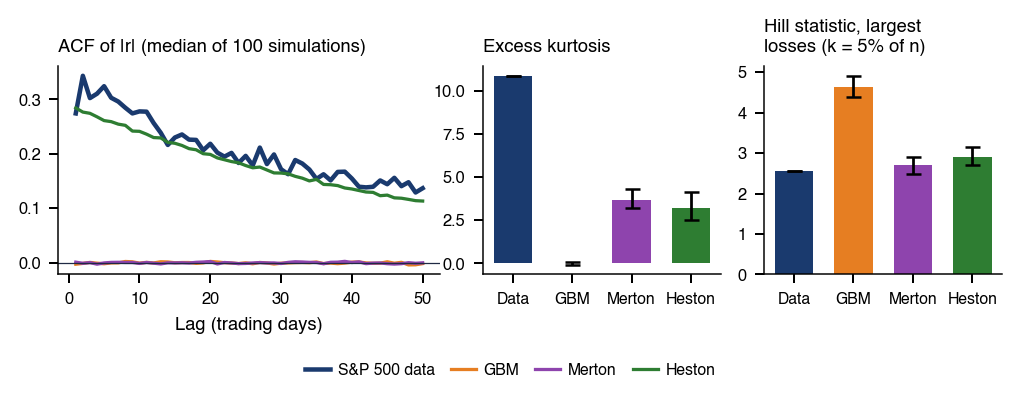
 MFM_ch11_donsker
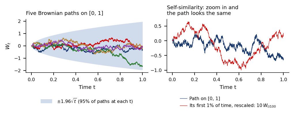
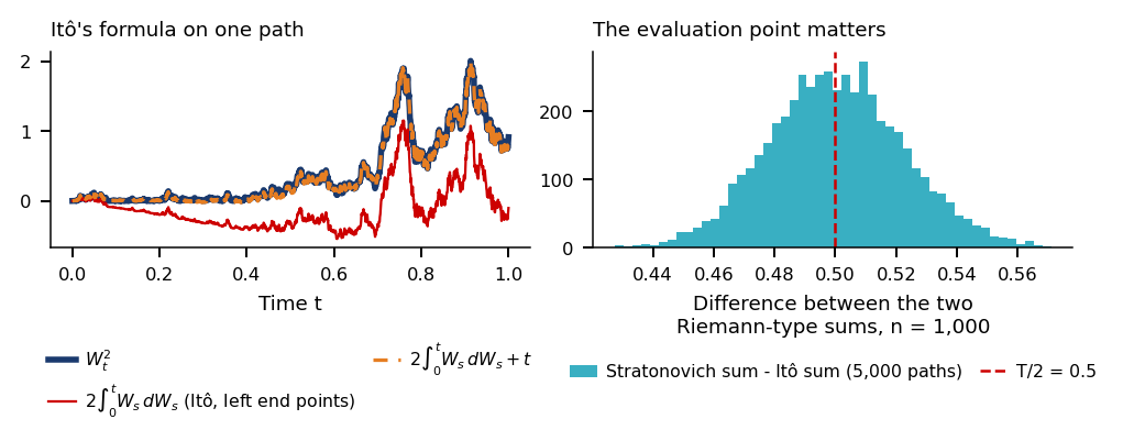
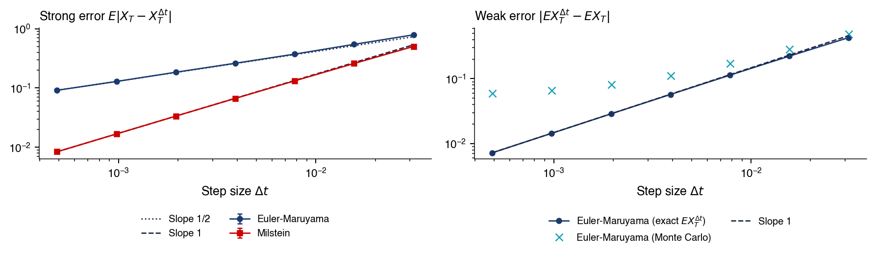
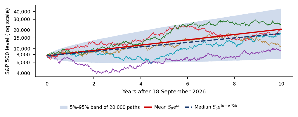
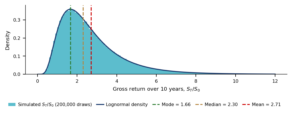
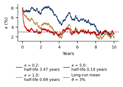
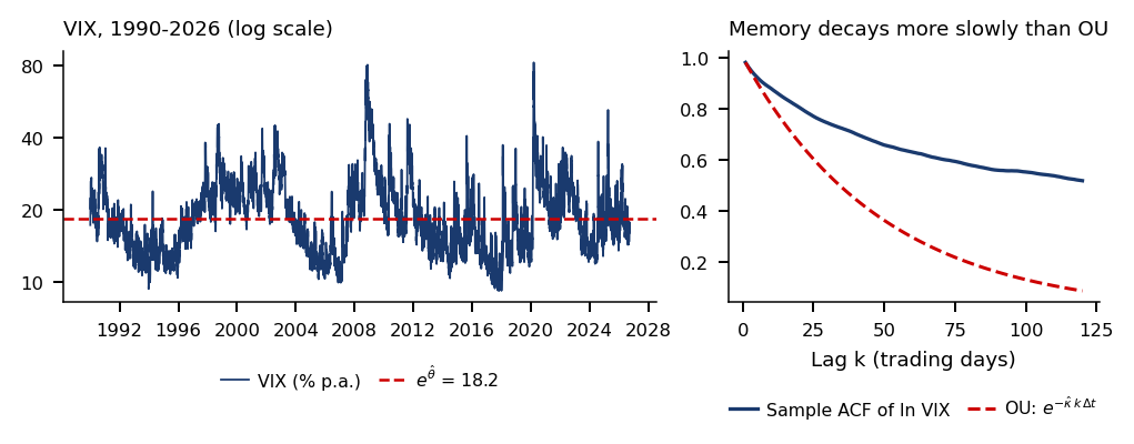
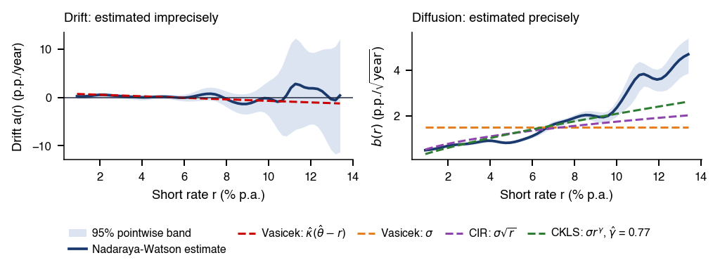
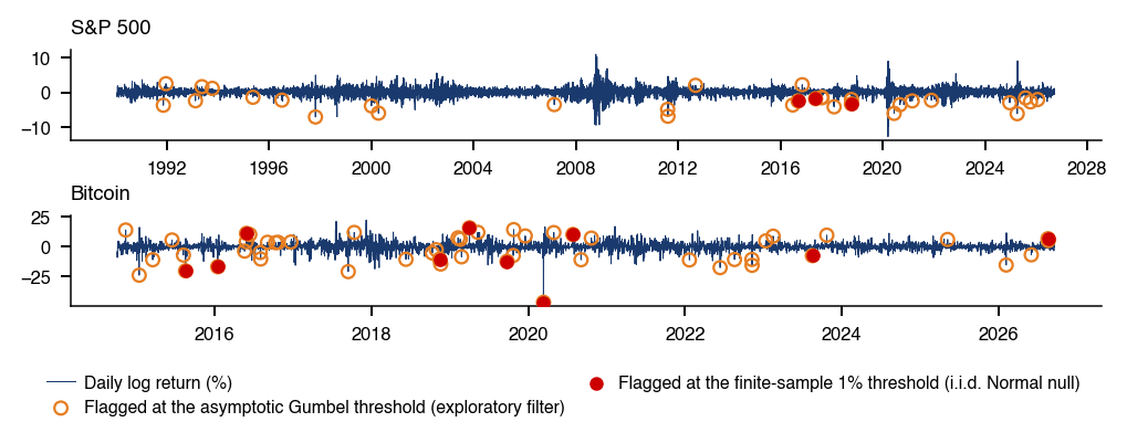
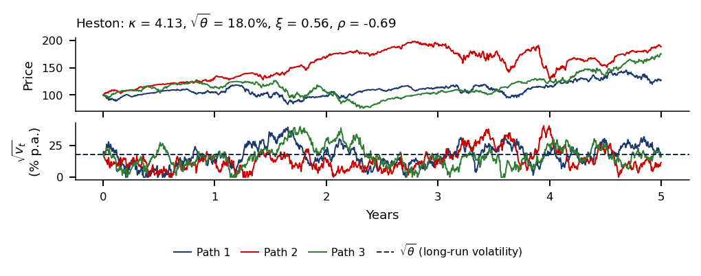
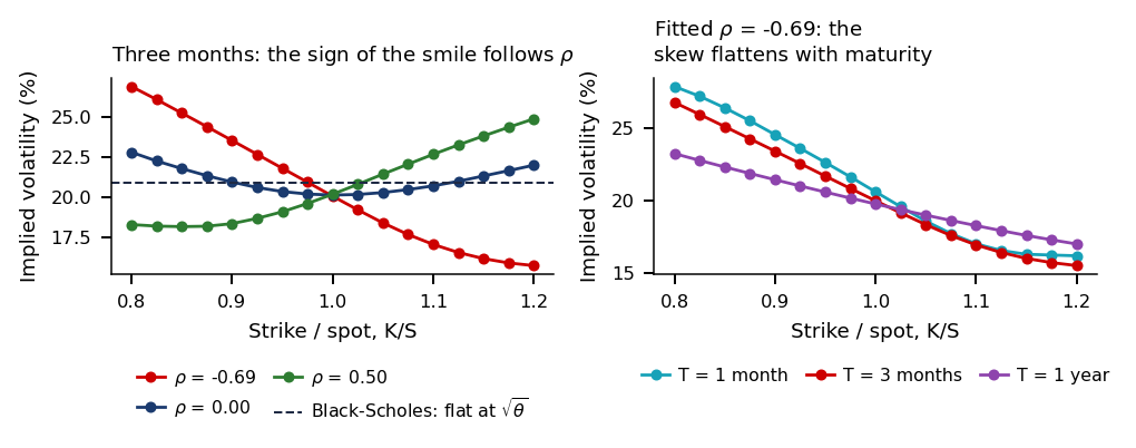
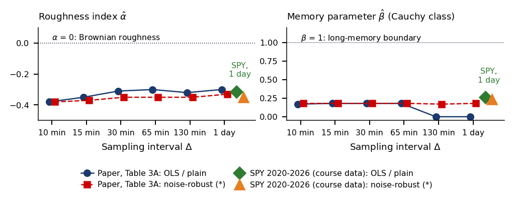



 Applied Computational Finance