Bucharest University of Economic Studies IDA Institute Digital Assets Blockchain Research Center AI4EFin Artificial Intelligence for Energy Finance Romanian Academy, Institute for Economic Forecasting MSCA Digital Finance
“Hundreds of papers and factors attempt to explain the cross-section of expected returns. Given this extensive data mining, it does not make sense to use the usual criteria for establishing significance.” — Harvey, Liu & Zhu (2016)
After hundreds of factors tried on the same data, a new factor needs \(t > 3\), not \(t > 2\)
5-day direction of the S&P 500 (Standard & Poor's), \(n = 6{,}269\): no model beats the “always up” benchmark
the benchmark has 58.1% accuracy; the logit has 57.7% and predicts “up” on 98.3% of days
Walk-forward backtest 2010–2026: the Sharpe ratio of the GBM (Gradient Boosting Machine) strategy is 0.33
the Sharpe ratio of buy-and-hold is 0.66
On a target with nothing to predict, shuffled K-fold reports 69.4% accuracy
Hundreds of papers and factors attempt to explain the cross-section of expected returns. Given this extensive data mining, it does not make sense to use the usual criteria for establishing significance.
Harvey, Liu & Zhu (2016) show that, once hundreds of factors have been tried on the same data, the usual hurdle \(t > 2\) no longer separates discoveries from the luck of selection: a new factor needs \(t > 3\). Machine learning brings flexible, nonlinear functional forms and hundreds of candidate predictors to finance, and with them the same problem on a larger scale. Financial data have a very low signal-to-noise ratio and a single, serially dependent history. On daily S&P 500 (Standard & Poor's) returns over 2000–2026, the autocorrelations of returns are small, the lag-1 autocorrelation is \(-0.099\), while the autocorrelations of absolute returns are large and persistent: risk has predictable structure, direction hardly any.
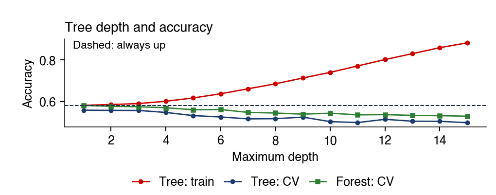
The chapter's case study asks the question directly: can the 5-day direction of the S&P 500 be predicted? On 6,269 daily observations, four models (a penalised logit, a random forest, gradient boosting and a neural network) are validated on the same 5 folds, with purging and embargo. No model beats the "always up" benchmark, whose accuracy is 58.1%. The logit reaches 57.7% accuracy because it predicts "up" on 98.3% of days. In the 2010–2026 walk-forward backtest, the GBM (Gradient Boosting Machine) strategy has a Sharpe ratio of 0.33 and buy-and-hold 0.66.
Most false results come from the process, not the algorithm. On a target with nothing to predict, K-fold with shuffled observations reports 69.4% accuracy, purged K-fold with embargo 49.6%. On a grid of 1,284 Bitcoin trading rules, the selected rule has a Sharpe ratio of 2.02 in-sample and 0.03 out-of-sample. The chapter therefore builds, step by step, the features, labels, validation and tests that separate a real prediction from the best of many trials.
Accuracy and AUC (area under the ROC curve) of the four models for the 5-day direction of the S&P 500, mean over the 5 purged folds, with whiskers of \(\pm 1\) standard deviation across folds; the "always up" benchmark has 58.1% accuracy, and AUC \(= 0.5\) means no skill. Interactive chart: “Model Comparison: Fold Means” →
What you will be able to do
Compute features and labels without look-ahead bias.
Compute the score of a model validated with purging and embargo.
Derive why truncated fixed-width window fractional differencing (FFD) of an \(I(1)\) price stays \(I(1)\).
Interpret the tests of a classifier and of a backtest against a benchmark.
Machine learning (ML) estimates a prediction function from data with few restrictions on its form. The chapter applies it to financial returns, where the signal is weak and the history is short and serially dependent. Two failures of the research process dominate in this setting (López de Prado, 2018).Look-ahead bias is the use of information that was not available at the decision date. Selection bias is the reporting of the best of many trials as if it were the only one. The first section separates what is predictable in a return series from what is not, and states what a small predictive gain is worth.
compute the score of a model validated with purging and embargo
derive why truncated FFD (Fixed-width window Fractional Differentiation) of an \(I(1)\) price stays \(I(1)\)
interpret, against a benchmark, the Pesaran–Timmermann (PT) and Diebold–Mariano (DM) tests, the deflated Sharpe ratio (DSR), the superior predictive ability (SPA) test and the probability of backtest overfitting (PBO)
Further Topics and Appendix: reading for familiarity
Detailed examples and advanced topics are in Further Topics, after the Conclusions
the footer button leads there; the Back button returns to the starting slide
Most failures come from the process, not the algorithm (López de Prado (2018)); two failures dominate
look-ahead bias: using information not available at decision time
The diagram shows the stages that turn raw prices into a claim that can be tested. Prices are sampled into bars, daily bars in this chapter. Features are computed from the bars with information available at the decision date only, and some of them keep part of the memory of the price level. Labels define what the model learns: the triple-barrier label and the meta-label are two alternatives to the plain sign of a future return. The models are the least absolute shrinkage and selection operator (LASSO), the random forest (RF), the gradient boosting machine (GBM) and the multilayer perceptron (MLP).
The second row of the diagram is where most errors are caught or missed. Validation uses purged cross-validation (CV) with an embargo, which keeps the training and test sets from sharing information. A predicted direction becomes a trade only in a backtest with costs, and the backtest becomes evidence only after formal inference. The chapter uses the Diebold–Mariano (DM) test, the superior predictive ability (SPA) test, the deflated Sharpe ratio (DSR) and the probability of backtest overfitting (PBO). Deployment and monitoring close the chain.
Each stage answers a narrow question. Features must use only information available at the decision date. Validation measures what still holds on observations the model has not seen. Inference decides whether a difference from a benchmark is larger than sampling error and the cost of trading.
Flexible, non-linear functional forms find interactions between predictors without the analyst specifying them.
Hundreds of candidate predictors are available, the "factor zoo" of Chapter 3.
Alternative data, such as text, images, order books and on-chain data, add further predictors.
The constraints are as strong. The signal-to-noise ratio of returns is very low, and there is a single, serially dependent history that cannot be re-run. Markets are non-stationary: regimes change, structural breaks occur and prices react to the behaviour of market participants. Labels are not given but must be constructed, and errors cost real money. Together these features create a large risk of overfitting, that is, of fitting noise.
The Adaptive Markets Hypothesis of Lo (2004) describes predictability as transient: it appears, is arbitraged away and re-appears. A model that worked yesterday is therefore a hypothesis, not a law; market efficiency is the subject of Chapter 2. The hard part of the work is not fitting a model but not fooling oneself, which requires correct labels, correct validation and honest backtests.
In brief
The promise
Flexible, non-linear functional forms
interactions found automatically
Hundreds of candidate predictors (the “factor zoo”, Chapter 3)
Alternative data: text, images, order books, on-chain data
The constraints
Very low signal-to-noise ratio
one serially dependent history that cannot be re-run
Which part of a financial series is predictable can be seen first in its autocorrelations. The autocorrelation at lag \(k\) is
\[\rho_k = \mathrm{Corr}(x_t, x_{t-k}),\]
(13.1)
computed here for the daily log return \(r_t = \log P_t - \log P_{t-1}\) and for its absolute value \(|r_t|\), where \(P_t\) is the closing price on day \(t\). Under the hypothesis of no autocorrelation, each estimate \(\hat\rho_k\) lies within \(\pm 1.96/\sqrt{T}\) with probability 95%, where \(T\) is the number of observations. For \(|r_t|\) the band requires a finite fourth moment, which Chapter 1 questions.
On the S&P 500, the autocorrelations of returns are smaller than those of absolute returns. Even so, 13 of the 40 return autocorrelations lie outside the band, and at lag 1 the estimate is \(\hat\rho_1 = -0.099\). Three qualifications apply. The band is not simultaneous over 40 lags; it is not robust to heteroskedasticity; and a coefficient outside the band does not show that a trading rule is profitable after costs.
The autocorrelations of \(|r_t|\) are large and persistent. The magnitude of returns, that is, risk, has predictable structure, while their direction has very little. ML therefore has its best chance where such structure exists: volatility, risk, liquidity and the cross-sectional ranking of assets.
In brief
The question: which part of a financial series is predictable at all?
Autocorrelation at lag \(k\): \(\rho_k = \Corr(x_t, x_{t-k})\)
for the daily log return \(r_t = \log P_t - \log P_{t-1}\) and for \(|r_t|\)
Next chart: lag \(k\) on the horizontal axis, \(\hat\rho_k\) on the vertical axis
blue bars for \(r_t\), brown bars for \(|r_t|\)
The light-blue band, \(\pm 1.96/\sqrt{T}\), is the 95% band under no autocorrelation
\(T\): number of observations
for \(|r_t|\), the band requires a finite fourth moment, which Chapter 1 questions
Autocorrelations of returns \(r_t\) are smaller than those of \(|r_t|\), yet 13 of the 40 lie outside the band
at lag 1, \(\hat\rho_1 = -0.099\)
the band is neither simultaneous over 40 lags nor robust to heteroskedasticity
leaving the band does not show profitability after costs
Autocorrelations of \(|r_t|\) are large and persistent
The chart shows the lag \(k\) on the horizontal axis and the estimated autocorrelation \(\hat\rho_k\) on the vertical axis. Blue bars are the autocorrelations of \(r_t\), brown bars those of the transformed series, and the light-blue band is \(\pm 1.96/\sqrt{T}\), the 95% band under no autocorrelation. The first slider sets the power \(p\) in \(|r_t|^p\):\(p = 1\) gives absolute returns and \(p = 2\) squared returns. The menu restricts the sample to 2000–2012 or 2013–2026, and the ▶ button moves the power step by step.
Question for the room For the S&P 500 over 2000–2026, daily-return autocorrelations are small at most lags. What do the autocorrelations of absolute returns |r_t| look like?
Answer
For |r_t|, autocorrelation is 0.29 at lag 1 and 0.16 at lag 40; all 40 lie outside the ±0.024 band. For returns, the first-order autocorrelation is −0.10, and 13 of 40 lie outside the band. Low linear autocorrelation does not imply independence, and taking absolute values does not simply square the ACF. The result indicates persistence in return magnitudes. The ±0.024 band is a pointwise i.i.d. reference, not a simultaneous band robust to heteroskedasticity.
At \(p = 1\) over 2000–2026, the bars of \(|r_t|\) are large and decline slowly with the lag, while the bars of \(r_t\) are small, with \(\hat\rho_1 = -0.099\) and 13 of 40 outside the band. Changing the power changes the height of the brown bars but not their persistence: the predictable structure lies in the magnitude of returns, not in their sign.
The broadest comparison of ML methods for returns is that of Gu, Kelly & Xiu (2020). They use monthly returns of individual US (United States) stocks over 1957–2016 and compare linear models, penalised regressions, principal component regression (PCR), partial least squares (PLS), random forests, gradient boosting and neural networks. Their measure of fit is the out-of-sample (OOS) \(R^2\),
where \(r_t\) is the realised return in month \(t\) of the test period and \(\hat r_t\) the forecast made with information up to \(t-1\). The denominator in (13.2) is the squared error of the zero forecast \(\hat r_t = 0\):\(R^2_{OOS} > 0\) when the model beats it and \(R^2_{OOS} < 0\) when it does worse.
The monthly values in their Table 1 are small. A three-layer network reaches 0.40%, gradient boosting 0.34% and a random forest 0.33%. Ordinary least squares (OLS) with 3 predictors reaches 0.16%, while OLS with all 900+ predictors gives −3.46%. Trees and networks win through non-linear interactions, and the dominant predictors are momentum, liquidity and volatility.
Returns have almost no predictable direction, while their magnitude is strongly persistent. Out-of-sample gains for return forecasts are measured in tenths of a percent of \(R^2\), and their size depends on the benchmark, the zero forecast or the historical mean. The next section introduces the models that produce such forecasts and the penalties that keep their variance under control.
Machine Learning Methods
The toolbox has three parts:
a loss that measures the error of a prediction;
a penalty that limits the complexity of the fitted function;
a validation scheme that chooses the strength of the penalty.
Five model families fill it: penalised linear models, single trees, random forests, gradient boosting and neural networks. With a weak signal, controlling the variance of the estimate matters more than adding flexibility, and the bias–variance decomposition makes this precise.
Here \((y_i, \mathbf{x}_i)\),\(i = 1,\dots,n\), are the target and the feature vector of observation \(i\), and \(\mathcal{F}\) is the model family, for example all trees of depth 3. The loss \(L\) is the squared error \((y - f)^2\) or, for a probability \(f\) that \(y = 1\), the log-loss \(-[y\log f + (1-y)\log(1-f)]\). The term \(\Omega(f)\) penalises complexity with weight \(\lambda \ge 0\):\(\lambda = 0\) means no penalty, and a large \(\lambda\) gives a simpler model.
The weight \(\lambda\) cannot be chosen by (13.3) itself, since the training loss always prefers \(\lambda = 0\). It is chosen by \(K\)-fold cross-validation on folds \(\mathcal{P}_1, \dots, \mathcal{P}_K\):
where \(n_k\) is the number of observations in fold \(k\) and \(\hat f^{(-k)}_\lambda\) the model fitted on the other \(K-1\) folds. Each observation is predicted by a model that has not seen it. Whether this is enough for financial series, whose neighbouring observations share information, is the subject of the section on honest validation.
In brief
The question of this section
why, with a weak signal, does variance control matter more than flexibility?
Supervised learning picks, within a model family, the function that fits the training data best
\((y_i, \mathbf{x}_i)\), \(i = 1,\dots,n\): target and feature vector of observation \(i\); \(\mathcal{F}\): the model family (e.g. all trees of depth 3)
\(L\): loss, the squared error \((y - f)^2\) or, for a probability \(f\) of \(y = 1\), the log-loss \(-[y\log f + (1-y)\log(1-f)]\)
\(\Omega(f)\): complexity penalty with weight \(\lambda \ge 0\); \(\lambda = 0\): no penalty, large \(\lambda\): a simpler model
\(\lambda\) is chosen by \(K\)-fold cross-validation (CV) on folds \(\mathcal{P}_1, \dots, \mathcal{P}_K\):
The reason for penalising is the decomposition of the expected test error, derived in Chapter 7 of Hastie, Tibshirani & Friedman (2009). Let \(y = f(\mathbf{x}) + \varepsilon\) with \(\mathbb{E}[\varepsilon] = 0\) and \(\mathrm{Var}(\varepsilon) = \sigma^2\). At a point \(\mathbf{x}_0\),
where the expectation is over possible training samples and over the noise of the new observation \(y_0 = f(\mathbf{x}_0) + \varepsilon_0\). The three terms are the noise, the squared bias and the variance. The bias is the systematic error of a family that is too simple. The variance is the sensitivity of \(\hat f\) to the training sample, and it grows with the flexibility of the model. The noise \(\sigma^2\) is the variance of the unpredictable part of \(y\), which no model can reduce.
The derivation adds and subtracts \(\mathbb{E}[\hat f(\mathbf{x}_0)]\) in \(y_0 - \hat f(\mathbf{x}_0)\) and expands the square. The cross terms have mean zero because \(\varepsilon_0\) is independent of the training sample.
In finance, return forecasts reduce the error very little. An out-of-sample \(R^2\) below 1% means that the model removes less than 1% of the squared loss of the benchmark. This does not identify \(\sigma^2\), because the remaining error also contains misspecification, omitted variables and estimation error. It does explain the design of the models that follow: penalties and the averaging of trees reduce variance at the price of a small bias.
Penalised regressions apply (13.3) to a linear model with \(p\) standardised features and coefficients \(\boldsymbol\beta = (\beta_1, \dots, \beta_p)\):
with \(\|\boldsymbol\beta\|_1 = \sum_j |\beta_j|\),\(\|\boldsymbol\beta\|_2^2 = \sum_j \beta_j^2\) and \(\alpha \in [0,1]\) the share of the absolute-value penalty. Ridge regression, \(\alpha = 0\)(Hoerl & Kennard, 1970), has the closed form \(\hat{\boldsymbol\beta} = (\mathbf{X}^\top\mathbf{X} + \tfrac{n\lambda}{2}\mathbf{I})^{-1}\mathbf{X}^\top\mathbf{y}\). It shrinks all coefficients, none exactly to zero, and stabilises the estimate when predictors are correlated.
The LASSO, \(\alpha = 1\)(Tibshirani, 1996), uses the penalty \(|\beta_j|\), which has a kink at zero. As a result some coefficients become exactly zero, and the LASSO selects features. The elastic net, \(0 < \alpha < 1\)(Zou & Hastie, 2005), keeps groups of correlated predictors together, whereas the LASSO arbitrarily keeps one of them.
The chapter's linear benchmark is the penalised logit. It models the probability \(p = P(y = 1 \mid \mathbf{x}) = 1/(1+e^{-\mathbf{x}^\top\boldsymbol\beta})\) and replaces the squared loss in (13.6) by the log-loss.
In brief
Penalised regressions, with \(p\) standardised features and coefficients \(\bm\beta = (\beta_1, \dots, \beta_p)\):
A classification tree splits the feature space recursively. At each node \(v\) it chooses the feature \(j\) and the threshold \(s\) that reduce the Gini impurity \(G = 1 - \sum_c \hat\pi_c^2\) the most:
\[(j^*, s^*) = \arg\min_{j,\,s}\ \Big[\frac{n_L}{n_v}\,G(L) + \frac{n_R}{n_v}\,G(R)\Big], \qquad L = \{x_j \le s\},\ R = \{x_j > s\}.\]
(13.7)
Here \(\hat\pi_c\) is the share of class \(c\) in the node, and \(n_v\),\(n_L\),\(n_R\) are the numbers of observations in the node and in its two children. A pure node has \(G = 0\). With two classes \(G = 2\hat\pi(1-\hat\pi)\), which reaches its maximum of 0.5 at a 50/50 split. A leaf predicts the share of class 1 among its observations.
A random forest (RF) (Breiman, 2001) averages \(B\) trees, \(\hat f_{RF}(\mathbf{x}) = \frac1B\sum_{b=1}^{B} T_b(\mathbf{x})\). Each tree \(T_b\) is grown on a bootstrap sample, with a random subset of features considered at each split. If one tree has variance \(\sigma_T^2\) and two trees have correlation \(\rho\), Chapter 15 of Hastie, Tibshirani & Friedman (2009) gives
More trees remove the second term of (13.8) but not the first. The random feature subsets lower \(\rho\), the only term that more trees cannot remove. The out-of-bag error of the forest, computed on the observations left out of each bootstrap sample, is optimistic when labels overlap.
In brief
Trees: at each node \(v\) choose the feature \(j\) and threshold \(s\) that reduce the Gini impurity the most
Gini impurity: \(G = 1 - \sum_c \hat\pi_c^2\)
\[
(j^*, s^*) = \arg\min_{j,\,s}\ \Big[\frac{n_L}{n_v}\,G(L) + \frac{n_R}{n_v}\,G(R)\Big], \qquad L = \{x_j \le s\},\ R = \{x_j > s\}
\]
\(\hat\pi_c\): share of class \(c\) in the node; \(n_v\), \(n_L\), \(n_R\): observations in the node and in its two children
\(G = 0\) for a pure node; with two classes \(G = 2\hat\pi(1-\hat\pi)\), at most \(0.5\) at 50/50; a leaf predicts the share of class 1
Random forest (RF, Breiman (2001)): \(\hat f_{RF}(\mathbf{x}) = \frac1B\sum_{b=1}^{B} T_b(\mathbf{x})\)
each tree \(T_b\) grown on a bootstrap sample with a random subset of features at each split
The gradient boosting machine (GBM) (Friedman, 2001) builds the model step by step, adding at each step a small tree that corrects the errors of the current model:
\(F_m\) is the model after \(m\) steps, \(h_m\) the tree fitted to the pseudo-residuals \(r_{im}\) and \(\eta \in (0, 1]\) the learning rate. For the log-loss on the logit score, the pseudo-residual is \(r_{im} = y_i - \hat p_{m-1}(\mathbf{x}_i)\), the difference between the outcome and the current predicted probability. A small \(\eta\) learns slowly and overfits less.
The multilayer perceptron (MLP) stacks hidden layers \(\mathbf{h}^{(\ell)} = g(\mathbf{W}^{(\ell)}\mathbf{h}^{(\ell-1)} + \mathbf{b}^{(\ell)})\), starting from \(\mathbf{h}^{(0)} = \mathbf{x}\), and ends with the output \(\hat p = 1/(1 + e^{-(\mathbf{w}^\top\mathbf{h}^{(D)} + b)})\).\(\mathbf{W}^{(\ell)}\) and \(\mathbf{b}^{(\ell)}\) are the weights and biases of layer \(\ell\),\(D\) is the number of hidden layers, and \(g(z) = \max(0, z)\) is the rectified linear unit (ReLU), applied element by element. The weights minimise the log-loss by gradient descent.
The MLP is regularised by early stopping. A chronological validation set, the last 10% of the training data, purged, is held out, and training stops when the validation log-loss stops falling. Richer architectures are treated in Chapter 14.
\(F_m\): the model after \(m\) steps; \(h_m\): the tree fitted to the pseudo-residuals \(r_{im}\); for the log-loss on the logit score, \(r_{im} = y_i - \hat p_{m-1}(\mathbf{x}_i)\)
\(\eta \in (0, 1]\): learning rate; a small \(\eta\) learns slowly and overfits less
the output: \(\hat p = 1/\big(1 + e^{-(\mathbf{w}^\top\mathbf{h}^{(D)} + b)}\big)\)
\(\mathbf{W}^{(\ell)}\), \(\mathbf{b}^{(\ell)}\): weights and biases of layer \(\ell\); \(D\): number of hidden layers; \(g(z) = \max(0, z)\): the ReLU (rectified linear unit), element by element
the weights minimise the log-loss by gradient descent
early stopping: a chronological validation set (the last 10% of the training data, purged); training stops when the validation log-loss stops falling
The regularisation path shows the coefficients of a penalised model as functions of the penalty. The model is an \(L_1\)-penalised logistic regression for the 5-day direction of the S&P 500 with 14 standardised features, those of the case study. In the left chart, the horizontal axis is the penalty \(\lambda = 1/C\) on a log scale, with the stronger penalty to the left, and the vertical axis is the standardised coefficient of each feature. The right chart shows the coefficients at the penalty chosen with the slider.
The menu switches between the LASSO (\(L_1\)) and ridge (\(L_2\)) penalties. The slider moves the penalty from strong to weak, and the ▶ button runs it along the path. Under the LASSO, coefficients leave zero one at a time as the penalty weakens; under ridge, all coefficients are non-zero and shrink together.
Question for the room On the LASSO path fitted to the full sample, which feature first becomes non-zero as the penalty decreases?
Answer
The first feature is ffd_price. vol_20 has the largest absolute coefficient at a weak penalty, which does not determine entry order. First-order return autocorrelation does not determine it either. The truncated FFD filter retains a component proportional to the log-price level. Early entry does not establish predictive skill: mean purged-CV AUC, with the scaler estimated in each fold, ranges from 0.476 to 0.486 across penalties with at least one non-zero coefficient.
Under a strong penalty every coefficient is zero. The first feature to enter is the FFD log price, ffd_price. Under a weak penalty the volatility features receive the largest coefficients. All coefficients remain small in absolute value, which is what a weak signal looks like.
The chart labels refer to the features of the case study. vol_20, vol_60 and vol_ratio are the 20- and 60-day volatilities and their ratio; mom_20 and mom_60 are the log returns over the last 20 and 60 days; ffd_price is the log price after fixed-width window fractional differentiation (FFD).
Under a strong penalty, at the left of the chart, every coefficient is zero. The first feature to enter is the FFD log price, which the next section shows to be a scaled price level. Under a weak penalty the volatility features get the largest coefficients.
All coefficients are small in absolute value, consistent with a weak signal in a nearly efficient market. The order of entry describes the penalty, not the predictive value of a feature; whether a selected variable has a significant effect is a separate question, treated in the section on machine learning for inference.
In brief
\(L_1\)-penalised logistic regression for the 5-day direction of the S&P 500, 14 standardised features
Chart labels
vol_20, vol_60, vol_ratio: the 20- and 60-day volatilities and their ratio
mom_20, mom_60: the log returns over the last 20 and 60 days
ffd_price: the FFD log price
Horizontal axis: the penalty \(\lambda = 1/C\), on a log scale, stronger to the left
vertical axis: the standardised coefficient
Strong penalty (left of the chart): every coefficient is zero
the first feature to enter is the FFD (fixed-width window fractional differentiation) log price
FFD log price: a scaled price level (next section)
Weak penalty: the volatility features get the largest coefficients
All coefficients are small in absolute value
weak signal, consistent with near-efficient markets
Penalised linear models, trees, forests, boosting and neural networks all minimise a loss plus a penalty, and differ in the family \(\mathcal{F}\) and the form of \(\Omega\). With an out-of-sample \(R^2\) below 1%, the variance term of (13.5) is the one to control, and shrinkage and averaging are the main tools. The LASSO path on the S&P 500 shows small coefficients and an early entry of the FFD log price, whose construction is the subject of the next section.
Features: Fractional Differencing and Its Limitations
A feature should be stationary, so that a relation learnt on the past can hold in the future, yet differencing a price into returns erases the memory of its level. Fractional differencing, proposed for this purpose by López de Prado (2018), differences by less than one. This section defines the fixed-width window version, applies the proposed rule for choosing the order \(d\) to the S&P 500 and shows why the result is still a non-stationary series.
Stationarity, Memory and the Fractional Difference (1/2)
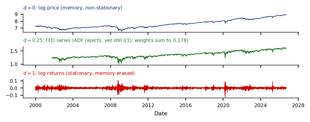
Log prices \(X_t = \log P_t\), with \(P_t\) the closing price on day \(t\), behave as \(I(1)\) series. Returns \(\Delta\log P_t = \log P_t - \log P_{t-1}\) are \(I(0)\), but they erase the memory of the price level. The question is how to turn a price into a stationary feature without erasing that memory.
The integration order is defined with the backshift operator \(B\),\(BX_t = X_{t-1}\). A series \(X_t\) is \(I(\delta)\) if \((1-B)^{\delta}X_t\) is \(I(0)\), that is, stationary with short memory. An \(I(1)\) series is of the random-walk type and becomes stationary after one difference. The order \(\delta\) may be fractional: the series is then stationary only for \(\delta < \tfrac12\), with long memory when \(0 < \delta < \tfrac12\)(Hosking, 1981).
Fractional differencing applies \((1-B)^d\) with a non-integer \(d\), differencing by less than 1. The aim is to remove the unit root while keeping part of the memory of the level, which ordinary returns, \(d = 1\), discard.
In brief
The question of this section
how do we turn a price into a stationary feature without erasing its memory?
Log prices \(X_t = \log P_t\) behave as \(I(1)\)
\(P_t\): closing price on day \(t\)
Returns \(\Delta\log P_t = \log P_t - \log P_{t-1}\) are \(I(0)\) but erase the memory of the price level
Integration order: a series \(X_t\) is \(I(\delta)\) if \((1-B)^{\delta} X_t\) is \(I(0)\)
\(B\): backshift operator, \(B X_t = X_{t-1}\)
\(I(0)\): stationary with short memory; \(I(1)\): a random walk type series, stationary after one difference
\(\delta\) may be fractional: the series is stationary only for \(\delta < \tfrac12\), with long memory when \(0 < \delta < \tfrac12\) (Hosking (1981))
Idea of fractional differencing: difference by less than 1
removing the unit root while keeping part of the memory
Stationarity, Memory and the Fractional Difference (2/2)
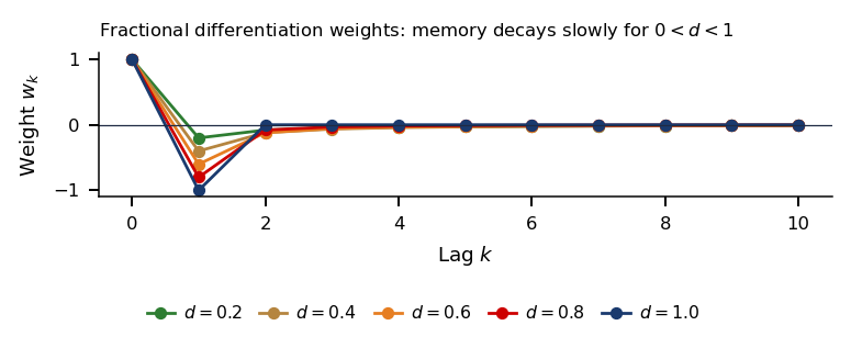
Here \(d\) is the differencing order chosen by the analyst, \(k\) the lag in days and \(w_k\) the weight of the value \(k\) days back. For \(d = 1\) the weights are \((1, -1, 0, \dots)\), ordinary returns. For \(0 < d < 1\) the weights decay hyperbolically, so distant values keep a non-zero weight and memory is kept.
An \(I(1)\) log price differenced with order \(d\) is \(I(1-d)\). It is therefore still non-stationary for \(d \le \tfrac12\), and stationary with long memory for \(\tfrac12 < d < 1\). The infinite weights in (13.10) sum to \((1-1)^d = 0\), so the level cancels, but only in the limit; the asymptotics of the weights are in the Appendix.
López de Prado (2018) proposes the minimum \(d\) at which an Augmented Dickey–Fuller (ADF) unit-root test rejects. The test equation and its critical value come two slides later, and the rest of the section shows why this rule fails.
In brief
Definition (Fractional difference of order \(d\)).
\(\tilde X_t = (1-B)^d X_t = \sum_{k=0}^{\infty} w_k X_{t-k}\), with \(w_0 = 1\) and \(w_k = -\,w_{k-1}\,\frac{d-k+1}{k}\)
Notation
\(d\): differencing order chosen by the analyst; \(k\): lag in days
\(w_k\): weight of the value \(k\) days back, from the binomial expansion of \((1-B)^d\)
The infinite sum in (13.10) cannot be computed on a finite sample. Fixed-width window fractional differentiation (FFD) truncates the weights (López de Prado, 2018): it keeps \(w_0, \dots, w_K\) with \(|w_k| \ge \tau\), for example \(\tau = 10^{-4}\), and drops the rest, so that
\[\tilde X_t = \sum_{k=0}^{K} w_k X_{t-k}, \qquad t > K.\]
(13.11)
\(\tau\) is the smallest weight kept and \(K\) the last lag kept, that is, the window length. The first \(K\) days have too little history and are dropped.
Every \(\tilde X_t\) uses the same number of lags, and only past values enter, so the feature has no look-ahead. The price of the truncation is the window length: the smaller \(d\), the more lags are needed. At \(d = 0.25\) and \(\tau = 10^{-4}\), the window has \(K = 444\) lags.
The truncated weights no longer sum to zero. Their sum is 0.178 at \(d = 0.25\) and 0.040 at \(d = 0.5\). This number decides the integration order of the FFD series, as the last slide of the section shows.
The null hypothesis is \(\gamma = 0\), a unit root. The \(p\) lagged differences absorb the autocorrelation of \(e_t\). With a constant, the test rejects \(H_0\) at 5% when the statistic is below about \(-2.86\).
The rule of López de Prado (2018) computes the FFD series on a grid of \(d\) between 0 and 1 and picks the smallest \(d\) at which the ADF test rejects. The chosen order is then meant to give a stationary feature with as much memory as possible.
The next chart puts \(d\) on the horizontal axis. The ADF statistic is drawn in blue on the left axis, and the correlation of the FFD series with the log price in green on the right axis. The red dashed line is the 5% critical value, and the vertical line marks \(d^* = 0.25\).
In brief
Augmented Dickey–Fuller (ADF) unit-root test: the \(t\)-statistic of \(\gamma\) in
The left chart is the ADF statistic as a function of \(d\), with the 5% critical value; the right chart shows the FFD series at the chosen \(d\) together with the log price. The slider sets the differencing order \(d\), and the menu sets the lags of the ADF test: one lag, or the number chosen by the Akaike information criterion (AIC). The ▶ button raises \(d\) step by step.
Question for the room At d = 0.25, ADF with one lag rejects the unit root. Is this rejection sufficient to treat the FFD series as stationary?
Answer
ADF with one lag rejects: −2.96 < −2.86. With 34 AIC-selected lags, the statistic is −0.72 and does not reject. Neither decision is a proof. The structural argument is that, for an I(1) log price, a finite filter whose weights sum to 0.178 retains the I(1) component. The 0.98 correlation with the log price is a warning sign, not a stationarity test.
With one lag, the ADF statistic falls below the critical value from \(d = 0.25\), where it equals \(-2.96\); at that order the FFD series has a correlation of 0.98 with the log price. With the lags chosen by the AIC, the same series does not reject. The right chart shows why the verdict is fragile: at \(d^*\) the FFD series still follows the trend of the price.
For the S&P 500 log price over 2000–2026, the ADF regression with a constant and one lag gives \(-2.96\) at \(d = 0.25\), below the critical value. The rule therefore rejects from \(d = 0.25\). At that order the correlation between the FFD series and the log price is \(\mathrm{Corr}(\tilde X_t, \log P_t) = 0.98\): the FFD series is almost the log price.
The same series, tested with 34 lags chosen by the AIC, gives an ADF statistic of \(-0.72\), and the unit root is not rejected. The verdict thus depends on the number of lags. A correlation of 0.98 with an \(I(1)\) price is a warning, not a virtue.
What the result supports is a comparison of procedures: the same log price, two lag choices and two verdicts. It does not establish that the FFD series at \(d = 0.25\) is stationary.
The first term is today's level times the sum of the truncated weights. The second is a weighted sum of the \(k\)-day changes \(X_t - X_{t-k}\). If \(X_t\) is \(I(1)\), each change is \(I(0)\), and so is their finite weighted sum. The first term is \(0.178\,X_t\) at \(d = 0.25\): a scaled random walk. The FFD series is therefore \(I(1)\).
The unit-root component has small variance next to the stationary part, so an ADF test with few lags confuses the two. A Monte Carlo experiment measures the size of the problem. For a pure random walk of \(T = 6{,}274\) days, filtered by FFD with \(d = 0.25\), the ADF test with one lag rejects the unit root in 97.8% of 500 samples, at a nominal level of 5%.
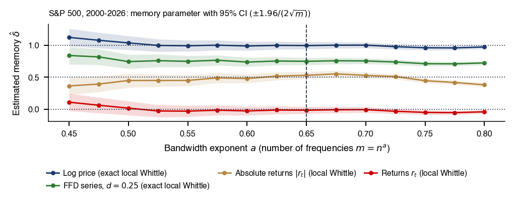
The general statement is that a finite filter whose weights do not sum to zero keeps a level component, whatever the ADF \(p\)-value. The FFD log price in the case study is therefore a scaled price level, not a stationary feature. The memory of the series is measured directly, with the local Whittle estimator, in Further Topics.
first term: today's level times the sum of the truncated weights; second term: a weighted sum of the \(k\)-day changes \(X_t - X_{t-k}\)
If \(X_t\) is \(I(1)\), each \(X_t - X_{t-k}\) is \(I(0)\)
the first term is \(0.178\, X_t\) at \(d = 0.25\): a scaled random walk
The unit-root component has small variance next to the stationary part
so ADF with few lags confuses the two
Monte Carlo: pure random walk, \(T = 6{,}274\) days (the length of the S&P 500 FFD series), FFD with \(d = 0.25\): ADF (1 lag) rejects in 97.8% of 500 samples, at a nominal 5%
A finite filter whose weights do not sum to zero keeps a level component, whatever the ADF p-value
Consequence: the FFD log-price in the case study is a scaled price level, not a stationary feature
Truncated fractional differencing of an \(I(1)\) price keeps the level with weight \(\sum_{k \le K} w_k\), 0.178 at \(d = 0.25\), and the series remains \(I(1)\). The ADF-based rule for choosing \(d\) rejects with one lag and not with 34, and on a pure random walk it rejects in 97.8% of samples at a nominal 5%. The long memory of the S&P 500 lies in volatility, so fractional filters make sense for absolute returns rather than for the price.
Labels: Definition of the Target Variable
A supervised model learns the label it is given, so the definition of the label fixes the question the model answers. The plain sign of a future return ignores volatility and the path of the price before the horizon. The triple-barrier label of López de Prado (2018) reproduces a trader's real decision, with a profit-taking level, a stop-loss and a maximum holding period. Meta-labelling then separates the decision on the side of a trade from the decision on its size.
\(P_t\) is the closing price on day \(t\),\(h\) the horizon in days and \(\tau \ge 0\) a threshold; moves smaller than \(\tau\) in absolute value get the label 0.
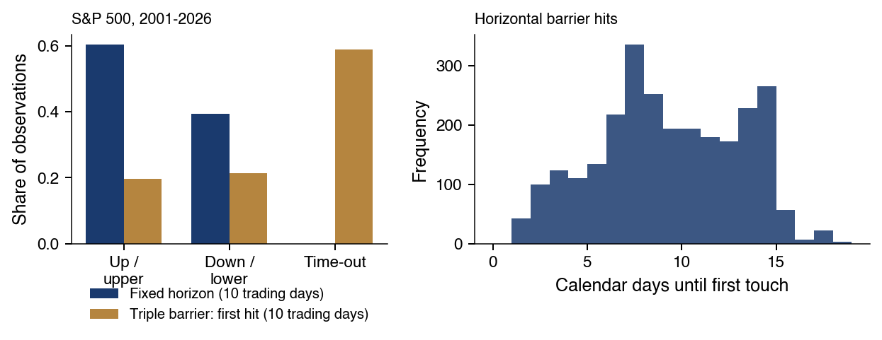
The label in (13.14) has three problems. A constant \(\tau\) ignores time-varying volatility, so the same threshold is a large move in a calm year and a small one in a crisis. The path is ignored: a stop-loss could have been hit before \(t + h\), and the label would still record only the return at the horizon. The classes are unbalanced: for the S&P 500 with \(h = 10\) and \(\tau = 0\), 60.5% of the labels are up and 39.5% down.
In brief
The question of this section
which label reproduces a trader's real decision, with take-profit, stop-loss and a maximum holding period?
Fixed horizon: the label is the sign of the \(h\)-day log return
The triple-barrier label (López de Prado, 2018) starts at an event time \(t_0\), with daily volatility \(\sigma_{t_0}\) and horizon \(h\). The upper barrier, for profit-taking, is reached when \(\log P_t - \log P_{t_0} \ge \pi_u \sigma_{t_0}\sqrt{h}\); the lower barrier, the stop-loss, when the same difference is \(\le -\pi_l \sigma_{t_0}\sqrt{h}\); and the vertical barrier is the date \(t = t_0 + h\). The label is set by the first barrier touched, at time \(t_1\):\(+1\) for the upper barrier, \(-1\) for the lower one, and at the vertical barrier the sign of \(r_{t_0,t_1}\), or 0 under an alternative convention.
The quantity \(\sigma_{t_0}\sqrt{h}\) is the typical \(h\)-day move, and \(\pi_u, \pi_l > 0\) are the barrier widths in units of it. Each label has a span \([t_0, t_1]\), which records the days whose returns it uses; the span is the input of purging in validation.
The daily volatility \(\sigma_{t_0}\) is the square root of an exponentially weighted moving average (EWMA) of squared deviations of daily log returns, with span 50:
where \(\bar r_t\) is the exponentially weighted mean return. A span of 50 gives an effective memory of about two trading months. Volatility-scaled barriers are needed because a fixed threshold would be hit almost daily in 2008 or March 2020 and rarely in calm years.
The chart shows the level of the S&P 500 during the 2022 bear market, with five labelling events. For each event, the dot marks the entry, the green line the upper barrier, the red line the lower barrier and the brown line the horizon; the star marks the first barrier touched, and its colour shows which. The first slider sets the barrier width \(\pi = \pi_u = \pi_l\) in units of \(\sigma\sqrt{h}\), the second the horizon \(h\) in trading days, and the ▶ button widens the barriers step by step.
Question for the room An event first hits the profit barrier on day 5. On day 15, the price is below its entry level. Which label does the page’s implementation assign?
Answer
The event ends on day 5 and receives +1. Subsequent price movements do not change its label. The return sign at the horizon is used only when neither horizontal barrier has already been hit; conflicting signs are not cancelled. On the chart, only the March event reaches the profit barrier; the May, August and November events receive +1 from the return sign at the vertical barrier, and the January event hits the stop-loss (−1).
At \(\pi_u = \pi_l = 1\) and \(h = 15\) days, the January event hits the stop-loss and gets \(-1\), and the March event reaches the profit barrier and gets \(+1\). The other three events end at the vertical barrier, marked by amber stars, above their entry level, so the sign rule labels them \(+1\). Narrower barriers turn more events into horizontal exits; wider barriers send more of them to the vertical barrier.
The five events during the 2022 bear market use \(\pi_u = \pi_l = 1\) and \(h = 15\) days. The chart shows the index level, with green lines for the upper barriers, red lines for the lower barriers and brown lines for the horizons; dots are entries and stars the first barrier touched, coloured by its type.
In January the stop-loss is hit first, and the label is \(-1\). In March the profit-taking barrier is hit first, and the label is \(+1\). The other three events end at the vertical barrier, above their entry level, so the sign rule labels them \(+1\).
A label \(+1\) therefore does not mean that the profit barrier was touched. Under the sign rule, three of the four positive labels in the example come from the vertical barrier. The distribution of exit types over the full sample is shown in Further Topics.
In brief
Five events during the 2022 bear market, \(\pi_u = \pi_l = 1\), \(h = 15\) days
the colour of each star is the barrier touched first
Chart: the index level
green lines: upper barrier, red: lower barrier, brown: horizon
dots: entry, stars: first barrier touched
January: stop-loss hit (\(-1\)); March: profit-taking (\(+1\))
the other three end at the vertical barrier (amber stars) above their entry level
so the sign rule labels them \(+1\)
A label \(+1\) therefore does not mean that the profit barrier was touched
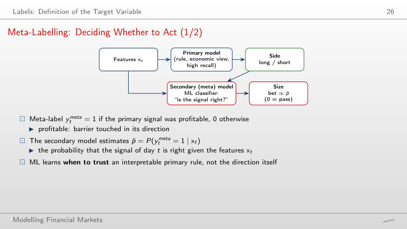
Meta-labelling splits a trading decision into two models. A primary model, which may be a simple rule or an economic view chosen for high recall, uses the features \(\mathbf{x}_t\) to set the side of the trade, long or short. A secondary, or meta, model is an ML classifier that receives the same features and the primary signal and answers a narrower question: is the signal right? Its output sets the size of the bet, proportional to its predicted probability, with zero meaning that the signal is skipped.
The meta-label is \(y^{meta}_t = 1\) if the primary signal was profitable, that is, if the barrier was touched in its direction, and \(0\) otherwise. The secondary model estimates \(\hat p = P(y^{meta}_t = 1 \mid \mathbf{x}_t)\), the probability that the signal of day \(t\) is right given the features.
The division of labour is the point of the method. ML learns when to trust an interpretable primary rule, not the direction of the market itself, which the previous sections showed to be nearly unpredictable.
TP (true positives) counts the profitable signals taken, FP (false positives) the unprofitable signals taken, and FN (false negatives) the profitable signals skipped. Acting on every signal gives recall 1. \(F_1\) is the harmonic mean of precision and recall and lies between 0 and 1.
The example comes from Seminar 13, exercise B11: a crossover of the 20- and 50-day moving averages (MA20/MA50) on Bitcoin, with 1,660 test trades. With the meta filter, precision rises from 0.475 to 0.517, recall falls from 1 to 0.541, and \(F_1\) falls from 0.644 to 0.529. The mean gross log return per trade, before costs, moves from −0.27% to +0.19%.
Meta-labelling raises precision at the cost of recall. With a cost per trade, precision and the return per trade matter, not \(F_1\), which penalises the trades skipped as heavily as the losing trades taken.
In brief
A filter decides which signals to act on; three scores describe it
The label fixes what the model learns. Fixed-horizon labels on the S&P 500 are unbalanced, 60.5% up at \(h = 10\), and ignore the path; triple-barrier labels scale the barriers by volatility and record a span for each label. Meta-labelling uses ML to decide when to act on a primary rule; on the Bitcoin crossover it raises precision from 0.475 to 0.517 and turns the mean gross return per trade from −0.27% to +0.19%.
Validation without Information Leakage
Cross-validation estimates how a model performs on data it has not seen, but only if the training and test sets do not share information. In financial data they usually do: features are serially correlated and labels overlap in time. This section defines leakage, presents purged K-fold CV with an embargo (López de Prado, 2018) and measures, on a target with nothing to predict, how much ordinary shuffled K-fold overstates skill.
Leakage occurs when the training set contains information that is also present in the test set, so that the test score no longer measures performance on genuinely new data. The question of this section is why ordinary \(K\)-fold overstates a model's skill on financial series.
Two properties of financial data create leakage. Features are serially correlated, \(\mathbf{x}_t \approx \mathbf{x}_{t+1}\), because they are built from rolling windows, and labels overlap, \(y_t \approx y_{t+1}\), because consecutive multi-day returns share most of their daily returns. A shuffled \(K\)-fold therefore puts near-identical days on both sides of the boundary. A flexible model, such as RF or GBM, memorises the neighbour and reaches an excellent "out-of-sample" score; tuning on such a leaky CV selects the most overfitted model.
Other sources of leakage are transformations fitted on the full sample, such as scaling, principal component analysis or the choice of \(d\) for FFD. Survivorship bias, data revisions and wrong timestamps add information that was not available at the decision date.
In brief
The question of this section
why does ordinary \(K\)-fold overstate a model's skill on financial series?
Definition (Leakage).
The training set contains information that is also present in the test set
so the test score no longer measures performance on genuinely new data
Serially correlated features (\(\mathbf{x}_t \approx \mathbf{x}_{t+1}\)) and overlapping labels (\(y_t \approx y_{t+1}\))
a shuffled \(K\)-fold puts near-identical days on both sides
A flexible model (RF, GBM) memorises the neighbour \(\Rightarrow\) excellent “out-of-sample” score
tuning on a leaky CV selects the most overfitted model
Other sources of leakage
transformations fitted on the full sample (scaling, principal component analysis, the choice of \(d\) for FFD)
survivorship bias, data revisions, wrong timestamps
Purged \(K\)-fold uses contiguous blocks in time as folds (López de Prado, 2018). Test fold \(k\) holds the observations \(t^{a}_k, \dots, t^{b}_k\), whose labels end at the latest at \(T_k = \max_{i \in \text{test}_k} t_{1,i}\). The training set keeps only the observations that do not touch the test fold:
Purging: it removes the training labels whose span overlaps the span of the test labels.
Embargo: it removes the \(e\) observations that start right after \(T_k\), the end of the last test label, for example 1% of the sample. The embargo is needed because features look back in time, so the observations just after the test block still carry information from it.
The purged CV score is the mean of \(K\) scores, each from a model fitted on \(\mathcal{A}_k\) and evaluated on fold \(k\). With labels of length \(h\), a boundary removes \(h\) observations before the test block and \(h + e\) after it, so an interior fold loses \(2h + e\) observations from training. A 10-observation example is worked out in the Appendix.
The next chart shows five folds in rows, with the observation index on the horizontal axis. Blue marks training observations, red test observations, purple the purged ones and brown the embargo.
Each row of the chart is one split of the sample: the test block in red, the training observations in blue, the observations removed by purging in purple and those removed by the embargo in brown. The three sliders set the number of folds \(K\), the label length \(h\) and the embargo \(e\), all in observations; the ▶ button runs through the settings.
Question for the room In the scheme with 100 observations and 5 folds, keep the embargo at e = 3. If label length increases from h = 4 to h = 6, how many training observations are excluded around the middle fold?
Answer
The number excluded is 2h + e = 15: h = 6 before the block, whose labels end inside the test set, and h + e = 9 after it, i.e. 6 purged and 3 embargoed. The answer 13 updates only the left boundary; 12 omits the embargo. The 20 test observations are not included in this count.
With labels of length \(h\), each interior test block loses \(h\) training observations before it and \(h + e\) after it, \(2h + e\) in all; the first and last folds lose only one side. Raising \(h\) widens the purple bands on both sides of every test block, while raising \(e\) widens only the brown band after it. With few folds the removed observations are a small share of the training set; with many folds they become a large one.
The experiment builds a target with nothing to predict. The price is a pure random walk, the label is the sign of the 20-day forward return, and the 5 features are 20-day rolling means of independent noise. The true accuracy is therefore 50% by construction. A random forest is evaluated with 5 folds under three schemes. The slider sets the common length \(h\) of the labels and of the rolling means, and the charts show the accuracy of each scheme.
Question for the room In the simulation with independent, symmetric increments and noise features, shuffled K-fold gives 69.4%, versus 49.6% with purging and embargo. What explains the difference?
Answer
At h = 20, neighbouring days have overlapping labels and similar features. Shuffling distributes them between training and test. Class imbalance does not explain the difference between evaluations on the same observations, and repeated splitting does not remove this mechanism. Contiguous folds give 50.0%, purging and embargo 49.6%; these values are simulation outcomes, not exact guarantees. With h = 2, shuffled K-fold gives 49.9%; with h = 60 it reaches 84.5%.
Shuffled K-fold reports an accuracy of 69.4%, contiguous K-fold 50.0% and purged K-fold with embargo 49.6%. Shuffling fails because labels overlap and features persist, so the test days have near-duplicates in the training set. Here contiguous folds already remove most of the leak, since only the fold boundaries share returns, and purging cleans those.
A result that looks too good is usually leakage. What the experiment supports is a comparison of procedures on the same data, not a statement about any real predictor.
In brief
Price = pure random walk
label = sign of the 20-day forward return
5 features = 20-day rolling means of independent noise
True accuracy is 50% by construction
Random forest, 5 folds
Shuffled K-fold: 69.4%
contiguous K-fold 50.0%
purged K-fold + embargo 49.6%
Shuffling fails because labels overlap and features persist
here contiguous folds already remove most of the leak: only the fold boundaries share returns, and purging cleans them
Ordinary \(K\)-fold is not always invalid for time series. Bergmeir, Hyndman & Koo (2018) show that it is valid for a purely autoregressive model with serially uncorrelated errors. The conditions under which it fails, and how to check them, are in the Appendix.
Two tasks require different schemes. Model selection, the choice of features, family and tuning, uses purged \(K\)-fold or combinatorial purged CV (CPCV). CPCV tests on many combinations of groups and returns a distribution of Sharpe ratios instead of one number.
Deployment is evaluated by walk-forward (WF): the model is trained on \([0, T_k]\), tested on \((T_k, T_{k+1}]\) and rolled forward, where \(T_k\) is the end of the \(k\)-th training window. Walk-forward is realistic, but it produces a single path with high variance, so it serves the final evaluation and not the choice of the model. Both schemes are compared in the Appendix.
In brief
Ordinary \(K\)-fold is valid for a purely autoregressive model with serially uncorrelated errors (Bergmeir, Hyndman & Koo (2018))
Model selection: purged \(K\)-fold, or combinatorial purged CV (CPCV)
CPCV tests on many combinations of groups and returns a distribution of Sharpe ratios instead of one number
Deployment: walk-forward (WF)
train on \([0, T_k]\), test on \((T_k, T_{k+1}]\), roll forward (\(T_k\): end of the \(k\)-th training window)
realistic, but a single path with high variance: it serves the final evaluation, not the choice (WF and CPCV: Appendix)
Section summary
Shuffled K-fold finds 69.4% accuracy in pure noise, while contiguous and purged folds report 50.0% and 49.6%. Purging removes the training labels that overlap the test span, and the embargo removes the observations right after it, \(2h + e\) observations per interior fold. The case study that follows uses purged 5-fold CV with a 1% embargo for every model.
Case Study: Predicting the S&P 500
The case study applies the toolbox and the validation scheme to one question: can the 5-day direction of the S&P 500 be predicted? Four models are compared on the same purged folds with a naive benchmark, the differences are tested with procedures that respect overlapping labels, and the best model is traded in a walk-forward backtest with costs. A second case study, on the paper of Dong, Li, Rapach & Zhou (2022), asks whether cross-sectional anomalies predict the market return.
Case Study: Can the 5-Day Direction of the S&P 500 Be Predicted?
The data are daily closes of the S&P 500 index and of the VIX from the course data, 2001–2026, with \(n = 6{,}269\) observations. The VIX is the volatility index of the Chicago Board Options Exchange (CBOE), the 30-day implied volatility of S&P 500 options. The S&P 500 is the most liquid equity index and has a long VIX history; if its direction were predictable, arbitrage would be cheap.
The target is the fixed-horizon label with \(h = 5\) and \(\tau = 0\):
equal to 1 if the index is higher 5 days later. Five days correspond to a weekly trading horizon and give about \(6{,}269/5 \approx 1{,}250\) non-overlapping labels. The label span \([t, t+5]\) is used for purging.
Validation is purged 5-fold CV with a 1% embargo, with the same folds for every model. Each fold covers about 5 years, hence at least one crisis episode.
In brief
S&P 500 index and VIX, daily closes of the course data, 2001–2026: \(n = 6{,}269\) observations
the sample starts in October 2001: the first 444 days of 2000–2001 feed the FFD window
VIX: the CBOE (Chicago Board Options Exchange) volatility index, the 30-day implied volatility of S&P 500 options
Why the S&P 500: the most liquid equity index, with a long VIX history
if its direction were predictable, arbitrage would be cheap
Accuracy is the share of days whose direction is predicted correctly. The receiver operating characteristic (ROC) area under the curve (AUC) is the probability that a randomly chosen up day gets a higher predicted probability than a randomly chosen down day. AUC \(= 0.5\) means no skill and AUC \(= 1\) a perfect ranking.
A small example fixes the definition. Let the up days have predicted probabilities 0.7 and 0.4 and the down days 0.5 and 0.2. Of the four (up, down) pairs, three are ranked correctly, all except (0.4, 0.5), so AUC \(= 0.75\). Both metrics are needed: accuracy depends on the 0.5 threshold that turns a probability into a predicted direction, while AUC compares only the ranking of the probabilities.
Two ways of aggregating over folds are used. The fold mean computes the metric in each of the 5 test folds and averages the five values. The pooled metric is computed once on all out-of-fold predictions together, and it is the input of the formal tests.
In brief
Accuracy: share of days whose direction is predicted correctly
Receiver operating characteristic (ROC) area under the curve (AUC)
the probability that a randomly chosen up day gets a higher predicted probability than a randomly chosen down day
AUC \(= 0.5\): no skill; AUC \(= 1\): perfect ranking
Example: up days with probabilities 0.7 and 0.4, down days with 0.5 and 0.2
3 of the 4 pairs are ranked correctly, so AUC \(= 0.75\)
Why both metrics
accuracy depends on the \(0.5\) threshold
AUC compares only the ranking of the probabilities
Fold mean: the metric computed in each of the 5 test folds, then averaged
Pooled: the metric computed once on all out-of-fold predictions together
All 14 features use information up to day \(t\) only. Momentum is the log return over the last \(h\) days, \(\log P_t - \log P_{t-h}\), for \(h \in \{1,5,20,60,120\}\). Realised volatility is the annualised standard deviation (SD) of daily log returns over 20 and 60 days, together with their ratio. The distance to a moving average is \(\log P_t\) minus the mean of \(\log P\) over 50 or 200 days.
The relative strength index, RSI(14), is \(100 - 100/(1+RS)\), where \(RS\) is the smoothed average gain over the average loss over 14 days; it lies between 0 and 100 and is high after rises. The VIX enters through its log level and its 5-day change. The last feature is the FFD log price with \(d = 0.25\), chosen on the full sample; an ablation after the model comparison removes it.
The four models are deliberately conservative. The logit is L2-penalised (ridge) on standardised features. The RF has 400 trees with a minimum leaf size of 100. The GBM is histogram-based, with depth 3, learning rate 0.03 and 200 trees. The MLP has hidden layers of 32 and 16 units and early stopping on a purged chronological validation set. Large leaves and shallow trees limit variance, in line with (13.5).
In brief
Features, information up to day \(t\)
Momentum: \(\log P_t - \log P_{t-h}\)
the log return over the last \(h\) days, \(h \in \{1,5,20,60,120\}\)
Realised volatility
annualised standard deviation (SD) of daily log returns over 20 and 60 days, and their ratio
Distance to moving average
\(\log P_t\) minus the mean of \(\log P\) over 50 or 200 days
RSI(14): \(100 - 100/(1+RS)\)
\(RS\) = smoothed average gain over average loss, 14 days
between 0 and 100, high after rises
VIX: log level and 5-day change
FFD log price, \(d = 0.25\)
chosen on the full sample (ablation after the model comparison)
Models, deliberately conservative
Logit: L2-penalised (Ridge), standardised features
RF: 400 trees, minimum leaf 100
GBM: histogram-based
depth 3, learning rate 0.03, 200 trees
MLP: hidden layers of 32 and 16 units, early stopping on a purged chronological validation set
Large leaves and shallow trees limit variance
A Classifier That Predicts Only the Majority Class (1/2)
The confusion matrix of the L2-penalised logit, from the pooled out-of-fold predictions of purged 5-fold CV with \(n = 6{,}269\), has four cells. TP (true positives) counts the up days predicted up, 3,575; FN (false negatives) the up days predicted down, 65; FP (false positives) the down days predicted up, 2,589; and TN (true negatives) the down days predicted down, 40.
The scores follow from the table. Accuracy is \((TP + TN)/n = 57.7\%\). Precision is \(TP/(TP+FP) = 0.580\), recall \(TP/(TP+FN) = 0.982\), and \(F_1 = 0.729\) by (13.15).
The model predicts "up" on 98.3% of the days. It has essentially learned the rule "always up", and its high recall and \(F_1\) are a consequence of that rule, not of skill.
In brief
Pred. up
Pred. down
Actual up
TP \(=3{,}575\)
FN \(=65\)
Actual down
FP \(=2{,}589\)
TN \(=40\)
L2-penalised logit, \(n = 6{,}269\)
pooled out-of-fold predictions of purged 5-fold CV
The majority baseline comes from the same table. The actual up days are \((3{,}575 + 65)/6{,}269 = 3{,}640/6{,}269 = 58.1\%\) of the sample, which is the accuracy of predicting "up" every day with no model at all. A model with 57.7% accuracy is therefore worse than doing nothing.
The cause is class imbalance. With weak features, the predicted probabilities stay near the base rate 0.58, above the 0.5 threshold, so almost every day is classified "up". The case study keeps the fixed-horizon label on purpose, so that the baseline is transparent; triple-barrier labels change the class balance the classifier sees, as Seminar 13 shows in exercises B1 and B8.
Other baselines are possible: yesterday's direction, a moving-average rule and, for trading, buy-and-hold. Whatever the baseline, a model has value only if it beats it out of sample, after costs, by more than sampling error.
In brief
Majority baseline from the same table
actual up days \((3{,}575 + 65)/6{,}269 = 3{,}640/6{,}269 = 58.1\%\)
the accuracy of predicting “up” every day, with no model at all
A 57.7%-accurate model is worse than doing nothing
The cause is class imbalance
with weak features the predicted probabilities stay near the base rate \(0.58\), above the \(0.5\) threshold
so almost every day is classified “up”
the case study keeps the fixed-horizon label on purpose, so that the baseline is transparent
triple-barrier labels change the class balance the classifier sees (Seminar 13, exercises B1 and B8)
Other baselines: yesterday's direction, a moving-average rule, buy-and-hold for trading
A model has value only if it beats the baseline out of sample
The left chart shows the accuracy of the four models and the right chart their AUC, as means over the 5 purged folds with whiskers of \(\pm 1\) SD across folds. The dashed line in the accuracy chart is the "always up" baseline. The slider sets the probability threshold above which a day is predicted "up", and the lower chart shows the fold-mean accuracy of each model as a function of this threshold; AUC does not depend on it.
Question for the room At threshold 0.5, the logit has 57.7% accuracy. Does this result establish an accuracy advantage over the always-"up" rule?
Answer
No. The always-"up" rule has 58.1%, so the logit is about 0.4 percentage points below the benchmark. Exceeding 50% or ranking ahead of the other three models does not establish superiority over this benchmark. Predicting "up" on 98.3% of days (TP = 3,575, FP = 2,589) indicates proximity to the majority rule; it does not mean the model reproduces that rule exactly. The fold-mean AUCs lie between 0.477 and 0.508.
At the 0.5 threshold the fold-mean accuracies are 57.7% for the logit, 56.3% for the RF, 54.4% for the GBM and 56.6% for the MLP, all below the 58.1% of "always up". The fold-mean AUCs are 0.477, 0.501, 0.507 and 0.508, all close to 0.5. No model beats the baseline.
Lowering the threshold makes the models predict "up" on more days, and their accuracy moves towards that of the baseline; raising it produces more "down" predictions. With AUCs near 0.5, the threshold changes which days are called "up" but cannot add ranking skill. The FFD ablation in Further Topics reaches the same negative conclusion without the FFD log price.
In brief
Fold mean
Logit
RF
GBM
MLP
Accuracy
57.7%
56.3%
54.4%
56.6%
AUC
0.477
0.501
0.507
0.508
Bars: mean over the 5 purged folds; whiskers: \(\pm 1\) SD across folds
\(\hat P\) is the share of days with the correct sign, \(\hat p_y\) and \(\hat p_x\) are the shares of realised and of predicted "up", and \(\hat P^*\) is the share correct expected if the predictions were independent of the outcomes. Under \(H_0\) of independence, \(\widehat{\mathrm{SE}}\) is the standard error of \(\hat P - \hat P^*\), given in the Appendix. A value \(PT > 1.645\) indicates skill at 5% (one-sided), and \(PT < 0\) means fewer hits than chance.
PT assumes independent days, which overlapping 5-day labels violate. The case study therefore also uses the \(t\)-statistic of the slope in \(y_t = a + b\,x_t + u_t\), with \(x_t\) the predicted and \(y_t\) the realised direction, computed with Newey–West standard errors with \(q = 4\) lags (Further Topics); \(b > 0\) means skill.
For the AUC, the DeLong standard error assumes independent days (Appendix). The intervals are therefore computed by a circular block bootstrap (Künsch, 1989) on blocks of \(L = 20\) consecutive days, four times the label length, which keeps the serial dependence within each block.
\(\hat P\): share of days with the correct sign; \(\hat p_y\), \(\hat p_x\): shares of realised and of predicted “up”; \(\hat P^*\): share correct expected if predictions were independent of outcomes
\(H_0\): independence; \(\widehat{\mathrm{SE}}\): standard error of \(\hat P - \hat P^*\) under \(H_0\) (Appendix)
\(PT > 1.645\): skill at 5% (one-sided); \(PT < 0\): fewer hits than chance
PT assumes independent days
with overlapping labels we also use the slope \(t\) in \(y_t = a + b\,x_t + u_t\)
The table uses the pooled out-of-fold predictions. The hit rates \(\hat P\) are slightly below the rates \(\hat P^*\) expected under independence for every model: 0.577 against 0.578 for the logit, 0.563 against 0.570 for the RF, 0.544 against 0.554 for the GBM and 0.566 against 0.569 for the MLP. All PT statistics and all HAC (Heteroskedasticity and Autocorrelation Consistent, standard errors) \(t\)-statistics are negative. The pooled AUCs are 0.480, 0.495, 0.501 and 0.497, and every block-bootstrap 95% confidence interval (CI) contains 0.5; the logit's interval, for example, is \([0.456;\ 0.505]\).
There is therefore no significant positive directional skill. With heteroskedasticity and autocorrelation consistent (HAC) errors at lag 4, no model differs significantly from chance, \(|t| \le 1.67\). The PT statistic, which treats the days as independent, gives \(-2.27\) for the RF, against a HAC \(t\) of \(-1.67\): overlapping labels inflate significance.
The logit gives a second contrast. Its DeLong 95% CI for the AUC is \([0.466;\ 0.494]\) and excludes 0.5, which would read as a model significantly worse than random. The DeLong interval treats days as independent; the block bootstrap does not, and its interval contains 0.5.
The backtest asks whether a trader following the model would have earned more, after costs, than by simply holding the index. The position is \(w_t \in \{0,1\}\): long the S&P 500 if the model's probability of "up" is \(\hat p_t > 0.5\), otherwise cash, decided with information up to \(t\). The decision at the close of day \(t\) is traded at the close of day \(t+1\), so the strategy return is
where \(r_{t+2}\) is the log return of the index from the close of \(t+1\) to that of \(t+2\). The turnover \(|w_t - w_{t-1}|\) is 1 on the days the position changes. The cost is \(c = 5\) basis points (bp), that is, 0.05% per unit traded, a prudent cost for an exchange-traded fund on the S&P 500; \(r - c\) approximates \(\log((1-c)\,e^{r}) = r + \log(1-c)\), the log return after paying the cost.
The exposure \(\bar w = \frac{1}{T}\sum_t w_t\) is the share of the \(T\) days spent invested. Cash earns 0, so interest on cash days is ignored, and both Sharpe ratios use daily log returns with a risk-free rate of 0, annualised with \(\sqrt{252}\).
The model is the GBM, refitted every January over 2010–2026 on all past data, with purging of the labels that overlap the test year. Its FFD log price uses \(d = 0.15\), chosen on data up to 2009 only. The benchmark is buy-and-hold, \(w_t = 1\), with exposure 100% and no turnover.
In brief
The question
would a trader following the model have earned more, after costs, than by simply holding the index?
Position \(w_t \in \{0,1\}\): long the S&P 500 if \(\hat p_t > 0.5\), otherwise cash
decided with information up to \(t\)
\(\hat p_t\): the model's probability of “up”
Strategy return: the index return when invested
minus a cost each time the position changes
the decision at the close of day \(t\) is traded at the close of day \(t+1\)
The chart shows the growth of one dollar invested, on a log scale: buy-and-hold in brown and the GBM strategy in blue. The first slider sets the threshold on the predicted probability above which the strategy is long, the second the cost per change of position in basis points, and the ▶ button moves the threshold.
Question for the room The GBM long/cash strategy has 76% average exposure. Can we treat it as buy-and-hold with constant 76% exposure when comparing Sharpe ratios?
Answer
No. Sharpe-ratio invariance to scaling concerns multiplying every return by the same positive constant. Switching between positions of 0 and 1 is not such a scaling. In this example, trading at the next close, at threshold 0.5 and a 5 bp cost, the strategy has SR (Sharpe Ratio) 0.33 and buy-and-hold 0.66. The difference, −0.33, has p = 0.001 (Ledoit–Wolf HAC test). The FFD log price uses d = 0.15, chosen on data up to 2009 only.
Over 2010–2026, at the 0.5 threshold and a cost of 5 bp, the annualised Sharpe ratio of the strategy is 0.33, against 0.66 for buy-and-hold. The average exposure is 76%. The model stayed mostly long, and its exits from the market, on 24% of the days, lowered the Sharpe ratio rather than raising it.
In brief
2010–2026: strategy Sharpe 0.33 vs. buy-and-hold 0.66 (annualised)
average exposure 76%
The model stayed mostly long
its exits from the market (24% of the days) lowered the Sharpe ratio
The difference between the two Sharpe ratios, \(-0.33\), has \(p = 0.001\) in the Ledoit–Wolf HAC test (Ledoit & Wolf, 2008), discussed in Further Topics. The test requires a finite fourth moment, which Chapter 1 questions. The strategy is significantly worse than buy-and-hold, and there is no evidence of skill. What the result supports is a comparison of procedures: the GBM strategy against buy-and-hold.
The Sharpe ratio of the strategy is sensitive to three design choices. With \(d = 0.25\), chosen on the full sample and hence with information from the test period, it is 0.31. Without the FFD log price it is 0.48. When the trade is executed at the same close as the decision, an idealisation with no execution delay, it is 0.43. None of these variants approaches the 0.66 of buy-and-hold.
The tests of the forecasts themselves against a constant forecast, with the Diebold–Mariano, Clark–West and Giacomini–White tests, are in Further Topics.
In brief
The Sharpe-ratio difference, \(-0.33\), has \(p = 0.001\)
Dong, Li, Rapach & Zhou (2022) ask whether long-short anomaly returns predict next month's market excess return. An anomaly is a portfolio long the stocks with high average returns on a characteristic and short those with low average returns; examples are value (the book-to-market ratio), momentum, accruals and net share issuance. The cross-sectional literature and the predictability of the market return had been studied separately.
The benchmark is hard to beat: Welch & Goyal (2008) show that most published predictors do not beat the historical mean. The paper's data are 100 US anomalies with monthly returns, January 1970 to December 2017. The first out-of-sample forecast has 180 months for 100 predictors, so the regression on all predictors learns noise. The method is therefore shrinkage: the elastic net, forecast combination and dimension reduction.
The main claim is that anomalies have statistically and economically significant out-of-sample predictive power for the market. The proposed explanation is asymmetric limits of arbitrage and persistent correction of overpricing. Overpricing is harder to arbitrage than underpricing, because short selling is costly, so the short leg of the anomalies carries most of the information.
The upper chart cumulates, month by month, the squared errors of the historical-mean forecast minus those of each model, so a rising curve marks months in which the model beats the historical mean and a falling curve months in which it loses. The lower chart shows the \(R^2_{OOS}\) of the single-anomaly forecasts. The slider sets the end of the evaluation period, in December of the chosen year, and the menu chooses the anomalies in the combination: all 15, the 7 factors or the 8 decile spreads.
Question for the room OLS on all 15 anomalies has an R²OOS of −7.41% over 1985–2026. Why does the mean of the 15 univariate forecasts do better, with 0.41%?
Answer
Comb averages univariate forecasts: each univariate slope contributes with weight 1/15. It is not multivariate OLS divided by 15. Combining forecasts can reduce error variance without guaranteeing a gain. Multicollinearity alone does not bias OLS. In this sample, Comb has an R²OOS of 0.41%, versus −7.41% for OLS; the significance of Comb’s gain is sensitive to the HAC lag choice (one-sided Clark–West p 0.045 with 5 lags, 0.063 with 3 lags). In the paper, with 100 anomalies, OLS reaches −2,513.86% and the simple combination 0.89%.
Over 1985–2026 with all 15 anomalies, the simple combination (Comb) ends with an \(R^2_{OOS}\) of 0.41% and the combination elastic net (C-ENet) with 0.08%. Ending the evaluation in 2017 gives the replication's figures for the paper's sample; the full set of numbers and their tests are on the slide "Result and Limits".
where \(r_{t+1}\) is the market excess return (Mkt-RF) in month \(t+1\) and \(x_{i,t}\) the long-short return of anomaly \(i\) in month \(t\). The simple combination (Comb) is the mean of the \(N\) forecasts \(\hat r^{(i)}_{t+1}\). The combination elastic net (C-ENet) applies the elastic net to the regression of \(r_t\) on the \(N\) forecasts, with non-negative coefficients, and forecasts with the mean of the selected forecasts. ENet is the elastic net on all predictors and OLS the regression on all of them.
The paper trains on 1970–1979, validates on 1980–1984 and evaluates out of sample on 1985–2017. The replication uses the Kenneth French Data Library and 15 anomalies instead of 100: SMB (Small Minus Big, size factor), HML (High Minus Low, value factor), RMW (Robust Minus Weak, profitability factor) and CMA (Fama & French, 2015), momentum and short- and long-term reversal, and the extreme-decile spreads for accruals, net issuance, beta, variance, residual variance, E/P, CF (Cornish–Fisher, expansion)/P and D/P.
In the replication, the elastic-net penalty mixes \(\ell_1\) and \(\ell_2\) in equal proportions and is chosen by the small-sample corrected AIC. The out-of-sample period is extended to September 2026.
In brief
Predictive regression of anomaly \(i\), estimated on an expanding window and re-estimated every month
15 anomalies instead of 100: SMB (Small Minus Big, size factor), HML (High Minus Low, value factor), RMW (Robust Minus Weak, profitability factor), CMA (Fama & French (2015)), momentum, short- and long-term reversal
and the extreme-decile spreads for accruals, net issuance, beta, variance, residual variance, E/P, CF/P (cash flow, CF, to price), D/P
elastic-net penalty (\(\ell_1\) and \(\ell_2\) in equal proportions) chosen by the small-sample corrected AIC
Unlike (13.2), the benchmark in (13.21) is the historical mean. The chart cumulates the squared errors of the historical mean minus those of the model, and the curve rises in the months in which the model beats the historical mean.
The paper's figures, from the published version (Table II) for 1985–2017, are 2.81% for C-ENet, 2.03% for ENet, 0.89% for Comb and −2,513.86% for OLS. The replication over 1985–2017 gives 0.35% for Comb, 0.18% for C-ENet, −4.75% for ENet and −6.84% for OLS. Over 1985–2026, Comb reaches 0.41%, with a one-sided Clark–West \(p\)-value of 0.045, and C-ENet 0.08%, with \(p = 0.15\). The Clark–West test (Clark & West, 2007) regresses the adjusted loss difference on a constant with Newey–West errors with \(\lfloor 4(T/100)^{2/9}\rfloor = 5\) lags; with 3, 6 and 12 lags the \(p\)-value of Comb is 0.063, 0.044 and 0.032, and without the HAC correction 0.068. The lag count is fixed by the rule, not chosen by significance, and the test requires a finite fourth moment, which Chapter 1 questions.
After the paper's sample, over 2018–2026, Comb has 0.61% with \(p = 0.12\) and C-ENet −0.23%. What the result supports is the ranking of procedures, forecast combination ahead of the regression on all predictors, not the size of the paper's gains. The main limit is that 15 anomalies do not reproduce the 100: with 15 forecasts, C-ENet selects no forecast in 57% of the months and then uses the historical mean.
In brief
Measure: \(R^2_{OOS}\) against the historical mean \(\bar r_t\), computed up to month \(t-1\) (Campbell & Thompson (2008))
On the S&P 500, no model beats the "always up" baseline of 58.1%: the logit reaches 57.7% by predicting "up" on 98.3% of days, every block-bootstrap AUC interval contains 0.5, and no HAC \(t\)-statistic exceeds 1.67 in absolute value. In the walk-forward backtest the GBM strategy has a Sharpe ratio of 0.33 against 0.66 for buy-and-hold, a difference with \(p = 0.001\). The anomaly replication keeps the ranking of the procedures, forecast combination ahead of OLS, with gains much smaller than the paper's.
Selection and Backtest Overfitting
A researcher who tries many strategies and reports the best one reports a biased estimate, even when every strategy has zero true skill. This section quantifies the bias with the False Strategy Theorem, shows it on a grid of 1,284 trading rules for Bitcoin and corrects it with the probabilistic and deflated Sharpe ratios of Bailey & López de Prado (2012) and Bailey & López de Prado (2014).
The question of the section is how large the best Sharpe ratio among \(N\) trials is when none of them has skill. A researcher who tries \(N\) strategies and reports the best commits selection bias: even if all of them have a true Sharpe ratio of zero, the maximum \(\max_n \widehat{SR}_n\) of the estimated ratios grows with \(N\). In the cross-section of returns, Harvey, Liu & Zhu (2016) conclude that, given hundreds of published factors, a new factor needs \(t > 3\), not 2.
The False Strategy Theorem (Bailey & López de Prado, 2014) gives the size of the maximum. If the estimates \(\widehat{SR}_n\),\(n=1,\dots,N\), are independent and approximately \(N(0, \mathrm{Var}[\widehat{SR}])\), the expected maximum Sharpe ratio is
Here \(\widehat{SR}_n\) is the estimated Sharpe ratio of strategy \(n\),\(\Phi\) the standard Normal distribution function and \(\Phi^{-1}\) its quantile function. \(\mathrm{Var}[\widehat{SR}]\) is the sampling variance of one estimated Sharpe ratio, about \(1/T\) per period for i.i.d. returns, with \(T\) the number of return periods, and \(\gamma_E \approx 0.5772\) is the Euler–Mascheroni constant.
\(SR_0\) is the Sharpe ratio that the luckiest of \(N\) worthless strategies is expected to show. By (13.22) it rises with \(N\), through the Normal quantiles, and with the sampling noise \(\sqrt{\mathrm{Var}[\widehat{SR}]}\), which falls with the length of the sample.
In brief
The question of this section
how large is the best Sharpe ratio among \(N\) trials when none has skill?
A researcher tries \(N\) strategies and reports the best: selection bias
even if all have zero true Sharpe ratio, \(\max_n \widehat{SR}_n\) grows with \(N\)
Harvey, Liu & Zhu (2016): given hundreds of published factors, a new factor needs \(t > 3\), not 2
The left chart shows the best annualised Sharpe ratio on the vertical axis against the number of strategies \(N\) on a log scale. The red line is (13.22), and the dots are Monte Carlo means with \(\pm\) one SD. The strategies have i.i.d. zero-mean returns over 5 years of daily data, so the annualised \(\mathrm{Var}[\widehat{SR}] \approx 1/5\). The slider sets \(N\), the right chart shows the distribution of the best Sharpe ratio over 200 Monte Carlo samples for that \(N\), and the ▶ button raises \(N\) step by step.
Question for the room For 1,000 independent zero-skill strategies, each evaluated on 5 years of i.i.d. daily returns, what is the approximate expected maximum annualised Sharpe ratio?
Answer
About 1.45: the theoretical approximation gives 1.46, and the mean of 200 simulations is 1.43. Zero is the mean for an individual strategy; 0.45 = √(1/5) is its approximate standard deviation. The realised maximum varies across samples. The value rises with N and falls with the sample length.
Trying \(N = 1000\) variants yields a best Sharpe ratio of about 1.45, with no skill at all. The Monte Carlo means lie on the curve of the theorem. The histogram shows that the realised maximum varies from sample to sample around this value, and that it moves to the right as \(N\) grows.
In brief
Strategies with i.i.d. zero-mean returns, 5 years of daily data (annualised \(\Var[\widehat{SR}] \approx 1/5\))
Trying \(N=1000\) variants yields a best Sharpe ratio of \(\approx 1.45\) — with no skill at all
Horizontal axis: number of strategies \(N\) (log scale); vertical axis: best annualised SR
red line: the theorem; dots: Monte Carlo mean \(\pm\) one SD, in line with the theorem
The grid search uses a moving-average (MA) crossover on Bitcoin: the rule is long when the fast MA of the log price exceeds the slow MA by more than a band. The grid has 1,284 configurations of (fast, slow, band). The in-sample (IS) period runs from 16 May 2015 to 2020 and the out-of-sample (OOS) period covers 2021–2026. The tested family, fixed in sample only, consists of the 1,282 rules with non-zero in-sample variance. Three of them stay in cash throughout the OOS period; their OOS Sharpe ratio is undefined and counted as 0. As in the S&P 500 backtest, the decision at the close of day \(t\) is traded at the close of \(t+1\).
The rule selected in sample, with moving averages of 11 and 20 days, has an annualised Sharpe ratio of 2.02 in sample and 0.03 out of sample, both annualised with \(\sqrt{365}\). Over all rules, the Spearman rank correlation between the IS and OOS Sharpe ratios is \(\rho = 0.13\). The median OOS Sharpe ratio is 0.50 for the top 10% in sample and 0.41 for all rules.
The result is consistent with overfitting of the selected rule. A positive Sharpe ratio for the family does not show incremental predictive information, since a trend rule on an asset that rose earns part of the asset's own return; skill against buy-and-hold needs a separate test, the SPA test in Further Topics. What the result supports is a comparison of procedures: a choice made in sample and judged out of sample.
In brief
Moving-average (MA) crossover on Bitcoin
long when the fast MA of the log price exceeds the slow MA by more than a band
1,284 configurations (fast, slow, band)
in sample (IS) 16 May 2015 – 2020, out of sample (OOS) 2021–2026
the tested family, fixed in sample only: the 1,282 rules with non-zero in-sample variance
3 of them stay in cash throughout the OOS period: OOS SR undefined, counted as 0
the decision at the close of day \(t\) is traded at the close of \(t+1\)
Next chart: IS Sharpe ratio on the horizontal axis, OOS Sharpe ratio on the vertical axis
brown points: the top 10% in sample; red star: the selected rule; dotted line: equal SRs
Selected rule (11/20 days): SR\(_{IS}\)2.02\(\to\) SR\(_{OOS}\)0.03 (annualised with \(\sqrt{365}\))
Spearman rank correlation between IS and OOS SR: \(\rho = 0.13\)
Median OOS SR 0.50 for the top 10% in sample vs. 0.41 for all rules
The result is consistent with overfitting of the selected rule
A positive family SR does not show incremental predictive information
skill against buy-and-hold needs a separate test (SPA, in Further Topics)
Type of evidence: comparison of procedures (in-sample choice, judged out of sample)
Each point of the chart is one rule, with its IS Sharpe ratio on the horizontal axis and its OOS Sharpe ratio on the vertical axis. Brown points are the top rules in sample, the red star is the selected rule and the dotted line marks equal Sharpe ratios. The first slider moves the start of the out-of-sample period, on 1 January of the chosen year, and the second sets the share \(q\) of the best rules in sample that are highlighted.
Question for the room Using only May 2015–December 2020, we select the rule with the highest in-sample SR, 2.02. What SR does this rule achieve in 2021–2026?
Answer
The MA 11/20 rule with a 0% band has an out-of-sample SR of 0.03. The values 0.50 and 0.41 describe group medians (the top 10% in-sample rules and all rules), not this rule’s performance. The Spearman rank correlation between in-sample and out-of-sample SR is 0.13. The decline is consistent with overfitting; comparison with buy-and-hold requires a separate evaluation.
With the OOS period starting in 2021 and \(q = 10\%\), the cloud is almost flat: the Spearman correlation between IS and OOS Sharpe ratios is 0.13. The selected rule moves from 2.02 in sample to 0.03 out of sample, and the top 10% in sample have a median OOS Sharpe ratio of 0.50 against 0.41 for all rules.
Two questions precede any correction for selection: how precise an estimated Sharpe ratio is, and how it is compared with a benchmark. The per-period Sharpe ratio of daily log returns, with a risk-free rate of 0, is \(\widehat{SR} = \bar r/\hat\sigma\). The shape of the return distribution enters through the skewness \(\gamma_3 = \mathbb{E}[(r-\mu)^3]/\sigma^3\) and the ordinary kurtosis \(\gamma_4 = \mathbb{E}[(r-\mu)^4]/\sigma^4\), which equals 3 for the Normal distribution, where \(\mu\) and \(\sigma\) are the mean and SD of \(r\).
For i.i.d. returns, the delta method gives the sampling variance (Lo, 2002; Opdyke, 2007)
where \(T\) is the number of returns and \(SR\) the true per-period Sharpe ratio. Negative skewness and fat tails widen the uncertainty. For the Normal distribution, \(\gamma_3 = 0\) and \(\gamma_4 = 3\), and (13.23) reduces to \((1 + \frac12 SR^2)/T\).
The formula requires a finite fourth moment, which Chapter 1 questions. Annualisation with \(\sqrt{A}\), where \(A\) is the number of return periods per year, also assumes zero autocorrelation; the correction is in Further Topics.
In brief
The question
how precise is an estimated Sharpe ratio?
how do we compare it with a benchmark?
Per-period Sharpe ratio of daily log returns, risk-free rate 0: \(\widehat{SR} = \bar r/\hat\sigma\)
Shape of the distribution, with \(\mu\), \(\sigma\) the mean and SD of \(r\)
skewness \(\gamma_3 = \E[(r-\mu)^3]/\sigma^3\)
ordinary kurtosis \(\gamma_4 = \E[(r-\mu)^4]/\sigma^4\) (\(3\) for the Normal distribution)
Sampling variance of \(\widehat{SR}\), i.i.d. returns, delta method (Lo (2002); Opdyke (2007)):
The probabilistic Sharpe ratio (PSR) of Bailey & López de Prado (2012) is called by its authors the probability that the true Sharpe ratio exceeds a benchmark \(SR^*\). Formally it is \(\Phi\) of a \(z\)-statistic whose denominator is the standard deviation from (13.23):
\(SR^*\) is the benchmark, for example 0 or the expected maximum \(SR_0\) of (13.22), and \(\hat\gamma_3\),\(\hat\gamma_4\) are the sample skewness and kurtosis.
The reading follows from the construction: \(\widehat{PSR} = 1 - p\), where \(p\) is the one-sided \(p\)-value of \(H_0: SR \le SR^*\). A value \(\widehat{PSR} > 0.95\) therefore means rejecting \(H_0\) at 5%, under i.i.d. returns and the delta-method approximation. It is not a 95% probability for the true Sharpe ratio, which is a fixed number in this frequentist setting.
The deflated Sharpe ratio (DSR) (Bailey & López de Prado, 2014) is the PSR with the benchmark set to the expected maximum of the False Strategy Theorem, \(DSR = \widehat{PSR}(SR_0)\), with \(SR_0\) computed from the variance \(\mathrm{Var}[\widehat{SR}_n]\) of the trials. It corrects at once for selection over \(N\) trials, for non-Normality and for the length of the sample, so \(N\) must always be reported. A value \(DSR \le 0.95\) means insufficient evidence at the chosen threshold, not proof that the strategy has no skill.
The worked example is the best in-sample Bitcoin rule, with \(T = 2{,}057\) days. Its Sharpe ratio is \(\widehat{SR} = 0.1055\) a day, 2.02 annualised, with \(\hat\gamma_3 = 0.16\) and \(\hat\gamma_4 = 12.23\);\(\hat\gamma_4\) and the DSR require a finite fourth moment, which Chapter 1 questions. The denominator of (13.24) is \(\sqrt{1 - 0.16\cdot 0.1055 + \frac{12.23-1}{4}\cdot 0.1055^2} = 1.007\), and the family has \(N = 1{,}282\) trials. The argument of \(\Phi\) is \(z = (\widehat{SR} - SR_0)\sqrt{T-1}/1.007\).
The verdict depends on how \(\mathrm{Var}[\widehat{SR}_n]\) is measured. Taken from the observed dispersion of the 1,282 trial Sharpe ratios, the SD is 0.0109, \(SR_0 = 0.036\) a day, \(z = 3.11\) and \(DSR = 0.999\); this dispersion includes the correlation between rules. Treating the rules as independent, with \(\mathrm{Var} = 1/T\), the SD is 0.0220, \(SR_0 = 0.073\),\(z = 1.45\) and \(DSR = 0.926\), the conservative variant. The out-of-sample Sharpe ratio of 0.03 sides with the conservative value; the choice between the two is discussed in Further Topics.
With 1,000 zero-skill strategies over 5 years of daily data, the expected best Sharpe ratio is about 1.45. On the Bitcoin grid, the rule selected in sample falls from a Sharpe ratio of 2.02 to 0.03 out of sample, and the Spearman correlation between IS and OOS ratios is 0.13. The DSR of that rule is 0.999 or 0.926, depending on whether the variance of the trials is taken from their dispersion or set to \(1/T\); only the second, conservative value agrees with the out-of-sample result.
Machine Learning for Inference
Prediction and inference have different targets. A model may predict well while giving a biased estimate of the effect of one variable, and a variable chosen by the LASSO is not thereby significant. This section presents two methods that use ML for the nuisance part of a model and keep valid inference on a parameter of interest: post-double selection (Belloni, Chernozhukov & Hansen, 2014) and double/debiased machine learning (Chernozhukov et al., 2018). A worked example asks whether the VIX predicts S&P 500 returns.
Inference after Variable Selection: Post-Double Selection (1/2)
The question of the section is how to obtain a valid confidence interval for the effect of one variable after ML has chosen the controls. The LASSO path answers "which feature enters first", not "which feature matters", and OLS \(t\)-statistics computed after a LASSO ignore the selection step. A control that is correlated with the regressor of interest \(d_t\) but only weakly with the outcome \(y_t\) gets dropped, and its effect moves into the coefficient of \(d_t\): the omitted-variable bias.
The framework is the partially linear model, in which the effect of \(d_t\) is linear and the controls enter through unknown functions:
\(y_t\) is the outcome, \(d_t\) the regressor of interest and \(\theta\) its effect, the parameter to estimate. \(\mathbf{x}_t\) holds the \(p\) controls, \(g\) is their effect on \(y_t\),\(m\) describes how they predict \(d_t\), and \(\varepsilon_t\),\(v_t\) are errors. The model is approximately sparse when a few controls explain most of \(g\) and \(m\).
In brief
The question of this section
how do we get a valid confidence interval for the effect of one variable after ML has chosen the controls?
The LASSO path answers “which feature enters first”, not “which feature matters”
OLS \(t\)-statistics after LASSO ignore the selection step
A control correlated with the regressor of interest \(d_t\) but only weakly with \(y_t\) gets dropped
its effect moves into the coefficient of \(d_t\) (omitted-variable bias)
Partially linear model: the effect of \(d_t\) is linear
A LASSO of \(y_t\) on \(\mathbf{x}_t\), which selects the set \(\hat S_y\).
A LASSO of \(d_t\) on \(\mathbf{x}_t\), which selects \(\hat S_d\).
An OLS regression of \(y_t\) on \(d_t\) and on the controls kept by either LASSO, \(\mathbf{x}_{\hat S_y \cup \hat S_d}\), with a robust standard error.
The second step is what makes inference valid. A control is missed only if it matters for neither equation of (13.25): if it is weakly related to \(y_t\) but strongly to \(d_t\), the LASSO of \(d_t\) keeps it. The bias from the controls that are still omitted is then of second order.
The method is valid under independent sampling and sparsity. With HAC standard errors it is an approximation for time series. The penalty level and the formal conditions are in the Appendix.
Double/debiased machine learning (DML) (Chernozhukov et al., 2018) residualises both variables with any learner, the LASSO, a random forest or boosting, and then regresses residual on residual:
\(\hat\ell(\mathbf{x}) = \hat{\mathbb{E}}[y \mid \mathbf{x}]\) is the ML prediction of \(y_t\) from the controls and \(\hat m(\mathbf{x})\) the ML prediction of \(d_t\). The residuals \(\tilde y_t\) and \(\tilde v_t\) are the parts of \(y_t\) and \(d_t\) that the controls do not explain, and \(\hat\theta\) is the OLS slope of \(\tilde y_t\) on \(\tilde v_t\).
The estimator solves the sample version of the Neyman-orthogonal score \(\psi = (\tilde y - \theta \tilde v)\,\tilde v\), whose mean is zero at the true \(\theta\). Orthogonality means that first-order errors in \(\hat\ell\) and \(\hat m\) do not bias \(\hat\theta\); the rate conditions are in the Appendix. Cross-fitting fits \(\hat\ell\) and \(\hat m\) on \(K-1\) folds, residualises the held-out fold and repeats over the folds, which removes the bias from overfitting each observation's own value.
The published theory assumes independent sampling. With overlapping 5-day labels, the chapter uses contiguous folds purged by 5 days around the test fold, and HAC standard errors. This is an adaptation to serial dependence outside the published theory.
\(\hat\ell(\mathbf{x}) = \hat\E[y \mid \mathbf{x}]\): ML prediction of \(y_t\) from the controls; \(\hat m(\mathbf{x})\): ML prediction of \(d_t\)
\(\tilde y_t\), \(\tilde v_t\): the parts of \(y_t\) and \(d_t\) the controls do not explain; \(\hat\theta\): OLS slope of \(\tilde y_t\) on \(\tilde v_t\)
The question is whether the level of the VIX predicts the S&P 500 return over the next 5 days, given a large set of controls. The outcome \(y_t\) is the 5-day forward log return in basis points. The regressor of interest \(d_t\) is the log VIX, standardised, with 1 SD \(= 0.356\).
There are 90 controls: 12 technical features, their squares and their pairwise products. The sample has \(n = 6{,}269\) days, and the standard errors are HAC with 4 lags.
The single LASSO drops the VIX and every control. It reports "no effect", with no standard error. Double selection keeps \(|\hat S_y| = 0\) controls in the \(y_t\) equation and \(|\hat S_d| = 15\) in the \(d_t\) equation, where \(|\cdot|\) is the number of elements: none of the controls predicts the return, while 15 of them predict the VIX.
In brief
The question
does the VIX level predict the S&P 500 return over the next 5 days, given a large set of controls?
\(y_t\): 5-day forward log return, in basis points (bp)
\(d_t\): log VIX, standardised (1 SD \(= 0.356\))
90 controls: 12 technical features, their squares and pairwise products
\(n = 6{,}269\) days; HAC errors with 4 lags
The single LASSO drops the VIX and every control
“no effect”, with no standard error
Double selection keeps \(|\hat S_y| = 0\) controls in the \(y_t\) equation and \(|\hat S_d| = 15\) in the \(d_t\) equation
\(|\cdot|\): number of elements
Next chart: one estimator per row
the dot is the estimate of \(\theta\) (bp per week per SD of log VIX)
the bar its 95% HAC CI, the dashed line no effect
Worked Example: Does the VIX Predict S&P 500 Returns? (2/3)
The chart has one estimator per row. The dot is the estimate of \(\theta\), in basis points per week per SD of log VIX, the bar is its 95% HAC confidence interval and the dashed line marks no effect. The slider sets the number of Newey–West lags of the HAC standard errors, and the ▶ button raises it step by step.
Question for the room OLS on log VIX alone gives 7.5 bp, with interval [−10.3, 25.2]. Why is the double-selection interval almost twice as wide?
Answer
With 4 HAC lags, the double-selection interval, [−22.1, 40.8] bp, is about 1.8 times wider. The 15 controls selected for log VIX reduce its remaining variation after adjustment, which can increase the standard error. The methods use the same sample, and both intervals use HAC correction. Coefficient magnitude does not proportionally determine interval width. The [−22.1, 40.8] bp interval does not distinguish the predictive coefficient from zero at the 5% level.
With 4 lags, OLS with log VIX only gives 7.5 with interval \([-10.3;\ 25.2]\), and double selection gives the interval \([-22.1;\ 40.8]\). OLS with all 90 controls, double selection and DML give point estimates of −0.7, 9.4, 4.8 (LASSO) and −11.7 (random forests), all with intervals about twice as wide as the simple OLS interval. The honest intervals contain zero.
Double selection gives a 95% confidence interval for \(\theta\) of \([-22.1;\ 40.8]\) basis points per week per SD of log VIX. OLS with log VIX only gives 7.5, with interval \([-10.3;\ 25.2]\). OLS with all 90 controls, double selection and DML give \(-0.7\),\(9.4\),\(4.8\) (LASSO) and \(-11.7\) (random forests), all with intervals about twice as wide.
The wider intervals have a reason. The controls that predict \(d_t\) absorb part of the variation of the log VIX, and less own variation in \(d_t\) means a wider interval. This is the price of protection against omitted-variable bias. The sign change under DML with random forests is noise: every point estimate lies inside the double-selection and DML intervals.
The honest intervals contain zero and large effects of both signs, so the data cannot decide. What the result supports is an association: the model is a predictive regression, and even a non-zero \(\theta\) would not show that the VIX causes returns.
In brief
Double selection: 95% CI for \(\theta\)\([-22.1;\ 40.8]\)
in bp per week per SD of log VIX
OLS with log VIX only: \(7.5\)\([-10.3;\ 25.2]\)
OLS with all 90 controls, double selection and DML (Double/Debiased Machine Learning) give \(-0.7\), \(9.4\), \(4.8\) (LASSO) and \(-11.7\) (random forests)
all with intervals about twice as wide
Controls that predict \(d_t\) absorb part of the variation of log VIX
less own variation in \(d_t\) means a wider interval
the price of protection against omitted-variable bias
The sign change under DML-RF (DML with random forests) is noise
every point estimate lies inside the double-selection and DML intervals
Honest intervals contain zero and large effects of both signs
the data cannot decide
Type of evidence: association (the variables move together; this does not prove causation)
a predictive regression: even a non-zero \(\theta\) would not show that the VIX causes returns
The LASSO path and the importance of a feature are not evidence of an effect. Post-double selection and DML give valid intervals for one parameter after ML has handled the controls. For the VIX and the 5-day S&P 500 return, every interval contains zero, and the double-selection interval, \([-22.1;\ 40.8]\) bp per week per SD, is about twice as wide as that of simple OLS.
Current Research: Structural and Flexible Models
The frontier of ML in asset pricing divides on the role of model complexity. One line of work argues that heavily over-parameterised models can still forecast well; critical readings trace the gains to simple strategies or to hard-to-arbitrage stocks. The case study of Chen, Pelger & Zhu (2024) takes a third route: it imposes economic structure, the no-arbitrage condition, on a deep network.
The Virtue of Complexity, and a Critical Reading [deeper]
Kelly, Malamud & Zhou (2024) fit ridge regressions on \(P\) random Fourier features of a few predictors, in rolling windows as short as \(T = 12\) months, with \(P\) in the thousands. Random Fourier features are sines and cosines of random linear combinations of the predictors. Their theory shows that with \(P > T\) the minimum-norm solution, the exact fit with the smallest \(\|\boldsymbol\beta\|_2\), shrinks implicitly, the phenomenon called "double descent". The \(R^2_{OOS}\) may be negative while the Sharpe ratio of market timing rises with complexity, so complexity is not automatically overfitting.
Nagel (2025) gives a critical reading. For \(P \gg T\) the forecast is a similarity-weighted average of the \(T\) training returns. In short windows similarity is mostly recency, so the method becomes a volatility-timed momentum strategy, which loses on artificial data with reversals.
Avramov, Cheng & Metzker (2023) find that the profits of deep-learning signals come from hard-to-arbitrage stocks: excluding microcaps, distressed firms or high-volatility episodes attenuates them, and costs erode them further. Chen, Pelger & Zhu (2024) impose economic structure instead, using the no-arbitrage moment conditions as the loss of a deep network. A survey of the field is Kelly & Xiu (2023), and a textbook is Dixon, Halperin & Bilokon (2020).
rolling windows as short as \(T = 12\) months, \(P\) in the thousands
random Fourier features: \(\sin\) and \(\cos\) of random linear combinations of the predictors
theory: with \(P > T\) the minimum-norm solution (the exact fit with the smallest \(\|\bm\beta\|_2\)) shrinks implicitly (“double descent”)
\(R^2_{OOS}\) may be negative while the Sharpe ratio of market timing rises with complexity; complexity is not automatically overfitting
Nagel (2025): for \(P \gg T\) the forecast is a similarity-weighted average of the \(T\) training returns
in short windows similarity is mostly recency, so the method becomes a volatility-timed momentum strategy, which loses on artificial data with reversals
Chen, Pelger & Zhu (2024) estimate the stochastic discount factor (SDF) \(M_{t+1}\) that prices all individual US stocks, conditioning on 46 firm characteristics and on the history of 178 macroeconomic series. Under no arbitrage, the SDF prices every excess return (Section I.A, eq. 1 of the paper):
\(R^e_{t+1,i}\) is the excess return of stock \(i\) over the Treasury bill from month \(t\) to \(t+1\), and \(R^e_{t+1}\) the vector of all stocks. \(E_t\) is the expectation given the information at \(t\), and \(\omega_t\) are portfolio weights, a function of the characteristics and of the macroeconomic states.
The portfolio \(F_{t+1} = \omega_t^\top R^e_{t+1}\), the SDF portfolio, is the conditional tangency portfolio, the portfolio with the highest conditional Sharpe ratio. Condition (13.27) implies the beta representation
\[E_t[R^e_{t+1,i}] = \beta_{t,i}\,E_t[F_{t+1}],\]
(13.28)
where \(\beta_{t,i}\) is the loading of stock \(i\) on \(F\). A stock's expected excess return is its loading times the premium of \(F\); the derivation is in Further Topics.
In brief
Chen, Pelger & Zhu (2024): estimate the stochastic discount factor (SDF) \(M_{t+1}\) that prices all individual US stocks
conditioning on 46 firm characteristics and on the history of 178 macroeconomic series
No arbitrage: the SDF prices every excess return (Section I.A, eq. 1)
\(\beta_{t,i}\): loading of stock \(i\) on \(F\); a stock's expected excess return is its loading times the premium of \(F\) (derivation in Further Topics)
The left chart shows monthly out-of-sample Sharpe ratios of the SDF portfolio. Blue bars are the paper's figures for 1992–2016; red bars are the Fama–French three- and five-factor tangency portfolios (FF3, FF5) computed on the Kenneth French factors, with weights \(w \propto \hat\Sigma^{-1}\hat\mu\), where \(\hat\mu\) and \(\hat\Sigma\) are the sample mean vector and covariance matrix of the factor returns. The right chart shows these weights. The slider sets the last year of the period on which the weights are estimated, and the menu the test period: 1992–2016, 2017–2026 or 1992–2026.
Question for the room With FF5 weights estimated on 1967–1986 and then held fixed, what is the monthly Sharpe ratio over the 1992–2016 test period?
Answer
FF5 has a monthly SR of 0.22, with an approximate 95% interval of [0.11, 0.34]. The page uses standard error √((1 + SR²/2)/T), under an i.i.d. Normal approximation. The values 0.75 and 0.15 belong to the paper’s GAN (Generative Adversarial Network) and the replication’s market benchmark, respectively. In the paper, EN achieves 0.50 and FFN (FeedForward Network) 0.44: the regularised linear model outperforms this forecasting network in the reported comparison, without establishing a universal rule about structure and flexibility.
With weights estimated on 1967–1986 and the test period 1992–2016, the replicated tangency portfolios have monthly Sharpe ratios of 0.22 for FF5 and 0.20 for FF3, next to the paper's 0.22 and 0.19. Switching the test period to 2017–2026 lowers them to 0.06 and 0.03.
The paper's figures, from the published version, are monthly out-of-sample Sharpe ratios over 1992–2016. The full model, labelled GAN (generative adversarial network), reaches 0.75; the elastic-net linear SDF (EN) 0.50; the forecasting feedforward network (FFN) 0.44; and the unregularised linear SDF (LS) 0.42 (Table I). The Fama–French tangency portfolios reach 0.22 for FF5 and 0.19 for FF3 (Table A.VI). The regularised no-arbitrage linear model already beats the forecasting network.
The replication computes the FF3 and FF5 tangency portfolios with weights fixed on 1967–1986. FF5 has 0.22, with 95% interval \([0.11;\ 0.34]\), and FF3 0.20, with interval \([0.08;\ 0.31]\); the standard error is 0.058 (Lo, 2002) and requires a finite fourth moment, which Chapter 1 questions.
What the result supports is a comparison of procedures, the out-of-sample Sharpe ratios of the models. After 2016, the same fixed weights give a monthly Sharpe ratio of 0.06 for FF5 and 0.03 for FF3, as shown in Further Topics.
In brief
Blue: the paper's figures (published version), monthly out-of-sample SR 1992–2016
GAN (the paper’s generative adversarial network) \(0.75\), EN (linear SDF with elastic net) \(0.50\), FFN (the feedforward forecasting network) \(0.44\), LS (unregularised linear SDF) \(0.42\) (Table I)
Complexity alone does not settle the question: the virtue-of-complexity result has a critical reading as volatility-timed momentum, and deep-learning profits concentrate in hard-to-arbitrage stocks. Imposing the no-arbitrage condition gives the GAN of Chen, Pelger & Zhu (2024) a monthly out-of-sample Sharpe ratio of 0.75 over 1992–2016, against 0.22 for FF5. The public-data benchmarks replicate, and their Sharpe ratios fall to 0.06 and 0.03 after 2016.
AI for Scientific Discovery
Artificial intelligence (AI) assistants can propose features, write code and draft papers at a scale that makes the number of trials hard to count. This section states the open question, describes the discovery loop and the checks that remain with the researcher, and runs a mini-case in which an assistant's proposal produces 102 tests.
An Open Question: Discovery or Data Mining at Scale?
Chen, Lopez-Lira & Zimmermann (2022) mine 29,000 accounting ratios for \(t > 2\). The mined signals give cross-sectional predictability similar to that of peer-reviewed predictors, and for both groups about half of the predictability remains after the original samples. Novy-Marx & Velikov (2025) go further: a pipeline built on a large language model (LLM) mines over 30,000 signals, keeps 96 that pass a fixed protocol and writes hundreds of complete papers, with invented motivations and some imagined citations. This is hypothesising after the results are known (HARKing) at scale.
The open question is what the number of trials is when a machine proposes the features, the model and the story, and what then separates a discovery from the best of many draws. The discovery loop gives a structure: literature, competing hypotheses, data and code, robustness fixed in advance, a referee-style critique, and a report of every test. Reusable prompts for each step are in the Appendix.
Some checks remain with the human. Every reference must resolve, through its digital object identifier (DOI) or arXiv identifier. Every trial is logged, so that \(M\) in the correction for multiple testing counts them all. Correlated tests get a common yardstick, such as a placebo or a joint bootstrap of the scores. Transformations are fitted inside the training fold.
The mini-case starts from a typical assistant proposal: "add more indicators", namely momentum, moving-average distances, volatility ratios, the RSI and VIX changes over several windows. The result is 34 features times 3 horizons of 1, 5 and 20 days, that is, 102 predictive regressions on 2001–2015 with Newey–West \(t\)-statistics. Only targets whose window ends by 31 December 2015 are used, so the last 1, 5 and 20 days are dropped at the boundary. Regression \(j\) is \(r_{t,t+h} = \alpha_j + \beta_j x_{j,t} + e_t\), with \(x_{j,t}\) feature \(j\) and \(r_{t,t+h}\) the next \(h\)-day return, and its null hypothesis is \(H_{0,j}: \beta_j = 0\).
The \(M = 102\)\(p\)-values are ordered, \(p_{(1)} \le \dots \le p_{(M)}\), and three corrections are applied:
The Holm procedure rejects while \(p_{(j)} \le 0.05/(M - j + 1)\) and controls the family-wise error rate (FWER), the probability of at least one false rejection.
The Benjamini–Hochberg (BH) procedure (Benjamini & Hochberg, 1995) rejects the \(j\) smallest \(p\)-values for the largest \(j\) with \(p_{(j)} \le j\,q/M\). It controls the false discovery rate (FDR) at \(q\), the expected share of false rejections among all rejections.
A shift placebo, the 95% quantile of \(\max_j |t_j|\) when the target is shifted circularly in time. The shift keeps the correlation between the features, but it also changes their link with conditional volatility, so the placebo is a heuristic yardstick, not an exact test.
In brief
A typical assistant proposal: “add more indicators”
“momentum, moving-average distances, volatility ratios, RSI and VIX changes over several windows”
At \(|t| > 1.96\), 22 of the 102 regressions are significant, against 5.1 expected under the global null at 5%. Holm at a FWER of 5% keeps none, BH at an FDR of 10% keeps 13, and the threshold \(|t| > 3\) of Harvey, Liu & Zhu (2016) keeps 4. The shift placebo, with 500 circular shifts of the target, gives a 95% quantile of \(\max_j |t_j|\) of 3.32. One predictor exceeds it: the 1-day return as a predictor of the next day's return, with \(t = -3.38\), the short-term reversal, a known effect.
The holdout period, 2016–2026, tests the 22 survivors. Three of them keep their sign with \(|t| > 1.96\); all three are variants of the reversal, and the VIX-based "finds" fail. With Holm at 5% over the 22 checks none passes: the smallest \(p\)-value is 0.019, against a threshold of \(0.05/22 = 0.0023\).
BH needs independence or positive dependence of the \(p\)-values of the true nulls, which correlated predictors do not ensure. What the result supports is an association: short-term reversal is a predictive regularity, not an identified mechanism.
In brief
\(|t| > 1.96\): 22 of 102, against 5.1 expected under the global null at 5%
The project asks whether an AI-assisted feature search can find a predictor of index returns, for the S&P 500, for BET, the benchmark index of the Bucharest Stock Exchange, or for Bitcoin. The predictor must survive a pre-registered correction and a holdout, and it must go beyond short-term reversal.
The S&P 500 and Bitcoin are in the course data; BET is not. A team that chooses BET names the source, for example the Bucharest Stock Exchange, freezes the sample, and logs the download date, \(n\) and the first and last close.
The deliverables are a feature list fixed before the data are touched, all tests with Holm, BH and the max-\(|t|\) null, a separate holdout, and the DSR and PBO for any strategy built on the survivors. Each prompt that shaped a decision is logged in `AI_USE.md`, and each invented reference, leak or undercounted trial in `AI_ERRORS.md`, with the test that caught it; templates are provided.
In brief
Questions
can an AI-assisted feature search find a predictor of index returns (S&P 500, BET – the Bucharest Stock Exchange benchmark index, Bitcoin)?
does it survive a pre-registered correction and a holdout?
does it go beyond short-term reversal?
Data: S&P 500 and Bitcoin are in the course data; BET is not
a team that chooses BET names the source (e.g. the Bucharest Stock Exchange) and freezes the sample
it logs the download date, \(n\) and the first and last close
Deliverables
a feature list fixed before the data are touched
all tests with Holm, BH and the max-\(|t|\) null
a separate holdout
DSR and PBO for any strategy built on the survivors
Each invented reference, leak or undercounted trial in AI_ERRORS.md, with the test that caught it
Section summary
Of 102 tests proposed by an assistant, 22 pass \(|t| > 1.96\), none passes Holm, and only the known short-term reversal exceeds the placebo quantile of 3.32; in the holdout, the three nominal replications are reversal variants and none passes Holm. The number of trials is the quantity an AI-assisted search makes hardest to count, and every correction depends on it.
Conclusions
The chapter applied ML to the direction of the S&P 500 and to a grid of Bitcoin trading rules, with validation and tests designed for serially dependent data. The conclusions concern the process more than the algorithms: how features, labels, validation and selection can produce apparent skill, and which tests remove it.
Four empirical lessons stand out. An ADF rejection is not stationarity: truncated FFD of the S&P 500 log price stays \(I(1)\), and memory should be estimated directly, with the local Whittle estimator. Shuffled \(K\)-fold "finds" skill in pure noise, 69.4% accuracy on a target with none.
On the S&P 500, no model beats "always up", whether judged by the PT test or, in Further Topics, by the DM and Giacomini–White (GW) tests. The best of many backtests must be deflated or bootstrapped: on the Bitcoin grid, the best in-sample rule keeps nothing out of sample.
The next chapters continue the topic. Chapter 14 treats deep learning and time-series foundation models, and Chapter 15 large language models and sentiment.
In brief
Four empirical lessons
An ADF rejection is not stationarity
truncated FFD of the S&P 500 log price stays \(I(1)\)
estimate memory directly with local Whittle
Shuffled \(K\)-fold “finds” skill in pure noise
On the S&P 500 no model beats “always up” (PT, DM, GW)
The best of many backtests must be deflated or bootstrapped
on the Bitcoin grid the best in-sample rule keeps nothing out of sample
The checklist collects the conditions under which a predictive claim can be taken seriously. Data are point-in-time, and every transformation is fitted on the training folds only. Labels are scaled by volatility and their spans are recorded. Model selection uses purged \(K\)-fold or CPCV with an embargo, and the final test is a walk-forward.
The evaluation includes a naive baseline, the PT test, the DM, Clark–West (CW) or GW tests, and block-bootstrap intervals. Costs are included and every trial is logged. The selected strategy is assessed with the DSR, the SPA test and the PBO.
The last item separates prediction from inference: "selected" or "important" is not "significant", and inference on an effect requires double selection or DML.
In brief
Point-in-time data; transformations fitted on training folds only
Volatility-scaled labels with recorded spans
Purged \(K\)-fold or CPCV with embargo for selection; walk-forward for the final test
A naive baseline; PT, DM / CW (Clark–West, test for nested models) / GW and block-bootstrap intervals
Costs included and every trial logged
DSR, SPA and PBO for the selected strategy
“Selected” or “important” is not “significant”: double selection or DML for inference
The questions return to the chapter's main numbers: the logit's 57.7% against the 58.1% baseline, the correlation of 0.98 between the FFD series and the log price, the 69.4% of shuffled K-fold against 49.6% with purging, the growth of \(SR_0\) with \(N\), the two DSR values of the best Bitcoin rule, the two AUC intervals of the logit and the question that double selection answers about the VIX. Each answer rests on a slide of the corresponding section.
In brief
Why does the logit with 57.7% accuracy show no skill when 58.1% of the days are “up”?
What does a correlation of 0.98 between the FFD series (\(d = 0.25\)) and the log price say about an ADF rejection?
Why does shuffled \(K\)-fold report 69.4% on a target with nothing to predict, while purged \(K\)-fold with embargo reports 49.6%?
How does \(SR_0\), the expected maximum of \(N\) zero-skill strategies, change when \(N\) rises from 10 to 1,000?
Why does the best Bitcoin rule, with an in-sample SR of 2.02, get a DSR of 0.999 or 0.926 depending on the variance used?
Why do the DeLong interval for the AUC, \([0.466;\ 0.494]\), and the block-bootstrap interval, \([0.456;\ 0.505]\), lead to different conclusions?
Which question about the VIX does double selection answer that the LASSO path does not?
For the 5-day direction of the S&P 500 the choice is buy-and-hold, not the GBM strategy: in the 2010–2026 walk-forward, the Sharpe ratio is 0.66 for buy-and-hold and 0.33 for the GBM. For any model, selection uses purged CV with an embargo, and the final evaluation a walk-forward.
The choice holds under three conditions. The directional signal stays weak, so that no model beats the "always up" benchmark of 58.1%. Each change of position costs 5 bp. Every trial is logged and the number of trials \(N\) is reported.
The choice would be dropped for a model that beats buy-and-hold out of sample, after costs, with a PT statistic above 1.645, a block-bootstrap AUC interval entirely above 0.5 and a DSR above 0.95 under the conservative variance \(1/T\). The best Bitcoin rule, for comparison, has a DSR of 0.926.
In brief
What I choose
for the 5-day direction of the S&P 500: buy-and-hold, not the GBM strategy
in the 2010–2026 walk-forward, the Sharpe ratio is 0.66 for buy-and-hold and 0.33 for GBM
for any model: purged CV with embargo for selection, walk-forward for the final evaluation
Under which conditions
the directional signal stays weak: no model beats the “always up” benchmark of 58.1%
each change of position costs 5 bp
every trial is logged and the number of trials \(N\) is reported
What result would make me drop it
a model that beats buy-and-hold out of sample, after costs
with a PT statistic above 1.645
with a block-bootstrap AUC interval entirely above 0.5
with a DSR above 0.95 under the conservative variance \(1/T\) (the best Bitcoin rule has 0.926)
Section summary
On the chapter's data, no model predicts the 5-day direction of the S&P 500 better than "always up", and the GBM strategy earns half the Sharpe ratio of buy-and-hold. The apparent successes of the chapter, the ADF rejection at \(d = 0.25\), the 69.4% of shuffled K-fold and the in-sample Sharpe ratio of 2.02 on Bitcoin, all disappear under a test that respects the dependence in the data and the number of trials.
Further Topics
The frames in this part extend topics treated briefly in the body of the chapter: the economic value of a small \(R^2\), the depth of trees, the weights of the fractional difference and the direct estimation of memory, the distribution and overlap of labels, the Newey–West long-run variance, the tests that compare forecasts, feature importance, the inference on Sharpe ratios and the data-snooping tests on the Bitcoin grid, and the details of the deep-learning and AI-discovery case studies.
Evidence, and the Economic Value of a Small \(R^2_{OOS}\) (1/2)
Campbell & Thompson (2008) ask what a small \(R^2\) is worth to an investor. Returns are split into a predictable part \(x_t\), known at \(t\) with mean zero, and a shock, \(r_{t+1} = \mu + x_t + \varepsilon_{t+1}\), with \(R^2 = \mathrm{Var}(x_t)/\mathrm{Var}(r_{t+1})\). An unconstrained mean–variance investor who knows \(x_t\) and re-optimises every period, with no costs and no estimation error, has a conditional Sharpe ratio \(SR_t\) whose mean square is
where \(SR_{BH}\) is the Sharpe ratio of buy-and-hold, which ignores \(x_t\). Since the optimal mean–variance utility at \(t\) is \(SR_t^2/(2\gamma)\), with \(\gamma\) the risk aversion, (13.29) reads as a gain in mean utility; it is not, in general, the square of the unconditional Sharpe ratio of the dynamic strategy.
For the S&P 500, with monthly log returns over 2001–2026, \(SR_{BH} = 0.128\) a month, 0.44 annualised with \(\sqrt{12}\). A monthly \(R^2\) of 0.5% gives \(\sqrt{\mathbb{E}[SR_t^2]} = 0.51\) annualised, 15% above \(SR_{BH}\), and \(R^2 = 1\%\) gives 0.57, about 27% above. For a single index, however, the effective sample is far smaller than for thousands of stocks, which is the situation of the S&P 500 case study.
In brief
S&P 500, monthly log returns 2001–2026
\(SR_{BH} = 0.128\) a month (\(0.44\) annualised with \(\sqrt{12}\))
\(R^2 = 0.5\%\) a month \(\Rightarrow\)\(\sqrt{\E[SR_t^2]} = 0.51\) annualised (\(+15\%\) over \(SR_{BH}\))
The derivation has four steps. Since \(\varepsilon_{t+1}\) is independent of \(x_t\),\(\sigma_\varepsilon^2 = (1 - R^2)\,\sigma_r^2\), the risk the informed investor still bears. Conditionally on \(x_t\) the investor faces mean \(\mu + x_t\) and variance \(\sigma_\varepsilon^2\); averaging \((\mu + x_t)^2\) over \(t\) gives \(\mu^2 + R^2\sigma_r^2\), and dividing by \(\sigma_\varepsilon^2\) with \(SR_{BH} = \mu/\sigma_r\) gives (13.29). With \(R^2 = 0.005\),\(\mathbb{E}[SR_t^2] = (0.128^2 + 0.005)/0.995 = 0.02149\), so \(\sqrt{\mathbb{E}[SR_t^2]} = 0.1466\) a month, 0.51 a year and 1.15 times \(SR_{BH}\).
In brief
Same model: \(r_{t+1} = \mu + x_t + \varepsilon_{t+1}\)
\(\E[x_t] = 0\), \(\varepsilon_{t+1}\) independent of \(x_t\)
write \(\sigma_r^2 = \Var(r_{t+1})\)
Step 1, the risk the informed investor still bears
\(\Var(r_{t+1}) = \Var(x_t) + \sigma_\varepsilon^2\) and \(R^2 = \Var(x_t)/\sigma_r^2\), so
The chart shows accuracy against the maximum tree depth for the 5-day direction of the S&P 500: training accuracy in red, purged-CV accuracy of one tree in blue and of the forest in green, with the "always up" baseline dashed. Training accuracy rises with depth to about 88% at depth 15, while purged-CV accuracy falls towards 50%, the pattern predicted by (13.5). Random forests degrade more slowly but never beat the baseline.
In brief
S&P 500, 5-day direction: training accuracy rises with depth to \(\approx 88\%\) at depth 15
purged-CV accuracy falls towards 50%
purged CV drops from training the observations whose labels overlap the test set (Section 5)
Horizontal axis: maximum tree depth; vertical axis: accuracy
red training, blue CV of one tree, green CV of the forest
Random forests degrade more slowly, but never beat the “always up” baseline (dashed line)
The chart shows the weight \(w_k\) of (13.10) against the lag \(k\) for five values of \(d\). For \(d = 1\) only the first lag matters; for small \(d\) the weights of distant lags remain non-zero. All weights after \(w_0\) are negative, so \(\tilde X_t\) compares today's level with a weighted history.
In brief
Horizontal axis: lag \(k\); vertical axis: weight \(w_k\), for five values of \(d\)
For \(d=1\) only the first lag matters
For small \(d\) the weights of distant lags remain non-zero
All weights after \(w_0\) are negative
\(\tilde X_t\) compares today's level with a weighted history
A long-memory series has most of its variance in slow cycles, and the slope of its spectral density near frequency 0 reveals \(\delta\):\(f(\lambda) \sim G\,\lambda^{-2\delta}\) as \(\lambda \to 0\), with \(G > 0\). The local Whittle (LW) estimator (Robinson, 1995) fits this law on the first \(m = n^{a}\) Fourier frequencies \(\lambda_j = 2\pi j/n\), where \(n\) is the sample size and \(a \in (0,1)\) the bandwidth exponent; a larger \(a\) means less variance and more bias from short-run dynamics. The exact local Whittle (ELW) estimator (Shimotsu & Phillips, 2005) is also valid for non-stationary \(\delta \ge \tfrac12\), and the 95% confidence interval is \(\hat\delta \pm 1.96/(2\sqrt m)\).
In brief
Idea: a long-memory series has most of its variance in slow cycles
the slope of its spectrum near frequency 0 reveals \(\delta\) (here \(\lambda\) is the frequency, not the penalty)
The chart shows the estimated memory \(\hat\delta\) against the bandwidth exponent \(a\), with its 95% confidence band, for the S&P 500 log price, the FFD series, returns and absolute returns over 2000–2026. The vertical line marks \(a = 0.65\), the value used for the estimates on the next slide.
At \(a = 0.65\), the ELW estimate is \(\hat\delta = 0.99\) for the log price, with CI \([0.94;\ 1.05]\), and 0.75 for the FFD series, with CI \([0.69;\ 0.81]\). Returns have \(\hat\delta = -0.01\), CI \([-0.07;\ 0.04]\), and absolute returns \(|r_t|\) have \(\hat\delta = 0.53\), CI \([0.47;\ 0.59]\). The FFD series looks like \(1 - d\) over the frequency band used, although its integration order is still 1. The long memory is in volatility (Chapters 5 and 9), so fractional filters make sense for \(|r_t|\), not for the price.
In brief
Chart: the exponent \(a\) (with \(m = n^{a}\)) on the horizontal axis, \(\hat\delta\) on the vertical axis
with its 95% CI band
the vertical line marks \(a = 0.65\), the value used below (S&P 500, 2000–2026)
Log price (ELW): \(\hat\delta = 0.99\), CI \([0.94;\ 1.05]\)
FFD series (ELW): \(\hat\delta = 0.75\), CI \([0.69;\ 0.81]\)
Returns: \(\hat\delta = -0.01\), CI \([-0.07;\ 0.04]\)
Absolute returns \(|r_t|\): \(\hat\delta = 0.53\), CI \([0.47;\ 0.59]\)
The FFD series stays near \(1 - d\) over the frequency band used, although its integration order is still 1
The long memory is in volatility (Chapters 5 and 9)
so fractional filters make sense for \(|r_t|\), not for the price
The log price in the top panel is an \(I(1)\) series. The FFD series in the middle panel still shows the price trend, because it equals \(0.178\,\log P_t\) plus a stationary part, by (13.13). The returns in the bottom panel have no trend; only volatility clustering is visible.
In brief
The top panel shows the S&P 500 log price, an \(I(1)\) series
The middle panel shows the FFD series with \(d = 0.25\): the price trend is still visible
because the series is \(0.178\,\log P_t\) plus a stationary part
For the S&P 500 over 2001–2026, with \(h = 10\) and barriers at \(\pm 1\,\sigma\sqrt{h}\), 19.6% of the events exit at the upper barrier, 21.3% at the lower barrier and 59.0% at the vertical barrier (time-out). After the sign rule at the vertical barrier, the labels are 59.1% \(+1\) and 40.9% \(-1\), against 60.5% up for the fixed horizon; under the "0" convention the time-outs form a third class. The right panel is the histogram of calendar days until the first horizontal barrier is touched, typically after 1–2 weeks.
In brief
S&P 500, 2001–2026, \(h=10\), barriers at \(\pm 1\,\sigma\sqrt{h}\)
19.6% up, 21.3% down, 59.0% time-out
labels after the sign rule at the vertical barrier: 59.1% \(+1\) and 40.9% \(-1\) (fixed horizon: 60.5% up)
The chart counts exit types: time-out = exit at the vertical barrier
under the sign rule these 59.0% still get \(\pm 1\) from the sign of their return
under the “0” convention they form a third class
Right panel: histogram of calendar days until the first horizontal barrier is touched
When label \(i\) spans \([t_{0,i}, t_{1,i}]\), consecutive labels share returns and the samples are not i.i.d. The concurrency \(c_t = \sum_i \mathbf{1}\{t_{0,i} \le t \le t_{1,i}\}\) counts the labels whose span contains day \(t\), and the average uniqueness of label \(i\) is \(\bar u_i = \frac{1}{t_{1,i}-t_{0,i}+1}\sum_{t = t_{0,i}}^{t_{1,i}} 1/c_t\). It equals 1 when no return is shared and \(1/5\) when the harmonic mean of \(c_t\) over the span is five.
In brief
Label \(i\) spans \([t_{0,i}, t_{1,i}]\)
consecutive labels share returns \(\Rightarrow\) samples are not i.i.d.
Concurrency: the number of labels whose span contains day \(t\)
\[
c_t = \sum_i \mathbf{1}\{t_{0,i} \le t \le t_{1,i}\}
\]
Average uniqueness of label \(i\): the average share of each day of its span that belongs to it alone
The effective sample size is approximately \(\sum_i \bar u_i\), far smaller than the number of labels \(n\); this is an overlap heuristic, not a variance-based measure. Bagging then draws near-duplicates, and CV scores are too optimistic. The remedies are to weight the samples by \(\bar u_i\), and by \(|r|\), and to use the sequential bootstrap; in a random forest, the fraction of observations drawn for each tree can be set to about the mean uniqueness \(\bar u\).
The "minimum \(d\)" of the case study was chosen on 2000–2026 and then used inside purged CV, so the test folds helped choose a feature; the same ADF rule on data up to 2009 gives \(d = 0.15\). Without the FFD log price, the fold-mean accuracies are 57.5% for the logit, 56.4% for the RF, 55.6% for the GBM and 56.5% for the MLP, all below 58.1%, and the AUCs are 0.483, 0.520, 0.514 and 0.526. The negative conclusion does not depend on this feature. The correct protocol estimates \(d\), by local Whittle with its CI, inside each training fold only, and prefers features with an economic meaning.
In brief
The “minimum \(d\)” was chosen on 2000–2026 and then used inside purged CV
the test folds helped choose a feature
the same ADF rule on data up to 2009 gives \(d = 0.15\); on the full sample \(d = 0.25\)
Case study without the FFD log-price (purged 5-fold, mean over folds)
The significance tests of the case study average a daily series \(z_t\), such as a hit, a loss differential or a regression score. With 5-day labels neighbouring \(z_t\) share returns, so \(\mathrm{Var}(\bar z) \ne \mathrm{Var}(z_t)/n\), and the long-run variance is estimated by the heteroskedasticity and autocorrelation consistent (HAC) estimator of Newey & West (1987) with Bartlett weights:
with \(\widehat{\mathrm{SE}}(\bar z) = \sqrt{\hat\Omega_{NW}/n}\). Since \(h\)-day labels share returns up to \(h - 1\) days apart, \(q \ge h - 1 = 4\) is the minimum here. In a toy example with \(z_t\) the sum of the next 5 i.i.d. daily returns of variance \(\sigma^2\), the true long-run variance is \(25\sigma^2\) against \(\Gamma_0 = 5\sigma^2\), so an i.i.d. \(t\) is \(\sqrt5 \approx 2.2\) times too large; Bartlett weights with \(q = 4\) give \(17\sigma^2\), so \(q = h - 1\) is a floor, not a generous choice.
In brief
The significance tests of the case study (Pesaran–Timmermann) average a daily series \(z_t\)
\(z_t\): a hit, a loss differential \(d_t\), a regression score
with 5-day labels, neighbouring \(z_t\) share returns, so \(\Var(\bar z) \ne \Var(z_t)/n\)
Newey–West (Newey & West (1987)) heteroskedasticity and autocorrelation consistent (HAC) long-run variance
\(\hat\Gamma_j\): sample autocovariance of \(z_t\) at lag \(j\); \(q\): number of lags (“lag 4” in the tables); \(\widehat{\mathrm{SE}}(\bar z) = \sqrt{\hat\Omega_{NW}/n}\)
lag rule: \(h\)-day labels share returns up to \(h - 1\) days apart, so \(q \ge h - 1 = 4\) is the minimum here
Toy example: \(z_t\) = sum of the next 5 i.i.d. daily returns of variance \(\sigma^2\)
i.i.d. formula: \(\Gamma_0 = 5\sigma^2\); true long-run variance \(\Gamma_0 + 2(4 + 3 + 2 + 1)\sigma^2 = 25\sigma^2\): an i.i.d. \(t\) is \(\sqrt5 \approx 2.2\) times too large
Bartlett with \(q = 4\): \(5 + 2(0.8\cdot4 + 0.6\cdot3 + 0.4\cdot2 + 0.2\cdot1) = 17\sigma^2\); the weights damp far lags, so \(q = h-1\) is a floor, not a generous choice
Two probability forecasts of \(y_t \in \{0, 1\}\),\(\hat p_{1,t}\) from model 1 and \(\hat p_{0,t}\) from a benchmark such as a constant, are compared through the loss differential \(d_t = L(y_t, \hat p_{1,t}) - L(y_t, \hat p_{0,t})\), with \(L\) the log-loss or the Brier loss \((y_t - \hat p_t)^2\). The Diebold–Mariano (DM) test (Diebold & Mariano, 1995) uses \(DM = \bar d/\sqrt{\hat\Omega_{NW}/n}\), asymptotically \(N(0,1)\) under \(H_0: \mathbb{E}[d_t] = 0\), with \(\hat\Omega_{NW}\) from (13.30) applied to \(d_t\).\(DM > 1.96\) means that model 1 is significantly worse at 5%, \(DM < -1.96\) that it is significantly better.
In brief
Two probability forecasts of \(y_t \in \{0, 1\}\)
model 1 gives \(\hat p_{1,t}\)
the benchmark (model 0, e.g. a constant) gives \(\hat p_{0,t}\)
Loss of a forecast \(\hat p_t\)
the log-loss of the loss-and-penalty slide, with \(f = \hat p_t\), or the Brier loss \((y_t - \hat p_t)^2\)
Loss differential (a different \(d_t\) from FFD and DML): \(d_t = L(y_t, \hat p_{1,t}) - L(y_t, \hat p_{0,t})\)
\(\bar d\): mean of \(d_t\) over the \(n\) test days; \(\hat\Omega_{NW}\): Newey–West long-run variance of \(d_t\) (Newey–West formula, with \(z_t = d_t\))
\(DM > 1.96\): model 1 significantly worse at 5%; \(DM < -1.96\): significantly better
When the models are nested, as the logit with 14 features nests the constant at \(\boldsymbol\beta = 0\), the large model estimates zeros with noise under \(H_0\), so \(\mathbb{E}[d_t] > 0\) and DM rarely favours it. The Clark–West (CW) test (Clark & West, 2007) adds back the term \((\hat p_{0,t} - \hat p_{1,t})^2\) that removes this noise cost and runs a one-sided HAC \(t\)-test; it is derived for nested linear models estimated by OLS and is an approximation for penalised-logit probabilities. The Giacomini–White (GW) test (Giacomini & White, 2006) tests the forecasting method as deployed, with a bounded estimation window, while CW asks whether the population model adds information; the GW statistic is in the Appendix.
In brief
Nested models: the logit with 14 features nests the constant, \(\bm\beta = 0\)
under \(H_0\) the large model estimates zeros with noise, \(\E[d_t] > 0\)
DM therefore rarely favours it
Clark–West (CW, Clark & West (2007)): one-sided HAC \(t\)-test of \(\E[f_t] = 0\) against \(\E[f_t] > 0\)
the Brier-loss gain of model 1, plus the term \((\hat p_{0,t} - \hat p_{1,t})^2\) that removes the noise cost of estimating zero coefficients; a large positive \(t\): the features add information
derived for nested linear models estimated by ordinary least squares (OLS); for penalised-logit probabilities an approximation, not a theorem
Mean decrease impurity (MDI) applies to trees only and is computed in sample: it sums the Gini reductions of (13.7) at the nodes that split on feature \(j\), weighted by the share \(n_v/n\) of observations reaching each node, and averages over the trees. It favours continuous features with many possible thresholds. Mean decrease accuracy (MDA) applies to any model and is computed on test data, as the fall in the score, here the AUC, when column \(j\) is randomly permuted; a small negative MDA, read with the spread over permutations, does not alone show that a feature hurts.
In brief
The question
which features does the model rely on?
which of them help prediction on new data?
Mean decrease impurity (MDI), trees only, computed in sample:
The SHAP value (Shapley additive explanation) of Lundberg & Lee (2017),\(\phi_j(\mathbf{x})\), is the average marginal contribution of feature \(j\) to the prediction at \(\mathbf{x}\), over all coalitions of the other features, and it is additive: \(\hat f(\mathbf{x}) = \phi_0 + \sum_j \phi_j(\mathbf{x})\), with \(\phi_0\) the average prediction. Global importance is the mean of \(|\phi_j(\mathbf{x}_i)|\) on test data. MDI answers what the model used, SHAP attributes the prediction without using the realised outcome, and MDA measures the change in score on the evaluated set; correlated features share and dilute importance, so they should be clustered first (López de Prado, 2020).
The three panels show MDI (in sample), MDA and the mean \(|\phi_j|\) (out of sample) for the 14 features of the case study; in the MDA panel, red bars are negative.
The models are fitted on the first 70% of the sample and evaluated on the last 30% after a purge; the RF gives MDI and MDA, and the GBM gives SHAP, so the differences are not purely methodological. MDI ranks volatility first, while MDA and SHAP point to 20-day momentum and the distance from the 200-day moving average. The 20-day volatility has a high MDI and a negative MDA, a sign of overfitting but not a proof. All importances are tiny, with \(\Delta\)AUC \(< 0.01\), and with correlated features MDA and SHAP extrapolate to off-manifold points (Hooker, Mentch & Zhou, 2021).
In brief
Fit on the first 70%, evaluated on the last 30% after a purge
RF gives MDI and MDA, GBM gives SHAP
so the differences are not purely methodological
Panels: MDI (in sample), MDA and mean \(|\phi_j|\) (out of sample)
MDA: out-of-sample AUC drop; red bars are negative
Labels beyond the LASSO path
mom_\(h\), \(h\)-day momentum; dist_ma50, dist_ma200, the distance to the moving average
rsi_14, the RSI(14); vix_level, vix_chg_5, the VIX level and its 5-day change
MDI ranks volatility first
MDA and SHAP point to 20-day momentum and the distance from the 200-day moving average
20-day volatility: high MDI, negative MDA
a sign of overfitting, not a proof
All importances are tiny (\(\Delta\)AUC \(< 0.01\))
In the walk-forward over 2010–2026, with \(n = 4{,}198\) days of which 60.2% are "up", the benchmark is the constant forecast equal to the training share of "up". The logit has a log-loss of 0.6824 against 0.6756 for the constant; DM gives \(t = 2.50\)(\(p = 0.012\)), so the logit is significantly worse, Clark–West gives \(t = -0.36\) (one-sided \(p = 0.64\)), and Giacomini–White gives 6.29 (\(\chi^2_2\),\(p = 0.043\)), approximate because the window expands. The GBM has a log-loss of 0.7027, with DM \(t = 5.81\), GW \(= 33.6\)(\(p < 0.001\)) and a PT statistic of \(-2.74\). No model beats "always up" or a constant forecast.
benchmark: the constant forecast = training share of “up”
DM, Clark–West and GW use Newey–West with 4 lags
Logit (nests the constant): log-loss \(0.6824\) vs. \(0.6756\)
DM \(t = 2.50\) (\(p = 0.012\)): the estimated logit is significantly worse
Clark–West \(t = -0.36\) (one-sided \(p = 0.64\)): no evidence that the features carry information
Giacomini–White \(= 6.29\) (\(\chi^2_2\), \(p = 0.043\)): the logit is worse at 5% as well; approximate, since the window expands (rolling-window result in the Appendix)
GBM: log-loss \(0.7027\), worse than a constant
DM \(t = 5.81\), GW \(= 33.6\) (\(p < 0.001\))
Pesaran–Timmermann \(-2.74\)
Conclusion: no model beats “always up” or a constant forecast
Annualising with \(\sqrt{A}\), where \(A\) is the number of return periods per year (252 trading days, 365 for Bitcoin), requires zero autocorrelation; otherwise \(SR_A = \eta(A)\,SR\) with \(\eta(A) = A/\sqrt{A + 2\sum_{k=1}^{A-1}(A-k)\rho_k}\)(Lo, 2002). With monthly returns and \(\rho_1 = 0.2\),\(\eta = 12/\sqrt{16.4} = 2.96\) against \(\sqrt{12} = 3.46\), so the annual Sharpe ratio is about 15% lower. Two strategies on the same days are compared by testing \(SR_a - SR_b\) with the HAC delta method or a studentised block bootstrap (Ledoit & Wolf, 2008), not by two separate intervals.
In brief
Annualising with \(\sqrt{A}\) needs zero autocorrelation; otherwise \(SR_A = \eta(A)\,SR\) (Lo (2002))
\(A\): return periods per year (252 trading days; 365 for Bitcoin)
\(\eta(A) = A\big/\sqrt{A + 2\sum_{k=1}^{A-1}(A-k)\rho_k}\), \(\rho_k\): autocorrelation of returns at lag \(k\)
positive autocorrelations, \(\rho_k > 0\), make \(\eta(A) < \sqrt A\)
Example: monthly returns, \(A = 12\), with \(\rho_1 = 0.2\) and all other autocorrelations zero
The two rows of the Bitcoin DSR table rest on different assumptions:
(a) the raw \(N\) with \(\mathrm{Var}[\widehat{SR}_n]\) from the dispersion of the trial Sharpe ratios;
(b) \(\mathrm{Var} = 1/T\) with an effective number of independent trials \(\hat N < N\) (Seminar 13, exercise B6).
Combining the two can count the same dependence twice. In a toy model of \(N\) zero-skill trials with pairwise correlation \(\rho\), the common shock creates no selection, so the expected maximum is \(\sqrt{1-\rho}\) times the independent value, and the dispersion across trials is \((1-\rho)\sigma^2\), which (a) captures. The SD ratio of the two rows, \(0.0109/0.0220 = 0.50\), reads in this model as \(\rho \approx 0.75\). Since the dispersion also contains true differences between rules, the recommendation is to report the conservative row and either (a) or (b), with \(N\), and to call a rule a discovery only if it also passes the conservative row.
In brief
Two approximations with different assumptions
(a) raw \(N\), with \(\Var[\widehat{SR}_n]\) = dispersion of the trial SRs: row 1 of the Bitcoin DSR table
(b) \(\Var[\widehat{SR}_n] = 1/T\), with an effective number of independent trials \(\hat N < N\)
Seminar 13, exercise B6
Used together, dispersion and\(\hat N\) can count the same dependence effect twice (toy model below)
each of variance \(\sigma^2 = 1/T\), independent standard Normal \(Z,e_1,\ldots,e_N\), pairwise correlation \(\rho\)
the common shock moves all trials together, so only \(\sqrt{1-\rho}\,\sigma\, e_n\) creates selection: \(\E[\max_n \widehat{SR}_n] = \sqrt{1-\rho}\;\times\) the independent-trial value
the dispersion across trials is \((1-\rho)\sigma^2\), so (a) captures this scaling
the two rows have SD ratio \(0.0109/0.0220 = 0.50\), which this toy model reads as \(\rho \approx 1 - 0.50^2 \approx 0.75\)
The dispersion also contains true differences between rules
with real rules (a) is an approximation
Recommendation: report the conservative row and either (a) or (b), with \(N\)
call a rule a discovery only if it also passes the conservative row
The chart shows the DSR against the number of trials \(N\) on a log scale, for 5 years of daily returns with skewness \(-0.5\) and kurtosis 6, with the 0.95 threshold dashed. At \(N = 1\) there is no selection, \(SR_0 = 0\) and \(DSR = \widehat{PSR}(0)\), which is 0.986 for an annualised Sharpe ratio of 1.0; that ratio stays above 0.95 at \(N = 2\) (0.954) and falls below from \(N = 3\) (0.913). A Sharpe ratio of 1.5 survives about 10 trials, 2.0 about 200, and only 2.5 survives 1000.
In brief
5 years of daily returns, skewness \(-0.5\), kurtosis 6
horizontal axis: number of trials \(N\) (log scale), vertical axis: DSR, dashed line: the 0.95 threshold
\(N = 1\): no selection, \(SR_0 = 0\), so \(DSR = \widehat{PSR}(0)\); for an annualised SR of 1.0, DSR \(= 0.986\)
SR = 1.0 stays above 0.95 at \(N = 2\) (0.954) and falls below from \(N = 3\) (0.913)
SR = 1.5 survives \(\approx 10\) trials, SR = 2.0 \(\approx 200\)
The question is whether any of the \(K\) rules beats the benchmark once the search over all of them is accounted for. With \(d_{k,t} = r_{k,t} - r_{0,t}\) the excess of rule \(k\) over the benchmark on day \(t\) and \(\bar d_k\) its mean, the null is \(H_0: \max_k \mathbb{E}[d_{k,t}] \le 0\). The null distribution comes from a stationary bootstrap (Politis & Romano, 1994), which resamples blocks of whole days of random length, so the correlation between rules is kept and no effective \(N\) is needed. White's Reality Check (RC) (White, 2000) uses \(T^{RC} = \max_k \sqrt n\,\bar d_k\), with \(p\)-value the share of replications with \(\max_k \sqrt n\,(\bar d^*_k - \bar d_k) \ge T^{RC}\).
In brief
The question
does any of the \(N\) rules beat the benchmark, once we account for having tried them all?
\(r_{k,t}\): return of rule \(k\) on day \(t\); \(r_{0,t}\): benchmark return
\(d_{k,t} = r_{k,t} - r_{0,t}\), with mean \(\bar d_k\) over the \(n\) days
\(H_0: \max_k \E[d_{k,t}] \le 0\): no rule beats the benchmark
The superior predictive ability (SPA) test of Hansen (2005) studentises each mean by its bootstrap SD \(\hat\omega_k\) and recentres only the rules that are not clearly bad, so that adding junk rules does not destroy power. The StepM procedure of Romano & Wolf (2005) names which rules beat the benchmark, with control of the family-wise error rate: it rejects every rule whose studentised mean exceeds the \(1-\alpha\) quantile of the bootstrap maximum, recomputes the quantile on the rules not yet rejected and stops when no further rule is rejected.
\(\hat\omega_k\): the bootstrap SD of \(\sqrt n\,\bar d_k\)
replications are recentred with \(\bar d_k\,\mathbf{1}\{\sqrt n\,\bar d_k/\hat\omega_k \ge -\sqrt{2\log\log n}\}\): clearly bad rules are not recentred, so adding junk rules does not destroy power
with family-wise error rate (FWER) control, the probability of at least one false rejection
step 1: reject \(H_{0,k}\) for every \(k\) with \(\sqrt n\,\bar d_k/\hat\omega_k > \hat c_1\), where \(\hat c_1\) is the \(1-\alpha\) quantile of \(\max_k \sqrt n\,(\bar d^*_k - \bar d_k)/\hat\omega_k\)
step \(j\): recompute the quantile on the rules not yet rejected; stop when no further rule is rejected
With 1,282 rules, \(n = 2{,}057\) in-sample days, a mean block of 20 days and 2,000 replications, the tests against cash give a largest studentised mean of 4.20, RC \(p = 0.001\), SPA \(p = 0.002\) and 117 rules kept by StepM. Against buy-and-hold, the largest studentised mean is 1.36, for the 11/20 rule, with RC \(p = 0.60\), SPA \(p = 0.50\) and no rule kept. Some trend rule earns a positive mean against cash, Bitcoin's own trend, but no rule beats holding Bitcoin, even in sample, consistent with the OOS Sharpe ratio of 0.03; unlike the DSR, SPA takes \(N\) and the dependence from the data.
Combinatorially symmetric cross-validation (CSCV) (Bailey, Borwein, López de Prado & Zhu, 2017) splits a \(T \times N\) matrix of returns into \(S\) contiguous blocks and, for each of the \(\binom{S}{S/2}\) choices, uses half of the blocks in sample and the rest out of sample. For each split it records the relative OOS rank \(\bar\omega\) of the best IS configuration and its logit \(\lambda = \log(\bar\omega/(1-\bar\omega))\); the PBO is \(\Pr[\lambda \le 0]\), the share of splits in which the IS winner ranks at or below the OOS median. A PBO near 0 means that the IS winner reliably stays above the median, and a PBO of 0.5 or more that selection is no better than chance. The PBO evaluates the research procedure, not one strategy, and like the DSR it needs every trial logged.
With \(M = 1 - F\), the condition \(E[(1 - F)R^e_i] = 0\) gives \(E[R^e_i] = E[R^e_i F]\) for every stock; applied to \(R^e_i = F\) it gives \(E[F] = E[F^2]\); and with \(\beta_i = E[R^e_i F]/E[F^2]\) it follows that \(E[R^e_i] = \beta_i E[F]\), which is (13.28) written unconditionally. When the pricing condition holds, this second-moment beta equals the regression beta; on data with pricing errors the two can differ, so the paper's loading network computes the second-moment form. In the example \(E[F] = E[F^2] = 0.01\) and \(E[R^e_i F] = 0.005\), both forms give \(\beta_i = 0.5\) and \(E[R^e_i] = 0.5\%\) a month.
In brief
Three steps (written unconditionally; conditionally, replace \(E\) by \(E_t\))
With \(M = 1 - F\): \(E[(1 - F)R^e_i] = 0\), so \(E[R^e_i] = E[R^e_i F]\) for every stock
\(F\) is itself an excess return; apply step 1 to \(R^e_i = F\): \(E[F] = E[F^2]\)
Forecasting, as in the feedforward network (FFN) of Gu, Kelly & Xiu (2020), fits a second moment where the signal-to-noise ratio is low, while the no-arbitrage condition targets a first moment, from which averaging over time removes much of the noise. The method is an adversarial generalized method of moments (GMM), after Hansen & Jagannathan (1997):\(\omega\) minimises the largest pricing error \(\frac1N\sum_j (E[M_{t+1}R^e_{t+1,j}\,g(I_t, I_{t,j})])^2\) that an adversary can produce by choosing the instrument function \(g\) of the macroeconomic information \(I_t\) and the characteristics \(I_{t,j}\) of stock \(j\).
In brief
Why: forecasting fits a second moment where signal-to-noise is low
An FFN produces the weights \(\omega\), an adversary network \(g\) builds the hardest test assets, and a long short-term memory (LSTM) network turns the macroeconomic history into 4 states; the full model is labelled GAN. The split is chronological, with training on 1967–1986, validation on 1987–1991 and testing on 1992–2016. The benchmarks are the unregularised (LS) and elastic-net (EN) linear SDFs and the tangency portfolios of the Fama–French three- and five-factor models (Fama & French, 2015), and configurations are ranked by the validation Sharpe ratio.
In brief
Networks
an FFN for the weights \(\omega\) and an adversary \(g\) that builds the hardest test assets
a long short-term memory network (LSTM) that turns the macro history into 4 states
the full model is labelled GAN (Generative Adversarial Network)
Chronological split: training 1967–1986, validation 1987–1991, test 1992–2016
Benchmarks
the unregularised (LS) or elastic net (EN) linear SDF
the tangency portfolios of the Fama–French three- and five-factor models (FF3, FF5, Fama & French (2015))
Configurations ranked by the validation Sharpe ratio
The chart extends the FF3 and FF5 tangency portfolios, with weights fixed on 1967–1986, to January 1992 – August 2026, next to the market excess return (Mkt-RF); each series is scaled to the volatility of the market excess return on 1992–2016.
Over 2017–2026, with \(T = 116\) months and a standard error of about 0.09, the monthly Sharpe ratios are 0.06 for FF5, 0.03 for FF3 and 0.24 for the market, against 0.22, 0.20 and 0.15 on 1992–2016. The Fama–French benchmarks are replicable with public data; the stock-level GAN, LS and EN are not, because the panel of the Center for Research in Security Prices (CRSP) is not in the course data. The fall after 2016 is a warning, not yet a test, and the same question applies to a GAN frozen in 1991.
In brief
Same fixed weights, January 1992 – August 2026
each series scaled to the volatility of the market excess return on 1992–2016
monthly SR 2017–2026 (\(T = 116\), SE \(\approx 0.09\)): FF5 \(0.06\), FF3 \(0.03\), market \(0.24\)
Mkt-RF in the chart: the market excess return; on 1992–2016: \(0.22\), \(0.20\), \(0.15\)
Replicable with public data: the Fama–French benchmarks
not replicable: the stock-level GAN, LS and EN (the panel of the Center for Research in Security Prices, CRSP, is not in the course data)
the post-2016 fall is a warning, not yet a test, and the same question applies to a GAN frozen in 1991 (details in the Appendix)
The left panel shows the 102 discovery \(|t|\)-statistics of the mini-case in decreasing order, with the thresholds; the right panel plots the discovery \(t\) against the holdout \(t\).
The three nominal replications in the holdout, marked in red, are all short-term reversal, and none passes Holm at 5%. The VIX features that were significant in the discovery period collapse towards zero in the holdout.
In brief
Left: the 102 discovery \(|t|\) in decreasing order
Right: discovery vs. holdout \(t\)
the three nominal replications (red) are all short-term reversal; none passes Holm at 5%
the significant VIX features collapse towards zero
The appendix contains the derivations, estimators and details to which the body of the chapter refers: historical background, the sampling of financial data, the asymptotics of the fractional weights and the local Whittle estimators, the validity of K-fold for time series, the PT, AUC and GW tests, SHAP, the conditions for double selection and DML, advanced topics in deep learning, the details of the deep-learning case study and the prompts of the discovery loop.
The courses listed on quantinar.com extend the chapter's topics: random forests, Shapley values and Shapley curves, machine learning in financial risk, reinforcement learning, generative adversarial networks, explainable AI, business analytics, model selection criteria and probably approximately correct (PAC) learning.
The perceptron of Rosenblatt (1958) was a learning rule for a single artificial neuron, and the Mark I was hardware built to recognise simple images. In 1997 IBM (International Business Machines, Corporation)'s Deep Blue beat the world chess champion Garry Kasparov (Campbell, Hoane & Hsu, 2002), searching with hand-built rules, whereas the methods of this chapter learn the rules from data.
A monthly \(R^2\) of 0.5% is economically large, but sampling noise is of the same order. For one predictor with no skill, with an intercept, independent errors and \(n \approx 300\) months, \(nR^2 \approx \chi^2_1\), which has mean 1 and variance 2; the in-sample \(R^2\) therefore has mean \(1/n \approx 0.3\%\) and standard deviation \(\sqrt2/n \approx 0.5\%\).\(R^2_{OOS}\) can be negative and has no such null distribution, so it needs its own test, such as Clark–West.
In brief
A monthly \(R^2\) of \(0.5\%\) is economically large
but sampling noise is of the same order
In-sample OLS \(R^2\) of one predictor with no skill: \(nR^2 \approx \chi^2_1\)
The random forest of the case study, with 400 trees and minimum leaf size 100, is trained on the first four purged folds and predicts the last observation, 11 September 2026. The individual trees give probabilities of "up in 5 days" from 0.31 to 0.88, with standard deviation 0.11, and 81.5% of them vote "up"; the forest probability, the average of the 400 trees, is 0.608. The average is far more stable than single trees, but stability is not accuracy: the forest still does not beat "always up".
In brief
Random forest of the case study (400 trees, minimum leaf size 100)
trained on the first four purged folds
Prediction for the last observation (11 September 2026)
\(P(\text{up in 5 days})\) from each tree
individual trees range from \(0.31\) to \(0.88\) (standard deviation \(0.11\))
\(81.5\%\) of the trees vote “up” (\(p > 0.5\))
forest probability = average of the 400 trees \(= 0.608\)
Single trees disagree strongly
the average is far more stable
Stability is not accuracy
the forest still does not beat “always up” (case study)
A bar is one row that summarises a sampling interval, with open, high, low, close and volume. Time bars, at a fixed interval, oversample quiet periods and give fat-tailed returns; tick, volume and dollar bars sample by information arrival and give returns closer to i.i.d. draws from the Normal distribution (Clark, 1973; Ané & Geman, 2000), and imbalance and runs bars sample when order flow becomes one-sided. This chapter uses daily time bars; tick data are used in Chapters 10 and 16.
In brief
Time and tick bars
A bar = one row summarising a sampling interval
open, high, low, close, volume
Time bars: every fixed interval (1 minute, 1 day)
oversample quiet periods
fat-tailed returns
Tick bars: one bar every \(N\) transactions
Volume, dollar and information bars
One bar every \(V\) shares or every \(D\) dollars traded
sampling by information arrival
Returns closer to i.i.d. draws from the Normal distribution
The weights of \((1-B)^d = \sum_k \binom{d}{k}(-B)^k\) are, for \(d \notin \{0, 1, 2, \dots\}\),\(w_k = \Gamma(k-d)/(\Gamma(-d)\,\Gamma(k+1))\), with \(\Gamma\) the gamma function, and they decay like \(k^{-(1+d)}/\Gamma(-d)\), more slowly for smaller \(d\). For \(0 < d < 1\) they sum to \((1-1)^d = 0\), by the binomial series at \(B = 1\), which converges for \(d > 0\); for \(d = 0\) the sum is 1, and for \(d < 0\) the series of weights does not converge.
The periodogram \(I(\lambda_j) = \frac{1}{2\pi n}|\sum_{t} X_t e^{-\mathrm{i}\lambda_j t}|^2\) estimates the spectral density at the Fourier frequency \(\lambda_j\). The local Whittle estimator (Robinson, 1995) minimises \(\log(\frac1m \sum_{j \le m} \lambda_j^{2\delta} I(\lambda_j)) - \frac{2\delta}{m}\sum_{j \le m} \log\lambda_j\), with \(G\) profiled out, and satisfies \(\sqrt{m}\,(\hat\delta - \delta) \to N(0, \tfrac14)\) in distribution, hence the standard error \(1/(2\sqrt m)\).
In brief
Periodogram: the sample estimate of the spectral density
The exact local Whittle estimator (Shimotsu & Phillips, 2005), with Shimotsu (2010) for an unknown mean, uses the periodogram of \((1-B)^{\delta}X_t\) and is valid also for \(\delta \ge \tfrac12\). The FFD series looks like \(\hat\delta \approx 0.75\) because above frequency \(1/K\) the truncated filter acts as \((1-B)^{0.25}\), and only \(n/(2\pi K) \approx 2\) of the \(m = 294\) frequencies lie below \(1/K\), where the unit root returns; \(K\) is the window of 444 lags. The estimate is the apparent memory over the band, not the integration order.
With observations \(t = 0,\dots,9\), labels ending at \(t+2\) (capped at 9), 5 contiguous folds of 2 and an embargo of 1 observation, the test fold \(\{4,5\}\) purges observations 2 and 3, whose labels end at 4 and 5, and 6 and 7, which start on or before day 7, when the last test label ends; the embargo removes 8. The training set is \(\{0, 1, 9\}\): the interior fold loses \(2h + e = 5\) of the 10 observations.
In brief
Observations \(t = 0,\dots,9\)
label of \(t\) ends at \(t+2\) (capped at 9)
5 contiguous folds of 2; embargo = 1 observation
Test
Removed
Train
0, 1
2, 3, 4
5–9
2, 3
0, 1, 4, 5, 6
7–9
4, 5
2, 3, 6, 7, 8
0, 1, 9
6, 7
4, 5, 8, 9
0–3
8, 9
6, 7
0–5
Test \(\{4,5\}\)
labels of 2 and 3 end at 4 and 5 \(\Rightarrow\) purged
6 and 7 start on or before day 7, when the last test label ends \(\Rightarrow\) purged
the embargo removes 8, the first observation after day 7
With overlapping labels and the embargo, an interior fold loses \(2h + e = 5\) of 10 observations
Bergmeir, Hyndman & Koo (2018) show that standard \(K\)-fold CV is valid for a purely autoregressive model \(y_t = g(y_{t-1},\dots,y_{t-p}) + \varepsilon_t\) with serially uncorrelated errors, because the test errors are then uncorrelated with the training errors. It fails when the errors are serially correlated: with overlapping labels, with persistent features outside the model's lag set, such as rolling means or the FFD log price, and with too few lags. The check before choosing is the autocorrelation of the CV residuals; if it is significant, purge and embargo.
Walk-forward mimics real-time deployment, with no future data in training, but gives a single path with high variance that is easy to overfit by repeated trials. Combinatorial purged CV forms \(N\) contiguous groups and tests on all \(\binom{N}{k}\) combinations of \(k\) groups, with purging and embargo; the \(\varphi = \frac{k}{N}\binom{N}{k}\) complete backtest paths give a distribution of Sharpe ratios, for example 15 splits and 5 paths for \(N = 6\),\(k = 2\).
In brief
Walk-forward (WF)
Mimics real-time deployment
no future data in training
But a single path
high variance, easy to overfit by repeated trials
Combinatorial purged CV (CPCV)
\(N\) contiguous groups
test on all \(\binom{N}{k}\) combinations of \(k\) groups, with purging and embargo
\(\varphi = \frac{k}{N}\binom{N}{k}\): the number of complete backtest paths
e.g. \(N=6\), \(k=2\): 15 splits, 5 paths
A distribution of Sharpe ratios instead of one number
Each group is tested \(\varphi\) times, so the test predictions form \(\varphi\) full histories
Under \(H_0\) that the predicted sign is independent of the realised sign, the denominator of (13.18) is \(\sqrt{\widehat{V}(\hat P) - \widehat{V}(\hat P^*)}\), with \(\widehat{V}(\hat P) = \hat P^*(1-\hat P^*)/n\) and a second term that accounts for \(\hat P^*\) being estimated. PT conditions on the marginal frequencies automatically, so the baseline need not be guessed. For the logit of the case study, \(\hat p_y = 0.581\) and \(\hat p_x = 0.983\), and \(PT = -0.80\) has a one-sided \(p\)-value of 0.79.
In brief
\(H_0\): the predicted sign \(x_t\) is independent of the realised sign \(y_t\) (Pesaran & Timmermann (1992))
\(\hat P\), \(\hat P^*\), \(\hat p_y\), \(\hat p_x\) as on the main slide, \(n\): number of forecasts
The ROC curve plots the true positive rate \(TP/(TP+FN)\) against the false positive rate \(FP/(FP+TN)\) over all thresholds, and the AUC equals \(U/(n_1 n_0)\), where \(U\) is the Mann–Whitney statistic and \(n_1\),\(n_0\) the numbers of positives and negatives. The DeLong standard error (DeLong, DeLong & Clarke-Pearson, 1988) uses placement values and assumes independent observations. For the logit, the pooled AUC of 0.480 has a DeLong 95% CI of \([0.466;\ 0.494]\), "significantly worse than random", and a block-bootstrap CI of \([0.456;\ 0.505]\), noise around 0.5; an AUC below 0.5 is anti-ranking only if it survives a test that respects the dependence.
In brief
Receiver operating characteristic (ROC) curve, over all thresholds
true positive rate \(TP/(TP+FN)\) against false positive rate \(FP/(FP+TN)\)
\(\hat p_{\text{pos}}\), \(\hat p_{\text{neg}}\): predicted probabilities of a randomly drawn positive (up) and negative (down) observation
\(n_1\), \(n_0\): numbers of positives and negatives; \(U\): Mann–Whitney statistic, the number of (positive, negative) pairs ranked correctly, ties counted \(\frac12\)
The null of Giacomini & White (2006) concerns the forecasting method, the model with its estimation window and refitting rule: \(\mathbb{E}[d_{t+\tau} \mid \mathcal{F}_t] = 0\), tested through test functions \(\mathbf{h}_t\) known at \(t\), here 1 and the lagged loss differential, with \(GW = n\,\bar{\mathbf{Z}}^\top \hat\Omega^{-1} \bar{\mathbf{Z}} \to \chi^2_2\). The theory requires a bounded, rolling estimation window, so that estimation noise never vanishes; with a rolling 8-year window, the S&P 500 logit gives \(GW = 26.7\)(\(p < 0.001\)) and forecasts worse than the constant.
\(d_{t+\tau}\): loss differential of the two forecasts made at \(t\) for horizon \(\tau = 5\) days (here \(\tau\) is the horizon, not a threshold); \(\mathcal{F}_t\): information available at \(t\)
\(\mathbf{h}_t\): test functions known at \(t\) (here \(1\) and the lagged loss differential, \(q = 2\)); \(\mathbf{Z}_t = \mathbf{h}_t d_{t+\tau}\)
\(\bar{\mathbf{Z}}\): mean of \(\mathbf{Z}_t\) over the \(n\) forecasts; \(\hat\Omega\): HAC covariance matrix of \(\mathbf{Z}_t\)
Reading: under \(H_0\) no information at \(t\) predicts which method will do better
The theory requires a bounded (rolling) estimation window
The Shapley value of feature \(j\) averages its marginal contribution \(v(S\cup\{j\}) - v(S)\) over all coalitions \(S\) of the other \(p - 1\) features, with weight \(|S|!\,(p-|S|-1)!/p!\), the probability that exactly the features in \(S\) come before \(j\) in a random ordering. Interventional SHAP sets \(v(S) = \mathbb{E}[\hat f(\mathbf{x}_S, \mathbf{X}_{\bar S})]\), drawing the features outside \(S\) from a background sample, while conditional SHAP uses \(\mathbb{E}[\hat f(\mathbf{X}) \mid \mathbf{X}_S = \mathbf{x}_S]\); the two differ when features are dependent.
For correlated features, a cluster's columns can be permuted together, with the same row permutation, or the model refitted without the feature. Importances are estimates and need their own uncertainty analysis: honest trees give asymptotically Normal forest predictions and confidence intervals (Wager & Athey, 2018), but not intervals for importances. In the words of López de Prado (2018), backtesting is not a research tool, importance analysis is.
In brief
Remedies for correlated features
permute a cluster's columns together, with the same row permutation, or refit without the feature
conditional and time-block permutations are separate variants
Importances are estimates and need their own uncertainty analysis
honest trees give asymptotically Normal forest predictions and CIs (Wager & Athey (2018))
The partially linear model (13.25) requires \(\mathbb{E}[\varepsilon_t \mid d_t, \mathbf{x}_t] = 0\),\(\mathbb{E}[v_t \mid \mathbf{x}_t] = 0\) and \(\mathrm{Var}(v_t) > 0\), with \(g\) and \(m\) approximately sparse. Post-double selection gives a valid heteroskedasticity-robust standard error under independent sampling, regularity conditions and \(s^2\log^2(p \vee n)/n \to 0\), where \(s\) is the number of controls that matter (Belloni, Chernozhukov & Hansen, 2014). The LASSO uses feature-specific penalty loadings \(\hat\psi_j\) and the penalty \(\lambda = 2c\sqrt n\,\Phi^{-1}(1 - \gamma/(2p))\), with plug-in constants \(c = 1.1\) and \(\gamma = 0.1/\log n\).
For DML (Chernozhukov et al., 2018), with consistency and regularity, it suffices that \(\|\hat m - m\|\,(\|\hat\ell - \ell\| + \|\hat m - m\|) = o_P(n^{-1/2})\), where the norms are root mean squared estimation errors. Both errors may then be \(o_P(n^{-1/4})\): each learner may converge more slowly than a parametric model, because only the product of the errors matters.
Feng, Giglio & Xiu (2020) ask whether a new factor adds pricing information given hundreds of existing ones; they use double selection of the controlling factors from the zoo and then a valid \(t\)-test of the new factor's risk price, the inferential answer to Harvey, Liu & Zhu (2016). Honest causal forests (Wager & Athey, 2018) give confidence intervals for effects that vary with covariates. Three rules follow: prediction and inference are different targets, orthogonalise before testing and cross-fit with folds that respect time, and report confidence intervals, since "selected" or "important" is not "significant".
In brief
Feng, Giglio & Xiu (2020): does a new factor add pricing information given hundreds of existing ones?
double selection of the controlling factors from the zoo, then a valid \(t\)-test of the new factor's risk price
Recurrent networks, such as the LSTM and the gated recurrent unit (GRU), carry memory in a hidden state \(\mathbf{h}_t = g(\mathbf{h}_{t-1}, \mathbf{x}_t)\), with gates that control what is kept or forgotten, and are used for volatility, limit-order-book and intraday forecasting. Transformers use self-attention, \(\operatorname{softmax}(QK^\top/\sqrt{d_k})V\), with query, key and value matrices obtained as linear maps of the inputs, and they capture long-range dependence with parallel training; they are the backbone of the large language models of Chapter 15.
Foundation models such as Chronos, TimesFM, Moirai and Lag-Llama are pre-trained on large collections of series and used zero-shot, without re-training. They are useful baselines for volatility and volume, but for returns they inherit the same signal-to-noise limits, and their pre-training data may overlap the test period, a new form of leakage. They are treated in Chapter 14, with the risk-forecast evaluation tools of Chapter 8.
In brief
Pre-trained forecasters
Pre-trained on large collections of series, used zero-shot (without re-training)
In reinforcement learning (RL), a policy \(\pi(a\mid s)\) chooses actions in states to maximise cumulative reward, with applications to optimal execution, market making and deep hedging (Buehler et al., 2019). Generative models, GANs, variational autoencoders (VAEs) and diffusion models, produce synthetic scenarios for stress tests, and explainable AI, through SHAP, local interpretable model-agnostic explanations (LIME) and partial dependence, is required by regulators. For risk, ML estimates Value-at-Risk (VaR) as a conditional quantile, Expected Shortfall (ES) through fitted tail quantiles or a joint VaR–ES loss, and volatility from a squared-return target.
In brief
Reinforcement learning (RL)
A policy \(\pi(a\mid s)\) chooses actions \(a\) in states \(s\) to maximise cumulative reward
The data of Chen, Pelger & Zhu (2024) are monthly returns of all CRSP stocks, January 1967 – December 2016, in excess of the one-month Treasury-bill rate, with 46 firm characteristics in six groups, ranked each month into cross-sectional quantiles; only stock-months with all 46 available enter, about 10,000 of 31,000 stocks. The 178 macroeconomic series, transformed to stationarity, are 124 series of FRED-MD, the monthly macroeconomic database of the St. Louis Fed (McCracken & Ng, 2016), the 46 monthly medians of the characteristics and 8 predictors of Welch & Goyal (2008).
In brief
Monthly returns of all CRSP stocks, January 1967 – December 2016
excess over the one-month Treasury-bill rate
46 firm characteristics in six groups (Table A.II)
past returns, investment, profitability, intangibles, value, trading frictions
Only stock-months with all 46 available: about 10,000 of 31,000 stocks
ranked each month into cross-sectional quantiles
178 macroeconomic series, transformed to stationarity
124 of FRED-MD (Federal Reserve Economic Data, Monthly Database, McCracken–Ng), the St. Louis Fed's monthly macroeconomic database (McCracken & Ng (2016))
the 46 monthly medians of the characteristics, 8 predictors of Welch & Goyal (2008)
The adversary \(g\) uses 8 instruments, and estimation proceeds in three steps: an unconditional SDF, maximisation over \(g\) and minimisation again. Tuning ranks 384 configurations by the validation Sharpe ratio; the chosen network has 2 layers of 64 units, dropout and the Adam optimiser, in an ensemble of 9 fits, and a second FFN fits the loadings. The linear LS/EN benchmark sets \(\omega_{t,i} = \theta^\top I_{t,i}\) on long and short characteristic legs, with one coefficient per characteristic.
In brief
Objective (eq. 3) and networks: main slide
the adversary \(g\) uses 8 instruments
three steps: unconditional SDF, maximise over \(g\), minimise again (Section II.D)
Tuning: 384 configurations ranked by the validation Sharpe ratio (SR)
chosen: 2 layers of 64 units, dropout, Adam; ensemble of 9 fits (Table A.VIII)
loadings: a second FFN fits \(E_t[R^e_{t+1,i}F_{t+1}] \propto \beta_{t,i}\)
The linear LS/EN benchmark: SDF \(\omega_{t,i} = \theta^\top I_{t,i}\)
on long and short characteristic legs
\(\omega_{t,i}\): weight of stock \(i\); \(I_{t,i}\): its characteristics; \(\theta\): one coefficient per characteristic, the same for all stocks and months
Besides the Sharpe ratio of \(F\), the paper reports two fit measures based on the pricing error \(\hat\epsilon_{t+1,i}\), the part of \(R^e_{t+1,i}\) not explained by \(\hat\beta_{t,i}F_{t+1}\). The explained variation (EV) is one minus the average squared pricing error over the average squared excess return, and the cross-sectional \(R^2\) measures how well the model explains average returns, weighting each stock by its months of data.
In brief
Metrics (II.F): the SR of \(F\) and two fit measures
\(\hat\epsilon_{t+1,i}\): pricing error, the part of \(R^e_{t+1,i}\) not explained by \(\hat\beta_{t,i}F_{t+1}\)
Explained variation (EV)
one minus the average squared pricing error over the average squared excess return
Annualised, the out-of-sample Sharpe ratios of the SDF in Table I are 2.6 for the GAN, 1.7 for EN and 1.5 for the FFN. For individual stocks the GAN explains 8% of the variation against 3–4% and has a cross-sectional \(R^2\) of 23% against 14–19%. Deciles sorted on the loadings have a top-minus-bottom return of 0.39 and an FF5 alpha of 0.39 with \(t = 9.96\), the Gibbons–Ross–Shanken (GRS) test rejects the capital asset pricing model (CAPM), FF3 and FF5, and the mean decile return is linear in \(\beta\), with \(R^2 = 0.97\).
On 46 sets of characteristic-sorted deciles, the GAN has a cross-sectional \(R^2\) above 90% for all, and an EV of 0.70 against 0.43 for EN on short-term reversal and 0.54 against 0.26 on momentum, gains that come from extreme deciles and interactions. Feeding the 178 raw macroeconomic series makes the out-of-sample Sharpe ratio collapse, and the GAN loses about 10% without macro states and 20% with unconditional moments only. Among the largest stocks the edge narrows: about 1,500 stocks give monthly Sharpe ratios of 0.41, 0.30 and 0.15 for the GAN, FFN and EN, about 550 stocks give 0.26, 0.24 and 0.23, and re-estimation on the 1,500 gives 0.42, 0.28 and 0.42.
In brief
46 sets of characteristic-sorted deciles (Table III)
GAN cross-sectional \(R^2\) above \(90\%\) for all
EV short-term reversal \(0.70\) vs. \(0.43\) (EN), momentum \(0.54\) vs. \(0.26\)
Reading: gains come from extreme deciles and interactions
Macro states (Figure 6): the 178 raw series make the out-of-sample SR collapse
GAN loses about \(10\%\) without macro states and \(20\%\) with unconditional moments only
Reading: the dynamics of macro data must be modelled (LSTM), not fed as the last increment
Largest stocks (Table IV, monthly SR)
models fitted on all stocks, evaluated on the subset
about 1,500 stocks GAN \(0.41\), FFN \(0.30\), EN \(0.15\)
about 550 stocks \(0.26\), \(0.24\), \(0.23\)
re-estimated on the 1,500: \(0.42\), \(0.28\), \(0.42\)
Reading: the edge narrows sharply among the largest stocks; EN catches up when re-estimated on them
With the Kenneth French Data Library and FRED-MD on the published split, the FF3 and FF5 tangency weights estimated on 1967–1986 and their monthly Sharpe ratios on 1992–2016 are replicable. The published LS and EN, which use rank-weighted legs of 46 characteristics and stock-level betas, are not replicable with the course data. An analogue on portfolio data, the linear SDF on the halves of the 15 characteristics that the library sorts into deciles, is an extension rather than a replication, and its levels are not comparable with the paper's tables.
Replicable: FF3 and FF5 tangency weights estimated on 1967–1986 (footnote 23), monthly SR on 1992–2016 next to Table A.VI
Not replicable with the course data: the published LS and EN (Tables I and III) use rank-weighted legs of 46 characteristics and stock-level betas
Analogue on portfolio data, an extension rather than a replication
the linear SDF (\(\hat\theta_{LS}\) in closed form, \(\hat\theta_{EN}\) with the objective of Section II.F) on halves (deciles 1–5, 6–10) of the 15 characteristics that the library sorts into deciles
its levels are not comparable with Tables I and III
The authors state several limits: the positivity of the SDF is not imposed, only stock-months with all characteristics enter, and with frictions the annual Sharpe ratio is 1.73 without the smallest 40% of stocks, 2.07 without the widest 40% bid–ask spreads and 1.87 without the lowest 40% turnover; see also Avramov, Cheng & Metzker (2023). In-sample metrics exceed out-of-sample ones, and the hidden states cannot be averaged across fits. The open extension freezes the 1967–1991 design and evaluates 2017–2026: does the linear no-arbitrage SDF still beat FF5, and do LSTM states of FRED-MD add to it?
In brief
Limitations stated by the authors
The positivity of the SDF is not imposed (footnote 9)
only stock-months with all characteristics, which mainly drops very small stocks (Section III.A)
Frictions (Section III.I, Figure 17): annual SR \(1.73\) without the smallest \(40\%\) of stocks
\(2.07\) without the widest \(40\%\) bid–ask spreads
The GAN's 0.75 against FF5's 0.22, with Lo standard errors of 0.065 and 0.058, gives a difference whose standard error is at most 0.12 whatever the correlation, so the gap exceeds 4 standard errors under i.i.d. Normal returns; a paired test on aligned returns (Ledoit & Wolf, 2008) is sharper. The fixed FF5 weights, scaled to \(\sum|w| = 1\), load mainly on profitability (RMW, 0.42) and investment (CMA, 0.30), and FF3 puts 0.61 on HML; both combinations were chosen on 1967–1986.
In brief
GAN \(0.75\) vs. FF5 \(0.22\)
with Lo SEs \(0.065\) and \(0.058\), the SE of the difference is at most \(0.12\) whatever their correlation
The first three steps of the loop have reusable prompts:
a literature summary with identifiers, samples and decay estimates, in which every identifier is resolved;
competing hypotheses for a predictive feature, with what each predicts for 2016–2026 and for other indices;
code that builds the 34 features with information up to day \(t\) only and reports Newey–West \(t\)-statistics.
Any assistant can run them.
In brief
Literature
"Summarise the evidence on how much published return predictability survives out of sample and after publication: DOI or arXiv id, sample, headline decay estimate."
Resolve every identifier; Semantic Scholar, Google Scholar, Elicit for the search
Hypotheses
"For a feature that predicts S&P 500 returns in 2001–2015, give competing explanations (risk premium, reversal, microstructure, data mining) and what each predicts for 2016–2026 and for other indices."
Data and code
"Write Python that builds 34 technical features from the course's daily S&P 500 and VIX closes with information up to day t only, and reports Newey-West t-statistics for 1-, 5- and 20-day returns in 2001–2015."
Any assistant (Claude, ChatGPT, Gemini, GitHub Copilot)
Robustness is fixed in advance in a pre-analysis plan with the full list of features and horizons, the holdout, the corrections and the result that would count as a failure. The circular-shift placebo, with shifts of 250–3,000 days, breaks the alignment of the target with the features but keeps each series' own dependence, so it is a heuristic yardstick; a joint bootstrap of the scores, centred under the null, is an alternative. A referee-style critique asks which significant features are one effect counted several times, and the report lists all \(M\) tests and all trials, with the DSR and PBO for any strategy built on them.
In brief
Robustness, fixed in advance
"Write the pre-analysis plan: the full list of features and horizons, the holdout, the corrections (Holm, BH, max-t) and the result that would count as a failure."
Placebo: shifting the target circularly (250–3,000 days) breaks its alignment with the features but keeps each series' own dependence
a stationary target does not give the joint null of all zero slopes: the shift also changes the features' link with conditional volatility
hence a heuristic yardstick; an alternative: a joint bootstrap of the scores, centred under the null, with explicit assumptions
Critique
"Act as a referee: which of these significant features are one effect counted several times, and which are known anomalies rather than new ones?"
Report: all \(M\) tests, all trials including the discarded ones
S&P 500 and VIX: daily closes, January 2000 – September 2026; Bitcoin: daily closes from September 2014; EODHD prices. Fama–French factors: Kenneth French Data Library. Sharpe ratios of the SDF models: Chen, Pelger and Zhu (2024), Table I and Table A.VI. Long-short anomalies (factors and decile spreads): Kenneth French Data Library; R²OOS of the paper: Dong, Li, Rapach and Zhou (2022), Table 2.


 Campbell R. Harvey.
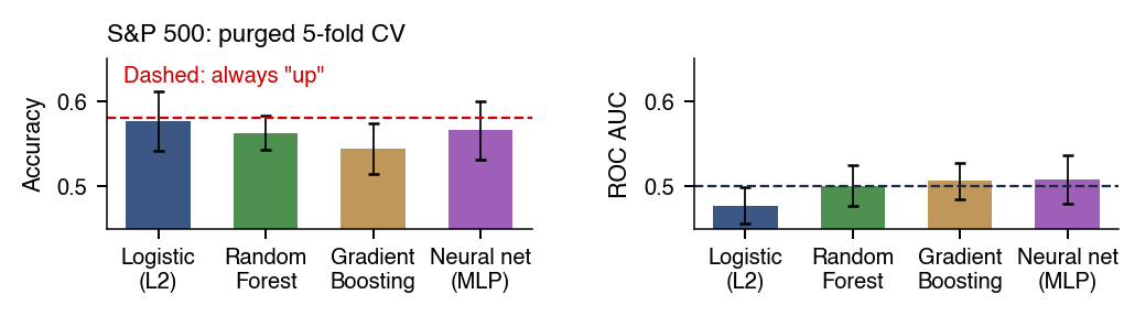
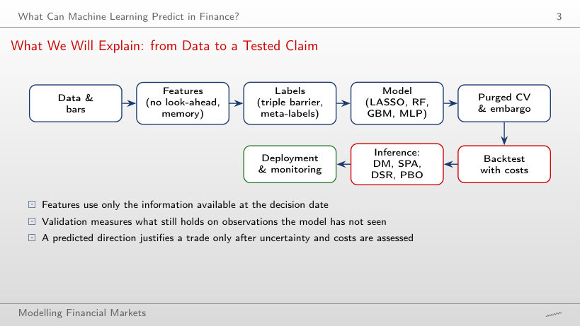
 MFM_ch13_model_comparison
 Random Forests