Bucharest University of Economic Studies IDA Institute Digital Assets Blockchain Research Center AI4EFin Artificial Intelligence for Energy Finance Romanian Academy, Institute for Economic Forecasting MSCA Digital Finance
“We present and justify a set of four desirable properties for measures of risk, and call the measures satisfying these properties ‘coherent.’ ” — Artzner, Delbaen, Eber & Heath (1999)
S&P 500 (Standard & Poor's), 2000–2026: historical VaR 1% (Value-at-Risk, the loss exceeded on 1% of days) is 3.45%
ES 1% (Expected Shortfall, the mean loss on the worst 1% of days) is 5.03%; the largest loss is 12.77% (16 March 2020)
Two independent bonds, each losing 100 with probability 0.9%: VaR 1% is 0 for each bond and 100 for the pair
ES 1% is 90 for each bond and 100.81 for the pair, below the sum of 180
Over the last 500 days, ES 2.5% rests on only \(n\alpha = 12.5\) losses
its HAC (heteroskedasticity and autocorrelation consistent) interval is 2.55 percentage points wide
Days with a loss above the one-day VaR 1%, 2006–2026 (target 1%)
1.67% for 500-day historical simulation, 1.54% for filtered historical simulation (FHS), 2.34% for GARCH (Generalised AutoRegressive Conditional Heteroskedasticity) with Normal shocks
The chapter starts from the question of how large tomorrow's tail losses are and how precisely we can estimate them. Value-at-Risk (VaR) gives the loss threshold exceeded with a small probability, Expected Shortfall (ES) the mean loss beyond that threshold. On S&P 500 (Standard & Poor's) daily losses over 2000–2026, the historical VaR 1% is 3.45%: the loss exceeded it on 68 of 6,717 days. ES 1%, the average loss over the worst 1% of days, is 5.03%. The largest loss, 12.77% on 16 March 2020, is about ten standard deviations; the Normal distribution fits the centre but is far too thin in the tail.
Artzner, Delbaen, Eber & Heath (1999) stated four properties that a risk measure should have and called the measures satisfying them coherent. VaR violates one of them, subadditivity. Two independent bonds, each losing 100 with probability 0.9%, each have a VaR 1% of 0, while their portfolio has a VaR 1% of 100. A VaR limit would therefore reward concentration. ES 1% is 90 for each bond and 100.81 for the portfolio, below the sum of 180. Precision is the second problem: over the last 500 days, ES 2.5% rests on only 12.5 losses, and its HAC (heteroskedasticity and autocorrelation consistent) interval is 2.55 percentage points wide.
Tomorrow's risk is a conditional question. Over 2006–2026, the share of days with a loss above the one-day VaR 1%, against a target of 1%, is 1.67% for 500-day historical simulation, 1.54% for filtered historical simulation (FHS) and 2.34% for GARCH (generalised autoregressive conditional heteroskedasticity) with Normal shocks. The historical window reacts months late, and its exceedances cluster in 2008 and 2020; the filtered VaR peaked at 18.01% on 18 March 2020. Even FHS has 80 exceedances in 5,210 days against 52.1 expected, and the Kupiec test rejects its coverage. The chapter goes on to extreme value theory, the 10-day horizon, the risk contributions of a portfolio and the Basel rules.
Conditional VaR and ESFiltered historical simulation and direct quantile models (CAViaR).
Extreme Value TheoryBlock maxima and the GEV (Generalised Extreme Value, distribution) distribution, peaks over threshold and the GPD, conditional EVT (Extreme Value Theory).
The chapter measures the risk of a position by the size of its rare large losses. Two numbers do this throughout: Value-at-Risk (VaR), a loss threshold exceeded with a small probability, and Expected Shortfall (ES), the mean loss beyond that threshold. Before either can be defined, four conventions must be fixed: which series are studied and in which units, how a loss is signed, over how many days it is measured, and how small the tail probability is.
How Large Are Daily Tail Losses, and How Precisely Can We Estimate Them?
The running example is the S&P 500, with daily data from 2000 to 2026. The results are compared with four other series: BET, the main index of the Bucharest Stock Exchange (BVB), Bitcoin, the EUR (euro)/RON exchange rate and gold. For EUR/RON the series is the reference rate of the National Bank of Romania (BNR). All data end on 18 September 2026; the full inventory, with the number of days in each series, is in the Appendix.
Returns are daily log returns in percent, \(r_t = 100\,(\ln P_t - \ln P_{t-1})\), where \(P_t\) is the closing price on day \(t\). The sample starts in 2000 so that it spans three crises: 2000–2002, 2008 and 2020. A tail measure at the 1% level rests on the worst one per cent of days, and only a sample that contains several crises holds enough extreme losses to estimate it.
In brief
Running example: S&P 500 daily losses, 2000–2026
comparisons on BET (main index of the Bucharest Stock Exchange, BVB), Bitcoin, EUR (euro)/RON and gold
EUR/RON: the reference rate of the National Bank of Romania (BNR), in Romanian lei (RON) per euro (EUR)
data up to 18 September 2026 (full inventory in the Appendix)
Units: daily log returns in %, \(r_t = 100\,(\ln P_t - \ln P_{t-1})\), with \(P_t\) the closing price on day \(t\)
Why 2000–2026: the sample spans three crises (2000–2002, 2008, 2020)
A bank's management and its supervisors need a single number that summarises the market risk of a trading book: a loss that is exceeded only rarely. The number serves two purposes, setting trading limits for desks and setting the capital that must absorb losses.
The return of the position over one day is \(X_{t+1} = r_{t+1}\), the log return in percent, and the loss is its negative, \(L_{t+1} = -X_{t+1}\). A positive \(L\) means that the position lost money. Because \(r\) is a log return, \(L\) is a log loss. If \(V_t\) is the value of the position, the loss in money is \(V_t\,(1 - e^{-L_{t+1}/100})\), which is close to \(V_t L_{t+1}/100\) when \(L\) is small.
Log returns are used because they add up over days, which is what the horizon \(h\) requires; simple returns add up across assets, which is what the portfolio requires, and the portfolio section switches to them. The map \(L \mapsto 1 - e^{-L/100}\) is increasing, so a quantile of the log loss converts directly into a quantile of the money loss: VaR in money is \(V_t(1 - e^{-\mathrm{VaR}_\alpha/100})\). ES is a mean, not a quantile, and the conversion does not pass through it; ES in money is computed scenario by scenario and then averaged.
The sign convention of the chapter is that VaR and ES are positive numbers when they represent losses.
In brief
Return over one day: \(X_{t+1} = r_{t+1}\), the log return in %
Loss: \(L_{t+1} = -X_{t+1}\), a log loss
\(L > 0\) means the position lost money
In money, with \(V_t\) the value of the position: loss \(= V_t\,(1 - e^{-L_{t+1}/100}) \approx V_t L_{t+1}/100\) for small \(L\)
Why log: log returns add over days, simple returns add across assets
over days: the horizon \(h\); across assets: the portfolio
The map \(L \mapsto 1 - e^{-L/100}\) is increasing
so VaR in money is \(V_t(1 - e^{-\VaR_\alpha/100})\)
ES in money is computed scenario by scenario, then averaged
Sign convention: VaR and ES are positive numbers when they are losses
Horizon and Level: Why 1 Day, 10 Days, 1% and 2.5%
Two choices define every risk number in the chapter. The horizon\(h\) is the number of days over which the loss is measured. One day is the horizon of trading limits and of backtesting, because a new observation arrives every day. Ten days is the time that the Basel rules assume is needed to liquidate a position (Basel Committee, 1996).
The level\(\alpha\) is the tail probability, and the chapter writes "VaR 1%" and "ES 2.5%". The level \(\alpha = 1\%\) is the VaR level of the 1996 amendment to the Basel Accord (Basel Committee, 1996): one exceedance every 100 days on average. The level \(\alpha = 2.5\%\) is the ES level of the Fundamental Review of the Trading Book (FRTB) (Basel Committee, 2019). It was chosen because, under the Normal distribution, ES 2.5% is close to VaR 1%, so the switch of measure does not by itself change capital for thin-tailed positions.
In brief
Horizon\(h\): the number of days over which the loss is measured
\(h = 1\) day: the horizon of trading limits and of backtesting (comparing forecasts with realised losses), with a new observation every day
\(h = 10\) days: the time Basel assumes for liquidating a position Basel Committee (1996)
Level\(\alpha\): the tail probability
we write “VaR 1%”, “ES 2.5%”
\(\alpha = 1\%\): the VaR level of the 1996 Basel amendment Basel Committee (1996), one exceedance every 100 days on average
chosen because under the Normal distribution ES 2.5% is close to VaR 1%
Section summary
Losses are positive, measured in log percent, over one or ten days, at the levels 1% and 2.5%. The next section defines VaR and ES precisely and computes them for the S&P 500.
Value-at-Risk and Expected Shortfall
This section answers two questions:
Which loss is exceeded on only a fraction \(\alpha\) of days? VaR, a quantile, answers it.
How much is lost, on average, beyond it? ES, a tail mean, answers it.
Both are computed for the S&P 500, and closed forms are derived for the Normal and the Student-\(t\) distributions.
For small \(\alpha\) the quantile \(q_\alpha(X)\) is negative, so the sign change in (7.1) makes VaR a positive loss. For a continuous loss \(L = -X\), the same number is the upper quantile of the loss, \(\mathrm{VaR}_\alpha = q_{1-\alpha}(L)\), and it is exceeded with probability exactly \(\alpha\). For a general distribution, with atoms, the probability of exceeding VaR is at most \(\alpha\).
VaR 1% reads: with probability 1%, tomorrow's loss will exceed \(\mathrm{VaR}_{1\%}\). The definition says nothing about how large the loss is when the threshold is crossed. Two positions with the same VaR can have very different losses on the worst days, and this is the gap that ES fills.
In brief
The question of this section: which loss is exceeded on only a fraction \(\alpha\) of days?
and how much do we lose, on average, beyond it?
VaR at level \(\alpha\): the loss exceeded with probability \(\alpha\) (exactly for continuous \(L\), at most \(\alpha\) in general)
where \(u\) is the integration variable, a tail probability between 0 and \(\alpha\). Because every \(\mathrm{VaR}_u\) with \(u < \alpha\) is at least \(\mathrm{VaR}_\alpha\), the average satisfies \(\mathrm{ES}_\alpha \ge \mathrm{VaR}_\alpha\): VaR looks at the entrance of the tail, ES into it.
For a continuous distribution, (7.2) is the mean loss on the days beyond VaR, \(\mathrm{ES}_\alpha(X) = -\mathbb{E}[X \mid X \le q_\alpha(X)]\). The quantile form (7.2) is preferred because it remains correct when the distribution has atoms, as in the two-bond example of the next section, where the conditional mean would give the wrong answer. The same measure appears as Conditional VaR (CVaR), Tail VaR and Average VaR in Rockafellar & Uryasev (2002) and Acerbi & Tasche (2002).
In brief
Expected Shortfall: the average of all quantiles in the tail of probability \(\alpha\)
Question for the room Increase each of the ten largest S&P 500 losses by 1 pp, leaving all other observations unchanged. What happens to historical VaR 1% and ES 1%?
Answer
VaR stays at 3.45%, and ES rises from 5.03% to about 5.18%. The ten modified losses lie above the observations that determine the quantile, so VaR does not change. ES 1% averages the largest nα = 67.17 losses (the last one with weight 0.17); all ten enter with weight 1, so ES rises by 10/67.17 ≈ 0.15 pp. VaR locates the threshold; ES also accounts for the severity of the losses beyond it. The Normal distribution with the same mean and standard deviation gives a VaR 1% of 2.80% and an ES 1% of 3.21%.
The chart compares the daily losses of the S&P 500 over 2000–2026 with the Normal distribution that has the same mean and standard deviation. The left panel shows the whole distribution, the right panel only the tail of large losses, where the historical VaR and ES are marked. The slider sets the level \(\alpha\) and ▶ moves it step by step; the readout gives, for each level, the historical VaR, the number of days on which it was exceeded and the historical ES, next to the Normal values.
The historical VaR 1% of the S&P 500 is 3.45%: on 68 of 6,717 days, 1.01% of the sample, the loss was larger. The historical ES 1%, the average loss over the worst 1% of days, is 5.03%. At the 2.5% level the historical VaR is 2.51% and the ES is 3.76%. The largest loss in the sample, 12.77% on 16 March 2020 during the COVID-19 crash, is about ten standard deviations.
The Normal distribution with the same mean and standard deviation fits the centre of the distribution but is far too thin in the tail, the stylised fact documented in Chapter 1. The numbers are a description of the sample: they say how large the worst losses were, not how large tomorrow's will be.
In brief
Daily losses 2000–2026 against the Normal distribution with the same mean and standard deviation
left: the whole distribution; right: the tail
Historical \(\VaR_{1\%} = 3.45\%\): 68 of 6 717 days (\(1.01\%\)) lost more
\(\ES_{1\%} = 5.03\%\) is the average loss over the worst 1% of days
At the 2.5% level: historical VaR is \(2.51\%\) and ES is \(3.76\%\)
largest loss \(12.77\%\) on 2020-03-16 (COVID-19 crash), about ten standard deviations
The Normal distribution fits the centre but is far too thin in the tail (Chapter 1)
Type of evidence: description (it shows what happened in the data, without testing a cause)
The Normal case gives closed forms that serve as a benchmark. Let \(X \sim N(\mu, \sigma^2)\), and let \(\Phi\) and \(\varphi\) be the distribution function and the density of the standard Normal distribution. The standard Normal quantile is \(z_\alpha = \Phi^{-1}(\alpha) < 0\), for example \(z_{1\%} = -2.326\). Since \(q_\alpha(X) = \mu + \sigma z_\alpha\), VaR is the mean minus \(|z_\alpha|\) standard deviations, with the sign changed.
For ES, substituting \(X = \mu + \sigma Z\) into the tail mean gives \(\mathrm{ES}_\alpha = -\mu - \frac{\sigma}{\alpha}\int_{-\infty}^{z_\alpha} u\varphi(u)\,du\); since \(\varphi'(u) = -u\varphi(u)\), the integral equals \(-\varphi(z_\alpha)\). Hence
Both measures in (7.3) have the same form: minus the mean plus a multiple of \(\sigma\). ES replaces the factor \(-z_\alpha\) by the larger factor \(\varphi(z_\alpha)/\alpha\), the Mills-ratio form of the Normal tail mean.
In brief
Setting: \(X \sim N(\mu, \sigma^2)\), a Normal return with mean \(\mu\) and standard deviation \(\sigma\)
\(\Phi\), \(\varphi\): the distribution function and the density of the standard Normal distribution \(N(0, 1)\)
\(z_\alpha = \Phi^{-1}(\alpha) < 0\): the standard Normal \(\alpha\)-quantile, e.g. \(z_{1\%} = -2.326\)
VaR: the mean minus \(|z_\alpha|\) standard deviations, sign changed
\(\VaR_\alpha = -(\mu + \sigma z_\alpha)\)
ES: the same form, with the larger factor \(\varphi(z_\alpha)/\alpha\) in place of \(-z_\alpha\)
The constants of (7.3) are worth remembering. At 1%, \(-z_{1\%} = 2.326\) and \(\varphi(z_{1\%})/0.01 = 2.665\); at 2.5%, \(-z_{2.5\%} = 1.960\) and \(\varphi(z_{2.5\%})/0.025 = 2.338\). Under the Normal distribution, ES 2.5% is therefore almost equal to VaR 1%, 2.338 against 2.326 standard deviations, which is the calibration behind the FRTB level.
For the S&P 500, with \(\hat\mu = 0.025\%\) and \(\hat\sigma = 1.213\%\), the Normal VaR 1% is \(-0.025 + 1.213 \times 2.326 \approx 2.80\%\), against the historical 3.45%; the historical VaR is 1.24 times the Normal one. Under the Normal distribution and for a given mean, VaR and ES carry no information beyond \(\sigma\): they are fixed multiples of it. Any tail behaviour that the data show beyond the standard deviation must therefore come from a different model.
The simplest heavy-tailed alternative shifts and rescales a Student-\(t\) variable: \(X = m + s\,T\) with \(T \sim t_\nu\). Here \(m\) is the location, \(s > 0\) the scale and \(\nu\) the degrees of freedom; a smaller \(\nu\) means heavier tails. Let \(t_\alpha = t_\nu^{-1}(\alpha) < 0\) be the \(\alpha\)-quantile and \(g_\nu\) the density of \(t_\nu\). VaR has the same form as for the Normal distribution, while ES acquires an extra factor:
The factor \((\nu + t_\alpha^2)/(\nu - 1)\) in (7.4) exceeds 1 and accounts for the heavy tail; ES exists only for \(\nu > 1\), because the tail mean is infinite otherwise. The variance of \(X\) is \(s^2\nu/(\nu - 2)\) and exists only for \(\nu > 2\), so the scale \(s\) is not the standard deviation. A fit to the S&P 500, step by step, is in Further Topics.
In brief
Model: the return is a shifted and rescaled Student-\(t\) variable, \(X = m + s\,T\) with \(T \sim t_\nu\)
VaR is a quantile and ES the average of the quantiles beyond it. On the S&P 500, VaR 1% is 3.45% and ES 1% is 5.03%, both well above the Normal values. The Normal and Student-\(t\) formulas (7.3) and (7.4) express both measures as location plus a multiple of scale. The next section asks which of the two measures should be used as capital.
Coherent Risk Measures
A risk measure used for capital must behave sensibly when positions are scaled, shifted or combined. Artzner, Delbaen, Eber & Heath (1999) stated four axioms for this, and this section shows that ES satisfies all of them while VaR can violate subadditivity. Two further properties complete the comparison: robustness, which favours VaR, and elicitability, which determines how forecasts of each measure can be evaluated.
A risk measure\(\rho\) maps a loss \(L\), a random variable, to the amount of capital to hold against it. Let \(L_1, L_2\) be two losses, \(c\) a sure amount and \(\lambda \ge 0\) a scaling factor. The measure is coherent (Artzner, Delbaen, Eber & Heath, 1999) if it is monotone, \(L_1 \le L_2 \Rightarrow \rho(L_1) \le \rho(L_2)\); translation invariant, \(\rho(L + c) = \rho(L) + c\); positively homogeneous, \(\rho(\lambda L) = \lambda\rho(L)\); and subadditive,
\[\rho(L_1 + L_2) \le \rho(L_1) + \rho(L_2).\]
(7.5)
Each axiom has a direct reading. A position that always loses more needs more capital. Adding a sure loss \(c\) raises the capital by exactly \(c\). Doubling the position doubles the capital. And by (7.5), merging two positions never needs more capital than holding them apart: diversification does not add risk.
In brief
The question: which properties must a number used as capital have?
so that diversification is never penalised
A risk measure\(\rho\) maps a loss \(L\) (a random variable) to the capital to hold
Subadditivity has two consequences in practice. For limits, it guarantees that the risk of the whole bank does not exceed the sum of the risk limits of its desks, \(\sum_i \rho_i\), and it rules out regulatory arbitrage by splitting a firm into separately capitalised units. For optimisation, positive homogeneity and subadditivity together make \(\rho\) convex in the portfolio weights, so every local minimum of risk is a global one. Uniqueness of the minimum would need strict convexity, which ES computed from scenarios does not have, since it is piecewise linear in the weights.
VaR satisfies the first three axioms but not, in general, subadditivity. The exception is the class of jointly elliptical losses, such as the multivariate Normal or Student-\(t\), at levels \(\alpha < 50\%\). There VaR and ES are both of the form \(\mu_p + \sigma_p \times\) constant, where \(\mu_p\) and \(\sigma_p\) are the mean and standard deviation of the portfolio loss (McNeil, Frey & Embrechts, 2015), and subadditivity follows from that of \(\sigma_p\). Refinements for heavy tails are in the Appendix.
In brief
Limits
By subadditivity, bank-wide risk does not exceed the sum of the desk risk limits, \(\sum_i \rho_i\)
No regulatory arbitrage by splitting a firm
Optimisation: homogeneity + subadditivity \(\Rightarrow\) convexity in the portfolio weights
Every local minimum is global; uniqueness would need strict convexity, which scenario-based ES lacks (it is piecewise linear)
VaR satisfies the first three axioms, but not subadditivity in general
Exception: jointly elliptical losses (multivariate Normal or Student-\(t\)) and \(\alpha < 50\%\), where VaR and ES are both \(\mu_p + \sigma_p\times\) constant McNeil, Frey & Embrechts (2015)
\(\mu_p\), \(\sigma_p\): mean and standard deviation of the portfolio loss (heavy-tailed refinements: Appendix)
The standard counterexample uses two independent bonds, A and B. Each loses 100 if it defaults, with probability \(p = 0.9\%\), and 0 otherwise. Because the loss is discrete, ES must be computed from the quantile form (7.2), which for a discrete loss \(L\) gives
The first term of (7.6) collects the losses strictly beyond VaR; the second places the rest of the tail probability \(\alpha\) at VaR itself. Here \(\mathbf{1}\{\cdot\}\) is the indicator function.
For one bond, the probability of losing 100 is 0.9%, not above 1%, so the 1% quantile of the value change is 0 and \(\mathrm{VaR}_{1\%}(A) = \mathrm{VaR}_{1\%}(B) = 0\). By (7.6),\(\mathrm{ES}_{1\%}(A) = (100 \times 0.009 + 0 \times 0.001)/0.01 = 90\). For the portfolio, the probability of losing at least 100 is \(1 - (1-p)^2 = 1.79\% > 1\%\), while the probability of losing 200 is only \(p^2 = 0.0081\%\); the 1% quantile is therefore \(-100\) and \(\mathrm{VaR}_{1\%}(A + B) = 100\), more than the sum \(0 + 0\) of the stand-alone values. ES behaves as the axiom requires: \(\mathrm{ES}_{1\%}(A + B) = 100.81\), below \(\mathrm{ES}_{1\%}(A) + \mathrm{ES}_{1\%}(B) = 180\).
In brief
Bonds A and B, independent: each loses 100 with probability \(p = 0.9\%\) (default)
and 0 otherwise
\(X\): the value change, \(X = -L\)
General formula for a discrete loss \(L = -X\): \(\ES_\alpha = \frac{1}{\alpha}\left(\E[L\,\mathbf{1}\{L > \VaR_\alpha\}] + \VaR_\alpha\,(\alpha - P(L > \VaR_\alpha))\right)\)
\(\mathbf{1}\{\cdot\}\): indicator, 1 if the condition holds and 0 otherwise; first term: losses strictly beyond VaR; second term: the rest of the tail probability \(\alpha\), placed at VaR itself
One bond: \(P(X \le -100) = p = 0.9\%\), not above \(1\%\), so \(q_{1\%} = 0\) and \(\VaR_{1\%}(A) = \VaR_{1\%}(B) = 0\)
The chart puts the two measures side by side for the bonds of the previous frame: in blue the sum of the two stand-alone measures, in red the measure of the combined portfolio. The slider changes the default probability of each bond, and ▶ runs it from 0.1% to 2%.
Question for the room Keep the two bonds independent, with a loss of 100 on each default. If each bond’s default probability rises from 0.9% to 1.1%, what is the portfolio VaR 1%?
Answer
100. The probability that at least one defaults becomes 2.19%, above 1%, but the probability of two defaults is only 0.012%, below 1%; the portfolio VaR 1% stays at 100. Each individual VaR becomes 100, so their sum is 200 ≥ 100 and subadditivity holds: 200 is the sum of the individual VaRs, not the portfolio VaR, and 0 was the individual VaR at 0.9%. At 0.9% (the slide), the probability of at least one default is 1.79%, and the portfolio VaR, 100, exceeds the sum 0 + 0. In this example, VaR violates subadditivity only when the default probability lies between about 0.5% and 1%. ES is subadditive: at 0.9%, 100.8 for the portfolio against 90 + 90 = 180.
At the default probability of 0.9%, the red VaR bar, 100, exceeds the blue one, \(0 + 0\), which is the violation of (7.5); for ES the red bar, 100.81, lies below the blue one, 180.
The consequence for risk management is that a limit expressed in VaR would reward concentration: holding only bond A looks riskless, holding both does not. ES sees the size of the tail and is coherent (Acerbi & Tasche, 2002). In practice VaR fails in this way for credit portfolios, options and other skewed pay-offs, where the loss distribution has a small probability of a large loss.
In brief
Blue: sum of the two stand-alone measures
red: the measure of the combined portfolio
VaR jumps from \(0 + 0\) to 100 when the bonds are combined (the counterexample of the previous slide)
A VaR limit would reward concentration: holding only A looks riskless
The quick check compares two positions with losses in percent at the level \(\alpha = 10\%\). Position A has a loss uniform on \([0, 10]\); position B loses 0 with probability 0.95 and 20 with probability 0.05. VaR and ES follow from the definitions (7.1) and (7.2), for B with the discrete formula (7.6). The point of the exercise is to see which position each measure calls riskier and what VaR does not see. The answers are in the Appendix.
In brief
Two positions, losses in %, level \(\alpha = 10\%\)
A: loss \(L_A\) uniform on \([0, 10]\), every value equally likely
Find \(\VaR_{10\%}(A)\) and \(\ES_{10\%}(A)\) from the definitions
B: loss 0 with probability \(0.95\), loss 20 with probability \(0.05\)
Find \(\VaR_{10\%}(B)\) and \(\ES_{10\%}(B)\) with the discrete ES formula of the two-bond slide
Coherence is not the only desirable property of a risk measure; an estimate should also be stable. Qualitative robustness (Cont, Deguest & Scandolo, 2010) requires that a small change in the distribution of the data changes the law of the estimator only a little. Historical VaR is qualitatively robust at distributions with a unique \(\alpha\)-quantile. Historical ES is not: a single extreme loss can move it without bound, as the precision section shows.
The effect is visible on the last 500 days of the S&P 500. Dropping the single largest loss, 6.16% on 4 April 2025, moves ES 2.5% from 2.98% to 2.64%, but VaR 1% only from 2.73% to 2.68%. The trade-off is structural: subadditivity requires the measure to look beyond the quantile, and this is exactly what makes it sensitive to single observations. FRTB resolved it by using ES 2.5% for capital and keeping VaR for backtesting, because VaR is robust and VaR forecasts can be compared directly through a score.
a small change in the data distribution changes the law of the estimator only a little
Historical VaR is qualitatively robust at distributions with a unique \(\alpha\)-quantile; historical ES is not: one extreme loss moves it without bound (the precision section)
S&P 500, last 500 days: drop the single largest loss (\(6.16\%\), 2025-04-04)
A forecast is evaluated with a scoring function\(S(v, X)\), a penalty computed from the forecast \(v\) and the outcome \(X\); lower means better. A risk measure is elicitable if it is the unique minimiser of \(\mathbb{E}[S(v, X)]\) for some \(S\), which is then called strictly consistent. VaR is elicitable: the quantile \(q_\alpha(X)\) minimises the expected pinball loss
which charges \(1 - \alpha\) per unit when \(X\) falls below \(v\) and \(\alpha\) per unit when it stays above. Strict consistency means that a forecaster who reports anything other than the true quantile has a higher expected score.
ES alone is not elicitable (Gneiting, 2011): no strictly consistent scoring function exists for ES on its own. The pair (VaR, ES), however, is jointly elicitable (Fissler & Ziegel, 2016). Joint scores such as FZ0, the Fissler–Ziegel score in the form of Patton, Ziegel & Chen (2019), rank (VaR, ES) forecasts. For FZ0, \(S(cv, ce; cY) = S(v, e; Y) + \ln c\), so score differences, not the score itself, are homogeneous of degree zero. The scores are used to estimate models in the Appendix and to evaluate forecasts in Chapter 8.
In brief
A scoring function\(S(v, X)\): a penalty computed from the forecast \(v\) and the outcome \(X\)
lower means a better forecast
A risk measure is elicitable if it is the unique minimiser of \(\E[S(v, X)]\) for some \(S\)
such an \(S\) is a strictly consistent score
VaR: the quantile \(q_\alpha(X)\) minimises the pinball loss \(\E[(\mathbf{1}\{X \le v\} - \alpha)(v - X)]\)
The pinball loss charges \(1 - \alpha\) per unit when \(X\) falls below \(v\) and \(\alpha\) per unit when it stays above
\(S(cv, ce; cY) = S(v, e; Y) + \ln c\): score differences, not the score itself, are homogeneous of degree zero
Section summary
ES satisfies the four axioms of coherence, VaR fails subadditivity, and the two-bond example shows that a VaR limit can reward concentration. In exchange, historical ES is not robust to a single extreme loss, and ES alone is not elicitable, while (VaR, ES) is. FRTB uses ES for capital and VaR for backtesting.
Estimation Methods
This section turns the definitions into estimators. The question is how VaR and ES are estimated from data, and how much the answer depends on the assumption made about the tail. Historical simulation makes no assumption; the Normal, Student-\(t\) and Cornish–Fisher methods impose a parametric shape; the extreme value method, previewed here, fits only the tail.
Historical simulation takes the last \(n\) daily losses \(L_{t-n+1}, \dots, L_t\) and sorts them, \(L_{(1)} \le \dots \le L_{(n)}\), where \(L_{(i)}\) is the \(i\)-th smallest loss. VaR is the empirical \((1-\alpha)\)-quantile, interpolated linearly, and ES integrates the empirical quantile function over the worst fraction \(\alpha\) of the losses:
with \(\ell = 1 + (n-1)(1-\alpha)\),\(j = \lfloor \ell \rfloor\) and \(m = \lfloor n\alpha \rfloor\). In the ES estimator of (7.8) the \(m\) largest losses get weight 1 and the next one, \(L_{(n-m)}\), gets the fractional weight \(n\alpha - m\). An alternative estimator averages the \(k_\alpha\) losses at or above \(\widehat{\mathrm{VaR}}_\alpha\); it differs from (7.8) when \(n\alpha\) is not an integer.
The window length \(n\) trades reaction speed against precision: 250 days react faster, 1,000 days give more precise estimates. With \(n = 500\), only 5 losses lie beyond VaR 1%, and ES 2.5% gives weight 1 to the 12 largest losses and weight 0.5 to the 13th, since \(n\alpha = 12.5\).
The method has two structural limits:
No loss larger than the worst one in the window can appear in the estimate.
A crash day enters the window, stays there for \(n\) days and then drops out, so VaR falls abruptly on a day when nothing happened: the ghost effect.
In brief
The question of this section: how do we estimate VaR and ES from data?
and how much does the answer depend on the tail assumption?
Take the last \(n\) daily losses \(L_{t-n+1}, \dots, L_t\) and sort them: \(L_{(1)} \le \dots \le L_{(n)}\)
\(L_{(i)}\): the \(i\)-th smallest loss
\(\widehat{\VaR}_\alpha = L_{(j)} + (\ell - j)\,(L_{(j+1)} - L_{(j)})\), with \(\ell = 1 + (n-1)(1-\alpha)\) and \(j = \lfloor \ell \rfloor\): the empirical \((1-\alpha)\)-quantile, interpolated linearly
\(\widehat{\ES}_\alpha = \frac{1}{n\alpha}\big[\sum_{i=1}^{m} L_{(n-i+1)} + (n\alpha - m)\,L_{(n-m)}\big]\), with \(m = \lfloor n\alpha \rfloor\): the integral of the empirical quantile function over the worst fraction \(\alpha\) of the losses
The \(m\) largest losses get weight 1; the next one, \(L_{(n-m)}\), gets the fractional weight \(n\alpha - m\)
Alternative, the mean of the selected exceedances: the simple mean of the \(k_\alpha\) losses \(\ge \widehat{\VaR}_\alpha\); it differs from \(\widehat{\ES}_\alpha\) when \(n\alpha\) is not an integer
Choice of window \(n\): 250 days reacts faster, 1000 days is more precise
With \(n = 500\): 5 losses lie beyond VaR 1%; ES 2.5% gives weight 1 to the 12 largest losses and weight 0.5 to the 13th (\(n\alpha = 12.5\))
No loss beyond the worst one in the window can appear in the estimate
Ghost effect: a crash day enters the window, stays for \(n\) days, then drops out and VaR falls abruptly
Cornish–Fisher: Correcting the Normal Quantile, and Where It Breaks
The Cornish–Fisher expansion (Cornish & Fisher, 1938) corrects the Normal quantile for the skewness \(S = \mathbb{E}[(X - \mu)^3]/\sigma^3\) and the excess kurtosis \(K = \mathbb{E}[(X - \mu)^4]/\sigma^4 - 3\) of the returns:
With \(S = K = 0\),(7.9) gives back the Normal VaR. For \(\alpha\) below about 4%, where \(|z_\alpha| > \sqrt{3}\), negative skewness (a long left tail of returns) and positive excess kurtosis (heavy tails) push \(\tilde z_\alpha\) further below \(z_\alpha\) and raise VaR, while the \(S^2\) term pushes the other way; at \(\alpha = 5\%\) the kurtosis term has the opposite sign. ES is obtained numerically, by averaging \(-(\mu + \sigma\tilde z_u)\) over \(u \in (0, \alpha)\).
The expansion is built around the Normal distribution and is accurate only for small \(S\) and \(K\); for large \(K\) the map \(z \mapsto \tilde z\) is not even monotone. The S&P 500 has \(S = -0.35\) and \(K = 10.7\), far outside that range, and the sample kurtosis itself presupposes a finite fourth moment, which Chapter 1 questions. The result is a Cornish–Fisher VaR 1% of 6.08% against the historical 3.45%: the kurtosis term overshoots.
In brief
Adjust the Normal quantile for skewness\(S = \E[(X - \mu)^3]/\sigma^3\) and excess kurtosis\(K = \E[(X - \mu)^4]/\sigma^4 - 3\)Cornish & Fisher (1938)
\(\tilde z_\alpha\): the corrected quantile; \(S = K = 0\) gives back the Normal VaR
For \(\alpha\) below about \(4\%\) (\(|z_\alpha| > \sqrt{3}\)): \(S < 0\) (long left tail of returns) or \(K > 0\) (heavy tails) push \(\tilde z_\alpha\) further below \(z_\alpha\) and raise VaR; the \(S^2\) term pushes the other way. At \(\alpha = 5\%\) the \(K\) term has the opposite sign
ES: average of \(-(\mu + \sigma\tilde z_u)\) over \(u \in (0, \alpha)\), numerically
An expansion around the Normal distribution: accurate only for small\(S\) and \(K\)
for large \(K\) the map \(z \mapsto \tilde z\) is not even monotone (Seminar 7, A6)
S&P 500 returns: \(S = -0.35\), \(K = 10.7\): far outside that range
the sample \(K\) requires a finite fourth moment, which Chapter 1 questions
\(\VaR_{1\%}^{CF} = 6.08\%\) versus historical \(3.45\%\): the kurtosis term overshoots
Question for the room Where is the gap between the largest and the smallest VaR estimated by the five methods greater: at α = 5% or at α = 0.1%?
Answer
At α = 0.1%: the gap is 11.34 pp (Cornish–Fisher 15.06% minus the Normal distribution 3.72%), against 0.30 pp at α = 5%, where all five values lie between 1.67% and 1.97%. At α = 0.1%, VaR is 7.22% historical, 7.04% with EVT and 8.58% with Student-t. Where data are scarce, the tail assumptions drive the estimate: the same statistical target does not force different models to give close values.
The chart compares five methods over a range of tail probabilities for the S&P 500 daily losses of 2000–2026. The horizontal axis gives \(\alpha\) from 5% down to 0.1% on a log scale; the vertical axis gives VaR (left panel) and ES (right panel) in percent. The methods are historical simulation (HS), the Normal distribution, the Student-\(t\) distribution, Cornish–Fisher and extreme value theory (EVT), here a generalised Pareto distribution (GPD) fitted to the tail, which is developed in the extreme value section. The slider moves a cursor along the \(\alpha\) axis, and the readout lists the five VaR and ES values at that level.
At VaR 0.1%, a loss exceeded on one day in four years on average, the methods disagree sharply. Historical simulation gives 7.22%, EVT 7.04%, the Student-\(t\) 8.58% and Cornish–Fisher 15.06%. The Normal distribution gives 3.72%, about half of the historical value.
The gap between methods grows as \(\alpha\) falls, and more for ES than for VaR, because ES depends on the whole tail beyond the quantile. EVT and historical simulation agree down to 0.5%; below that EVT extrapolates a fitted tail, while historical simulation is limited by the few largest observations. The comparison is between procedures; a comparison on five assets is in Further Topics.
In brief
Horizontal axis: \(\alpha\) from 5% down to 0.1%, log scale
vertical axis: VaR (left) and ES (right), S&P 500 daily losses 2000–2026, in %
legend: HS = historical simulation
EVT (extreme value theory) = a GPD (generalised Pareto distribution) tail, a preview of the Extreme Value Theory section
Historical simulation is the reference, but it cannot see beyond the worst loss in its window. The Normal distribution understates the tail, Cornish–Fisher overstates it for kurtosis as large as that of daily returns, and the differences between methods grow as the level falls. The next section asks how precise any of these estimates is.
How Precise Are VaR and ES?
An estimated VaR or ES is a statistic, and a different sample of the same length would give a different number. This section derives usable standard errors for historical VaR and ES, shows how volatility clustering widens them, and reports the resulting intervals for the S&P 500.
For VaR, assume i.i.d. (independent and identically distributed) losses with a density \(f\) that is continuous and positive at \(\mathrm{VaR}_\alpha\). The standard error (SE) of the historical estimate is
The factor \(\sqrt{\alpha(1 - \alpha)/n}\) in (7.10) is the SE of the share of days beyond VaR; dividing by the density \(f(\mathrm{VaR}_\alpha)\) converts this error in probability into an error on the loss scale. In the tail the density is small, so the SE is large.
With \(\sigma = 1.2\%\) and \(n = 500\), the SE of VaR 1% is 0.20 percentage points (pp) under the Normal distribution and 0.43 pp under a Student-\(t\) with 4 degrees of freedom (\(t_4\)) scaled to the same \(\sigma\). The heavier tail has a lower density at its 1% quantile, and the SE more than doubles.
In brief
The question of this section: how much would the estimated VaR and ES change on another sample of the same length?
VaR: i.i.d. (independent and identically distributed) losses with density \(f\) continuous and positive at \(\VaR_\alpha\)
\(\mathrm{SE}(\widehat{\VaR}_\alpha) \approx \dfrac{1}{f(\VaR_\alpha)}\sqrt{\dfrac{\alpha(1 - \alpha)}{n}}\) (SE: standard error)
\(\sqrt{\alpha(1 - \alpha)/n}\): the SE of the share of days beyond VaR; dividing by the density \(f(\VaR_\alpha)\) turns it into an error on the loss scale
The tail density is small, so the SE is large
\(\sigma = 1.2\%\), \(n = 500\): SE of \(\VaR_{1\%}\) = \(0.20\) percentage points (pp) under the Normal distribution, \(0.43\) pp under a \(t_4\) (Student-\(t\), 4 degrees of freedom) with the same \(\sigma\)
For ES, the starting point is the influence function of the historical estimator (Chen, 2008),\(\mathrm{IF}(x) = \mathrm{VaR}_\alpha + (x - \mathrm{VaR}_\alpha)_+/\alpha - \mathrm{ES}_\alpha\), where \((y)_+ = \max(y, 0)\). It measures the effect of one extra observation \(x\) on the estimate, and it grows without bound in \(x\): one extreme loss can move ES arbitrarily far. If \(\mathbb{E}[L^2] < \infty\), the standard error is
Estimating VaR adds no first-order term to (7.11), a consequence of the Rockafellar–Uryasev representation in Further Topics. As Yamai & Yoshiba (2005) and Pele & Mazurencu-Marinescu-Pele (2026) show, for Pareto-type tails with tail index \(a > 2\) the relative error falls like \(1/\sqrt{n\alpha}\), so the number of tail observations, not the sample size, governs precision.
Under volatility clustering the observations are not independent. The variances in (7.10) and (7.11) are then replaced by long-run HAC variances (Newey & West, 1987) of the series \(\mathbf{1}\{L_t > \mathrm{VaR}_\alpha\}\) and \((L_t - \mathrm{VaR}_\alpha)_+\), or the intervals are computed by a block bootstrap. Both constructions are described in Further Topics and the derivations in the Appendix.
In brief
ESChen (2008): influence function \(\mathrm{IF}(x) = \VaR_\alpha + (x - \VaR_\alpha)_+/\alpha - \ES_\alpha\), unbounded in \(x\)
\(\mathrm{IF}(x)\): the effect of one extra observation \(x\) on the estimate; it grows without bound with \(x\), so one extreme loss can move ES arbitrarily far
The standard error
If \(\E[L^2] < \infty\): \(\mathrm{SE}(\widehat{\ES}_\alpha) \approx \dfrac{1}{\alpha}\sqrt{\dfrac{\Var((L - \VaR_\alpha)_+)}{n}}\) ; \(\Var\): the variance; estimating VaR adds no first-order term (Rockafellar–Uryasev)
Replace the variances by long-run HAC (heteroskedasticity and autocorrelation consistent) variances Newey & West (1987) of \(\mathbf{1}\{L_t > \VaR_\alpha\}\) and \((L_t - \VaR_\alpha)_+\)
Or use a block bootstrap, which resamples blocks of consecutive days (derivations: Appendix)
Question for the room Which observations enter the historical ES 2.5% estimated on the last 500 days?
Answer
The tail mass is 500 × 0.025 = 12.5 observations: sum the 12 largest losses and 0.5 of the 13th, then divide by 12.5. With 13 equal weights, the effective tail level becomes 13/500 = 2.6%. The 95% HAC interval of this ES is 2.55 pp wide and the block bootstrap interval 2.42 pp. On the 2000–2026 sample, volatility clustering widens the ES interval from 0.60 pp (i.i.d.) to 1.00 pp (HAC), and the bootstrap interval from 0.62 pp to 1.17 pp.
The chart shows 95% intervals for the S&P 500 VaR 1% and ES 2.5% as bars, with the estimates marked by black ticks. Each interval is computed with the i.i.d. and HAC formulas and with the i.i.d. and block bootstraps, on the full 2000–2026 sample and on a recent window. The slider sets the length \(n\) of that recent window (rows 2 and 4 of the chart) and ▶ runs through the window lengths, so that the effect of \(n\alpha\) on the width of the intervals can be followed.
On the full sample, volatility clustering widens the ES interval from 0.60 pp under the i.i.d. formula to 1.00 pp with HAC; the bootstrap behaves in the same way, 0.62 pp for i.i.d. resampling against 1.17 pp by blocks. On the last 500 days, ES 2.5% rests on only \(n\alpha = 12.5\) losses and its HAC interval is 2.55 pp wide. The complete table is in the Appendix.
These intervals concern the unconditional VaR and ES, the risk averaged over the sample. Tomorrow's risk is a conditional question, treated in the next section. The HAC interval for ES also has conditions: a finite second moment of the excess beyond VaR, \(\mathbb{E}[(L - v)_+^2] < \infty\), which requires a tail index above 2 (estimated in Chapter 1), plus stationarity and weak dependence. GARCH quasi-maximum-likelihood inference, used in the next section, has its own condition, a finite fourth moment of the standardised innovations \(z_t\).
In brief
95% intervals (bars), with estimates marked by black ticks
Full sample: clustering widens the ES interval from \(0.60\) (i.i.d.) to \(1.00\) (HAC)
the bootstrap does the same: \(0.62\) i.i.d. vs \(1.17\) by blocks
last 500 days: ES 2.5% rests on only \(n\alpha = 12.5\) losses, HAC interval width \(2.55\) pp
These intervals cover the unconditional VaR and ES
tomorrow's risk is a conditional question (next section)
The HAC interval for ES requires a finite second moment of the excess beyond VaR, \(\E[(L - v)_+^2] < \infty\) (tail index above 2, estimated in Chapter 1), plus stationarity and weak dependence
GARCH-QML (GARCH Quasi-Maximum Likelihood) inference has its own conditions: a finite fourth moment of the standardised innovations \(z_t\)
The quick check applies (7.10) to i.i.d. Normal daily losses with mean 0 and \(\sigma = 1\%\) at the level \(\alpha = 5\%\), where \(\mathrm{VaR}_{5\%} = 1.645\%\) and the density at VaR is \(f(\mathrm{VaR}_{5\%}) = \varphi(1.645)/\sigma = 0.1031\). It asks for the SE and the 95% half-width with 1,000 days, the number of days that halves the SE, and the number of losses that historical ES 1% averages with 1,000 days. The answers are in the Appendix.
In brief
i.i.d. Normal daily losses with mean 0 and \(\sigma = 1\%\); level \(\alpha = 5\%\)
so \(\VaR_{5\%} = 1.645\%\)
the density there is \(f(\VaR_{5\%}) = \varphi(1.645)/\sigma = 0.1031\)
(a) With \(n = 1\,000\) days, what is the SE of historical \(\VaR_{5\%}\) and the half-width of its 95% interval?
(b) How many days halve that SE?
(c) With \(n = 1\,000\), how many losses does historical \(\ES_{1\%}\) average, and why is that a warning?
The SE of historical VaR depends on the tail density, that of ES on the variance of the excess beyond VaR, and both grow under volatility clustering. On the last 500 days of the S&P 500, ES 2.5% rests on 12.5 losses and its HAC interval is 2.55 pp wide. Every VaR or ES should therefore be reported with its tail count and an interval.
Conditional VaR and ES
The previous sections estimated the unconditional distribution of losses: the risk averaged over years. A trading desk needs tomorrow's risk, which depends on today's volatility. This section adapts VaR and ES to the current state of the market in two ways:
Filtered historical simulation (FHS) combines a volatility model with the empirical distribution of the shocks.
CAViaR models the quantile itself as a dynamic process.
The idea of FHS (Barone-Adesi, Giannopoulos & Vosper, 1999; Hull & White, 1998) is to take the shape of the shocks from history and their scale from a volatility model. The volatility model is GARCH (generalised autoregressive conditional heteroskedasticity) of Chapter 5(Bollerslev, 1986), with an AR(1) (autoregressive of order 1) conditional mean:
In (7.12),\(\mu_t\) is the conditional mean, with constant \(c\) and coefficient \(\phi\), and \(\sigma_t\) is the conditional volatility. The shocks \(z_t\) are i.i.d. with mean 0 and variance 1, and their distribution is left unspecified: that is the part history will supply. The constant is \(\omega > 0\);\(\alpha_1 \ge 0\) measures the reaction to yesterday's squared surprise and \(\beta_1 \ge 0\) the weight on yesterday's variance. Their sum \(\alpha_1 + \beta_1\) is the persistence, and \(\alpha_1 + \beta_1 < 1\) ensures a finite unconditional variance; a value close to 1 means that volatility shocks fade slowly. The coefficient \(\alpha_1\) should not be confused with the tail level \(\alpha\).
In brief
The question of this section: how do we adapt VaR and ES to today's volatility?
The AR(1)-GARCH(1,1) model is estimated by quasi-maximum likelihood (QML): the likelihood is Normal, but the estimates remain consistent when the shocks have another distribution.
The standardised residuals \(\hat z_t = (r_t - \hat\mu_t)/\hat\sigma_t\) are computed; they are approximately i.i.d. but still heavy-tailed.
The empirical tail of the residuals is rescaled by tomorrow's volatility forecast:
Here \(\hat\mu_{t+1}\) and \(\hat\sigma_{t+1}\) are the model forecasts for tomorrow, \(\hat\xi_\alpha\) is minus the empirical \(\alpha\)-quantile of the residuals, and \(\bar z_\alpha\) is the average of the lowest fraction \(\alpha\) of the residuals, with the fractional weight of historical simulation (7.8). The method replaces the Normal quantile \(z_\alpha\) of a GARCH-Normal model by an empirical one, so (7.13) keeps the volatility dynamics of GARCH without imposing a shock distribution. A worked forecast for the next trading day is in Further Topics.
In brief
Step 1: estimate the AR(1)-GARCH(1,1) model by quasi-maximum likelihood
Normal likelihood, robust to other shock distributions
Step 2: standardised residuals \(\hat z_t = (r_t - \hat\mu_t)/\hat\sigma_t\): approximately i.i.d., still heavy-tailed
\(\hat\mu_{t+1}\), \(\hat\sigma_{t+1}\): the model forecasts for tomorrow; \(\hat\xi_\alpha\): minus the empirical \(\alpha\)-quantile of the residuals (not the EVT shape \(\xi\))
\(\bar z_\alpha\): the average of the lowest fraction \(\alpha\) of the residuals \(\hat z_t\), with the fractional weight of historical simulation
Historical vs Filtered Historical Simulation: S&P 500 (1/2)
Question for the room In 2006–2026, which method comes closest to the 1% target for exceedances of VaR 1%?
Answer
FHS comes closest to the 1% target: 80 of 5,210 days, that is 1.54%, against 1.67% for historical simulation on 500 days and 2.34% for GARCH with Normal shocks. The historical window updates daily, but gives equal weight to observations from different volatility regimes and may adapt slowly; its exceedances come in clusters, in 2008 and 2020. Closeness to a 1% exceedance rate does not by itself establish independence of the exceedances.
The chart compares the two methods on the S&P 500 over 2006–2026. Bars show the daily loss; the lines are the one-day-ahead VaR forecasts, dark blue for 500-day historical simulation and red for FHS. Blue dots mark losses above the historical VaR and red crosses losses above the FHS VaR. The GARCH model is re-estimated each January on all earlier data, so each forecast uses only information available at its origin.
The controls choose the VaR level, the length of the historical window (250, 500 or 1,000 days) and the end date of the period shown; ▶ advances the end date, and the readout counts the exceedances of each method up to that date.
Over 5,210 days in 2006–2026, with a target of 1%, the share of days with a loss above VaR 1% is 1.67% for 500-day historical simulation, 1.54% for FHS and 2.34% for GARCH with Normal shocks. The Normal tail of the GARCH shocks is too thin, the same defect seen unconditionally in the previous sections.
The historical exceedances cluster in 2008 and 2020: the window reacts months late to a rise in volatility. The filtered VaR reacts within days; it peaked at 18.01% on 18 March 2020 and spreads its exceedances over time. Whether the exceedances are independent and whether the rates differ significantly from 1% are tested in Chapter 8. The result is a comparison of procedures; the same design on Bitcoin is in Further Topics.
In brief
Lines: one-day-ahead \(\VaR_{1\%}\); bars: the daily loss
dark blue for 500-day historical simulation, red for FHS
Blue dots: losses above historical VaR; red crosses: losses above FHS VaR
GARCH re-estimated each January on all earlier data
so each forecast uses only information available at its origin
Days with a loss above VaR 1%, 2006–2026 (5 210 days; target \(1\%\))
historical 500 days \(1.67\%\), filtered \(1.54\%\)
GARCH with Normal shocks \(2.34\%\)
Historical exceedances cluster (2008, 2020): the window reacts months late
filtered VaR peaked at \(18.01\%\) on 2020-03-18, two days after the largest loss
FHS spreads exceedances more evenly over time (tests in Chapter 8)
CAViaR (conditional autoregressive Value-at-Risk) (Engle & Manganelli, 2004) skips the volatility model and lets the quantile follow its own recursion. In the symmetric absolute value (SAV) specification,
where \(\beta_1 \in (0, 1)\) is the persistence and \(\beta_2 > 0\) the response to yesterday's absolute return; a large move of either sign raises VaR. The recursion (7.14) reacts linearly to \(|r_{t-1}|\), whereas GARCH reacts to \(r_{t-1}^2\).
The parameters are estimated by quantile regression(Koenker & Bassett, 1978), minimising the pinball loss (7.7) with no assumption on the shock distribution:
where \(q_t(\beta)\) is the quantile path implied by \(\beta = (\beta_0, \beta_1, \beta_2)\). This is elicitability turned into an estimator: the score that identifies the quantile is the objective that fits the model. The optimiser settings are in the Appendix.
For the S&P 500 at \(\alpha = 1\%\), estimated on 2000–2015 (4,024 days), \(\hat\beta_0 = 0.090\),\(\hat\beta_1 = 0.897\) and \(\hat\beta_2 = 0.246\). The half-life of a shock to VaR is \(\ln 0.5/\ln\hat\beta_1 = 6.4\) days.
\(q_t(\beta)\): the quantile path implied by \(\beta = (\beta_0, \beta_1, \beta_2)\); elicitability turned into an estimator (optimiser settings in the Appendix)
Question for the room After a shock, how many days does it take for its effect on the estimated CAViaR VaR to halve?
Answer
About 6.4 days: the half-life is ln 0.5 / ln β₁, with β₁ = 0.897. Out of sample, in 2016–2026, CAViaR and FHS each have 35 exceedances (1.30%), and the mean pinball loss is 0.039 for CAViaR and 0.037 for FHS.
The chart compares CAViaR and FHS out of sample on the S&P 500 over 2016–2026. The dashed blue line is CAViaR, the red line FHS, and the bars show the positive part of the daily loss; historical simulation is reported in the readout but not drawn. The two sliders change the persistence \(\beta_1\) and the reaction \(\beta_2\) of (7.14); the constant \(\beta_0\) is adjusted so that the long-run VaR level stays at the estimated one, and ▶ moves the parameters step by step.
The design differs between the two models: CAViaR keeps the parameters fixed on 2000–2015, while FHS is re-estimated each January. Over 2,693 days in 2016–2026, both CAViaR and FHS have 35 exceedances of VaR 1% (1.30%), and 500-day historical simulation has 38 (1.41%). The mean pinball loss, lower being better, is 0.039 for CAViaR, 0.037 for FHS and 0.052 for historical simulation.
The COVID-19 crash separates the methods. Between 20 February and 30 April 2020 (50 days), CAViaR has 6 exceedances, FHS 3 and historical simulation 9. The peak VaR is 13.5% for CAViaR, 18.0% for FHS and 4.5% for historical simulation: after a crash FHS jumps higher, because its volatility reacts to the squared return. Counts alone do not establish that one model is better; whether the differences are significant is a question for Chapter 8.
In brief
Dashed blue line: CAViaR; red line: FHS
bars: the daily loss (positive part)
historical simulation is reported, not drawn
S&P 500, 2016–2026 (2 693 days not used in estimation): CAViaR with parameters fixed on 2000–2015
FHS re-estimated each January (a different refitting design)
Exceedances of VaR 1%: CAViaR \(1.30\%\) (35), FHS \(1.30\%\) (35), historical 500 days \(1.41\%\) (38)
mean pinball loss (lower is better): \(0.039\), \(0.037\), \(0.052\)
COVID-19, 20 February – 30 April 2020 (50 days)
exceedances 6 / 3 / 9
peak VaR \(13.5\%\) / \(18.0\%\) / \(4.5\%\): after a crash FHS jumps higher
Counts alone do not establish that one model is better
FHS takes the scale of tomorrow's risk from GARCH and the shape of the shocks from the residuals; CAViaR models the quantile directly by quantile regression. On the S&P 500 both bring the exceedance rate closer to 1% than historical simulation and GARCH with Normal shocks, and both react to crashes in days rather than months. Neither method yet says anything about losses beyond the largest residuals, which is the subject of the next section.
Extreme Value Theory
Historical simulation and FHS stop at the largest observation in the sample. Extreme value theory (EVT) gives a parametric model for the tail alone, justified by limit theorems rather than by a guess about the whole distribution. This section presents the two approaches, block maxima with the generalised extreme value (GEV) distribution and peaks over threshold with the generalised Pareto distribution (GPD), and then combines the GPD with the GARCH filter.
The question is how large the daily S&P 500 loss is that is exceeded once every ten years. The chart is a histogram of the largest daily loss in each calendar month, 321 months over 2000–2026, with a GEV distribution fitted by maximum likelihood (red curve). The controls choose the block (week, calendar month, quarter, half-year or year) and the return period in years; the readout gives the fitted parameters and the return level.
Question for the room What probability does the GEV fitted to monthly maxima assign to the event that a month’s maximum exceeds the ten-year return level?
Answer
1/120 ≈ 0.83%. The blocks are months, so ten years contain 120 blocks; the return level 8.09% (ξ = 0.22) satisfies P(monthly maximum > 8.09%) = 1/120 in the fitted model. 1/10 confuses years with blocks; 1/2,520 treats days (252 per year) as blocks. The level does not mean that exceedances occur periodically, and an exceeding month may contain several days above the threshold. Four of the 321 monthly maxima exceed it; the largest observed monthly maximum is 12.77%.
For monthly blocks, the estimates are \(\hat\xi = 0.22\), in the Fréchet domain, with location \(\hat\mu = 1.37\) and scale \(\hat\sigma = 0.79\): a power-law tail. The ten-year return level, the dashed line, is 8.09%, and the thirty-year level is 10.95%; the largest monthly maximum in the sample is 12.77%.
Monthly maxima do not give a daily VaR directly. The conversion assumes independent days, which volatility clustering violates (Appendix). A second weakness is that one value per month discards most of the large losses; the peaks-over-threshold method uses all of them.
In brief
The question: how large is the daily S&P 500 loss exceeded once every ten years?
Histogram: the largest daily loss in each calendar month (321 months, 2000–2026)
red curve: GEV (Generalised Extreme Value) distribution fitted by maximum likelihood
Split the sample into blocks of \(n\) days and keep each block maximum \(M_n = \max(L_1, \dots, L_n)\). The Fisher–Tippett–Gnedenko theorem (Fisher & Tippett, 1928; Gnedenko, 1943) states that if, for i.i.d. losses, the normalised maximum \((M_n - b_n)/a_n\) has a non-degenerate limit, with normalising constants \(a_n > 0\) and \(b_n\), then the limit is the generalised extreme value distribution:
with the limit \(\exp\{-e^{-(x-\mu)/\sigma}\}\) for \(\xi = 0\). Here \(\mu\) is the location, \(\sigma > 0\) the scale and \(\xi\) the shape. The theorem plays the role of the central limit theorem for maxima: whatever the distribution of daily losses, within a wide class, the maxima of long blocks have a distribution of the form (7.15). The symbols \(\mu\),\(\sigma\) and \(\xi\) are reused elsewhere in the chapter with other meanings; the Appendix lists them.
In brief
Split the sample into blocks of \(n\) days
keep each block maximum \(M_n = \max(L_1, \dots, L_n)\)
Fisher–Tippett–Gnedenko theorem Fisher & Tippett (1928), Gnedenko (1943): if \((M_n - b_n)/a_n\) has a non-degenerate limit for i.i.d. losses, the limit is the generalised extreme value (GEV) distribution
\(a_n > 0\), \(b_n\): normalising constants that rescale and recentre the maximum
The shape \(\xi\) decides the type of the tail. For \(\xi > 0\) (Fréchet) the tail is a power law with tail index \(1/\xi\), the case of financial returns. For \(\xi = 0\) (the Gumbel domain) the normalised excesses have an exponential limit, as for the Normal and lognormal distributions; within the Gumbel domain the lognormal tail is still heavier than any exponential tail. For \(\xi < 0\) (Weibull) the tail is bounded.
The return level for \(k\) blocks is the value exceeded on average once every \(k\) blocks:
With monthly blocks, the ten-year return level in (7.16) uses \(k = 120\).Embrechts, Klüppelberg & Mikosch (1997) and Longin (2000) treat one month, about 21 trading days, as a compromise for the block size: longer blocks bring the maximum closer to its GEV limit but leave fewer maxima to estimate it from.
In brief
The shape\(\xi\) decides the tail
\(\xi > 0\): Fréchet, power-law tail with tail index \(1/\xi\) (financial returns)
\(\xi = 0\): Gumbel domain, the normalised excesses have an exponential limit (e.g. Normal, lognormal)
within the Gumbel domain the lognormal tail is still heavier than any exponential tail
\(\xi < 0\): Weibull, bounded tail
Return level for \(k\) blocks: exceeded on average once every \(k\) blocks
The peaks-over-threshold (POT) method fixes a high threshold \(u\) and models the excesses\(Y = L - u\) given \(L > u\). The Pickands–Balkema–de Haan theorem (Pickands, 1975; Balkema & de Haan, 1974) states that, for a wide class of distributions, as \(u\) approaches the right end-point of the distribution, the excesses follow a generalised Pareto distribution:
for \(y \ge 0\), and \(y < -\beta/\xi\) if \(\xi < 0\). The scale \(\beta > 0\) is the typical size of an excess, and the shape \(\xi\) is the same as in the GEV: \(\xi > 0\) means a heavy tail. The class of distributions covered is the same as the domain of attraction of the GEV, so the two theorems describe the same tail from two angles.
In brief
Fix a high threshold \(u\)
model the excesses\(Y = L - u\) given \(L > u\)
Pickands–Balkema–de Haan theorem Pickands (1975), Balkema & de Haan (1974): for a wide class of distributions, as \(u\) approaches the right end-point of the distribution the excesses follow a generalised Pareto distribution
\(y \ge 0\), and \(y < -\beta/\xi\) if \(\xi < 0\); scale \(\beta > 0\): the typical size of an excess; shape \(\xi\): the same as in the GEV, \(\xi > 0\) = heavy tail
Let \(N_u\) be the number of exceedances of \(u\) among \(n\) observations. Combining the empirical estimate \(N_u/n\) of \(P(L > u)\) with the GPD (7.17) for the excesses gives the tail estimators (McNeil, Frey & Embrechts, 2015)
valid for \(\alpha < N_u/n\) and \(\hat\xi \ne 0\), with ES requiring \(\hat\xi < 1\). In words, VaR is the threshold plus the GPD quantile of the excess that leaves probability \(\alpha\) in the tail, and ES adds to VaR the mean excess beyond VaR, which grows with \(\hat\xi\);\(\hat\xi \ge 1\) would mean an infinite mean.
The threshold involves a bias–variance trade-off. A low \(u\) uses many exceedances but violates the limit theorem, which holds only as \(u\) rises; a high \(u\) respects the theorem but leaves few exceedances to estimate \(\xi\) and \(\beta\).
In words: VaR is the threshold \(u\) plus the GPD quantile of the excess that leaves probability \(\alpha\) in the tail; \(N_u/n\) is the share of days above \(u\)
ES adds to VaR the mean excess beyond VaR, which grows with \(\hat\xi\); \(\hat\xi \ge 1\) means an infinite mean
Bias–variance trade-off: a low \(u\) violates the limit theorem, a high \(u\) leaves few exceedances
The mean excess function\(e(u) = \mathbb{E}[L - u \mid L > u]\) guides the choice of threshold; empirically it is the average excess above \(u\), plotted against \(u\). For a GPD tail it is linear:
\[e(u) = \frac{\beta + \xi (u - u_0)}{1 - \xi}, \qquad u \ge u_0,\ \xi < 1,\]
(7.19)
where \(u_0\) is the lowest threshold above which the GPD holds and \(\beta\) the GPD scale at \(u_0\). The slope \(\xi/(1 - \xi)\) of (7.19) is upward for heavy tails and zero for exponential tails. The rule of thumb is to choose \(u\) where the plot becomes roughly linear, and then to check that \(\hat\xi\) is stable across nearby thresholds.
A second tool estimates the shape directly from the largest order statistics. The Hill estimator (Hill, 1975), computed on the largest \(k+1\) losses \(L^{(1)} \ge \dots \ge L^{(k+1)}\), is
and the tail index is \(1/\hat\xi^{H}\), as in Chapter 1.
In brief
Mean excess function: \(e(u) = \E[L - u \mid L > u]\)
empirically, the average excess above \(u\), plotted against \(u\)
For a GPD tail \(e(u)\) is linear in \(u\)
\(e(u) = \dfrac{\beta + \xi (u - u_0)}{1 - \xi}\) for \(u \ge u_0\), finite only if \(\xi < 1\); slope \(\xi/(1 - \xi)\): upward for heavy tails, flat for exponential tails
\(u_0\): the lowest threshold above which the GPD holds; \(\beta\): the GPD scale at \(u_0\)
Rule of thumb: choose \(u\) where the plot becomes roughly linear
check the stability of \(\hat\xi\) across thresholds
The Hill estimator Hill (1975), on the largest \(k+1\) losses (here \(k\) does not count blocks), \(L^{(1)} \ge \dots \ge L^{(k+1)}\)
The chart plots the empirical mean excess of the S&P 500 daily losses against thresholds that leave from 20% down to 0.5% of the losses above them; the red line is the GPD fitted to the largest 5%. The slider changes the share of losses above the threshold, and the readout gives the GPD estimates, the slope and the mean excess at the chosen threshold.
Question for the room What does an approximately linear, increasing segment of the mean excess plot support?
Answer
It is compatible with a GPD tail with 0 < ξ < 1: the mean excess is then finite and linear in the threshold, with slope ξ/(1 − ξ) > 0; for ξ ≥ 1 the theoretical mean excess is infinite. The current estimate gives ξ = 0.19 and slope 0.23. At the threshold u₀ = 1.85% (the largest 5% of losses, 336 exceedances), the empirical mean excess is 1.09% and the GPD gives 1.11%. The plot supports this approximation but does not prove it; threshold selection also requires checking parameter stability. For an exponential tail the plot would be flat.
The mean excess rises with \(u\), which is compatible with a GPD tail with \(\xi > 0\) and not with the flat line of an exponential tail; the conclusion must still be checked by parameter stability and other diagnostics. The chosen threshold \(u_0 = 1.85\%\) is the 95% quantile of the losses and leaves \(N_u = 336\) exceedances; above it the plot is roughly linear. Near \(u_0\) the empirical mean excess is 1.09%, against \(\hat\beta/(1 - \hat\xi) = 1.11\%\) from the maximum-likelihood GPD, and the GPD slope \(\hat\xi/(1 - \hat\xi)\) is 0.23. Beyond VaR 1% the points scatter, because each averages very few losses. The GPD estimator, step by step, is in Further Topics.
In brief
Thresholds with \(20\%\) down to \(0.5\%\) of daily losses above them
red line: GPD fitted to the largest \(5\%\)
The mean excess rises with \(u\): compatible with a GPD tail with \(\xi > 0\)
not the flat line of an exponential tail
to be checked by parameter stability and other diagnostics
The threshold \(u_0 = 1.85\%\) is the 95% quantile of the losses
it leaves \(N_u = 336\) exceedances, and above it the plot is roughly linear
empirical mean excess near \(u_0\): \(1.09\%\) (maximum-likelihood GPD: \(\hat\beta/(1 - \hat\xi) = 1.11\%\))
GPD slope \(\hat\xi/(1 - \hat\xi) = 0.23\)
Beyond VaR 1% the points scatter: each averages very few losses
Question for the room The GPD VaR 1% is 10.23% for Bitcoin and 3.54% for the S&P 500. Is this enough to conclude that Bitcoin has the larger shape parameter ξ?
Answer
No: VaR depends on the threshold, the scale and the shape. The shape estimates are ξ = 0.16 (SE 0.078) for Bitcoin and ξ = 0.19 (SE 0.065) for the S&P 500; the large VaR gap comes from Bitcoin’s much larger scale. The individual standard errors assume independent exceedances, and the page does not compute a test of the difference between the two ξ; nor do close estimates prove equal shapes. An inferential conclusion requires the uncertainty of the difference, accounting for dependence in the data.
The chart shows, on a log–log scale, the probability of a daily loss above \(x\) for the largest 5% of losses of the S&P 500 (left) and Bitcoin (right). Each panel compares the empirical tail with the fitted GPD, the Normal distribution and the Student-\(t\). The slider changes the share of losses used for the GPD fit, as in the mean excess chart.
The Normal tail falls far below the data. The Student-\(t\) tail, with \(\nu = 2.7\), follows the GPD inside the data but is heavier beyond it: its tail index is 2.7, against 5.3 for the GPD. For the S&P 500, \(\hat\xi = 0.19\) (SE 0.065), a tail index of 5.3. For Bitcoin, \(\hat\xi = 0.16\) (SE 0.078) and the GPD VaR 1% is 10.23%; the fits for all five series are in the Appendix.
The standard error \(\mathrm{SE}(\hat\xi) = (1 + \hat\xi)/\sqrt{N_u}\) assumes independent exceedances. Large losses cluster in time, so these SEs are too small; the extremal index that measures the clustering is in Further Topics. The numbers describe the tails of the two series; a difference in VaR does not by itself imply a difference in shape, since VaR also depends on the threshold and the scale.
In brief
Log–log scale: probability of a daily loss above \(x\), largest \(5\%\) of losses
The Normal tail falls far below the data
the Student-\(t\) tail (\(\nu = 2.7\)) follows the GPD inside the data
but it is heavier beyond the data: tail index \(2.7\) vs \(5.3\)
S&P 500: \(\hat\xi = 0.19\) (SE \(0.065\)), tail index \(5.3\)
Conditional EVT (McNeil & Frey, 2000) is the FHS pipeline with one step changed. The filter is the same: an AR(1)-GARCH(1,1) model estimated by QML gives residuals \(\hat z_t\) and forecasts \(\hat\mu_{t+1}\),\(\hat\sigma_{t+1}\). The tail step uses a GPD instead of the empirical quantile \(-q_\alpha(\hat z)\). The GPD is fitted to the largest 10% of \(-\hat z\), with threshold \(u_z\) and \(N_z\) exceedances among \(n\) residuals, and the POT formulas (7.18) are applied to the residuals:
The 10% threshold follows McNeil & Frey (2000), who use \(k = 100\) of 1,000 residuals. The threshold can be lower than for raw losses because filtered residuals have thinner tails and unclustered extremes. The gain of (7.21) over FHS is a smooth parametric tail beyond the data, which matters most far in the tail, at VaR 0.5% or 0.1%, where only a handful of residuals exist. For the S&P 500 on the first trading day after 18 September 2026, VaR 1% is 2.03% with conditional EVT and 1.97% with FHS, whose bootstrap interval is \([1.90, 2.09]\%\).
Question for the room Keep the same GARCH forecasts of the mean and volatility. What does conditional EVT change relative to GARCH with Normal shocks?
Answer
The tail model of the standardised losses. Conditional EVT keeps the GARCH filter and the level α, but replaces the Normal tail of the standardised shocks with a GPD approximation. In 2018–2026 (2,190 days, 21.9 exceedances expected), the exceedance rate of VaR 1% falls from 2.42% (53 days) with GARCH-Normal to 1.23% (27) with conditional EVT; historical simulation on 500 days has 1.60% (35). This comparison alone does not establish that the whole specification is correct.
The chart shows one-day-ahead VaR forecasts for the S&P 500 over 2018–2026, with parameters re-estimated each January, for conditional EVT, GARCH with Normal shocks and 500-day historical simulation. The slider sets the VaR level, and the readout counts the exceedances of each method against the number expected.
Over 2,190 days, with a target of 1%, the exceedance rate is 1.23% for conditional EVT, 2.42% for GARCH with Normal shocks and 1.60% for 500-day historical simulation. GARCH with Normal shocks follows the rises and falls of risk correctly, but its VaR is too low. Conditional EVT keeps the same dynamics and corrects the level: the tail of the shocks matters, not only their scale. The comparison rests on exceedance rates only; the formal tests are in Chapter 8.
In brief
One-day-ahead \(\VaR_{1\%}\), 2018–2026, parameters re-estimated each January
Exceedance rate (2 190 days, target \(1\%\))
conditional EVT \(1.23\%\), GARCH with Normal shocks \(2.42\%\)
historical simulation over 500 days \(1.60\%\)
GARCH with Normal shocks follows the rises and falls of risk correctly, but its VaR is too low
Conditional EVT keeps the dynamics and corrects the level
the tail of the shocks matters, not only their scale
The GEV describes block maxima and the GPD describes excesses over a high threshold; both are justified by limit theorems and share the shape parameter \(\xi\). For the five series of the chapter, \(\hat\xi\) lies between 0.15 and 0.21. Applied after a GARCH filter, the GPD gives conditional EVT, which on the S&P 500 brings the exceedance rate of VaR 1% to 1.23%, against 2.42% for GARCH with Normal shocks.
The Horizon: Square-Root-of-Time
Regulation asks for risk over ten days, while models are estimated on daily data. The square-root-of-time rule multiplies the one-day measure by \(\sqrt{h}\). This section states the assumptions behind the rule, shows in which direction each failure pushes it, and measures the ratio in the data.
The question is when the \(h\)-day risk can be obtained by multiplying the one-day risk by \(\sqrt{h}\). For i.i.d. \(N(0, \sigma^2)\) daily losses, the loss summed over \(h\) days is \(N(0, h\sigma^2)\), and
where the superscript denotes the horizon. The rule (7.22) follows because the standard deviation of a sum of \(h\) i.i.d. terms grows like \(\sqrt{h}\), and under the Normal distribution with zero mean VaR and ES are multiples of the standard deviation. It therefore needs four assumptions: zero mean, no autocorrelation, constant volatility and Normal shocks.
The 1996 Basel amendment allowed banks to scale one-day VaR by \(\sqrt{10} = 3.162\)(Basel Committee, 1996). Each of the four assumptions fails in the data, as Chapters 1, 2 and 5 showed; the question is in which direction the rule then errs.
In brief
The question: when can we get the \(h\)-day risk by multiplying the one-day risk by \(\sqrt{h}\)?
\(\VaR^{(h)}_\alpha\), \(\ES^{(h)}_\alpha\): the measures for the loss summed over \(h\) days; the standard deviation of a sum of \(h\) i.i.d. terms grows like \(\sqrt{h}\)
The rule needs zero mean, no autocorrelation, constant volatility and Normal shocks
Autocorrelation changes the variance of the sum: \(\operatorname{Var}(r_{t+1} + \dots + r_{t+h}) = h\sigma^2\,\mathrm{VR}(h)\), where the variance ratio \(\mathrm{VR}(h)\) of Chapter 2 equals 1 without autocorrelation. With positive autocorrelation, \(\mathrm{VR}(h) > 1\) and \(\sqrt{h}\) underestimates the \(h\)-day variance. VaR and ES follow the variance in this way only within a location-scale family such as the Normal distribution.
Volatility clustering acts through mean reversion of volatility over the \(h\) days. When the market is calm today, volatility is expected to rise, the \(h\)-day variance exceeds \(h\,\sigma_{t+1}^2\), and \(\sqrt{h}\) times the conditional one-day risk tends to be too low. When the market is turbulent, the opposite holds. For the quantile, as opposed to the variance, the direction must be checked by filtered Monte Carlo.
Heavy tails act in the other direction. For i.i.d. shocks with tail index \(a > 2\), so that \(P(L > x)\) decays like \(x^{-a}\) (regular variation), the quantile of the sum grows like \(h^{1/a} < \sqrt{h}\) as \(\alpha \to 0\) with \(h\) fixed, and \(\sqrt{h}\) can overstate the far-tail quantile (Daníelsson, 2011). At the finite levels of the course, 1% and 2.5%, this is an approximation, not a rule. With jumps, the rule can badly misstate multi-day risk (Daníelsson & Zigrand, 2006).
Question for the room For the BET, the ratio of the empirical 10-day VaR 1% to √10 × the one-day VaR is 1.22. If returns had no autocorrelation, would the √h rule necessarily be exact for VaR?
Answer
No. Without autocorrelation and with constant variance, the h-day variance is h times the daily one, but the quantile of the sum also depends on the shape of its distribution, which changes with h (fat tails, volatility clustering). The rule is exact, for example, for i.i.d. Normal losses with zero mean. In the data, the ratio at h = 10 is 1.22 for the BET (first-order autocorrelation 0.109) and 1.05 for EUR/RON, so the rule understates the risk; for the S&P 500 (0.95), gold (0.92) and Bitcoin (0.89) the rule is conservative. For the S&P 500, filtered Monte Carlo gives 6.29%, against 6.22% for √10 × the one-day filtered VaR.
The left panel shows, for each of the five series, the empirical VaR 1% of overlapping \(h\)-day losses divided by \(\sqrt{h}\) times the one-day value; a ratio above 1 means that the rule understates the \(h\)-day risk. Overlapping sums contain far fewer independent observations than their number suggests. The right panel shows the distribution of the S&P 500 \(h\)-day loss simulated by filtered Monte Carlo with 200,000 paths (MC in the legend); the readout compares its VaR 1% with \(\sqrt{h}\) times the filtered and the historical one-day VaR. The slider sets the horizon \(h\).
At \(h = 10\) the ratio is 1.22 for the BET, whose lag-1 autocorrelation is 0.109, and 1.05 for EUR/RON: for these two series \(\sqrt{h}\) is too low. For the S&P 500 (0.95), gold (0.92) and Bitcoin (0.89) the rule is conservative.
For the S&P 500, the 10-day VaR 1% from filtered Monte Carlo is 6.29%, while \(\sqrt{10}\) times the filtered one-day VaR gives 6.22%. Scaling the unconditional historical one-day VaR instead gives 10.92%. The large gap is therefore not between the rule and the simulation but between conditional and unconditional risk, in a calm market. The simulation method is described in Further Topics.
In brief
Left: empirical \(\VaR_{1\%}\) of overlapping \(h\)-day losses divided by \(\sqrt{h}\) times the one-day value
overlapping sums: far fewer independent observations
right: filtered Monte Carlo (MC in the legend), 200 000 paths
Empirical ratio (left panel) at \(h = 10\)
BET \(1.22\) (lag-1 autocorrelation \(0.109\)) and EUR/RON \(1.05\): \(\sqrt{h}\) too low
The quick check starts from a desk that reports a one-day VaR 1% of 2% computed from i.i.d. Normal losses with mean 0. It asks for the 10-day VaR under (7.22), for the 10-day VaR when returns turn out to be positively autocorrelated with \(\mathrm{VR}(10) = 1.21\), and for the direction of the error of \(\sqrt{10}\) scaling when today's GARCH volatility is well below its long-run level. The answers are in the Appendix.
In brief
A desk reports a one-day \(\VaR_{1\%} = 2\%\) from i.i.d. Normal losses with mean 0
(a) What is the 10-day \(\VaR_{1\%}\) under the square-root-of-time rule?
(b) Returns turn out to be positively autocorrelated with \(\mathrm{VR}(10) = 1.21\); returns stay Normal. What is the 10-day \(\VaR_{1\%}\) now?
(c) No autocorrelation, but today's GARCH volatility is well below its long-run level. Is \(\sqrt{10}\times\) the conditional one-day VaR too low or too high, and why?
The \(\sqrt{h}\) rule is exact only for i.i.d. Normal losses with zero mean. Positive autocorrelation and a calm market make it too low; heavy tails and a turbulent market can make it too high. In the data the ratio at ten days ranges from 0.89 for Bitcoin to 1.22 for the BET, and for the S&P 500 the conditional state of the market matters far more than the scaling rule.
Portfolio VaR and Risk Contributions
A portfolio's VaR and ES are smaller than the sum of the stand-alone measures of its assets, unless the assets move together perfectly. This section measures the diversification benefit on a four-asset portfolio and splits the remaining risk among the assets with the Euler allocation.
The question is how much diversification cuts risk and which asset produces the risk that remains. The portfolio, rebalanced daily, holds:
SPY, an exchange-traded fund (ETF) that tracks the S&P 500, with weight 40%;
TLT, a long-term US (United States) Treasury ETF, with 30%;
GLD, a gold ETF, with 20%;
Bitcoin, with 10%.
Returns are simple returns on 3,017 common days in 2014–2026.
The chart compares, for each asset, its weight (teal), its share of the Normal VaR 1% (blue) and its share of the historical ES 2.5% (red). The slider changes the Bitcoin weight, with the rest kept in the ratio 40:30:20, and ▶ raises it from 0 to 30%.
Question for the room ▶ raises Bitcoin’s capital weight from 10% to 30%, the rest staying in the proportion 40:30:20. What happens to Bitcoin’s share of the historical ES 2.5%?
Answer
It rises from 36.6% to 87.0%: the capital weight triples, the ES share grows 2.4 times. The Euler contribution to ES is the weight times Bitcoin’s average loss on the portfolio’s tail days, and those days change with the weight; the risk share is not the capital share and does not grow in proportion to it. At the slide’s weight, 10%, Bitcoin accounts for 37.8% of VaR 1% (Normal, Euler) and 36.6% of ES 2.5% (historical); TLT, with 30% of the capital, accounts for only 6.6% of ES. Diversification lowers VaR 1% from 3.11% (the sum of the individual VaRs) to 1.77%.
The portfolio VaR 1% is 1.77%, against 3.11% undiversified, a reduction of 43%; the portfolio ES 2.5% is 2.16%, against 3.88%, a reduction of 44%. Bitcoin is 10% of the money but contributes 37.8% of VaR and 36.6% of ES. TLT is 30% of the money and contributes only 6.6% of ES: on the portfolio's worst 2.5% of days it lost 0.47% on average, less than the portfolio. The numbers describe the sample; the volatilities, correlations and contributions are tabulated in the Appendix.
In brief
The question: how much does diversification cut risk, and which asset produces the risk that remains?
Let the portfolio loss be \(L_p = -w^\top R\), where \(w\) is the vector of weights and \(R\) the vector of simple returns, with covariance matrix \(\Sigma\);\(\sigma_i\) is the standard deviation of asset \(i\). If returns are Normal and the mean is ignored, VaR is a multiple of the portfolio standard deviation:
For long-only weights \(w \ge 0\), the undiversified VaR \(\sum_i z_{1-\alpha} w_i\sigma_i\), the sum of the stand-alone VaRs, is larger than (7.23) unless all correlations equal 1. The difference is the diversification benefit.
In brief
Setting: portfolio loss \(L_p = -w^\top R\)
\(w\): vector of weights; \(R\): vector of simple returns, with covariance matrix \(\Sigma\); \(\sigma_i\): standard deviation of asset \(i\)
Normal returns, mean ignored: VaR is a multiple of the portfolio standard deviation
For long-only \(w \ge 0\), the undiversified VaR \(\sum_i z_{1-\alpha} w_i\sigma_i\) (the sum of stand-alone VaRs) is larger unless all correlations are 1
The marginal VaR is the change in portfolio VaR per marginal increase of weight \(w_i\). Differentiating (7.23) gives \(\partial\mathrm{VaR}_\alpha/\partial w_i = z_{1-\alpha}(\Sigma w)_i/\sigma_p\), where \((\Sigma w)_i\) is the covariance of asset \(i\) with the portfolio. The component VaR of asset \(i\) is
The components in (7.24) add up to VaR by Euler's theorem for functions homogeneous of degree 1, \(\sum_i w_i\,\partial\rho/\partial w_i = \rho\)(Tasche, 2008). For ES no distributional assumption is needed when losses are continuous: the component is the mean loss of asset \(i\) on the portfolio's tail days, \(C_i^{ES} = \mathbb{E}[-w_i R_i \mid L_p \ge \mathrm{VaR}_\alpha(L_p)]\), and these components sum to \(\mathrm{ES}_\alpha(L_p)\). Historically, \(C_i^{ES}\) is estimated as the average over the tail days with the fractional weights of historical ES. A negative \(C_i\) means that the asset hedges the portfolio.
Homogeneity of degree 1 guarantees that the Euler components allocate the whole risk, but many other allocations also add up to it. The case for Euler (Tasche, 2008) is that, for differentiable \(\rho\), it is the allocation compatible with RORAC (return on risk-adjusted capital): it correctly shows where a larger weight improves the return per unit of risk. The minimum-ES portfolio for the same assets is in Further Topics.
In brief
Marginal VaR: the change in portfolio VaR per marginal increase of weight \(w_i\)
\(\partial\VaR_\alpha/\partial w_i = z_{1-\alpha}(\Sigma w)_i/\sigma_p\); \((\Sigma w)_i\): the covariance of asset \(i\) with the portfolio
Component VaR\(C_i = w_i\,\partial\VaR_\alpha/\partial w_i\): the part of VaR attributed to asset \(i\)
Euler's theorem for a function homogeneous of degree 1: \(\sum_i w_i\,\partial\rho/\partial w_i = \rho\), so the components add up, \(\sum_i C_i = \VaR_\alpha\)Tasche (2008)
ES, no distributional assumption (continuous losses)
the mean loss of asset \(i\) on the portfolio's tail days
\(C_i^{ES} = \E[-w_i R_i \mid L_p \ge \VaR_\alpha(L_p)]\), \(\quad\sum_i C_i^{ES} = \ES_\alpha(L_p)\), estimated historically as the fractionally weighted average over the tail days (the weights of historical ES)
A negative \(C_i\) means the asset hedges the portfolio
On the four-asset portfolio, diversification cuts VaR 1% by 43% and ES 2.5% by 44%. The Euler allocation shows that Bitcoin, 10% of the capital, carries more than a third of the remaining risk, while TLT acts almost as a hedge in the tail.
Liquidity and Regulation
The previous sections assumed that a position can be sold at the mid price and that risk is measured as the chapter defines it. This section adds the cost of selling in a stressed market and describes how the regulatory measure moved from VaR 1% in 1996 to ES 2.5% in FRTB.
The question is how much selling the position in a stressed market adds to VaR. VaR assumes a sale at the mid price, \((\text{bid} + \text{ask})/2\). An immediate sale goes at the bid and costs half the relative spread\(S = (\text{ask} - \text{bid})/\text{mid}\), and the spread widens exactly when markets fall. Bangia, Diebold, Schuermann & Stroughair (2001) add the cost of a stressed spread to VaR:
where \(\mu_S\) and \(\sigma_S\) are the mean and standard deviation of the spread \(S\) (here \(S\) is the spread, not the skewness) and \(k\) is the number of standard deviations that take the spread to its stressed level.
For a position of 1 million RON in Banca Transilvania, the one-day historical VaR 1% over the last 496 days is 3.16%. With assumed values \(\mu_S = 0.5\%\),\(\sigma_S = 0.3\%\) and \(k = 3\),(7.25) gives an LVaR (Liquidity-adjusted Value-at-Risk) of 3.86%, 22% more. In money, VaR is about 31,581 RON and the spread cost \(\tfrac12(0.5 + 3 \times 0.3)\% = 0.70\%\), or 7,000 RON, so the LVaR is about 38,581 RON.
Large positions also move the price, a form of endogenous liquidity that (7.25) does not capture. This is why FRTB handles liquidity through liquidity horizons of up to 120 days.
In brief
The question: how much does selling the position in a stressed market add to VaR?
VaR assumes a sale at the mid price \(= (\text{bid} + \text{ask})/2\)
an immediate sale goes at the bid and costs half the relative spread\(S = (\text{ask} - \text{bid})/\text{mid}\)
Question for the room ▶ raises the ES level from 2.5% to 5%, with VaR fixed at 1%. What happens to the ES / VaR 1% ratios of the five assets?
Answer
They fall below 1: at ES 5%, the ratios lie between 0.81 (Bitcoin) and 0.86 (S&P 500), and under the Normal distribution with zero mean the ratio is 0.887. ES ≥ VaR holds only at the same level α; ES 5% averages over the worst 5% of days, a less extreme tail than that of VaR 1%. At the Basel level, ES 2.5%, the ratios lie between 1.03 (Bitcoin) and 1.11 (BET): 1.09 for the S&P 500, 1.10 for EUR/RON and 1.06 for gold. The zero-mean Normal benchmark is φ(z₀.₉₇₅)/(0.025 × z₀.₉₉) = 2.338/2.326 ≈ 1.005; with a nonzero mean, the mean enters both ES and VaR and the ratio changes.
The chart compares, for five assets, the one-day historical VaR 1% with ES 2.5% on daily losses over the full samples; the number above each pair is the ratio \(\mathrm{ES}_{2.5\%}/\mathrm{VaR}_{1\%}\). The slider raises the ES level from 1% to 5%, with VaR kept at 1%, and the readout compares the ratio with its Normal value.
Under the Normal distribution the ratio is \(2.338/2.326 \approx 1.005\), so the two measures require the same capital for thin tails; under the Student-\(t\) it is 1.01 at \(\nu = 30\) and 1.07 at \(\nu = 4\). In the data the ratio is 1.09 for the S&P 500, 1.11 for the BET, 1.03 for Bitcoin, 1.10 for EUR/RON and 1.06 for gold. The switch from VaR 1% to ES 2.5% therefore raises the one-day measure by 3–11%.
ES 2.5% need not exceed VaR 1%: the inequality \(\mathrm{ES}_\alpha \ge \mathrm{VaR}_\alpha\) is guaranteed only at the same level \(\alpha\). The stressed calibration and the liquidity horizons of FRTB add more to capital than the change of measure; the details are in Further Topics.
In brief
Historical simulation, daily losses, full samples
number above each pair: \(\ES_{2.5\%}/\VaR_{1\%}\)
Normal benchmark: \(2.338/2.326 \approx 1.005\), the same capital for thin tails
Student-\(t\): 1.01 at \(\nu = 30\), 1.07 at \(\nu = 4\)
The table compares the 1996 market-risk amendment (Basel Committee, 1996) with FRTB (Basel Committee, 2019). In 1996 the measure was VaR 1%, computed daily, over ten days, with \(\sqrt{10}\) scaling allowed and at least one year of history. Capital was the larger of yesterday's VaR and a multiplier of at least 3 times the 60-day average VaR; the multiplier rose by 0 to 1 after poor backtests, according to the traffic-light zones of Chapter 8.
FRTB replaced the measure by ES 2.5%, computed daily for every trading desk. The base horizon is ten days, scaled by liquidity horizons: 10 days for large-cap equity, 20 for small-cap equity and up to 120 days for credit spreads. The model is calibrated to the most severe 12-month stress period, and the multiplier is \(m_c = 1.5\), increased after poor backtests. Backtesting still uses VaR, at 1% and 2.5%, while ES sets the capital. The changes answer the critique after 2008: VaR ignores the size of tail losses, and one-year windows forget crises.
10-day base, scaled by liquidity horizons (large-cap equity 10, small-cap 20, credit spreads up to 120 days)
Data
at least one year of history
calibrated to the most severe 12-month stress period
Capital
max(yesterday's VaR, multiplier \(\ge 3\)\(\times\) 60-day average VaR); the multiplier rises by 0–1 after poor backtests (traffic-light zones, Chapter 8)
multiplier \(m_c = 1.5\), increased after poor backtests
one-day VaR 1% and VaR 2.5%: VaR tests, ES sets the capital
Critique after 2008: VaR ignores the size of tail losses and one-year windows forget crises
Section summary
Liquidity adds the cost of a stressed spread to VaR, 22% in the Banca Transilvania example. Moving from VaR 1% to ES 2.5% raises the one-day measure by 3–11% on the chapter's assets; the larger changes in FRTB come from the stress period and the liquidity horizons.
Case Studies: Deep Quantile Regression and Time-Varying Tail Shape
The two case studies take the conditional quantile models of the chapter in two recent directions:
In the Journal of Financial Econometrics, Chronopoulos, Raftapostolos & Kapetanios (2024) ask whether VaR forecasting improves if the conditional quantile may depend on its predictors in an unknown non-linear way, learned by a deep neural network. The data are daily S&P 500 log returns from September 1985 to August 2020, at the levels \(\alpha\) = 1%, 5% and 10%.
The predictors \(x_t\) are the volatility of a GARCH model or of RiskMetrics and the state variables of CAViaR. The last 2,000 days are kept out of sample, and the model is tuned once on a fixed window (Appendix). The benchmark is linear quantile regression (Koenker & Bassett, 1978) on the same predictors, that is, a linear CAViaR-type specification; the network model is described in Further Topics.
Question for the room Does a relative RMSFE (Root Mean Squared Forecast Error) below 1 show that deep networks estimate the conditional quantile better?
Answer
Not directly. All 20 bars of the deep networks (deep MIDAS included) are below 1, between 0.014 and 0.850, but RMSFE is minimised by the conditional mean, not by the quantile. The accuracy of a quantile forecast is compared with the pinball loss. The result also comes from a single fixed calibration window.
The chart reproduces Table 6 of the paper at \(\alpha = 1\%\): the root mean squared forecast error (RMSFE) of each model relative to linear quantile regression, on a log scale, with the dashed line at 1. Bars below the line mean a smaller error than the benchmark. The slider selects one of the four predictor sets, or all of them.
Among the flexible models without networks, polynomial and B-spline quantile regressions and linear MIDAS (mixed data sampling regression), 7 of 12 bars are at or above 1. All 16 deep-network bars and the 4 deep MIDAS bars are below 1, between 0.014 and 0.850, and all are significant in the Diebold–Mariano (DM) test except deep MIDAS for the SAV predictors.
Two cautions limit the reading. RMSFE is minimised by the conditional mean, not the quantile; the accuracy of a quantile forecast is measured by the pinball loss (7.7). And whether an error reduction of up to 98% survives rolling re-estimation is open, since it comes from one fixed tuning window. The results compare procedures and do not isolate the contributions of the architecture, the penalisation and the cross-validation (CV).
In the Journal of Business & Economic Statistics, D'Innocenzo, Lucas, Schwaab & Zhang (2024) let the shape and the scale of the loss tail change from day to day. The threshold \(\tau_t\) is a dynamic 90% quantile of the loss, as in Patton, Ziegel & Chen (2019). Exceedances over the threshold follow a GPD with shape \(\xi_t\) and scale \(\delta_t\), and both are updated after each exceedance by the score, the derivative of the log-likelihood: a score-driven model.
The question matters because conditional EVT (McNeil & Frey, 2000) keeps \(\xi\) fixed. A conditional GPD tail with \(\xi_t = 0.25\) has finite moments of the exceedance only for orders \(p < 1/\xi_t = 4\), so its fourth moment is infinite, in the modelled tail though not necessarily in the unconditional distribution. A larger \(\xi_t\) also raises ES more than VaR.
On the S&P 500 from July 1962 to December 2020 (14,726 days, 1,495 exceedances), the paper reports that \(\xi_t\) varies between about 0.05 and 0.25. One-off crashes, such as Black Monday in 1987 and the 2010 flash crash, raise mainly \(\xi_t\), while long crises, 2008–2009 and COVID-19 in 2020, raise mainly \(\delta_t\). 1.0% of the losses exceed the filtered VaR 1%.
The chart shows the paths of the model estimated on the course data for the S&P 500 over 2000–2026: VaR 1% (left), the shape \(\xi_t\) (middle) and the scale \(\delta_t\) (right). The paths are filtered in sample, with the parameters and the starting quantile estimated on the whole sample; given them, the recursion for \(\tau_t\),\(\xi_t\),\(\delta_t\), VaR and ES is causal. The band in the middle panel is the range reported in the paper, the orange line is the constant \(\xi = 0.056\) of the model in which only \(\delta_t\) is dynamic, and the dashed lines are a static GPD on the same thresholds, with \(\hat\xi = 0.20\). The slider multiplies the step \(a_\xi\) of the shape recursion, with 1 corresponding to the estimate.
Question for the room A dynamic shape ξt adds 1.04 to the log-likelihood of the exceedances and two parameters, relative to the model with constant ξ and dynamic scale δt. How does AIC (Akaike Information Criterion) change?
Answer
It rises by about 1.92: ΔAIC = 2 × 2 − 2 × 1.04 = 1.92, so AIC penalises the model with dynamic ξt (774 against 772). −2.08 ignores the parameter penalty; 2.96 omits the factor 2 on the log-likelihood term. The log-likelihood is −380.85 with dynamic ξt and δt, against −381.89 with constant ξ (0.056) and dynamic δt. The static GPD has AIC 853, so the fall 853 → 774 comes from the dynamics of the scale δt. With aξ = 0, ξt stays fixed at 0.083. The filtered VaR 1% is exceeded on 61 of 6,717 days (0.91%).
VaR 1% peaks at 12.4% on 17 March 2020. The shape \(\xi_t\) moves between 0.016, on 17 March 2011, and 0.22, on 18 September 2001. The scale \(\delta_t\) moves between 0.30% and 3.15%, reached on 17 March 2020.
In brief
Paths filtered in-sample, with parameters and starting quantile estimated on the whole sample; the recursion for \(\tau_t\), \(\xi_t\), \(\delta_t\), VaR and ES is causal given them
Left: VaR 1% peaks at 12.4% on 17 Mar 2020
Middle: \(\xi_t\) between 0.016 (17 Mar 2011) and 0.22 (18 Sep 2001)
band: the range reported in the paper
orange line: \(\xi = 0.056\), when only \(\delta_t\) is dynamic
Right: \(\delta_t\) between 0.30% and 3.15% (17 Mar 2020)
Dashed lines: static GPD on the same thresholds (\(\hat\xi = 0.20\))
where \(\hat q_{0.9}\) is the 90% quantile of the losses and \(a_\tau\),\(b_\tau\) minimise the pinball loss at 90%. The exceedance \(x_t = L_t - \tau_t > 0\) follows a GPD\((\xi_t, \delta_t)\) with \(f_t = (\ln\xi_t, \ln\delta_t)'\), updated as \(f_{t+1} = \omega + A\,s_t + B\,f_t\), with \(A = \mathrm{diag}(a_\xi, a_\delta)\) and \(B = \mathrm{diag}(b_\xi, b_\delta)\). The score \(s_t\) is scaled by the Fisher information and equals 0 on days without an exceedance. With \(p_t\) the share of days with an exceedance up to \(t-1\), VaR and ES at level \(\alpha\) follow from (7.18):
The replication uses the same specification on the course data, 2000–2026, 6,717 days and 680 exceedances, instead of CRSP (Center for Research in Security Prices) data for 1962–2020. The states are truncated numerically, \(\ln\xi_t \in [-6, 1.5]\) and \(\ln\delta_t \in [-6, 4]\), and the model is compared by the Akaike information criterion (AIC) with a static GPD and with a model with constant \(\xi\) and dynamic \(\delta_t\), on the same thresholds.
The same estimation on 2000–2015 alone, with 404 exceedances, is not numerically validated. There \(\xi_t\) sits at the lower bound \(e^{-6} = 0.0025\) on 3,939 of 4,024 days and at the upper bound \(e^{1.5} = 4.48\) on 5 days, on which ES is infinite. With the lower bound moved to \(e^{-12}\) the optimum follows it, and the log-likelihood is practically unchanged. The exponential limit, \(\xi = 0\) with dynamic \(\delta_t\), has an AIC of 454, against 458 with dynamic \(\xi_t\) and 515 for the static GPD.
\(\hat q_{0.9}\): the 90% quantile of the losses; \(a_\tau\), \(b_\tau\) minimise the pinball loss at 90%
The exceedance \(x_t = L_t - \tau_t > 0\) follows a GPD\((\xi_t, \delta_t)\), with \(f_t = (\ln\xi_t, \ln\delta_t)'\)
\(f_{t+1} = \omega + A\,s_t + B\,f_t\), with \(A = \mathrm{diag}(a_\xi, a_\delta)\) and \(B = \mathrm{diag}(b_\xi, b_\delta)\)
\(s_t\): the score scaled by the Fisher information; \(s_t = 0\) on days without an exceedance
VaR and ES at level \(\alpha\): \(\VaR_t = \tau_t + \dfrac{\delta_t}{\xi_t}\left[\left(\dfrac{\alpha}{p_t}\right)^{-\xi_t} - 1\right]\), \(\ES_t = \dfrac{\VaR_t + \delta_t - \xi_t\tau_t}{1 - \xi_t}\)
\(p_t\): the share of days with an exceedance up to \(t-1\)
Replication: the same specification, on the course data (2000–2026, 6 717 days, 680 exceedances) instead of CRSP (Center for Research in Security Prices), 1962–2020
the states are truncated numerically: \(\ln\xi_t \in [-6, 1.5]\) and \(\ln\delta_t \in [-6, 4]\)
comparison by AIC (Akaike information criterion) with a static GPD and with constant \(\xi\) and dynamic \(\delta_t\), on the same thresholds
The same estimation on 2000–2015 only (404 exceedances) fails numerically: the states hit their bounds
\(\xi_t\) sits at the lower bound \(e^{-6} = 0.0025\) on 3 939 of 4 024 days
\(\xi_t\) sits at the upper bound \(e^{1.5} = 4.48\) on 5 days, on which ES is infinite
with the lower bound moved to \(e^{-12}\) the optimum follows it, and the log-likelihood is practically unchanged
the exponential limit (\(\xi = 0\), dynamic \(\delta_t\)): AIC 454, against 458 with dynamic \(\xi_t\) and 515 for the static GPD
Second Case Study (4/4): The Tail Scale Clearly Varies, the Shape Only Weakly
The table compares the estimates of the paper (1962–2020) with those on the course data (2000–2026). The shape parameters are \(a_\xi = 0.025\),\(b_\xi = 0.9993\) in the paper and 0.130, 0.9975 on the course data; the scale parameters \(a_\delta = 0.112\),\(b_\delta = 0.995\) and 0.160, 0.986; the threshold parameters \(a_\tau = 0.241\),\(b_\tau = 0.989\) and 0.365, 0.985. The share of losses above VaR 1% is 1.0% in the paper and 0.91% (61 days) on the course data.
On the full course sample, AIC, lower being better, is 774 with dynamic \(\xi_t\) and \(\delta_t\), 772 with constant \(\xi\) and 853 for the static GPD. The shape dynamics add only 1.04 to the log-likelihood for two extra parameters, so the scale of the tail clearly varies while the evidence for a varying shape is weak. The episodes point the same way only in part. After 11 September 2001, \(\xi_t\) rises by 113% and \(\delta_t\) by 91%, and after Brexit by 189% and 114%, but after the flash crash \(\xi_t\) falls by 12% while \(\delta_t\) rises by 18%. In September 2008 – March 2009, \(\xi_t\) falls by 58% and \(\delta_t\) rises by 113%; in February – April 2020, \(\xi_t\) rises by 60% and \(\delta_t\) by 136%.
The forecast ES matches the realised tail losses. On the 163 days above VaR 2.5%, the forecast ES 2.5% averages 3.18% and the loss 3.18%; on the 61 days above VaR 1%, the forecast ES 1% averages 4.05% and the loss 4.02%. The result is an in-sample description, since the parameters use the whole sample. There is no out-of-sample comparison on 2016–2026, because the 2000–2015 estimate is not numerically validated (a static GPD there gives \(\hat\xi = 0.12\)). Closeness to \(\xi = 0\) does not by itself prevent forecasting: the exponential limit is an alternative to test.
In brief
Quantity
Paper, 1962–2020
Course data, 2000–2026
\(a_\xi\); \(b_\xi\) (shape)
0.025; 0.9993
0.130; 0.9975
\(a_\delta\); \(b_\delta\) (scale)
0.112; 0.995
0.160; 0.986
\(a_\tau\); \(b_\tau\) (threshold)
0.241; 0.989
0.365; 0.985
Losses above VaR 1%
1.0%
0.91% (61 days)
Mean loss above VaR 1%; mean ES 1% over all days
3.54%; 3.12%
4.02%; 3.65%
AIC, lower is better: 774 with dynamic \(\xi_t\) and \(\delta_t\), 772 with constant \(\xi\), 853 for the static GPD
The shape dynamics add only 1.04 to the log-likelihood, for two extra parameters
One-off crashes: \(\xi_t\) rises more than \(\delta_t\) after 11 Sep 2001 (\(+\)113% against \(+\)91%) and after Brexit (\(+\)189% against \(+\)114%), but not after the flash crash (\(-\)12% against \(+\)18%)
Long crises: Sep 2008 – Mar 2009, \(\xi_t\)\(-\)58% and \(\delta_t\)\(+\)113%; Feb – Apr 2020, \(\xi_t\)\(+\)60% and \(\delta_t\)\(+\)136%
On the 163 days above VaR 2.5%, the forecast ES 2.5% averages 3.18% and the loss 3.18%
On the 61 days above VaR 1%, the forecast ES 1% averages 4.05% and the loss 4.02%
Type of evidence: in-sample description (the parameters use the whole sample)
limit: no out-of-sample comparison on 2016–2026, because the 2000–2015 estimate fails numerically (static GPD: \(\hat\xi = 0.12\))
closeness to \(\xi = 0\) does not by itself prevent forecasting: the exponential limit is an alternative to test
Section summary
Deep quantile networks reduce the relative RMSFE strongly in the paper's single tuning window, but RMSFE is not the right loss for quantiles and the gain under re-estimation is open. The score-driven GPD fits the course data with a clearly time-varying scale and only a weakly varying shape; AIC prefers a constant shape.
AI for Scientific Discovery
An AI assistant can draft a literature map, code and a referee report for a research question. This section applies the loop to one question of the chapter: can daily data rank (VaR, ES) forecasting models? It sets out the score and the test, the checks the researcher must make, and a mini-case on the S&P 500.
Can Daily Data Rank (VaR, ES) Models? (1/2): Score and Test
where \(Y\) is the realised return and \(v_t = -\mathrm{VaR}_{\alpha,t}\),\(e_t = -\mathrm{ES}_{\alpha,t}\) are the forecast quantile and tail mean, both negative. The first term of (7.26) penalises returns below \(v\).
Two models A and B are compared through the daily score difference \(d_t = S^A_t - S^B_t\). The null hypothesis of equal accuracy is \(H_0\):\(\mathbb{E}[d_t] = 0\) against \(H_1\):\(\mathbb{E}[d_t] \ne 0\). The Diebold–Mariano statistic \(t = \bar d/\widehat{\mathrm{SE}}_{\mathrm{HAC}}(\bar d)\), with \(\bar d\) the mean of \(d_t\), is approximately \(N(0, 1)\) under \(H_0\);\(t < -1.96\) means that A is significantly better at 5%. The interval for \(\mathbb{E}[d_t]\) is reported separately on two subperiods fixed before the analysis, 2006–2015 and 2016–2026.
\(Y\): the realised return; \(v_t = -\VaR_{\alpha,t}\) and \(e_t = -\ES_{\alpha,t}\): the forecast quantile and tail mean, both negative; the first term penalises returns below \(v\)
Test: \(d_t = S^A_t - S^B_t\), the daily score difference of models A and B
\(H_0\): \(\E[d_t] = 0\) (equal accuracy) vs \(H_1\): \(\E[d_t] \ne 0\); Diebold–Mariano statistic \(t = \bar d/\widehat{\mathrm{SE}}_{\mathrm{HAC}}(\bar d)\), with \(\bar d\) the mean of \(d_t\), approximately \(N(0, 1)\) under \(H_0\); \(t < -1.96\): A significantly better at 5%
We report the interval for \(\E[d_t]\) separately on subperiods fixed before the analysis (2006–2015, 2016–2026)
Can Daily Data Rank (VaR, ES) Models? (2/2): What the Researcher Checks
Question for the room For 2016–2026, the 95% HAC interval for the mean FZ0 score difference, conditional EVT minus FHS, is [−0.017, 0.004]. What does it allow us to conclude?
Answer
It establishes neither an EVT advantage nor equivalence. The interval contains zero and differences of both signs (t = −1.18), so the advantage of conditional EVT is not significant in 2016–2026. The pre-registered rule requires t < −1.96 (two-sided test at 5%) in both subperiods; in 2006–2015, t = −2.32, and over 2006–2026, t = −2.59. Equivalence would require a margin fixed in advance and a dedicated analysis. FHS against GARCH–Normal meets the rule: t = −3.23 and t = −3.38.
The chart shows, for the three models, the HAC 95% intervals for the mean score difference \(\mathbb{E}[d_t]\) in each subperiod (left) and the cumulative score difference over time (right); cEVT is conditional EVT and GARCH-N is GARCH with Normal shocks. The slider moves the last year of the first subperiod, and the readout states whether each gain passes the rule set before the analysis.
The claim tested is that conditional EVT is the best (VaR 1%, ES 1%) model for the S&P 500. The first step is replication: the FHS exceedance rate of 1.54%, 80 of 5,210 days in 2006–2026. The mean FZ0 score is 1.267 for conditional EVT, 1.282 for FHS and 1.453 for GARCH with Normal shocks.
The decision rule, fixed before the analysis, counts a gain as demonstrated only if it is significant at 5% in both pre-registered halves; the full-sample \(t\) is reported but not decisive. For FHS against GARCH with Normal shocks, the DM statistics are \(t = -4.48\) over 2006–2026, \(-3.23\) over 2006–2015 and \(-3.38\) over 2016–2026: the shape of the shocks matters robustly, and Normal shocks lose in both halves. For conditional EVT against FHS, \(t = -2.59\),\(-2.32\) and \(-1.18\). The gain of EVT over FHS is ten times smaller, significant in 2006–2015 but not in 2016–2026, where the interval for \(\mathbb{E}[d_t]\) is \([-0.017, 0.004]\). By the rule the gain is not demonstrated, which does not prove that the two models are equivalent.
In brief
Claim tested: “conditional EVT is the best (VaR 1%, ES 1%) model for the S&P 500”
The team-project seed asks whether a dynamic semiparametric (VaR, ES) model beats FHS and conditional EVT out of sample at ES 2.5%, on the S&P 500, the BET and Bitcoin. The model to test is the one-factor GAS (generalised autoregressive score) model of Patton, Ziegel & Chen (2019), their Section 2.3, estimated by minimising the FZ0 loss (7.26). It is an optional extension for deeper study.
The project starts by replicating the S&P 500 FHS VaR 1% of 1.97% and the FZ0 ranking of the mini-case. The deliverables are a one-page pre-registration (models, levels, scores, subperiods, power in tail days and what would falsify the claim), code on the daily market data of the course, a table of all comparisons with adjusted \(p\)-values, and a referee-style self-critique. Prompts and accepted outputs are logged in AI_USE.md, and every error caught in AI_ERRORS.md: a flipped sign, a wrong level label, look-ahead bias, an invented DOI.
In brief
Question: does a dynamic semiparametric (VaR, ES) model Patton, Ziegel & Chen (2019) beat FHS and conditional EVT?
out of sample, at ES 2.5%
Markets: the S&P 500, the BET and Bitcoin
Model to test: the one-factor GAS (generalised autoregressive score) model of Patton, Ziegel & Chen (2019) (their Section 2.3), estimated by minimising the FZ0 loss
Status: an optional extension for deeper study; the seminar team-project menu is Seminar 7, C2 and C3
Replicate first: the S&P 500 FHS VaR 1% of 1.97% and the FZ0 ranking of the mini-case
Deliverables
A one-page pre-registration: models, levels, scores, subperiods, power (tail days) and what would falsify the claim
Code on the daily market data of the course (starting point: Quantlet)
A table of all comparisons with adjusted \(p\)-values
A referee-style self-critique
Log prompts and accepted outputs in AI_USE.md
every error caught in AI_ERRORS.md: flipped sign, wrong level label, look-ahead bias, invented DOI
Section summary
On the S&P 500, the FZ0 score separates GARCH with Normal shocks from FHS in both halves of 2006–2026, but not FHS from conditional EVT. With the rule fixed in advance, the EVT gain is not demonstrated. The checks for sign, look-ahead, scoring, power and references remain the researcher's.
Conclusions
The chapter estimated VaR and ES unconditionally, conditionally and in the far tail, measured their precision, scaled them to ten days and allocated them across assets. This section turns the results into a choice of method, recapitulates the main questions and states the practical decision.
The table pairs each situation with a method and with the condition under which the method fails:
For a quick check on a long, stable history, historical simulation over 500–1,000 days suffices; it fails when volatility changes and sees nothing beyond the worst loss.
For daily risk after a volatility shock, FHS or conditional EVT with a bootstrap interval is the choice; it fails when the GARCH model is misspecified.
For VaR 0.5% and deeper, and for stress tests, the peaks-over-threshold GPD, conditional or not, extrapolates the tail; it fails when the threshold is badly chosen or the exceedances cluster.
For multi-day horizons and options, filtered Monte Carlo handles the dynamics and non-linear pay-offs, until model risk dominates. For risk budgeting across desks or assets, Euler contributions to ES are the allocation, with few tail days behind each contribution as the weak point. For regulatory capital, the rule is ES 2.5% over ten days in a stressed period, with VaR backtests; the stress window is short and noisy. In every case the estimate should be reported with its tail count and an interval.
The decision has three parts: which method I choose, under which conditions the choice holds, and what result would make me drop it.
For tomorrow's VaR 1% and ES 1%, the choice is FHS, as a comparative benchmark. For the S&P 500 after 18 September 2026 it gives a VaR 1% of 1.97%, with 90% interval \([1.90, 2.09]\%\), and an ES 1% of 2.56%. The FZ0 advantage of FHS over GARCH with Normal shocks is relative and does not validate nominal coverage. Conditional EVT has a better FZ0 score than FHS at 1% over 2006–2026 (\(t = -2.59\)) but not over 2016–2026 (\(t = -1.18\)), and at VaR 0.5% or 0.1% it needs a separate evaluation, since the 1% results do not show that EVT is better there. For ES 2.5% over a historical window, the choice is the fractional estimate with a HAC interval: for the S&P 500, 3.76%, with HAC SE 0.26 pp on 6,717 days.
The choice holds under four conditions:
The diagnostics should show no important residual dependence at the thresholds and lags examined: the extremal index is 0.99 after filtering, against 0.19 before.
There must be enough tail days: on 500 days, ES 2.5% rests on \(n\alpha = 12.5\) losses and its HAC interval is 2.55 pp wide.
The HAC interval for ES requires a finite second moment of the excess beyond VaR, a tail index above 2, plus stationarity and weak dependence.
For \(\sqrt{10}\) scaling, the absence of autocorrelation is not enough, since today's volatility and the tails matter too; for the BET the empirical ratio is 1.22.
The choice should be dropped in three cases:
Coverage is rejected by the Kupiec test of Chapter 8. This already happens here: 80 exceedances in 5,210 days at 1.54%, against 52.1 expected (\(LR_{uc} = 12.97\),\(p = 0.0003\)), which is why FHS stays a comparative benchmark only.
Its exceedances cluster in the independence tests.
In a pre-registered half, FHS no longer beats GARCH with Normal shocks on the FZ0 score (here \(t = -3.23\) and \(t = -3.38\)).
In brief
What I choose
for tomorrow's VaR 1% and ES 1%: FHS, as a comparative benchmark; S&P 500 after 18 September 2026: VaR 1% \(= 1.97\%\) (90% interval \([1.90, 2.09]\%\)), ES 1% \(= 2.56\%\)
the FZ0 advantage of FHS over GARCH with Normal shocks is relative and does not validate nominal coverage (a 1% exceedance rate)
conditional EVT at 1%: a better FZ0 score than FHS over 2006–2026 (\(t = -2.59\)), but not in 2016–2026 (\(t = -1.18\))
VaR 0.5% and VaR 0.1%: a separate evaluation; the 1% results do not show that EVT is better at these levels
for ES 2.5% over a historical window: the fractional estimate with a HAC interval; S&P 500: \(3.76\%\), HAC SE \(0.26\) pp on 6 717 days
Under which conditions
the diagnostics show no important residual dependence at the thresholds and lags examined: extremal index \(0.99\) after filtering, against \(0.19\) before
enough tail days: on 500 days ES 2.5% rests on \(n\alpha = 12.5\) losses and its HAC interval is \(2.55\) pp wide
the HAC interval for ES requires a finite second moment of the excess beyond VaR, \(\E[(L - v)_+^2] < \infty\) (tail index above 2, estimated in Chapter 1), plus stationarity and weak dependence
\(\sqrt{10}\) scaling: no autocorrelation is not enough, today's volatility and the tails matter too; for the BET the empirical ratio is \(1.22\)
What result would make me drop it
coverage rejected by the Kupiec test of Chapter 8: already here \(1.54\%\), 80 exceedances in 5 210 days against 52.1 expected (\(LR_{uc} = 12.97\), \(p = 0.0003\)), so FHS stays a comparative benchmark only
FHS exceedances that cluster in the independence tests
a pre-registered half in which FHS no longer beats GARCH with Normal shocks on the FZ0 score (here \(t = -3.23\) and \(t = -3.38\))
Section summary
FHS is the comparative benchmark for tomorrow's VaR and ES, conditional EVT the candidate for the far tail, and the historical estimate with a HAC interval the choice for unconditional ES. Every number is reported with its tail count and interval, and the decision is revisited when the backtests of Chapter 8 reject it.
Further Topics
The frames in this part extend topics treated briefly in the body of the chapter: the Student-\(t\) fit step by step, the Rockafellar–Uryasev representation of ES, the methods compared on five assets, the construction of bootstrap and HAC intervals, FHS on Bitcoin and tomorrow's forecast with its uncertainty, the GPD estimator and the extremal index, filtered Monte Carlo, the minimum-ES portfolio, the FRTB details and the network model of the first case study.
The Student-\(t\) fit to the S&P 500 daily returns gives \(\hat m = 0.068\),\(\hat s = 0.702\) and \(\hat\nu = 2.666\), an implied standard deviation of 1.40% against the sample 1.21%; the scale \(\hat s\), not the standard deviation, enters (7.4). With \(t_{1\%} = -5.028\), VaR 1% is 3.46%, matching the historical value, but the tail factor \((\hat\nu + t_{1\%}^2)/(\hat\nu - 1) = 16.77\) is large because \(\hat\nu\) is close to 2, and ES 1% is 5.71% against the historical 5.03%.
In brief
Maximum likelihood estimates on daily returns in %: \(\hat m = 0.068\), \(\hat s = 0.702\), \(\hat\nu = 2.666\)
Implied standard deviation \(\hat s\sqrt{\hat\nu/(\hat\nu - 2)} = 1.40\%\), not the sample \(\hat\sigma = 1.21\%\): the scale \(\hat s\), not \(\hat\sigma\), enters the formulas
To isolate the effect of tail shape, two models must be compared at the same mean and standard deviation. For a standard deviation of 2% and \(\nu = 4\), the Student-\(t\) scale is \(s = 2\sqrt{(4-2)/4} = 1.414\%\), while the Normal scale is 2%; with \(s = 2\%\) in both, the comparison would mix a scale effect with a shape effect. Models fitted separately to the same data, as in the Estimation Methods section, have different scales and mix both effects.
In brief
To isolate tail shape, compare the models at the same mean and standard deviation (Seminar 7, A2)
Example: zero mean, standard deviation \(2\%\) and \(\nu = 4\)
the Student-\(t\) scale is \(s = 2\sqrt{(4-2)/4} = 1.414\%\), the Normal scale is \(2\%\)
With \(s = 2\%\) in both models the Student-\(t\) standard deviation would be larger
the difference would mix a scale effect with a tail-shape effect
Fitted separately to the same data, the two models have different scales
the differences in the Estimation Methods section mix both effects
with the minimum attained at \(v = \mathrm{VaR}_\alpha(L)\);\(F(\mathrm{VaR}_\alpha)\) is the discrete formula (7.6). Because \(F\) is jointly convex in the weights and \(v\) for a portfolio loss, (7.27) yields subadditivity and turns ES minimisation over historical scenarios into a linear program. On the S&P 500 at 2.5%, the minimiser is 2.51% and the minimum 3.76%, the historical VaR and ES.
The chart shows, for the five series and the five estimation methods, VaR 1% (solid bars) and ES 2.5% (hatched bars) on daily losses over the full samples; CF denotes Cornish–Fisher, \(t\) the Student-\(t\), and XAU (gold, ISO 4217 code, one troy ounce)/USD the gold price in US dollars per troy ounce.
The Normal method is too low for every series; for Bitcoin its VaR 1% is 7.99%, against 10.51% historically. Cornish–Fisher overshoots because the excess kurtosis exceeds 7 in every series, giving 7.25% against 4.13% for the BET. The Student-\(t\) fails on EUR/RON, where \(\hat\nu = 1.25\) implies an infinite variance and an ES 2.5% of 3.27% against 0.84% historically, driven by many near-zero reference-rate changes. EVT stays close to historical simulation for VaR 1% in all five series; the full table is in the Appendix.
The i.i.d. bootstrap draws \(n\) losses with replacement, recomputes the estimate \(B = 2{,}000\) times and takes the 2.5% and 97.5% quantiles; the moving-block bootstrap draws blocks of 20 consecutive days, so that each resample keeps the volatility clustering. The HAC long-run variance \(\hat\gamma_0 + 2\sum_{j=1}^{m}(1 - j/(m+1))\hat\gamma_j\) replaces the i.i.d. variance \(\hat\gamma_0\) in (7.10) and (7.11), with Bartlett weights and lag \(m = \lfloor 4(n/100)^{2/9}\rfloor\), which is 10 on the full S&P 500 sample. In the toy case \(\hat\gamma_0 = 1\),\(\hat\gamma_1 = 0.3\) and \(m = 1\), the long-run variance is 1.3 and the SE grows by a factor of about 1.14.
In brief
Bootstrap (i.i.d.): draw \(n\) losses with replacement from the sample and recompute \(\widehat{\VaR}\) or \(\widehat{\ES}\)
Repeat \(B = 2\,000\) times; the 95% interval runs from the \(2.5\%\) to the \(97.5\%\) quantile of the \(B\) recomputed values
Moving-block bootstrap: draw blocks of 20 consecutive days instead of single days
join \(n/20\) of them
Calm and turbulent stretches stay intact inside each block, so every resample keeps the volatility clustering
HAC long-run variance of a series \(y_t\) (here \(\mathbf{1}\{L_t > \VaR_\alpha\}\) or \((L_t - \VaR_\alpha)_+\)): \(\hat\gamma_0 + 2\sum_{j=1}^{m}\left(1 - \frac{j}{m+1}\right)\hat\gamma_j\)
\(\hat\gamma_j\): sample autocovariance of \(y_t\) at lag \(j\), \(\hat\gamma_0\) its variance; Bartlett weights \(1 - j/(m+1)\) shrink distant lags; lag \(m = \lfloor 4(n/100)^{2/9} \rfloor\) (\(m = 10\) for the full S&P 500 sample)
It replaces the i.i.d. variance \(\hat\gamma_0\) in the SE formulas. Toy check: \(\hat\gamma_0 = 1\), \(\hat\gamma_1 = 0.3\), all other \(\hat\gamma_j = 0\), \(m = 1\): long-run variance \(1 + 2 \times 0.5 \times 0.3 = 1.3\), so the SE grows by \(\sqrt{1.3} \approx 1.14\)
Worked numbers for the BET: Seminar 7, B1 (i.i.d., HAC and block-bootstrap intervals for VaR 1%)
The chart repeats the comparison of historical simulation and FHS for Bitcoin, with daily losses as bars and the one-day VaR 1% of the two methods as lines.
For Bitcoin the forecasts start in January 2017 and use all seven days of the week. Over 3,548 days, the share of losses above VaR 1% is 1.16% for historical simulation, 0.76% for FHS and 1.58% for GARCH with Normal shocks. The filtered VaR peaked at 54.83% in March 2020, after the crash of 12 March 2020, a log loss of 46.47% or a price fall of 37.17%. Volatility has fallen since 2022 and the 500-day window follows with a long delay; the treatment of crypto-assets as a distinct asset class is in Pele et al. (2023).
In brief
Same design, forecasts from January 2017, 7 days a week
days with a loss above VaR (3 548 days): historical \(1.16\%\), filtered \(0.76\%\)
GARCH with Normal shocks \(1.58\%\)
Filtered VaR peaked at \(54.83\%\) in March 2020, after the crash of 2020-03-12
the crash: a log loss of \(46.47\%\), i.e. a price fall of \(37.17\%\)
Volatility has fallen since 2022 and the 500-day window follows with a long delay
For the S&P 500, the AR(1)-GARCH(1,1) estimates on 2000–2026 are \(\hat\phi = -0.053\),\(\hat\omega = 0.025\),\(\hat\alpha_1 = 0.1204\) and \(\hat\beta_1 = 0.8604\), a persistence of 0.981. For the first trading day after 18 September 2026 the forecasts are \(\hat\mu_{t+1} = 0.056\%\) and \(\hat\sigma_{t+1} = 0.725\%\), a calm market compared with the sample standard deviation of 1.21%. The residual quantile \(\hat\xi_{1\%} = 2.79\) exceeds the Normal 2.326, so (7.13) gives VaR 1% \(= -0.056 + 0.725 \times 2.791 = 1.97\%\); the residual tail mean 3.604 (Normal: 2.665) gives ES 1% \(\approx 2.56\%\). The unconditional historical VaR 1% is 3.45%, and GARCH with Normal shocks gives 1.63% for the same day.
Forecasts for the first trading day after 18 September 2026: \(\hat\mu_{t+1} = 0.056\%\), \(\hat\sigma_{t+1} = 0.725\%\) (sample standard deviation \(1.21\%\): a calm market)
ES step: minus the average of the lowest 1% of the residuals is \(3.604\) (Normal: \(2.665\)), so \(\ES_{1\%,t+1} = -0.056 + 0.725 \times 3.604 \approx 2.56\%\)
Unconditional historical VaR 1%: \(3.45\%\)
GARCH with Normal shocks gives a VaR 1% of \(1.63\%\) for the same day
The FHS VaR has two estimated inputs (Francq & Zakoïan, 2015): the GARCH parameters, through \(\hat\sigma_{t+1}\), and the residual quantile \(\hat\xi_\alpha\). A residual bootstrap (Christoffersen & Gonçalves, 2005) with 999 paths gives for the S&P 500 a 90% interval of \([1.90, 2.09]\%\) around 1.97%. Varying only the quantile gives \([1.89, 2.03]\) and varying only \(\sigma_{t+1}\) gives \([1.92, 2.02]\), so the residual quantile, based on about 67 tail residuals, is the larger source. GARCH with Normal shocks, at 1.63%, lies far below the interval: the choice of tail model matters more than the estimation error of a given model.
the GARCH parameters \(\theta = (c, \phi, \omega, \alpha_1, \beta_1)\), through \(\hat\sigma_{t+1}\)
the residual quantile \(\hat\xi_\alpha\)
Residual bootstrap Christoffersen & Gonçalves (2005): simulate AR(1)-GARCH(1,1) paths with resampled \(\hat z\), re-estimate on each path, forecast from the original history (algorithm in the Appendix)
Only the quantile varies: \([1.89, 2.03]\); only \(\sigma_{t+1}\) varies: \([1.92, 2.02]\): the residual quantile (about 67 tail residuals) is the larger source
GARCH with Normal shocks (\(1.63\%\)) lies far below the interval
the choice of tail model matters more than the estimation error of a given model
The GPD estimator (7.18) on the S&P 500 uses \(n = 6{,}717\) losses, threshold \(u = 1.852\%\) and \(N_u = 336\) exceedances, with \(\hat\xi = 0.188\) and \(\hat\beta = 0.898\). The share of the exceedances beyond VaR 1% is \(67.17/336 = 0.200\), and \(0.200^{-\hat\xi} = 1.353\), so VaR 1% \(= 1.852 + 4.779 \times 0.353 \approx 3.54\%\) and ES 1% \(= (3.540 + 0.550)/0.812 \approx 5.04\%\), against the historical 3.45% and 5.03%.
For stationary losses with clustering, the maximum of \(n\) days behaves like that of \(n\theta\) independent days, where \(\theta \in (0, 1]\) is the extremal index and \(1/\theta\) the mean cluster size (Embrechts, Klüppelberg & Mikosch, 1997). At the GPD threshold, the intervals estimator (Ferro & Segers, 2003) gives \(\hat\theta = 0.19\) for the S&P 500, 62 clusters of 5.4 exceedances on average; a GPD on the cluster maxima gives \(\hat\xi = 0.152\) (SE 0.146), whose 95% interval includes 0. On the standardised GARCH residuals \(\hat\theta = 0.99\): after filtering, exceedances no longer cluster, which is why conditional EVT fits the GPD after the filter.
In brief
Stationary losses with clustering: if \(n P(L > u_n) \to \tau\), then \(P(M_n \le u_n) \to e^{-\theta\tau}\), \(\theta \in (0, 1]\)Embrechts, Klüppelberg & Mikosch (1997)
\(u_n\): a threshold rising with \(n\); \(\tau\): the expected number of exceedances of \(u_n\) in \(n\) days; \(M_n\): the maximum of the \(n\) losses
\(\theta\) = extremal index, \(1/\theta\) = mean cluster size; for the maximum, \(n\) dependent days act like \(n\theta\) independent ones
GPD on cluster maxima: \(\hat\xi = 0.152\) (SE \(0.146\)) vs \(0.188\) (SE \(0.065\)) on all exceedances: still positive, but its 95% interval now includes 0
Filtered Monte Carlo simulates \(M\) future paths from the fitted model: for each path it draws \(h\) shocks with replacement from the standardised residuals, updates volatility and return day by day with the AR(1)-GARCH(1,1) recursion from today's state, and sums the \(h\)-day loss. VaR and ES are then the historical estimates on the \(M\) simulated losses, with a simulation error that falls as \(1/\sqrt{M}\). The method handles autocorrelation, volatility clustering, heavy tails and non-linear pay-offs at once.
In brief
Simulate many future paths from the fitted model
read VaR and ES from the simulated losses
handles autocorrelation, volatility clustering and heavy tails at once, as well as non-linear pay-offs (options)
For each path \(j = 1, \dots, M\) (\(M\): the number of simulated paths)
draw \(z^{(j)}_{t+1}, \dots, z^{(j)}_{t+h}\) with replacement from the standardised residuals \(\hat z\)
update \(\sigma^{(j)}\) and \(r^{(j)}\) day by day with the AR(1)-GARCH(1,1) recursion, starting from today's state
aggregate: \(L^{(j)} = -\sum_{i=1}^h r^{(j)}_{t+i}\), the \(h\)-day loss of path \(j\) (\(i\): day within the path)
\(\widehat{\VaR}_\alpha\), \(\widehat{\ES}_\alpha\) = historical estimates on the \(M\) simulated losses
With \(N\) historical scenarios, the Rockafellar–Uryasev objective (7.27) becomes a linear program in the weights, the threshold and one auxiliary variable per scenario (Rockafellar & Uryasev, 2000). For the four assets of the portfolio section at 2.5%, the minimum-ES long-only weights are 31%, 44%, 25% and 0% (SPY, TLT, GLD, Bitcoin), with ES 2.5% of 1.67% against 2.16% for the 40/30/20/10 portfolio. Long-only minimum variance gives 35%, 43%, 22% and 0%, with ES 2.5% of 1.68%: for these assets the two criteria almost agree, though they part ways for options and credit, and several portfolios can attain the same minimum.
In brief
With \(N\) historical scenarios \(R_s\), the Rockafellar–Uryasev objective becomes a linear programRockafellar & Uryasev (2000)
\(s = 1, \dots, N\): the scenarios; \(u_s\): an auxiliary variable equal, at the optimum, to the excess \((-w^\top R_s - v)_+\) of scenario \(s\) over the threshold \(v\); the optimal \(v\) is the portfolio VaR
Constraints: fully invested (\(\sum_i w_i = 1\)), no short sales (\(w \ge 0\))
Same four assets, 3 017 common days, \(\alpha = 2.5\%\): weights \(31\%\) / \(44\%\) / \(25\%\) / \(0\%\)
\(\ES_{2.5\%} = 1.67\%\), against \(2.16\%\) for the 40/30/20/10 portfolio
FRTB turns a daily ES into capital in the market-risk chapter (MAR) of the consolidated Basel Framework. Internal models are approved desk by desk, a trading desk being a defined group of traders and accounts with one business strategy (MAR12). In the internal-models approach the bank's own supervisor-approved ES model replaces the standardised formulas, and each risk factor receives a liquidity horizon (LH), the time needed to exit or hedge a position in stressed markets, of 10, 20, 40, 60 or 120 days (MAR33.12).
In brief
The question: how does FRTB turn a daily ES into capital?
capital that accounts for crises and for the time needed to exit
MAR: the market-risk chapter of the consolidated Basel Framework
MAR12, MAR33 and so on are its chapters (MAR33: capital requirements under the internal models approach)
Trading desk: a defined group of traders and trading accounts with one business strategy
Under FRTB internal models are approved desk by desk (MAR12)
Internal-models approach: capital from the bank's own ES model
the model is supervisor-approved and replaces the standardised formulas
Liquidity horizon (LH): the time needed to exit or hedge a position
in stressed markets, without moving its price
Each risk factor gets 10, 20, 40, 60 or 120 days (MAR33.12)
The FRTB ES aggregates 10-day ES figures over the liquidity horizons: each term is the 10-day ES when only the risk factors with a horizon of at least \(\mathrm{LH}_j\) move, scaled by \(\sqrt{(\mathrm{LH}_j - \mathrm{LH}_{j-1})/10}\). The model is calibrated to the 12-month stressed period, searched back to at least 2007, that gives the current portfolio its largest ES, and capital is the larger of the latest figure and \(m_c\) times the 60-day average, with \(m_c = 1.5\) plus 0 to 0.5 after poor backtests (MAR33.41–33.42). When all factors share one horizon, the formula reduces to \(m_c \times \mathrm{ES}^{(10)}_{2.5\%}\sqrt{\mathrm{LH}/10}\).
In brief
ES over liquidity horizons, with \(T = 10\) days (MAR33): \(\ES = \sqrt{\ES_T(P)^2 + \sum_{j \ge 2}\left(\ES_T(P, j)\sqrt{(\mathrm{LH}_j - \mathrm{LH}_{j-1})/T}\right)^2}\)
\(\ES_T(P, j)\): the 10-day ES when only the risk factors with \(\mathrm{LH} \ge \mathrm{LH}_j\) move, the others held constant; \(\mathrm{LH}_1 = 10 < \mathrm{LH}_2 = 20 < \dots < \mathrm{LH}_5 = 120\) days
Stressed period: the 12-month window that gives the current portfolio its largest ES
searched back to at least 2007 (MAR33.6–33.7)
Calibration: \(\ES = \ES_{R,S}\,\ES_{F,C}/\ES_{R,C}\); \(R\)/\(F\): the reduced/full set of factors, \(S\): the stressed period, \(C\): the last 12 months
Multiplier: capital is the larger of the latest figure and \(m_c \times\) the 60-day average
\(m_c = 1.5\) plus 0 to 0.5 after poor backtests (MAR33.41–33.42)
Teaching simplification of Seminar 7, C2: \(m_c \times \ES^{(10)}_{2.5\%}\sqrt{\mathrm{LH}/10}\)
it is the formula above when all factors share one LH
In the model of Chronopoulos, Raftapostolos & Kapetanios (2024) the conditional return quantile is a feed-forward network \(G_\alpha(x_t, w)\) with ReLU (rectified linear unit) hidden layers, whose weights minimise the pinball loss plus an optional LASSO, ridge or elastic-net penalty. Depth, width, learning rate and penalty are chosen by time-series cross-validation. The target is the daily return quantile 10 days ahead, and the evaluation uses the RMSFE relative to linear quantile regression, with the Diebold–Mariano test for significance.
In brief
Model (Eqs. 5–10): the conditional return quantile is a neural network of the predictors
\(Q_{r_t}(\alpha \mid x_t)\): the \(\alpha\)-quantile of \(r_t\) given \(x_t\); \(G_\alpha\): a feed-forward network with ReLU (rectified linear unit, \(\max(\cdot, 0)\)) hidden layers; \(w\): its weights
Estimation: the fitted weights \(w^*\) minimise the pinball loss plus a penalty on \(w\)
penalty: none, LASSO = \(L_1\), ridge = \(L_2\), or elastic net = both
The architecture is not fixed in advance: it is chosen by time-series cross-validation
depth and width (from \(\{1, 5, 10\}\)), the learning rate and the penalty (Appendix)
Target: the daily return quantile 10 days ahead (Eq. 23)
\(\widehat{\VaR}_{t+10 \mid \mathcal{F}_t} = -G_\alpha(x_t, w^*)\); \(\mathcal{F}_t\): the information available at day \(t\)
Evaluation: RMSFE relative to the benchmark
RMSFE: root mean squared forecast error
below 1 = smaller error than linear quantile regression
Significance: Diebold–Mariano (DM) test of equal forecast accuracy
The appendix contains the data inventory, the answers to the quick checks, the proofs and conditions behind subadditivity, the complete tables of estimates and precision, the conditional forecasts for the next trading day and their estimation risk, the extreme value notation and details, the portfolio inputs, the regulatory timetable, the complete method and results of the first case study and the prompts of the discovery loop.
The chapter uses daily closing values up to 18 September 2026, as daily log returns in percent: the S&P 500 (2000–2026, 6,717 days), the BET (6,670 days), Bitcoin (2014–2026, 4,384 days, seven days a week), EUR/RON (BNR reference rate, 2005–2026, 5,352 days) and gold (6,956 weekdays). The portfolio of SPY, TLT, GLD and Bitcoin uses the 3,017 days on which all four prices exist, with ETF prices adjusted for dividends, and the liquidity example uses 496 days of Banca Transilvania.
The answers apply the chapter's formulas directly. For the two positions, VaR 10% is 9% for A and 0 for B, while ES 10% is 9.5% for A and 10% for B: VaR ranks A as riskier and ES ranks B, because VaR never sees the 5% chance of losing 20. For the precision check, the SE of VaR 5% with 1,000 days is about 0.067 pp; halving it needs 4,000 days; and ES 1% averages only \(n\alpha = 10\) losses. For the horizon check, the answers are 6.32%, then 6.96% with \(\mathrm{VR}(10) = 1.21\), and \(\sqrt{10}\) scaling is probably too low in a calm market.
In brief
Which position is riskier?
A: \(\VaR_{10\%} = q_{0.9}(L_A) = 9\%\); \(\ES_{10\%}\) = mean of \(L_A\) on \([9, 10]\)\(= 9.5\%\)
The proof of (7.27) for continuous losses rests on convexity: the right derivative of \(F\) is \(1 - P(L > v)/\alpha\), non-negative exactly when \(v \ge \mathrm{VaR}_\alpha\), and the value at the minimum is \(\mathbb{E}[L \mid L \ge \mathrm{VaR}_\alpha] = \mathrm{ES}_\alpha\). Minimising a jointly convex function over \(v\) keeps convexity in the weights, and with positive homogeneity this proves subadditivity.
VaR is subadditive for jointly elliptical losses at \(\alpha < 0.5\)(McNeil, Frey & Embrechts, 2015), but Normal or Student-\(t\) marginals alone are not enough. For multivariate regularly varying losses with tail index above 1 it is subadditive asymptotically, as \(\alpha \to 0\)(Daníelsson et al., 2013); the tail indices of the chapter, between 4.8 and 6.5, are in that range, but the result is not a guarantee at a given level. Subadditivity fails for discrete jumps such as defaults, for extremely heavy tails and for some option pay-offs, and ES needs more data than VaR for the same precision (Yamai & Yoshiba, 2005).
In brief
Jointly elliptical losses, \(\alpha < 0.5\): VaR is subadditive (slide “Coherent Risk Measures (2/2)”) McNeil, Frey & Embrechts (2015)
Normal or \(t\) marginals alone are not enough: the joint distribution must be elliptical
Heavy but not too heavy tails: VaR is subadditive far enough in the tail Daníelsson et al. (2013)
for multivariate regularly varying losses with tail index above 1
asymptotically, as \(\alpha \to 0\)
Estimated tail indices of equity and FX (Foreign eXchange) returns are in that range (between 4.8 and 6.5 in the Extreme Value Theory section), but the result is asymptotic, not a guarantee at a given \(\alpha\)
It fails for discrete jumps (defaults), extremely heavy tails and some option pay-offs
When the marginal distributions \(F_1, \dots, F_d\) of the losses are known but the copula that joins them is not, the VaR of the sum lies between a lower and an upper bound taken over all copulas (Embrechts, Puccetti & Rüschendorf, 2013). Because VaR is not subadditive, the comonotone value, the sum of the stand-alone VaRs, is not the upper end of this range.
The rearrangement algorithm computes the worst-case VaR by discretising the tail of each asset and reordering each column against the sum of the others until the row sums are flat. For the 40/30/20/10 portfolio with empirical margins and \(N = 2{,}000\) points, the daily VaR 1% is 1.95% with the historical dependence, 3.63% under comonotonicity and 4.76% in the worst case, 1.31 times the comonotone value. The dependence model risk in VaR-based capital is therefore of the same order as the diversification benefit.
In brief
Rearrangement algorithm: discretise the tail beyond each \(\VaR_\alpha(L_i)\) in \(N\) points (one column per asset)
Order each column opposite to the sum of the others until the row sums are flat; worst VaR \(\approx\) smallest row sum
40/30/20/10 portfolio of the Portfolio VaR section, daily \(\VaR_{1\%}\), empirical margins, \(N = 2\,000\)
Historical dependence (empirical quantile of the portfolio loss) \(1.95\%\); comonotone (sum of the empirical stand-alone VaRs) \(3.63\%\); worst case \(4.76\%\) (\(1.31\times\) comonotone)
The Portfolio VaR section uses the Normal formula, hence its \(1.77\%\) and undiversified \(3.11\%\) for the same portfolio
Capital based on VaR carries dependence model risk
The table gives VaR 1% and ES 2.5% for the five series and the five methods. Bitcoin needs about three times the S&P 500 buffer and EUR/RON about a fifth; the excess kurtosis ranges from 7.7 for gold to 15.1 for EUR/RON, which explains why Cornish–Fisher overshoots everywhere.
In brief
\(\VaR_{1\%}\) (%)
\(\ES_{2.5\%}\) (%)
Hist.
Normal
\(t\)
CF
EVT
Hist.
Normal
\(t\)
CF
EVT
S&P 500
\(3.45\)
\(2.80\)
\(3.46\)
\(6.08\)
\(3.54\)
\(3.76\)
\(2.81\)
\(3.95\)
\(6.65\)
\(3.78\)
BET
\(4.13\)
\(3.19\)
\(4.06\)
\(7.25\)
\(4.22\)
\(4.57\)
\(3.21\)
\(4.76\)
\(7.93\)
\(4.58\)
Bitcoin
\(10.51\)
\(7.99\)
\(11.06\)
\(18.89\)
\(10.23\)
\(10.86\)
\(8.03\)
\(13.37\)
\(20.69\)
\(10.84\)
EUR/RON
\(0.76\)
\(0.64\)
\(1.36\)
\(1.43\)
\(0.78\)
\(0.84\)
\(0.65\)
\(3.27\)
\(1.60\)
\(0.84\)
Gold
\(3.04\)
\(2.50\)
\(3.00\)
\(4.64\)
\(3.07\)
\(3.23\)
\(2.51\)
\(3.27\)
\(5.02\)
\(3.23\)
Daily losses, full samples; CF = Cornish–Fisher
EVT = generalised Pareto tail fitted to the largest \(5\%\) of losses (the Extreme Value Theory section)
For i.i.d. losses with a positive continuous density at VaR, \(\sqrt{n}(\widehat{\mathrm{VaR}}_\alpha - \mathrm{VaR}_\alpha)\) is asymptotically Normal with variance \(\alpha(1 - \alpha)/f(\mathrm{VaR}_\alpha)^2\), which gives (7.10). The historical ES is also asymptotically Normal (Chen, 2008), with variance \(\operatorname{Var}((L - \mathrm{VaR}_\alpha)_+)/\alpha^2\) and no term from estimating VaR, because \(\partial F/\partial v = 0\) at the minimiser of (7.27). For a Pareto-type tail with index \(a > 2\), the SE is proportional to \(\mathrm{VaR}_\alpha/\sqrt{n\alpha}\)(Pele & Mazurencu-Marinescu-Pele, 2026).
In brief
VaR: for i.i.d. losses with density \(f\) continuous and positive at \(\VaR_\alpha\), \(\sqrt{n}\,(\widehat{\VaR}_\alpha - \VaR_\alpha) \to N\!\left(0, \dfrac{\alpha(1 - \alpha)}{f(\VaR_\alpha)^2}\right)\)
\(\to\): convergence in distribution as \(n \to \infty\); the variance of the limit is the asymptotic variance (avar), and SE \(= \sqrt{\mathrm{avar}/n}\)
ES: the historical estimator is asymptotically Normal Chen (2008)
its influence function IF is the one of the slide “Two Usable Standard Errors (2/2)”
No term from estimating VaR: \(\partial F/\partial v = 0\) at \(v = \VaR_\alpha\); if \(\E[(L - \VaR_\alpha)_+^2] < \infty\), the variance of the limit of \(\sqrt{n}(\widehat{\ES}_\alpha - \ES_\alpha)\) is \(\mathrm{avar} = \Var((L - \VaR_\alpha)_+)/\alpha^2\)
Pareto-type tail with index \(a > 2\), \(\alpha \to 0\): \(\Var((L - \VaR_\alpha)_+) \approx \frac{2\alpha\VaR_\alpha^2}{(a - 1)(a - 2)}\), so SE \(\propto \VaR_\alpha/\sqrt{n\alpha}\) (\(\propto\): proportional to) Pele & Mazurencu-Marinescu-Pele (2026)
The complete precision table gives, for the full sample and the last 500 days, VaR 1% and ES 2.5% with i.i.d. and HAC standard errors; for the full sample, ES 2.5% is 3.76% with SE 0.15 pp (i.i.d.) and 0.26 pp (HAC). The density at VaR is estimated with a Gaussian kernel, and the HAC lags are 10 and 5 with the Bartlett kernel (Newey & West, 1994). Volatility clustering inflates the SE by 46–73% on the full sample and by 22–35% on the last 500 days.
In brief
\(n\)
\(\widehat{\VaR}_{1\%}\)
SE i.i.d.
SE HAC
\(\widehat{\ES}_{2.5\%}\)
SE i.i.d.
SE HAC
2000–2026
6 717
\(3.45\)
\(0.13\)
\(0.19\)
\(3.76\)
\(0.15\)
\(0.26\)
Last 500 days
500
\(2.73\)
\(0.36\)
\(0.44\)
\(2.98\)
\(0.48\)
\(0.65\)
Density \(f(\VaR)\) by a Gaussian kernel, bandwidth \(\hat\sigma\,(4/(3n))^{1/5}\)
HAC: Bartlett kernel, lag 10 (full sample) and 5 (last 500 days) Newey & West (1994)
Full sample, \(n = 6\,717\): SE of \(\VaR_{1\%}\) with \(\sigma = 1.2\%\)
under the Normal distribution it would be \(0.055\), under \(t_4\)\(0.12\)
volatility clustering inflates the SE by 46–73% on the full sample and by 22–35% on the last 500 days
The GARCH filters of the five series have persistence between 0.970 (Bitcoin) and 1.000 (EUR/RON). For EUR/RON the estimate sits on the integrated GARCH boundary, so there is no finite unconditional variance and the forecast does not revert to a long-run level. The residual quantiles \(-q_{1\%}(\hat z)\), between 2.68 and 2.88, all exceed the Normal 2.326: the filtered shocks are still heavy-tailed.
In brief
\(\hat\phi\)
\(\hat\alpha_1\)
\(\hat\beta_1\)
\(\hat\alpha_1 + \hat\beta_1\)
\(\hat\sigma\) (sample)
\(\hat\sigma_{t+1}\)
\(-q_{1\%}(\hat z)\)
S&P 500
\(-0.053\)
\(0.1204\)
\(0.8604\)
\(0.981\)
\(1.21\)
\(0.73\)
\(2.79\)
BET
\(0.104\)
\(0.207\)
\(0.787\)
\(0.994\)
\(1.40\)
\(1.76\)
\(2.74\)
Bitcoin
\(-0.009\)
\(0.127\)
\(0.843\)
\(0.970\)
\(3.49\)
\(3.00\)
\(2.88\)
EUR/RON
\(0.089\)
\(0.148\)
\(0.852\)
\(1.000\)
\(0.28\)
\(0.08\)
\(2.80\)
Gold
\(-0.022\)
\(0.046\)
\(0.943\)
\(0.989\)
\(1.09\)
\(1.43\)
\(2.68\)
\(\hat\sigma_{t+1}\): forecast for the first trading day after 18 September 2026 (19 September for Bitcoin), in %
EUR/RON: \(\hat\alpha_1 + \hat\beta_1 = 1\), the integrated GARCH boundary
within numerical precision
so there is no finite unconditional variance and the forecast does not revert to a long-run level
\(\hat\sigma\) (sample) is the empirical standard deviation of returns
it is not the model-implied long-run volatility
\(-q_{1\%}(\hat z)\) between \(2.68\) and \(2.88\), above \(-z_{1\%} = 2.326\): the filtered shocks are still heavy-tailed
The table gives the conditional VaR 1% and ES 1% for the next trading day by GARCH with Normal shocks, FHS and conditional EVT, next to the unconditional historical values. GARCH with Normal shocks is the lowest of the three conditional methods in every row: volatility alone does not create the tail.
In brief
\(\VaR_{1\%}\) (%)
\(\ES_{1\%}\) (%)
GARCH
FHS
c-EVT
Hist.
GARCH
FHS
c-EVT
Hist.
S&P 500
\(1.63\)
\(1.97\)
\(2.03\)
\(3.45\)
\(1.88\)
\(2.56\)
\(2.56\)
\(5.03\)
BET
\(3.80\)
\(4.53\)
\(4.63\)
\(4.13\)
\(4.39\)
\(6.17\)
\(6.20\)
\(6.29\)
Bitcoin
\(6.89\)
\(8.56\)
\(8.68\)
\(10.51\)
\(7.90\)
\(12.23\)
\(12.19\)
\(14.30\)
EUR/RON
\(0.18\)
\(0.22\)
\(0.21\)
\(0.76\)
\(0.21\)
\(0.28\)
\(0.28\)
\(1.13\)
Gold
\(3.32\)
\(3.82\)
\(3.86\)
\(3.04\)
\(3.80\)
\(4.95\)
\(4.93\)
\(4.22\)
GARCH: GARCH with Normal shocks; Hist.: unconditional, full sample
c-EVT: conditional extreme value theory (the Extreme Value Theory section)
GARCH with Normal shocks is the lowest of the three conditional methods in every row
The conditional VaR depends on two estimated objects, the GARCH parameters and the residual quantile. Francq & Zakoïan (2015) estimate them jointly as a risk parameter and obtain asymptotic normality under strict stationarity, a finite fourth moment of the shocks and a positive density at the quantile. The residual bootstrap of Christoffersen & Gonçalves (2005) re-estimates the model on simulated paths but forecasts from the original history; heavy tails and skewness slow its convergence, and Spierdijk (2016) compares interval methods for ARMA (AutoRegressive Moving Average, model)–GARCH VaR in exactly this case.
\(B\): number of bootstrap samples; a star marks a value computed on a bootstrap sample
simulate an AR(1)-GARCH(1,1) path of the sample length with resampled \(\hat z\) and re-estimate \(\theta^*\) on it
\(\sigma^*_{t+1}\) from the original returns with \(\theta^*\); \(\xi^*_\alpha\) from the path's own residuals; \(\VaR^*_{t+1} = -\mu^*_{t+1} + \sigma^*_{t+1}\xi^*_\alpha\); 90% percentile interval: the 5% and 95% quantiles of the \(B\) values \(\VaR^*_{t+1}\)
Heavy tails and skewness of \(z\) slow the convergence
Spierdijk (2016) compares interval methods for ARMA–GARCH VaR in exactly this case
ARMA: autoregressive moving average conditional mean
The CAViaR estimation of Engle & Manganelli (2004) uses \(10^4\) random starting values, refines the best 10 and starts the recursion at minus the empirical quantile of the first 300 returns. The pair (VaR, ES) can itself be estimated by minimising a strictly consistent joint score (Fissler & Ziegel, 2016): dynamic semiparametric models (Patton, Ziegel & Chen, 2019), CAViaR-type recursions with an asymmetric Laplace likelihood (Taylor, 2019) and joint regression on covariates (Dimitriadis & Bayer, 2019). The scoring function that ranks forecasts is also the objective that estimates the model.
the best 10 refined by simplex and quasi-Newton steps
the recursion starts at \(\VaR_1 = -\hat q_\alpha\), minus the empirical \(\alpha\)-quantile of the first 300 returns
these days stay in the estimation sample
The pair (VaR, ES) can be estimated by minimising a strictly consistent joint score Fissler & Ziegel (2016)
Chapter 8 uses the same scores to evaluate forecasts
Patton, Ziegel & Chen (2019): dynamic semiparametric (VaR, ES) models, e.g. with GAS (generalised autoregressive score) dynamics, estimated by minimising the FZ0 loss; consistency and asymptotic normality
Taylor (2019): CAViaR-type recursions for VaR and ES, estimated by an asymmetric Laplace likelihood
Dimitriadis & Bayer (2019): linear regression of the quantile and of ES on covariates (realised and implied volatility), with standard errors
Common thread: the scoring function that ranks forecasts is also the objective function that estimates the model
Fisher & Tippett (1928) showed that the rescaled maximum of many i.i.d. variables can have only three limit forms, and Gnedenko (1943) proved the result rigorously. Emil Julius Gumbel wrote the first textbook on the subject (Gumbel, 1958) and applied it to floods, droughts and life lengths; the Gumbel distribution is one of the three limit forms.
With independent days, the monthly GEV converts to a daily VaR through \(\mathrm{VaR}_\alpha \approx H^{-1}((1-\alpha)^n)\) with \(n = 20.9\) trading days per month, which gives VaR 1% \(\approx 2.83\%\), below the historical 3.45%. With the extremal index \(\hat\theta = 0.35\) at VaR 1% the answer becomes 4.14%, and with \(\hat\theta = 0.19\) it becomes 5.09%. The correction moves the answer by more than the error it fixes, so the block-maxima route to a daily VaR is fragile.
Volatility clustering breaks the independence assumption, and the approximation is too low here
With the extremal index: \(P(M_n \le x) \approx F(x)^{n\theta}\), \(F\): the distribution function of the daily loss
\(\hat\theta = 0.35\) (threshold at VaR 1%): \(\VaR_{1\%} \approx H^{-1}(0.929) = 4.14\%\) instead of \(2.83\%\); with \(\hat\theta = 0.19\): \(5.09\%\)
The correction moves the answer by more than the error it fixes: the block-maxima route to a daily VaR is fragile
The GPD fits of the five series give \(\hat\xi\) between 0.15 and 0.21, each more than two i.i.d. standard errors above 0, and tail indices between 4.8 and 6.5. The fitted upper tails have finite fourth moments, but every 95% interval for \(\xi\) reaches above 0.25, so finite fourth moments cannot be confirmed; clustering makes the standard errors too small in any case.
In brief
\(u\) (%)
\(N_u\)
\(\hat\xi\)
SE\((\hat\xi)\)
\(\hat\beta\)
\(1/\hat\xi\)
\(\VaR_{1\%}\)
\(\ES_{1\%}\)
S&P 500
\(1.85\)
336
\(0.19\)
\(0.065\)
\(0.898\)
\(5.3\)
\(3.54\)
\(5.04\)
BET
\(1.93\)
334
\(0.21\)
\(0.066\)
\(1.196\)
\(4.8\)
\(4.22\)
\(6.34\)
Bitcoin
\(5.33\)
220
\(0.16\)
\(0.078\)
\(2.651\)
\(6.1\)
\(10.23\)
\(14.36\)
EUR/RON
\(0.38\)
268
\(0.18\)
\(0.072\)
\(0.217\)
\(5.5\)
\(0.78\)
\(1.14\)
Gold
\(1.68\)
348
\(0.15\)
\(0.062\)
\(0.759\)
\(6.5\)
\(3.07\)
\(4.22\)
\(\hat\xi\) between \(0.15\) and \(0.21\) for all five series: heavy tails everywhere
each more than two i.i.d. standard errors above 0
clustering makes these SEs too small
Tail index \(1/\hat\xi\) between \(4.8\) and \(6.5\)
the fitted upper tails have finite fourth moments
but every 95% interval for \(\xi\) reaches above \(0.25\)
so finite fourth moments cannot be confirmed (compare Chapter 1)
The intervals estimator of Ferro & Segers (2003) compares the squared mean gap between exceedance times with the mean squared gap: short gaps inside clusters push \(\hat\theta\) below 1. Declustering then targets \(\lfloor\hat\theta N\rfloor + 1\) clusters separated by the largest gaps, and the GPD is fitted to the cluster maxima. For the S&P 500 the target is 63 clusters, 62 after the rule for ties, and at the historical VaR 1% threshold \(\hat\theta = 0.35\).
In brief
Intervals estimatorFerro & Segers (2003) from the \(N\) exceedance times of \(u\) and the gaps \(T_i\) between them
\(\hat\theta = \min\left\{1, \dfrac{2\,(\sum_i (T_i - 1))^2}{(N - 1)\sum_i (T_i - 1)(T_i - 2)}\right\}\) if \(\max T_i > 2\) (else with \(T_i\), \(T_i^2\)); it compares the squared mean gap with the mean squared gap: short gaps inside clusters push \(\hat\theta\) below 1
DeclusteringFerro & Segers (2003): target \(C = \lfloor\hat\theta N\rfloor + 1\) clusters, separated by the \(C - 1\) largest gaps
Ties: if the \((C - 1)\)-th and \(C\)-th largest gaps are equal, \(C\) is reduced until they differ, so the realised number of clusters can be below the target
The tables give the daily volatilities and correlations of SPY, TLT, GLD and Bitcoin and their contributions to the Normal VaR 1% and the historical ES 2.5%. SPY carries more of the historical ES than of the Normal VaR, 45.4% against 38.1%, because its losses concentrate on the portfolio's worst days more than the covariances imply; calling this tail dependence would need the separate analysis of Chapter 6.
In brief
Weight
\(\sigma_i\) (%)
corr. SPY
corr. TLT
corr. GLD
SPY
\(40\%\)
\(1.10\)
\(1.00\)
TLT
\(30\%\)
\(0.93\)
\(-0.17\)
\(1.00\)
GLD
\(20\%\)
\(1.03\)
\(0.07\)
\(0.25\)
\(1.00\)
Bitcoin
\(10\%\)
\(4.14\)
\(0.23\)
\(-0.02\)
\(0.09\)
\(\sigma_i\) (%)
Marginal VaR
\(C_i\)
share
\(C_i^{ES}\)
share
SPY
\(1.10\)
\(1.68\)
\(0.67\)
\(38.1\%\)
\(0.98\)
\(45.4\%\)
TLT
\(0.93\)
\(0.70\)
\(0.21\)
\(11.8\%\)
\(0.14\)
\(6.6\%\)
GLD
\(1.03\)
\(1.08\)
\(0.22\)
\(12.3\%\)
\(0.25\)
\(11.5\%\)
Bitcoin
\(4.14\)
\(6.68\)
\(0.67\)
\(37.8\%\)
\(0.79\)
\(36.6\%\)
Total
\(\sigma_p = 0.76\)
\(1.77\)
\(100\%\)
\(2.16\)
\(100\%\)
SPY carries more of the historical ES 2.5% than of the Normal VaR 1%
\(45.4\%\) vs \(38.1\%\)
its losses concentrate on the portfolio's worst days more than covariances imply
calling this tail dependence needs a separate analysis (Chapter 6)
The Basel Committee on Banking Supervision sets global capital standards, which national supervisors turn into law, in the EU (European Union) through the Capital Requirements Regulation. Market risk entered the capital rules in 1996 (Basel Committee, 1996), with internal VaR models allowed; FRTB replaced VaR by ES in the internal-models approach in 2019 (Basel Committee, 2019). In the EU, a delegated regulation of 2025 postponed the FRTB own-funds requirements to 1 January 2027, and until then banks apply the earlier VaR-based framework.
The case study uses S&P 500 daily log returns from September 1985 to August 2020, \(T = 9{,}053\), at the levels 1%, 5% and 10%. Following Giacomini & Komunjer (2005), it builds four predictor sets: the GARCH(1,1) volatility, the RiskMetrics volatility with decay factor 0.94, the CAViaR SAV state and the CAViaR asymmetric-slope state. The paper writes \(\tau\) for the level that this chapter calls \(\alpha\).
The last 2,000 days are out of sample and the first 7,053 tune the model once, by time-series cross-validation over depth, width, learning rate, penalty, batch size and dropout. The rivals are linear quantile regression, polynomial and B-spline quantile regressions, linear MIDAS and a deep MIDAS network. The evaluation uses the RMSFE relative to the linear benchmark, the DM test (Diebold & Mariano, 1995) with the correction of Harvey, Leybourne & Newbold (1997), and the conditional quantile forecast encompassing (CQFE) test of Giacomini & Komunjer (2005).
In brief
Design (paper, Section 3.2): the last \(2\,000\) days are out of sample
the first \(7\,053\) tune the model once (fixed forecast window)
Time-series CV (cross-validation, Eq. 12): gap \(\delta = 5\) days around each left-out point, \(\kappa = 20\) random test points; depth and width in \(\{1, 5, 10\}\), learning rate and the penalty weight \(\lambda\) (not the RiskMetrics \(\lambda\)) five values in \([0.001, 0.01]\), batch size \(\{10, 20\}\), dropout up to 20%, Adam optimiser (stochastic gradient descent with adaptive step sizes), early stopping (paper, Section 1.4)
Rivals: linear quantile regression (the benchmark)
quantile polynomial and B-splines, linear MIDAS (Eq. 18)
a deep MIDAS network
Evaluation (paper, Section 3.3): RMSFE relative to the linear benchmark; DM test Diebold & Mariano (1995) on quantile losses with the correction of Harvey, Leybourne & Newbold (1997); CQFE (conditional quantile forecast encompassing) test Giacomini & Komunjer (2005): does one forecast already contain the information of the other; smoothing \(\eta = 0.005\)
Motivation: Patton, Ziegel & Chen (2019) extended CAViaR to (VaR, ES) with parametric dynamics; this paper keeps VaR alone but drops linearity
The complete Table 6 at \(\alpha = 1\%\) shows all 16 deep-network entries below 1 and significant at 1% in the DM test. Over all levels the deep networks cut the error by 50–98% and the deep MIDAS by 11–84%, with the best penalty depending on the predictor set. The polynomial and spline regressions do not beat the linear benchmark systematically, and linear MIDAS reaches a ratio of 4.918.
In brief
\(\alpha = 1\%\)
Polyn.
Splines
MIDAS
Deep
LASSO
Ridge
Elnet
Deep MIDAS
GARCH
\(0.909\)
\(0.791\)
\(1.083\)
\(0.346\)
\(0.236\)
\(0.177\)
\(0.146\)
\(0.346\)
RiskMetrics
\(0.780\)
\(0.570\)
\(1.066\)
\(0.289\)
\(0.141\)
\(0.207\)
\(0.239\)
\(0.246\)
SAV
\(1.000\)
\(1.511\)
\(0.838\)
\(0.198\)
\(0.024\)
\(0.225\)
\(0.498\)
\(0.850\)
Asym. slope
\(1.000\)
\(1.040\)
\(4.918\)
\(0.235\)
\(0.096\)
\(0.014\)
\(0.037\)
\(0.601\)
RMSFE relative to linear quantile regression, \(\alpha = 1\%\) (Table 6)
LASSO, Ridge, Elnet = penalised deep networks
all 16 deep entries are below 1 and significant at 1% in the DM test
Over all levels, the deep networks cut the error by 50%–98%, the deep MIDAS by 11%–84%; the best penalty changes with the predictor set (elastic net for GARCH, LASSO for RiskMetrics and SAV, ridge for the asymmetric slope)
At \(\alpha = 1\%\) the polynomial and spline regressions do not beat the linear benchmark systematically
4 ratios below 1, 2 equal to 1 and 2 above 1 (largest \(1.511\); up to \(1.716\) at other \(\alpha\) levels in Table 6)
linear MIDAS reaches \(4.918\)
the results do not isolate the contributions of architecture, penalisation and CV
In the CQFE test at \(\alpha = 1\%\) (Table 7), the non-linear block encompasses its rivals 757 times and the linear block 173 times. The many inconclusive pairs mean that combining forecasts could still add information.
In brief
CQFE at \(\alpha = 1\%\) (Table 7)
the non-linear block encompasses its rivals 757 times (42 losses, 751 inconclusive)
the linear block 173 times (15, 170)
many inconclusive pairs mean that combining forecasts could still add information
A replication on the course data keeps the paper's evaluation window, the last 2,000 returns up to 31 August 2020, but has 5,726 tuning days instead of 7,053 because the course S&P 500 series starts in January 1990. The authors state two limits: a single fixed estimation window, because re-tuning over 2,000 days is computationally demanding, and networks that overfit easily and are read only through SHAP (Shapley additive explanations) values and partial derivatives. Two extensions remain open: rolling re-estimation on 2020–2026 and the BET, and a network trained on the FZ0 loss to forecast (VaR, ES) jointly.
In brief
Replicate on the daily market data of the course
the S&P 500 series starts in January 1990, so 1985–1989 is missing (a data limit)
Keep the evaluation window of the paper (the last \(2\,000\) returns up to 31 August 2020, from 19 September 2012): \(5\,726\) tuning days instead of \(7\,053\)
Build the GARCH and SAV predictors, fit linear and deep quantile regressions at \(\alpha = 1\%\) and recompute the GARCH row of Table 6 (Seminar 7, C3: minimum version; the full rows in the replication extension)
Limits stated by the authors
One fixed estimation window: recursive or rolling re-tuning over \(2\,000\) days is computationally challenging (paper, Section 3.2)
Networks overfit easily, hence penalties, dropout, CV and early stopping (paper, Section 1.4); the output is read only through SHAP (Shapley additive explanations) values and partial derivatives (paper, Section 4)
The prompts of the discovery loop cover the literature, the hypotheses, and the data and code. Each prompt states the object precisely (the scoring function, the sign convention VaR \(= -q_\alpha\), the HAC test), and each output is checked: every DOI resolved on Crossref and the replication of the FHS exceedance rate of 1.54% before anything new is computed.
In brief
Tools are interchangeable
an AI assistant: Claude, ChatGPT, Gemini, GitHub Copilot
literature engines: Semantic Scholar, Elicit, Google Scholar
Literature
“List papers since 2015 on comparative backtesting of (VaR, ES) with strictly consistent scoring functions: DOI, scoring function, test, sample size and power findings.”
Resolve every DOI on Crossref; check the sign convention of the score in the paper
Hypotheses
“For FHS, conditional EVT and GARCH with Normal shocks, state which features of the tail each captures and what each predicts for the FZ0 differences in calm and in turbulent years.”
Data and code
“Write Python that computes the FZ0 loss for daily VaR 1% and ES 1% forecasts on the S&P 500 from the daily market data of the course, with the sign convention VaR \(= -q_\alpha\), and a Diebold–Mariano test with HAC errors.”
Replicate first: the FHS exceedance rate 1.54% over 5 210 days (the Conditional VaR and ES section)
The second part of the loop covers robustness, critique and reporting: a pre-registered plan with subperiods, levels, a second score and HAC lags, a size check by simulation, a referee-style critique, and a report of every model pair, level and period with its number of tail days. The family of tests is fixed in advance and the \(p\)-values are adjusted; any specification chosen after seeing the results is reported as exploratory.
In brief
Robustness
“Write a pre-registered plan: subperiods 2006–2015 and 2016–2026, levels 1% and 2.5%, the FZ0 and a second consistent score, HAC lags 5 and 20, a second index.”
Size check: simulate from a fitted GARCH-t and score two forecasts with equal expected FZ0; the test must reject in about 5% of simulations
Critique
“Act as a referee: is my ranking driven by 2008 and 2020, by the score's sign convention or by overlapping estimation windows? Give the test that would expose each.”
Report: every model pair, level and period
the number of tail days behind each comparison
Multiple testing: models \(\times\) levels \(\times\) periods \(\times\) assets
fix the family in advance and adjust the \(p\)-values
an unresolvable DOI or a misattributed score: drop the claim and log it in AI_ERRORS.md
Fix the plan before the first run
any specification chosen after seeing results is exploratory and is reported as such
Daníelsson, J., Jorgensen, B.N., Samorodnitsky, G., Sarma, M., de Vries, C.G. (2013). Fat tails, VaR and subadditivity. Journal of Econometrics, 172(2), 283–291.
Pele, D.T., Wesselhöfft, N., Härdle, W.K., Kolossiatis, M., Yatracos, Y.G. (2023). Are cryptos becoming alternative assets?. European Journal of Finance, 29(10), 1064–1105.
Daily losses L = −r, in %, up to 18 September 2026. S&P 500, BET, Bitcoin, gold (XAU/USD) and the ETFs SPY, TLT, GLD: EODHD daily prices; EUR/RON: the NBR reference rate. Case studies: Table 6 of Chronopoulos, Raftapostolos and Kapetanios (2024), Journal of Financial Econometrics; the score-driven GPD model of D’Innocenzo, Lucas, Schwaab and Zhang (2024), Journal of Business & Economic Statistics, estimated on the course data.


 Freddy Delbaen.
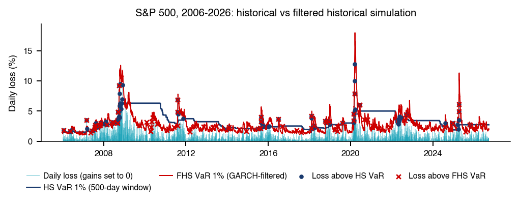

 MFM_ch7_loss_distribution
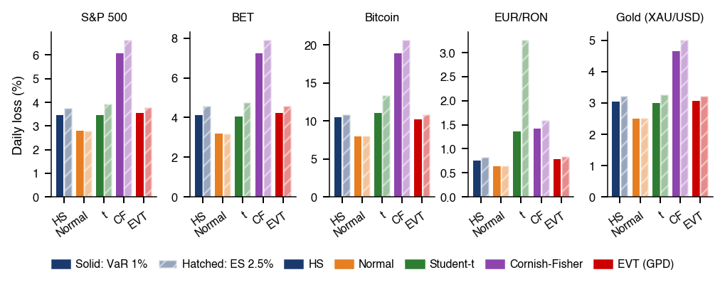
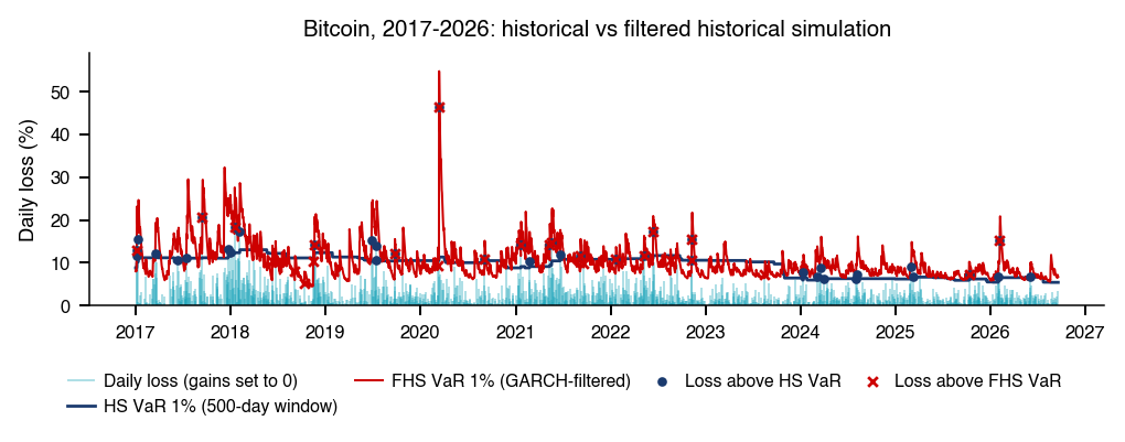

 Measuring Statistical Risk