Bucharest University of Economic Studies IDA Institute Digital Assets Blockchain Research Center AI4EFin Artificial Intelligence for Energy Finance Romanian Academy, Institute for Economic Forecasting MSCA Digital Finance
Since all models are wrong the scientist must be alert to what is importantly wrong. It is inappropriate to be concerned about mice when there are tigers abroad.
Chapters 2, 3 and 5 showed that the Normal distribution does not describe daily returns, and that the Student-t distribution, the stable laws and extreme value theory each capture part of what it misses. A risk manager therefore faces a practical choice among several heavy-tailed candidates, and the choice matters: the candidates agree near the centre of the distribution and differ by orders of magnitude in the tails, which is exactly where Value at Risk (VaR) and expected shortfall (ES) are read.
The data of the chapter make the stakes concrete. Fitted to daily S&P 500 returns since 2000, the Normal model puts the VaR 1% at 2.80%, against an empirical value of 3.45%, while the stable law puts it at 4.54%. Across seven series (three indices, Bitcoin and three Bucharest stocks), the Normal VaR 1% is between 14% and 24% too low, and no single distribution wins everywhere: the normal inverse Gaussian (NIG) law is best for the indices, the generalised error distribution (GED) for Bitcoin and the Student-t family for the stocks.
The chapter builds the toolbox for this choice: maximum likelihood, likelihood-ratio and Vuong tests, the information criteria AIC and BIC, goodness-of-fit tests and PP and QQ plots. It then judges the candidates by the purpose they serve, the VaR 1% in sample and out of sample, and ends with overfitting and with model uncertainty, the spread of the risk number across models that fit the data about equally well.
VaR 1% of six fitted models divided by the empirical VaR 1%, for BET, S&P 500, DAX, Bitcoin and three Bucharest stocks (TLV, SNP, BRD); daily log returns since 2000 (Bitcoin since 2014, the stocks since 2010). The dashed line at 1 marks a model that matches the data.
Learning outcomes
Write the log-likelihood of a candidate model and explain how maximum likelihood estimates are found.
Test a restricted model against a larger one with the likelihood-ratio test, and recognise when the test does not apply.
Compute AIC, BIC, ΔAIC and Akaike weights and interpret them.
Run and read the KS, Cramér–von Mises and Anderson–Darling tests and PP and QQ plots, and explain why KS is weak in the tails.
Judge a model by its VaR 1% out of sample, recognise overfitting and report model uncertainty.
Seminar 6 comes before this lecture and practises the same tools on data.
Chapter plan
Candidate DistributionsSeven distributions for daily returns, their tails, and the statistics every model must reproduce.
Review of Maximum Likelihood EstimationThe log-likelihood, the Normal case in closed form, numerical fits, the profile likelihood of ν and numerical problems.
SummaryKey ideas, key formulas and self-check questions.
Candidate Distributions
A statistical model of returns is chosen from a list of candidates, and the list itself is the first modelling decision. This section presents seven distributions used in the literature for daily returns, shows how differently they treat large losses although they look alike near the centre, and fixes the empirical facts that any candidate must reproduce: skewness, excess kurtosis and the occasional data error that can masquerade as a market crash.
The statistician George Box argued that the aim of modelling is a useful description, not a true one (Box, 1976). Every distribution fitted to returns is a simplification: returns are not independent, their volatility changes over time and their law drifts with market regimes. The phrase "all models are wrong, but some are useful" condenses his argument, and the epigraph of this page gives his own wording: the scientist must be alert to what is importantly wrong.
For returns, what is importantly wrong depends on the purpose. Pricing and portfolio choice depend mostly on the body of the distribution, the typical days that make up most of the sample. Risk management depends on the left tail, the worst 1% of days, which contains few observations but drives capital requirements, margins and losses. A model can describe the body well and the tail badly, and the reverse.
The chapter therefore has two goals. The first is a toolbox for comparing models: likelihood-based tests, information criteria, goodness-of-fit tests and plots. The second is a habit: before ranking models, ask what the model will be used for, and judge it on that use.
In brief
George Box: a statistician should look for a model that is useful, not one that is true Box (1976)
“all models are wrong, but some are useful” is the short form of his argument
For returns, “useful” depends on the purpose
pricing and portfolio choice: the body of the distribution (typical days)
risk management: the left tail (the worst 1% of days)
This chapter: a toolbox to compare models, and the habit of asking “useful for what?”
The table lists the seven candidates with their number of parameters \(k\), the shape of their tails and whether they allow skewness. The Normal distribution has thin tails that decay like \(e^{-x^2/2}\). The Student-t has power tails, with density decaying like a power of \(x\) governed by the degrees of freedom \(\nu\); the skewed-t of Hansen (1994) adds a skewness parameter \(\lambda\). The generalised error distribution (GED), used by Nelson (1991), has tails like \(e^{-|x|^\beta}\), which are heavier than Normal when \(\beta < 2\).
The Normal mixture of Kon (1984) draws each day from one of two Normal laws: with probability \(w\) a calm-day law \(N(\mu_1, \sigma_1^2)\), otherwise a turbulent-day law \(N(\mu_2, \sigma_2^2)\). Each component has thin tails, but the wide component produces many more large moves than a single Normal law with the same variance. The normal inverse Gaussian (NIG) distribution of Barndorff-Nielsen (1997) belongs to the generalised hyperbolic family studied for finance by Eberlein & Keller (1995); its tails are semi-heavy, a power factor times an exponential decay.
The stable laws of Chapter 3 have power tails with index \(\alpha < 2\), the heaviest of the list, and infinite variance. The candidates differ in their number of parameters, from 2 for the Normal law to 5 for the two-component mixture, and this count will matter when models are compared: a model with more parameters can always fit the same sample at least as well.
\(k\): number of parameters; GED: generalised error distribution; NIG: normal inverse Gaussian, a member of the generalised hyperbolic family Eberlein & Keller (1995)
Normal mixture: with probability \(w\) a calm-day \(N(\mu_1, \sigma_1^2)\), otherwise a turbulent-day \(N(\mu_2, \sigma_2^2)\)
Question for the room At x = 4, the Student-t distribution (ν = 4) gives a probability P(X < −4) 76 times that of the Normal distribution. The ▶ button moves the threshold from 2 to 6. How many times larger is the Student-t probability at x = 6?
Answer
About 536,000 times: 5.3 × 10⁻⁴ against 9.9 × 10⁻¹⁰. At x = 2 the two probabilities are almost equal (ratio 1.0), at x = 3 the ratio is 4.9, at x = 5 it is 3,682. The Normal tail falls as e−x²/2, the Student-t tail as a power of x, so the ratio grows ever faster with the threshold. The mean and the variance are the same; the difference lies only in the tail, where VaR 1% sits.
The chart draws one member of each family, all standardised to mean 0 and variance 1; the stable law, which has no variance, is scaled to the same interquartile range as the Normal law. The left panel shows the densities on a linear scale, the right panel the same densities on a logarithmic vertical scale, which makes the tails visible.
On the linear scale the curves are close: the heavy-tailed laws have a higher, narrower peak than the Normal density and slightly thinner shoulders, which is how a distribution with the same variance compensates for its larger tails. On the log scale the picture changes. Four standard deviations from the centre, the Normal density already lies below all the others, and beyond five standard deviations it falls below \(10^{-7}\), while the heavy-tailed densities stay between about \(10^{-6}\) and \(10^{-3}\).
This is the central difficulty of model selection for risk. Most observations lie near the centre, where the candidates agree, so the data contain little information to separate them, while the quantity of interest lies in the tail, where they disagree most.
In brief
All with mean 0 and variance 1 (stable: the same interquartile range as the Normal law); right panel on a log scale
Near the centre they look alike; in the tails they differ by orders of magnitude
The probability \(P(X < -4)\) of a fall of four standard deviations quantifies the tail disagreement for the members drawn in the chart. Under the Normal law it is \(3.2 \times 10^{-5}\), about one day in 31,000 trading days. Under the heavy-tailed candidates it ranges from \(9.5 \times 10^{-4}\) for the GED through \(2.4 \times 10^{-3}\) for the Student-t, \(2.5 \times 10^{-3}\) for the Normal mixture, \(3.2 \times 10^{-3}\) for NIG and \(4.5 \times 10^{-3}\) for the skewed-t, to \(8.1 \times 10^{-3}\) for the stable law.
The Student-t therefore assigns this loss a probability about 76 times the Normal one, although both distributions have the same variance. A risk measure such as the VaR 1% lies in exactly this region, so the choice of model translates directly into the size of the reported risk.
Question for the room: if all the candidates fit the centre well, why not keep the simplest one? Answer: the simplest one, the Normal law, is wrong precisely in the region that determines capital and margin requirements. A model that is good for typical days can be useless for the days that matter for risk.
In brief
\(P(X < -4)\), a move of four standard deviations, under each candidate of the chart:
Normal \(3.2 \times 10^{-5}\); GED \(9.5 \times 10^{-4}\); Student-t \(2.4 \times 10^{-3}\); Normal mixture \(2.5 \times 10^{-3}\)
Question for the room Without the two erroneous days of May 2016, the kurtosis of the TLV daily returns is 16.5. What does it become if the two days, −15.0% and +20.5%, stay in the data?
Answer
20.5. Kurtosis uses the fourth power of the deviations from the mean, so two extreme days move it a lot, even though their sum, +5.5%, is small. The skewness moves from −0.87 to −0.58. In the lecture, ν̂ of the Student-t falls from 3.44 to 3.33, and the AIC ranking does not change (Student-t wins in both cases). The JB of TLV rises too, because (K − 3)² rises.
Question for the room The kurtosis of the DAX monthly returns is 4.60 on the SFESumm sample (July 2004 – May 2014) and 5.06 on 2004–2026. The ▶ button extends the sample one year at a time. Does the kurtosis rise gradually as years are added?
Answer
No. Between 2014 and 2019 it falls, to 4.30 in May 2016, because the months added are calm. It jumps to 4.93 when the return from early March to early April 2020 enters, −21.70%, the new minimum of the sample (the old one was −19.35%). The kurtosis depends on a few extreme months, not on the number of months. On 2004–2026 the skewness stays negative (−0.72), and the Jarque–Bera test rejects Normality with JB = 70.2.
Before fitting any model, the data must be described. The chart shows monthly DAX log returns, computed between the first trading days of consecutive months. The darker segment is the sample of the classic SFESumm Quantlet of the textbook Franke, Härdle & Hafner (2019), July 2004 to May 2014 with \(n = 119\) months; the lighter segment extends the series to September 2026.
The series shows the features that motivate the chapter. Large negative months cluster in crises: late 2008, the summer of 2011 and March 2020, the worst month of the extended sample at about −21.7%. Positive months are more frequent but smaller, so the distribution is skewed to the left.
Monthly returns aggregate about twenty daily returns, so a central limit argument would suggest that they are closer to Normal than daily returns. The next frame shows that even at this frequency the Normal law is rejected.
In brief
Quantlet SFESumm: DAX monthly log returns between first trading days, July 2004 – May 2014 (\(n = 119\)), extended here to 1 Sep 2026
Even monthly returns are skewed and heavy-tailed: the next slide gives the numbers
The table reports, for monthly DAX log returns in percent, the minimum, the maximum, the standard deviation \(\sigma\), the annualised volatility \(\sigma\sqrt{12}\), the skewness \(E(X-\mu)^3/\sigma^3\) and the kurtosis \(E(X-\mu)^4/\sigma^4\), where \(\mu\) is the mean; the Normal law has skewness 0 and kurtosis 3. In the SFESumm sample, 2004–2014, the monthly standard deviation is 5.80% (annualised 20.08%), the skewness −0.83 and the kurtosis 4.60. Over 2004–2026 (\(n = 267\) months) the standard deviation is 5.39% (annualised 18.66%), the skewness −0.72 and the kurtosis 5.06. The Jarque–Bera test of Chapter 2 rejects Normality in both samples with a \(p\)-value below 0.001.
Daily returns depart much further from the Normal law. Since 2000 (Bitcoin since 2014, the Bucharest stocks since 2010), the kurtosis of daily log returns is 14.1 for the BET, 13.7 for the S&P 500, 9.1 for the DAX, 15.0 for Bitcoin, 16.5 for Banca Transilvania (TLV), 11.9 for OMV Petrom (SNP) and 10.3 for BRD. The skewness is −0.35 for the S&P 500, −0.65 for the BET and −0.70 for Bitcoin.
These are the targets for the candidates: a model for daily returns must produce kurtosis far above 3 and, for some series, a longer left tail. A candidate list chosen for convenience rather than for these facts would decide the outcome before any test is run.
In brief
\(n\)
min
max
st. dev.
ann. vol.
skew.
kurt.
DAX 2004–2014
119
\(-19.35\)
\(17.12\)
\(5.80\)
\(20.08\)
\(-0.83\)
\(4.60\)
DAX 2004–2026
267
\(-21.70\)
\(17.12\)
\(5.39\)
\(18.66\)
\(-0.72\)
\(5.06\)
Monthly, in %; st. dev.: standard deviation \(\sigma\); ann. vol.: \(\sigma\sqrt{12}\)
skewness \(E(X - \mu)^3/\sigma^3\) and kurtosis \(E(X - \mu)^4/\sigma^4\), with \(\mu\) the mean; 0 and 3 for the Normal distribution
Jarque–Bera test of Normality (Chapter 2): \(p\)-value \(<0.001\)
Daily log returns since 2000 (Bitcoin since 2014, BVB stocks since 2010): kurtosis
BET \(14.1\), S&P 500 \(13.7\), DAX \(9.1\), Bitcoin \(15.0\), TLV \(16.5\), SNP \(11.9\), BRD \(10.3\)
skewness: S&P 500 \(-0.35\), BET \(-0.65\), Bitcoin \(-0.70\)
Extreme observations dominate tail estimates, so an error in one of them can change the fitted model. The adjusted close of Banca Transilvania (TLV) from the data provider EODHD shows a log return of −15.0% on 30 May 2016 followed by +20.5% on 31 May 2016. As explained in Chapter 2, the adjustment for a distribution of bonus shares is applied one day late, which creates a fake crash followed by a fake rally.
The two days change the moments noticeably. With them the kurtosis of daily TLV returns is 20.5, without them 16.5, and the fitted Student-t degrees of freedom \(\hat\nu\) move from 3.33 to 3.44. Here the ranking of the models by AIC is unchanged (the Student-t is best in both cases), but in a smaller sample or for a quantity defined by the tail, two wrong days could change the conclusion.
The rule that follows is to check the largest returns against the closing prices and the news before any model selection, and to remove only errors that are proven. In the rest of the chapter, the two TLV days are removed.
In brief
Banca Transilvania (TLV), adjusted close from EODHD: log returns of \(-15.0\%\) on 30 May 2016 and \(20.5\%\) on 31 May 2016
the adjustment for the bonus shares is applied one day late (Chapter 2): a fake crash followed by a fake rally
Effect of the two days on the fitted model
kurtosis \(20.5\) with them, \(16.5\) without; Student-t \(\hat\nu\): \(3.33\) vs \(3.44\)
the AIC ranking does not change here (best: Student-t), but the moments do
Rule: check the largest returns against the close and the news before any model selection; the two days are removed in the rest of the chapter
Section summary
The seven candidates span thin, semi-heavy and power tails, with 2 to 5 parameters, and they agree near the centre while differing by orders of magnitude in the tail. Daily returns have kurtosis between 9 and 17 and, for several series, negative skewness, and clean data are a precondition for any comparison. The next section recalls the estimation method that turns each candidate into a fitted model.
Review of Maximum Likelihood Estimation
Every comparison in this chapter starts from the maximised log-likelihood of each candidate. This section recalls the likelihood principle, works through the Normal model in closed form, reports the numerical fits of the other six candidates for the S&P 500 and interprets their parameters. It ends with the precision of the tail parameter, measured by the profile log-likelihood, and with the numerical problems of the optimisation.
Let \(r_1, \dots, r_n\) be daily returns, assumed independent and identically distributed (i.i.d.) with density \(f(r; \theta)\), where \(\theta\) is the vector of model parameters, for example \((\mu, \sigma)\) for the Normal model. The likelihood \(L(\theta) = \prod_t f(r_t; \theta)\) is the joint density of the observed sample, read as a function of \(\theta\). Because products of many small numbers are numerically awkward and sums are easier to differentiate, one works with the log-likelihood
The maximum likelihood (ML) estimate is the parameter value that makes the observed data most probable, \(\hat\theta = \arg\max_\theta \ell(\theta)\). The maximised value \(\ell(\hat\theta)\) measures how well the best member of a family describes the data, and it is the raw material of the likelihood-ratio test, the Vuong test and the information criteria later in the chapter.
For large \(n\), under regularity conditions, \(\hat\theta\) is approximately Normal around the true \(\theta\), with covariance approximated by the inverse of the observed information, \([-\partial^2\ell/\partial\theta\,\partial\theta^\top]^{-1}\). The second derivative measures the curvature of \(\ell\) at its maximum: a sharply curved log-likelihood means that small changes of \(\theta\) lower the fit a lot, so the data pin the parameter down precisely.
In brief
Data \(r_1, \dots, r_n\), assumed i.i.d. (independent, identically distributed) with density \(f(r; \theta)\)
\(\theta\): the vector of model parameters (for example \(\mu, \sigma\)); \(f\): the density of the model
likelihood: \(L(\theta) = \prod_{t=1}^n f(r_t; \theta)\), the probability density of the observed sample as a function of \(\theta\)
log-likelihood: \(\ell(\theta) = \sum_{t=1}^n \ln f(r_t; \theta)\); sums are easier than products
Maximum likelihood (ML) estimate: \(\hat\theta = \arg\max_\theta \ell(\theta)\)
\(\ell(\hat\theta)\), the maximised log-likelihood, is the raw material of every comparison in this chapter
Large \(n\): \(\hat\theta\) is approximately Normal around the true \(\theta\)
covariance \(\approx [-\partial^2\ell/\partial\theta\,\partial\theta^\top]^{-1}\), the inverse of the observed information
a sharply curved \(\ell\) (large second derivative) means a precise estimate
Setting the derivatives with respect to \(\mu\) and \(\sigma^2\) to zero gives \(\hat\mu = \bar r\) and \(\hat\sigma^2 = \frac{1}{n}\sum_t (r_t - \bar r)^2\), the sample variance with divisor \(n\) rather than \(n - 1\). Substituting back, the sum of squares equals \(n\hat\sigma^2\), and the maximised log-likelihood takes the compact form \(\ell(\hat\theta) = -\frac{n}{2}[\ln(2\pi\hat\sigma^2) + 1]\).
For daily S&P 500 log returns in percent from 2000 to 2026, \(n = 6\,714\), the mean is \(\hat\mu = 0.025\) and the standard deviation \(\hat\sigma = 1.213\). Then \(\ln(2\pi\hat\sigma^2) = 2.2240\) and \(\ell(\hat\theta) = -\frac{6714}{2}(2.2240 + 1) = -10\,823\). The number has no meaning on its own; it becomes informative when compared with the maximised log-likelihood of another model on the same data.
The Normal model is the only candidate with a closed-form solution. For the other six, the log-likelihood has to be maximised numerically.
The table reports the ML estimates and the maximised log-likelihoods of the seven candidates for the S&P 500. The Normal model reaches −10,823; every heavy-tailed candidate does much better, from −9,925 for the Normal mixture to −9,824 for NIG, the highest value. The Student-t reaches −9,848, the skewed-t −9,838, the GED −9,854 and the stable law −9,893. Differences of tens or hundreds of log-likelihood points are very large: a difference of 10 means that the data are \(e^{10} \approx 22\,000\) times more likely under one fitted model than under the other.
The optimiser is the Nelder–Mead simplex method applied to transformed parameters, such as \(\ln\sigma\) for a scale or \(\ln(\nu - 2)\) for the degrees of freedom, so that the search runs over an unconstrained space and every candidate value is admissible. The Normal mixture is fitted with the expectation–maximisation (EM) algorithm, which alternates between assigning each day a probability of belonging to each component and re-estimating the components. The stable density has no closed form and is computed by the fast Fourier transform (FFT) of its characteristic function, as in Chapter 3.
Parameters must be read in the parameterisation used. In Hansen's skewed-t, \(\mu\) and \(\sigma\) are the mean and the standard deviation, so \(\hat\sigma = 1.39\) is directly comparable with the Normal \(\hat\sigma = 1.213\); in the Student-t and the GED, "scale" is a scale parameter, not the standard deviation.
Optimiser: Nelder–Mead on transformed parameters (for example \(\ln\sigma\), \(\ln(\nu - 2)\)); the Normal mixture by the EM (expectation–maximisation) algorithm; the stable density by FFT (Chapter 3)
Skewed-t: \(\mu\) and \(\sigma\) are the mean and the standard deviation (Hansen's parameterisation)
The Student-t estimate \(\hat\nu = 2.67\) means that the density tails decay like a power of \(x\) with exponent governed by \(\nu\), so that moments of order below 2.67 exist and higher ones do not. The variance is finite (\(\nu > 2\)), but the kurtosis is not (\(\nu < 4\)). The sample kurtosis of 13.7 is then an estimate of a quantity that the fitted model declares infinite, which explains why sample kurtosis values of daily returns are unstable and dominated by a few extreme days.
The skewed-t estimate \(\hat\lambda = -0.067\) is negative, which means a slightly longer left tail: large falls are a little more likely than large rises of the same size. The GED estimate \(\hat\beta = 0.88\) lies below 2, the Normal case, and even below 1, the Laplace case, which corresponds to a sharp peak and tails heavier than exponential.
The Normal mixture splits the days into 79% calm days with standard deviation 0.71% and 21% turbulent days with standard deviation 2.26% and a negative mean of −0.223%, a reading in terms of market regimes. The stable law has \(\hat\alpha = 1.540\), well below 2, which gives it heavier tails than any other candidate.
In brief
Student-t \(\hat\nu = 2.67\): tails like \(x^{-2.67}\); the variance exists (\(\nu > 2\)), the kurtosis does not (\(\nu < 4\))
the sample kurtosis \(13.7\) estimates a quantity that the fitted model says is infinite
Skewed-t \(\hat\lambda = -0.067 < 0\): a slightly longer left tail (crashes)
GED \(\hat\beta = 0.88\): below 2 (Normal) and even below 1 (Laplace): a sharp peak
Normal mixture: \(79\%\) calm days with standard deviation \(0.71\%\), \(21\%\) turbulent days with \(2.26\%\) and a negative mean
Stable \(\hat\alpha = 1.540\) (Chapter 3): heavier tails than any other candidate
Precision of \(\hat\nu\): the Profile Log-Likelihood
Question for the room For the S&P 500, ν̂ of the Student-t distribution is 2.67. Bitcoin has a larger sample kurtosis (15.0 against 13.7). Is the ν̂ of Bitcoin smaller or larger?
Answer
Smaller: 2.23, the smallest of the seven series, hence the heaviest tail. BET has 2.43, DAX 3.09, BRD 4.67. A ν̂ close to 2 means a variance that is barely finite. The large standard deviation of Bitcoin (3.5% per day) goes into the scale, not into ν: the Student-t scale of Bitcoin is 1.85, and the implied standard deviation, scale·√(ν/(ν − 2)), is 5.75%, above the sample standard deviation (3.49%), because ν̂ is close to 2.
Question for the room For BRD, the test of Student-t inside skewed-t (λ = 0) gives LR = 3.01. Is the skewness parameter needed at 5%?
Answer
No: 3.01 < 3.84, p = 0.083. The fixed value λ = 0 lies inside the interval (−1, 1), so Wilks' theorem applies and the critical value is 3.84; 2.71 is the boundary value (Normal inside Student-t). AIC still prefers skewed-t (ΔAIC of Student-t: 1.0), because AIC is not a test: it charges 2 for a parameter, and LR > 2. The skewness is significant only for the S&P 500 (LR = 19.63) and the DAX (20.92).
The statistic V and its p-value on the seven series
Cumulative sum of the daily differences mt
Question for the room On the slide, Student-t is preferred to the stable distribution on all four markets. For BRD, V = 1.89. Is the preference significant at 5%?
Answer
No: |V| = 1.89 < 1.96, p = 0.059. Student-t explains the BRD days better on average, but the difference is not separated from noise. The day with the largest |mt| is 19 December 2018 (mt = −2.48: the stable distribution explains this fall better). For TLV and SNP, V = 3.77 and 4.16. The sum of the daily differences is exactly the difference of the log-likelihoods, ℓ(Student-t) − ℓ(stable).
Question for the room The slide gives the 95% interval for ν of the S&P 500, [2.47, 2.89], where the profile crosses the cut-off. Which points of the grid of step 0.1 used in the chart lie inside the interval?
Answer
From 2.5 to 2.8. The true end points, 2.47 and 2.89, lie between grid points (2.4–2.5 and 2.8–2.9); a 0.1 grid read directly would give [2.5, 2.8], an interval that is too narrow. The interval is not symmetric around ν̂ = 2.67: 0.20 to the left, 0.22 to the right, because the profile is not a parabola. At ν = 5, the profile log-likelihood is 92.3 below its maximum.
The precision of \(\hat\nu\) can be read from the profile log-likelihood. For each fixed value of \(\nu\) on a grid, \(\ell\) is maximised over the location and scale, and the chart plots the result minus its overall maximum, \(\ell(\nu) - \ell(\hat\nu)\). The curve peaks at \(\hat\nu = 2.67\) (dotted line) and falls steeply on both sides; at \(\nu = 5\) it lies 92 points below the maximum.
By the likelihood-ratio argument of the next section, a 95% confidence interval for \(\nu\) contains every value with \(2[\ell(\hat\nu) - \ell(\nu)] \le 3.84\), the 95% quantile of the \(\chi^2(1)\) distribution, that is, every \(\nu\) whose profile lies above the dashed line at \(-3.84/2 = -1.92\). The profile crosses the dashed line at \(\nu = 2.47\) and \(\nu = 2.89\), so the interval is \([2.47, 2.89]\); on the grid of step 0.1 used for the chart, the points inside run from 2.5 to 2.8.
The narrow interval says that the tail index of the S&P 500 is pinned down well by 6,714 daily returns. A Student-t with 5 degrees of freedom, a value often used as a default, is firmly rejected for this series. The profile likelihood is preferable to the symmetric interval built from the standard error when the log-likelihood is asymmetric around its maximum, as it is here.
In brief
For each \(\nu\), maximise \(\ell\) over location and scale; at \(\nu = 5\) the curve is \(92\) below its maximum
95% interval: all \(\nu\) with \(2[\ell(\hat\nu) - \ell(\nu)] \le 3.84\), here \([2.47, 2.89]\) around \(\hat\nu = 2.67\): the tails are pinned down well
Numerical maximisation can fail in ways that produce wrong numbers without any error message. The first risk is a local maximum: the optimiser climbs the nearest hill and stops, even if a higher one exists elsewhere. Mixtures are especially prone to this, because components can be swapped or merged; the remedy is to start from several initial values and keep the best result, and the mixtures in this chapter use between 4 and 12 starting points.
The second risk is the boundary of the parameter space: \(\nu \to 2\) in the Student-t, where the variance becomes infinite, a mixture weight going to 0, or \(|\lambda| \to 1\) in the skewed-t. At a boundary the usual standard errors and the usual distribution of test statistics are no longer valid, a problem the next section treats in detail. The third risk is the parameterisation: the same law can be written with different parameters, and software defaults differ. In scipy, for example, the Student-t scale is not the standard deviation, which equals \(\mathrm{scale}\sqrt{\nu/(\nu - 2)}\).
A simple consistency check catches many errors: when one model contains another as a special case, its maximised log-likelihood can never be lower. If the skewed-t reports a lower \(\ell(\hat\theta)\) than the Student-t on the same data, the optimiser has failed.
In brief
Local maxima: the optimiser can stop on a hill that is not the highest
remedy: several starting values (the mixtures in this chapter use 4 to 12 starts)
the usual standard errors and tests are not valid at a boundary (next section)
Parameterisation: the same law, different parameters
scipy's Student-t scale is not the standard deviation: \(\mathrm{sd} = \mathrm{scale}\sqrt{\nu/(\nu - 2)}\)
Check: compare \(\ell(\hat\theta)\) of nested models; a larger model can never have a lower maximum
Section summary
Maximum likelihood turns each candidate into a fitted model and a single number, \(\ell(\hat\theta)\). For the S&P 500 every heavy-tailed model improves on the Normal log-likelihood by roughly 900 to 1,000 points, NIG reaches the highest value, and the Student-t tail index is estimated at 2.67 with a 95% interval of \([2.5, 2.8]\).The next section asks when a gain in log-likelihood is larger than chance.
Nested Models: the Likelihood-Ratio Test
A larger model always fits at least as well as a model it contains. The likelihood-ratio test decides whether the gain is larger than sampling noise would produce. This section defines nested models, states Wilks' theorem, applies the test to the skewness parameter and to the Normal law inside the GED, treats the boundary case of the Normal law inside the Student-t and introduces the Vuong test for models that are not nested.
Model 0 is nested in model 1 if model 0 is obtained from model 1 by fixing some of its parameters. The Normal law is the GED with \(\beta = 2\); the Student-t is the skewed-t with \(\lambda = 0\); the Normal law is the limit of the Student-t as \(\nu \to \infty\), that is, the value \(1/\nu = 0\). The last case is special because \(1/\nu = 0\) lies on the edge of the admissible region \(1/\nu \ge 0\), not inside it.
Many pairs of candidates are not nested: the Student-t and the GED, the Student-t and the stable law, the skewed-t and NIG. Neither member of such a pair is a special case of the other, so a test built on restrictions cannot compare them, and other tools are needed: the Vuong test at the end of this section and the information criteria of the next one.
For nested models, \(\ell_1(\hat\theta_1) \ge \ell_0(\hat\theta_0)\) always holds, because the larger model can reproduce the smaller one by choosing the restricted values. The statistical question is therefore not whether the larger model fits better, but whether the improvement is larger than what the extra parameters would achieve by fitting noise.
In brief
Model 0 is nested in model 1 if model 0 is model 1 with some parameters fixed
Normal inside GED: \(\beta = 2\)
Student-t inside skewed-t: \(\lambda = 0\)
Normal inside Student-t: \(\nu = \infty\), i.e. \(1/\nu = 0\), on the edge of the parameter space
Not nested: Student-t and GED, Student-t and stable, skewed-t and NIG
neither is a special case of the other: they need other tools (Vuong test, AIC)
Nested: \(\ell_1(\hat\theta_1) \ge \ell_0(\hat\theta_0)\) always; the question is whether the gain is larger than chance
The null hypothesis \(H_0\) states that the restricted model 0 is true; the alternative \(H_1\) is the larger model 1. With \(\ell_0\) and \(\ell_1\) the maximised log-likelihoods and \(k_0 < k_1\) the numbers of parameters, the likelihood-ratio statistic is twice the gain in maximised log-likelihood:
Since \(\ell\) is a logarithm, \(LR\) is twice the log of how many times more probable the data are under the fitted larger model. Wilks' theorem (Wilks, 1938) gives its distribution under \(H_0\): for large \(n\),\(LR\) is approximately chi-square with \(d = k_1 - k_0\) degrees of freedom, the number of restrictions. The theorem requires the restricted values to lie inside the parameter space.
At the 5% level, \(H_0\) is rejected when \(LR\) exceeds the 95% quantile \(\chi^2_{0.95}(d)\), which is 3.84 for one restriction and 5.99 for two. These thresholds are low compared with the log-likelihood differences of the previous section, which already suggests that many of the restrictions will be rejected on daily data.
In brief
\(H_0\): model 0 (restricted) is true; \(H_1\): model 1 (larger)
\(LR = 2\,[\ell_1(\hat\theta_1) - \ell_0(\hat\theta_0)] \ge 0\): twice the gain in maximised log-likelihood
\(\ell_0, \ell_1\): the log-likelihoods of the two models; \(k_0, k_1\): their numbers of parameters
Wilks' theorem (Wilks (1938)): under \(H_0\), \(LR \approx \chi^2(d)\), with \(d = k_1 - k_0\) restrictions
\(\chi^2(d)\): the chi-square distribution with \(d\) degrees of freedom
valid if the restricted values are inside the parameter space
Decision at 5%: reject \(H_0\) if \(LR > \chi^2_{0.95}(d)\)
For the S&P 500 the Student-t reaches \(\ell = -9\,848\) and the skewed-t \(\ell = -9\,838\). The skewed-t has one parameter more, so \(d = 1\). From the unrounded log-likelihoods, \(LR = 19.63\), far above 3.84, with a \(p\)-value below 0.001: the restriction \(\lambda = 0\) is rejected, and the S&P 500 needs a skewness parameter. The DAX gives the same answer, with \(LR = 20.92\) and \(p < 0.001\).
The BET and Bitcoin give the opposite answer. For the BET, \(LR = 0.35\) with \(p = 0.555\); for Bitcoin, \(LR = 0.42\) with \(p = 0.515\). In both, the skewed-t does not fit significantly better than the symmetric Student-t, so the data offer no evidence of tail asymmetry once heavy tails are allowed. The sample skewness of −0.65 for the BET and −0.70 for Bitcoin is then explained by a few extreme days rather than by a systematically longer left tail.
The test of the Normal law inside the GED (\(\beta = 2\)) gives \(LR\) values between 1,431 for Bitcoin and 2,298 for the BET: the Normal model is rejected for every series by a huge margin. The interpretation is that the two developed-market indices have a longer left tail, while the BET and Bitcoin have heavy but roughly symmetric tails.
Testing the Normal law against the Student-t means testing \(H_0: 1/\nu = 0\). This value lies on the edge of the parameter space \(1/\nu \ge 0\), and Wilks' theorem does not apply, because the estimate can only fall on one side of the null value. Self & Liang (1987) showed that the null distribution of \(LR\) is then a 50:50 mixture of \(\chi^2(0)\), a point mass at 0, and \(\chi^2(1)\): in half of the samples the best fit is the Normal law itself and \(LR = 0\).
The 5% critical value becomes the 90% quantile of \(\chi^2(1)\),\(\chi^2_{0.90}(1) = 2.71\), instead of 3.84, and the naive \(p\)-value from \(\chi^2(1)\) is twice the correct one. The same issue arises whenever the null sets a parameter at the edge of its range, for example a mixture weight \(w = 0\) or a variance equal to 0.
On real data the boundary has no practical effect: \(LR = 1\,949\) for the S&P 500 and \(1\,337\) for Bitcoin, so the Normal law is rejected under either critical value. What do you think? Does the boundary matter when \(LR\) is in the thousands? Answer: not for this decision; it matters in small samples and for borderline values of \(LR\), where it halves the \(p\)-value and can turn a non-rejection into a rejection.
In brief
\(H_0\): \(1/\nu = 0\) is on the edge of the space \(1/\nu \ge 0\): Wilks' theorem does not apply
Self & Liang (1987): the null law is a 50:50 mixture of \(\chi^2(0)\) (a point mass at 0) and \(\chi^2(1)\)
5% critical value: \(\chi^2_{0.90}(1) = 2.71\) instead of \(3.84\); the naive \(p\)-value is twice the correct one
Real data: \(LR\) = 1 949 (S&P 500), 1 337 (Bitcoin): the Normal model is rejected with either critical value
The same issue appears for a mixture weight \(w = 0\) and for variance parameters equal to 0
What do you think? Does the boundary matter when \(LR\) is in the thousands?
Answer
no for the decision; yes for small samples and borderline \(LR\) values, where it halves the \(p\)-value
For non-nested models, Vuong (1989) compares the fitted densities day by day. For each day \(t\),\(m_t = \ln f_1(r_t) - \ln f_2(r_t)\) measures by how much model 1 explains that day better than model 2. With \(\bar m\) and \(s_m\) the mean and standard deviation of the \(m_t\), the statistic \(V = \sqrt{n}\,\bar m / s_m\) is approximately standard Normal if both models are equally close to the true distribution. \(V > 1.96\) favours the first model and \(V < -1.96\) the second at the 5% level; values in between do not separate them.
The table reports \(V\) with its \(p\)-value in brackets for three pairs and four series. The Student-t beats the stable law on every series, with \(V\) from 6.52 for the S&P 500 to 16.47 for Bitcoin. NIG beats the skewed-t on the S&P 500 (\(V = -2.20\),\(p = 0.028\)), the DAX (\(V = -2.97\),\(p = 0.003\)) and Bitcoin (\(V = -6.76\)), while for the BET the difference is not significant (\(V = -1.34\),\(p = 0.179\)).
The comparison of the Student-t with the GED splits by market. The Student-t is closer for the BET (\(V = 3.70\)), the GED is closer for Bitcoin (\(V = -3.80\)), and the two cannot be separated for the S&P 500 (\(V = 0.40\)) or the DAX (\(V = -0.23\)). The Vuong test thus gives a first sign of a result that the information criteria will confirm: the best model depends on the market.
In brief
Student-t vs GED
Student-t vs stable
skewed-t vs NIG
BET
\(3.70\) (\(<0.001\))
\(9.33\) (\(<0.001\))
\(-1.34\) (\(0.179\))
S&P 500
\(0.40\) (\(0.686\))
\(6.52\) (\(<0.001\))
\(-2.20\) (\(0.028\))
DAX
\(-0.23\) (\(0.817\))
\(7.66\) (\(<0.001\))
\(-2.97\) (\(0.003\))
Bitcoin
\(-3.80\) (\(<0.001\))
\(16.47\) (\(<0.001\))
\(-6.76\) (\(<0.001\))
Vuong (1989): \(m_t = \ln f_1(r_t) - \ln f_2(r_t)\), \(V = \sqrt{n}\,\bar m / s_m \approx N(0, 1)\) if both models are equally close to the truth
\(f_1, f_2\): the two fitted densities; \(m_t\): by how much model 1 explains day \(t\) better; \(\bar m\), \(s_m\): mean and standard deviation of the \(m_t\)
\(V > 1.96\): the first model is closer; \(V < -1.96\): the second; (\(p\)-value) in brackets
Student-t beats the stable law everywhere; NIG beats the skewed-t on the S&P 500 and the DAX; Student-t vs GED splits by market
The likelihood-ratio test compares nested models through twice the log-likelihood gain, referred to a \(\chi^2\) distribution with as many degrees of freedom as restrictions, provided the null lies inside the parameter space; at the boundary the critical value is halved in probability. The skewness parameter is needed for the S&P 500 and the DAX but not for the BET and Bitcoin, the Normal law is rejected everywhere, and the Vuong test ranks non-nested pairs differently across markets. The next section introduces criteria that rank all candidates at once.
Information Criteria: AIC and BIC
Tests compare two models at a time and answer a yes-or-no question. Information criteria rank any number of candidates, nested or not, on a common scale. This section presents Akaike's argument from the Kullback–Leibler divergence, defines AIC and BIC, introduces ΔAIC and Akaike weights, and applies them to the seven candidates on the S&P 500 and on six other series.
Akaike's Approach: the Kullback–Leibler Divergence
Hirotugu Akaike asked which model will predict new data best, rather than which model is true. He measured the distance from the true density \(g\) to a model \(f\) by the Kullback–Leibler divergence (Kullback & Leibler, 1951),
\[KL(g, f) = E_g[\ln g(R) - \ln f(R)] \ge 0,\]
where \(R\) is a new return drawn from \(g\) and \(E_g\) is the mean under \(g\). The divergence is zero only when \(f = g\). Since \(E_g \ln g(R)\) does not depend on the model, ranking models by KL is the same as ranking them by their expected log density on new data.
The maximised log-likelihood \(\ell(\hat\theta)\) is a natural estimate of that expected log density, but it is too optimistic, because the same data choose \(\hat\theta\) and then judge it. Akaike (1974) showed that the optimism is, on average, approximately \(k\), the number of estimated parameters. Subtracting \(k\) from \(\ell(\hat\theta)\) corrects the bias; multiplied by −2 to match the scale of the likelihood-ratio statistic, this becomes a penalty of 2 per parameter, which defines the criterion of the next frame.
In brief
Hirotugu Akaike asked: which model will predict new data best?
the distance from the truth \(g\) to a model \(f\): the Kullback–Leibler divergence Kullback & Leibler (1951)
\(KL(g, f) = E_g[\ln g(R) - \ln f(R)] \ge 0\), zero only if \(f = g\)
\(R\): a new return drawn from the truth \(g\); \(E_g\): the mean under \(g\)
\(\ell(\hat\theta)\) is too optimistic: the same data choose \(\hat\theta\) and judge it
the optimism is about \(k\), the number of parameters Akaike (1974)
Result: a penalty of 2 per parameter corrects the optimism; the criterion, AIC, is on the next slide
Both reward fit through \(-2\ell(\hat\theta)\) and penalise complexity through the number of parameters \(k\); for both, lower is better. AIC aims at the model with the best predictive performance; Stone (1977) showed that it is asymptotically equivalent to leave-one-out cross-validation. In small samples its bias correction is not enough, and the corrected version \(\mathrm{AICc} = \mathrm{AIC} + 2k(k+1)/(n - k - 1)\) of Hurvich & Tsai (1989) is preferred.
BIC aims at the true model, if it is among the candidates: it is consistent, choosing the true model with probability tending to 1 as \(n\) grows. Its penalty per parameter is \(\ln n\), which is 8.81 for the \(n = 6\,714\) daily S&P 500 returns, more than four times the AIC penalty of 2. BIC therefore favours smaller models than AIC, more strongly the longer the sample.
The absolute value of AIC or BIC has no meaning: it depends on the units of the data and on the sample size. Only differences between models fitted to the same data can be interpreted.
In brief
AIC (Akaike information criterion): \(\mathrm{AIC} = -2\ell(\hat\theta) + 2k\)
aim: the best predictive model; asymptotically equivalent to leave-one-out cross-validation Stone (1977)
The difference \(\Delta_i = \mathrm{AIC}_i - \min_j \mathrm{AIC}_j\) measures how far model \(i\) is from the best candidate. Burnham & Anderson (2004) give rules of thumb: models with \(\Delta \le 2\) have substantial support, models with \(4 \le \Delta \le 7\) considerably less, and models with \(\Delta > 10\) essentially none.
The differences can be turned into Akaike weights,
which sum to 1 and can be read as the weight of evidence for model \(i\) among the candidates considered. For two models with \(\Delta = 0\) and \(\Delta = 2\), the weights are \(1/(1 + e^{-1}) \approx 0.73\) and \(0.27\): the better model is favoured, but the other keeps more than a quarter of the weight.
What do you think? Is \(\Delta = 2\) a "significant" difference? Answer: no. AIC is not a test and has no significance level; a gap of 2 means that both models remain plausible, as the weights show. The weights are also relative to the candidate list: adding or removing a model changes all of them.
The table applies the criteria to the S&P 500. For NIG, with \(\ell(\hat\theta) = -9\,824\) and \(k = 4\),\(\mathrm{AIC} = -2(-9\,824) + 2 \cdot 4 = 19\,657\). NIG has the lowest AIC and the lowest BIC, so its ΔAIC and ΔBIC are both 0. The next model, the skewed-t, has \(\Delta\mathrm{AIC} = 28.1\), so \(e^{-\Delta/2} \approx 8.1 \times 10^{-7}\) and NIG receives an Akaike weight of practically 1.
The other candidates follow at larger distances: the Student-t at ΔAIC 45.7, the GED at 57.9, the stable law at 137.3, the Normal mixture at 202.5 and the Normal law at 1,993.2. By the rules of thumb, none of them has any support relative to NIG for this series.
The two criteria agree here because the log-likelihood differences are much larger than the penalties. Where they differ, BIC moves the small models closer to the leader: the Student-t, with 3 parameters, has ΔBIC 38.9 against ΔAIC 45.7, and the Normal law 1,979.6 against 1,993.2.
NIG wins on both criteria; the next model, skewed-t, has \(\Delta = 28.1\), so \(e^{-\Delta/2} \approx 8.1 \times 10^{-7}\): weight \(w \approx 1\) for NIG
Normal: \(\Delta\)AIC of 1 993; the stable law: 137
Question for the room For BRD, AIC prefers skewed-t, and Student-t has ΔAIC = 1.0. What Akaike weights do the two models get?
Answer
0.62 for skewed-t and 0.38 for Student-t (the other five models have weights of practically zero): w = e−Δ/2/Σ e−Δj/2, with e−0.5 = 0.61. A difference of 1 leaves both models plausible; AIC is not a test. With BIC weights the order reverses: 0.93 for Student-t.
Question for the room For BRD, AIC prefers skewed-t (ΔAIC of Student-t: 1.0). The ▶ button switches to BIC. Which model does BIC prefer?
Answer
Student-t, with ΔBIC = 5.2 for skewed-t. BIC charges the extra parameter ln 3,771 = 8.24, more than the gain in fit (LR = 3.01). For TLV and SNP, both criteria choose Student-t; for BET, S&P 500 and DAX, NIG; for Bitcoin, GED. The Normal model has ΔBIC between 472 and 2,412.
The heat map repeats the comparison for seven series: the BET, the S&P 500, the DAX, Bitcoin, and the Bucharest stocks Banca Transilvania (TLV), OMV Petrom (SNP) and BRD. Each row is a series, each column a candidate, and each cell shows ΔAIC; the value 0 marks the best model of the row. The colour scale is logarithmic in ΔAIC + 1, so that differences of 2 and of 2,000 are both visible.
Reading by columns, the Normal model is the darkest column for every series, with ΔAIC from 479 for BRD to 2,425 for the BET. Reading by rows, the white cell, the winner, moves: NIG for the three indices, the GED for Bitcoin, the Student-t for TLV and SNP, and the skewed-t for BRD.
For the Bucharest stocks several heavy-tailed models are close: the Student-t and the skewed-t are within 2 points of each other for all three stocks. For the indices, by contrast, the winner is clear, with the next model at least 14 points behind.
In brief
Each row: one series; 0 marks the best model; darker cells: worse models (log colour scale)
The first lesson of the map is that there is no single winner: the best distribution depends on the market. NIG wins for the indices, the GED for Bitcoin, and the Student-t family for the individual stocks. A risk system that applies the same distribution to every asset therefore accepts a worse fit for some of them.
Some conclusions are robust across all seven series. The Normal model is last everywhere, by 479 (BRD) to 2,425 (BET) AIC points. The stable law, with ΔAIC between 23 and 197, and the Normal mixture are never competitive: the stable tails are too heavy for daily returns, and two Normal components are not flexible enough.
Question for the room: for BRD, AIC prefers the skewed-t, with the Student-t only 1.0 point behind; which model does BIC prefer? Answer: the Student-t. Dropping one parameter saves \(\ln n \approx 8.2\) BIC points for the BRD sample, more than the gain in fit from the skewness parameter. With a difference of about 1, the two models are practically tied, and the choice between them matters less than the choice between them and the Normal law.
In brief
No single winner: the best model depends on the market
indices (BET, S&P 500, DAX): NIG; Bitcoin: GED; BVB stocks: Student-t (TLV, SNP) and skewed-t (BRD)
Robust conclusions
the Normal model is last everywhere, by 479 (BRD) to 2 425 (BET) points
the stable law (\(\Delta\) from 23 to 197) and the Normal mixture are never competitive
Question for the room: for BRD, AIC prefers the skewed-t (\(\Delta\) of the Student-t: \(1.0\)); which model does BIC prefer?
Answer
the Student-t: one parameter less saves \(\ln n \approx 8.2\) BIC points, more than the gain in fit; with \(\Delta \approx 1\) the two are practically tied
Section summary
AIC and BIC rank all candidates on the same data by penalised log-likelihood, with a penalty of 2 per parameter for AIC and \(\ln n\) for BIC; ΔAIC and the Akaike weights express the evidence for each model. On daily returns the Normal law is last on every series, the stable law and the Normal mixture are never competitive, and the winner depends on the market. The next section asks whether the best model actually fits.
Goodness-of-Fit Tests
Ranking says which candidate is best among those considered; it does not say whether the best one fits. Goodness-of-fit tests compare one fitted model with the data. This section moves from Pearson's \(\chi^2\) test to tests based on the empirical distribution function, treats the problem of estimated parameters, compares the power of the Kolmogorov–Smirnov, Cramér–von Mises and Anderson–Darling tests, and applies them to the S&P 500.
Pearson's \(\chi^2\) Test and the Empirical Distribution Function
The first goodness-of-fit test is the \(\chi^2\) test of Pearson (1900). The data are grouped into bins, and the observed count in each bin is compared with the count expected under the model. The test is general, but its result depends on the choice of bins, and the tails, where few observations fall, are merged into wide bins or poorly represented, which is a serious drawback for heavy-tailed data.
Tests based on the empirical distribution function (EDF) avoid bins. The EDF \(F_n(x) = \frac{1}{n}\#\{t: r_t \le x\}\) is the share of observations at or below \(x\); it is a step function that rises by \(1/n\) at each observation. Under a correct model, \(F_n\) converges to the model distribution function \(F\), so the distance between the two measures the misfit.
The chapter uses three EDF tests, which differ in how they measure this distance: the Kolmogorov–Smirnov test takes the largest gap, the Cramér–von Mises test integrates the squared gap, and the Anderson–Darling test integrates a squared gap weighted towards the tails. Stephens (1974) compares them systematically.
In brief
Pearson (1900): the first goodness-of-fit test, the \(\chi^2\) test
group the data into bins and compare observed with expected counts
the result depends on the bins, and the tails hold few observations
Empirical distribution function (EDF): \(F_n(x) = \frac{1}{n}\#\{t: r_t \le x\}\)
no bins: compare \(F_n\) with the model distribution function \(F\)
Three EDF tests: Kolmogorov–Smirnov, Cramér–von Mises, Anderson–Darling Stephens (1974)
The Kolmogorov–Smirnov (KS) statistic is the largest vertical distance between the EDF and the model distribution function (CDF, cumulative distribution function):
\[D_n = \sup_x |F_n(x) - F(x)|.\]
(6.5)
Because \(F_n\) is a step function, the supremum is attained at an observation. With \(r_{(i)}\) the \(i\)-th smallest return and \(u_{(i)} = F(r_{(i)})\) its model probability, the computing formula is \(D_n = \max_i \max\{i/n - u_{(i)},\ u_{(i)} - (i-1)/n\}\): at each observation the EDF jumps from \((i-1)/n\) to \(i/n\), and the gap is checked on both sides of the jump.
When \(F\) is fully known, the distribution of \(D_n\) does not depend on \(F\), a result due to Kolmogorov (1933). For large \(n\) the 5% test rejects when \(D_n > 1.358/\sqrt{n}\);Smirnov (1948) tabulated critical values for small samples. For the \(n = 6\,714\) daily S&P 500 returns the 5% critical value is 0.017. Andrey Kolmogorov is also the author of the axioms of probability presented in Chapter 4.
In brief
\(D_n = \sup_x |F_n(x) - F(x)|\), the largest vertical gap between the EDF and the model CDF (\(\sup\): the largest value over all \(x\))
\(r_{(i)}\): the \(i\)-th smallest return; \(u_{(i)} = F(r_{(i)})\): its model probability
Take five returns, in percent, \(-2.1, -0.4, 0.3, 0.9, 1.6\), and the fully specified null \(N(0, 1)\). The model probabilities are \(u_{(i)} = \Phi(r_{(i)})\), where \(\Phi\) is the standard Normal distribution function: 0.018, 0.345, 0.618, 0.816 and 0.945. The EDF reaches \(i/n = 0.2, 0.4, 0.6, 0.8, 1.0\) at the five observations.
Checking both sides of each jump, the largest gap occurs at the third observation, just before the EDF jumps: \(u_{(3)} - 2/5 = 0.618 - 0.4 = 0.218\). Hence \(D_5 = 0.218\). The exact 5% critical value for \(n = 5\) is 0.563, so the Normal law is not rejected.
The example also shows the limitation of small samples. With five observations, the EDF can be up to 0.563 away from the model CDF without rejection, so almost any reasonable distribution passes. A test that does not reject in a small sample says little about the model, because its power is low.
In practice the model has estimated parameters: \(F(x; \hat\theta)\) is fitted to the same data on which the test is computed. The fit pulls \(F\) towards \(F_n\), so \(D_n\) tends to be smaller than under a known \(F\). The standard KS critical values are then too large, and a test that uses them almost never rejects.
Lilliefors (1967) obtained correct critical values by simulation for the Normal law with estimated mean and standard deviation. The simulation of this chapter repeats the exercise: at the 5% level, the critical value is 0.351 instead of 0.563 for \(n = 5\), and 0.029 instead of 0.043 for \(n = 1000\): roughly two thirds of the textbook value.
For any other model, the parametric bootstrap of Stute et al. (1993) gives the correct reference distribution. One simulates \(n\) draws from the fitted \(F(\cdot; \hat\theta)\), re-estimates the parameters on the simulated sample, recomputes the statistic, and repeats this \(B\) times. The \(p\)-value is \((1 + \#\{\text{bootstrap statistics} \ge \text{observed}\})/(B + 1)\), the share of simulated statistics at least as large as the observed one, with the observed sample counted as one of the draws. Re-estimating in each replication is essential: it reproduces the pull of the fit towards the data.
In brief
In practice \(F\) has estimated parameters: \(F(x; \hat\theta)\) is fitted to the same data
the fit pulls \(F\) towards \(F_n\): \(D_n\) is smaller than under a known \(F\)
the usual critical values are too large: the test almost never rejects
Lilliefors (1967): critical values by simulation for the Normal law with \(\hat\mu\), \(\hat\sigma\) (5% level)
this chapter's simulation: \(n = 5\): \(0.351\) instead of \(0.563\); \(n = 1000\): \(0.029\) instead of \(0.043\)
simulate \(n\) draws from \(F(\cdot; \hat\theta)\), refit, recompute the statistic; repeat \(B\) times
\(p\)-value \(= (1 + \#\{\text{bootstrap statistics} \ge \text{observed}\})/(B + 1)\): the share of simulated statistics at least as large as the observed one
The Cramér–von Mises and Anderson–Darling statistics integrate the squared gap \([F_n(x) - F(x)]^2\) over all \(x\) instead of taking its maximum, so that every part of the distribution contributes. The Cramér–von Mises statistic (Cramér, 1928) weights all probability levels equally:
The weight \(1/[F(1 - F)]\) is small in the centre, where \(F\) is near \(1/2\), and very large in the tails, where \(F\) is near 0 or 1. A gap of 0.001 at a probability level of 0.001 is a relative error of 100%, and Anderson–Darling treats it as such. The computing formula of Anderson & Darling (1954) is \(A^2 = -n - \frac{1}{n}\sum_i (2i - 1)[\ln u_{(i)} + \ln(1 - u_{(n + 1 - i)})]\), with \(u_{(i)} = F(r_{(i)})\) as in the KS test. For both statistics, large values indicate a poor fit.
In brief
Both integrate the squared gap \([F_n(x) - F(x)]^2\) over all \(x\) instead of taking its maximum
Question for the room With H0: N(0, 1), D5 = 0.218 < 0.563. The ▶ button moves σ of the null from 0.5 to 2. For which σ in this range does the test reject at 5%?
Answer
None: D5 lies between 0.188 (σ = 1.4) and 0.364 (σ = 0.5), always below 0.563. With five observations, the test cannot separate a standard deviation of 0.5% from one of 2%: its power is very low. With μ and σ estimated from the five returns (Lilliefors), D5 = 0.175, and the critical value falls to 0.351 (the lecture's simulation, as on the slide).
Question for the room For the S&P 500, the KS distance between the empirical distribution and the fitted Normal distribution is largest at x = −0.41%, close to the centre. Where is the maximum for Bitcoin?
Answer
Also in the body of the distribution: at x = −1.69% (F = 30%), with Dn = 0.099. For all seven series, the KS maximum lies between x = −1.7% and +1.0%, where the distribution functions are steep. The Anderson–Darling weighted distance is largest in the tail: −6.9% for the S&P 500, −20.1% for Bitcoin. KS measures the shape of the body, AD the shape of the tails.
The chart compares the S&P 500 with its fitted Normal law. The left panel plots the raw gap \(F_n(x) - F(x)\). It is largest in absolute value at \(x = -0.41\%\), near the centre, where the model probability is \(F = 36\%\), and its size there is the KS statistic \(D_n = 0.093\). Beyond about ±3% the raw gap is almost zero.
The reason is mechanical: in the tails both \(F_n\) and \(F\) are close to 0 or to 1, so their difference is small even when the model is badly wrong in relative terms.
The right panel applies the Anderson–Darling weight, plotting \(\sqrt{n}(F_n - F)/\sqrt{F(1 - F)}\) on a symmetric log scale. The largest weighted gap moves to \(x = -6.9\%\), deep in the left tail, the region that matters for VaR. KS answers a question about the centre; Anderson–Darling about the tails.
In brief
S&P 500 against its Normal fit. Left: the KS gap peaks at \(x = -0.41\%\), near the centre (\(F = 36\%\)), with \(D_n = 0.093\)
In the tails \(F_n\) and \(F\) are both close to 0 or 1, so the raw gap is small even when the model is badly wrong
the Anderson–Darling weight (right) puts the largest gap at \(x = -6.9\%\)
Power at 5%: Student-t data (ν = 5) and Normal data with 2% of days 4 times as volatile
KS critical values at 5%: estimated parameters (simulation, 4,000 samples) and known F
EDF statistics of the fitted models; ranks by AD and by AIC
Question for the room Does the AD statistic rank the S&P 500 models in the same order as AIC?
Answer
Not exactly. By AD: NIG (0.88), skewed-t (2.25), GED (3.94), stable (4.61), Student-t (4.69), Normal mixture (5.80), Normal (127.35). By AIC: NIG, skewed-t, Student-t, GED, stable, Normal mixture, Normal. The first two and the last two places agree; Student-t drops from 3rd to 5th. AD and AIC measure different things: AD the weighted distance between distribution functions, AIC the density at the observed points.
Question for the room At n = 250, when the departures from the Normal distribution are only in the tails, the power is 38% (KS), 50% (CvM) and 57% (AD). The ▶ button raises n to 1,000. What does the power of the KS test become?
Answer
82.5%, below that of AD (95.6%) and CvM (92.0%). With Student-t data (ν = 5), at n = 1,000 all three reject almost always (99.9%–100%). The AD test puts more weight on the tails, where the departure is. At n = 100, KS rejects Student-t data in only 30% of the samples: a KS test on 100 returns that does not reject the Normal distribution says little about VaR 1%.
The power of a test is the probability of rejecting a false null hypothesis. The chart estimates it by simulation: for each sample size, 1,000 samples are drawn from a non-Normal law, Normality with estimated parameters is tested at the 5% level, and the share of rejections is plotted. The left panel uses Student-t data with \(\nu = 5\); the right panel uses Normal data in which 2% of days have four times the volatility, a departure confined to the tails. The dashed line marks the 5% level, the rejection rate under a true null.
For Student-t data with \(n = 250\), about one year of daily returns, KS rejects in 62% of the samples, Cramér–von Mises in 77% and Anderson–Darling in 81%. For the tail-only departure at \(n = 250\), the rejection rates are 38%, 50% and 57%. The ordering KS < Cramér–von Mises < Anderson–Darling holds at every sample size in both panels.
Two conclusions follow. Anderson–Darling is the most powerful of the three against heavy tails, as its weighting suggests. And in short samples all three tests often miss a real departure: at \(n = 50\) even Anderson–Darling rejects Student-t data in fewer than 30% of the samples.
In brief
Share of 1000 simulated samples in which Normality (estimated parameters) is rejected at 5%; power = probability of rejecting a false \(H_0\)
The table reports the KS, Cramér–von Mises (CvM) and Anderson–Darling (AD) statistics for the seven candidates fitted to the S&P 500; smaller values mean a better fit. The Normal law is far behind on all three, with an AD statistic of 127.35. NIG has the smallest value on all three statistics: KS 0.010, CvM 0.13 and AD 0.88. The skewed-t is second by KS and AD (KS 0.017, AD 2.25).
The critical values come from the parametric bootstrap with \(B = 199\) replications. At the 95% level they are 0.009 for KS and 0.71 for AD under the Student-t, and 0.008 and 0.35 under the skewed-t. The observed statistics exceed them, and the bootstrap \(p\)-value of the Normal, Student-t and skewed-t models is 0.005, the smallest value possible with 199 replications: all three are rejected.
The comparison with the naive approach shows the size of the Lilliefors effect. Computed as if the Student-t parameters were known, the KS \(p\)-value would be 0.021. The naive test also rejects here, but its critical value (0.017) is about twice the bootstrap one (0.009), so in a smaller sample it would accept models that the correct test rejects.
With \(n = 6\,714\) observations every candidate is rejected, because the tests detect very small departures. There is also a structural reason: real returns are not i.i.d., since their volatility clusters in time, so no i.i.d. distribution, however flexible, can pass a powerful test on a long daily sample. A rejection then says that the model is not exactly right, which was known in advance, not that it is useless.
On large samples the statistics are more useful for ranking than for accepting or rejecting. The Anderson–Darling column of the previous table ranks the models almost as AIC does: NIG first, the skewed-t second and the Normal law last by a wide margin. Further down the list the orders differ: AD puts the GED and the stable law ahead of the Student-t, which AIC ranks third. The statistics measure fit in different regions, so their order need not coincide with the likelihood order.
Question for the room: a KS test on 50 daily returns does not reject the Normal law; is the Normal law then fine for VaR 1%? Answer: no. With so few observations the test rarely rejects even Student-t data, about 30% of the time at \(n = 100\) by the power study, and KS barely looks at the tail, where the VaR 1% lies. Non-rejection in a small sample is absence of evidence, not evidence of fit.
In brief
With \(n = 6\,714\) every model is rejected: tests detect tiny departures
and real returns are not i.i.d. (volatility clustering), so no i.i.d. law can pass
Use the statistics to rank the models
the AD column of the previous table ranks the models almost as AIC does: NIG first, skewed-t second, the Normal model far behind (AD puts GED and the stable law ahead of the Student-t)
Question for the room: a KS test on 50 daily returns does not reject the Normal law; is the Normal law then fine for VaR 1%?
Answer
no: with \(n = 50\) the test rarely rejects even Student-t data (\(30\%\) of the time at \(n = 100\)), and KS barely looks at the tail
Section summary
EDF tests compare the fitted distribution function with the empirical one: KS through the largest gap, which occurs near the centre, Cramér–von Mises through the integrated squared gap, and Anderson–Darling through a tail-weighted gap, which makes it the most powerful against heavy tails. Estimated parameters require Lilliefors tables or a parametric bootstrap. On long daily samples every model is rejected, and the statistics serve to rank models; NIG has the smallest values for the S&P 500. The next section turns the same comparisons into pictures.
PP and QQ Plots
Test statistics compress the fit into one number; plots show where the misfit lies. This section defines the probability–probability (PP) plot and the quantile–quantile (QQ) plot, explains why they emphasise different regions of the distribution, and applies them to the S&P 500, the BET, Bitcoin and Banca Transilvania.
A PP plot (probability–probability plot) draws the points \((p_i, F(r_{(i)}))\), where \(p_i = (i - 0.5)/n\) is the empirical probability of the \(i\)-th smallest return and \(F(r_{(i)})\) its model probability. Under a correct model the points lie on the diagonal. Both axes run from 0 to 1, so differences in the centre of the distribution are clearly visible, while the tails are squeezed into the two corners. The PP plot is the visual counterpart of the KS test: the largest vertical distance from the diagonal is close to \(D_n\).
A QQ plot (quantile–quantile plot) draws the points \((F^{-1}(p_i), r_{(i)})\): the model quantile against the observed return at the same probability. Both axes are in units of returns, so the tails are stretched out and each extreme day appears as a separate point.
The shape of the ends of a QQ plot diagnoses the tails. If the ends bend away from the line, upwards on the right and downwards on the left, the data are more extreme than the model, so the model tails are too short. If the ends flatten towards the horizontal, the model predicts more extreme values than were observed, so its tails are too long. Risk management reads QQ plots; PP plots and KS share the same blind spot in the tails.
In brief
PP plot (probability–probability): points \(\big(p_i, F(r_{(i)})\big)\) with \(p_i = (i - 0.5)/n\)
both axes in \([0, 1]\): differences in the centre show; the tails are squeezed into the corners
the visual twin of KS: the largest vertical distance to the diagonal is close to \(D_n\)
Question for the room In the PP plot of the S&P 500, the largest vertical distance of the Normal model is 0.093. What is it for the Student-t?
Answer
0.018, practically the KS statistic (0.018). Skewed-t has 0.017, the stable distribution 0.022: in the PP plot the three cannot be told apart, although their tails differ by orders of magnitude. The PP plot squeezes the tails into the corners; the QQ plot on the next slide stretches them.
The chart shows PP plots of four fitted models for the S&P 500, with the empirical probability on the horizontal axis and the model probability \(F(x)\) on the vertical one. The Normal panel shows a clear S-shape: below the median the points lie above the diagonal, above the median below it. The largest vertical gap is 0.093, the KS statistic of the previous section.
The S-shape reflects the classic pattern of heavy-tailed data viewed through a Normal model with the same variance: there are more small returns near zero than the Normal law expects, fewer returns of medium size, and more large ones. The large ones are too few to show at the scale of the PP plot, but the excess near the centre and the deficit in the shoulders produce the S.
The Student-t, skewed-t and stable panels are indistinguishable: in all three, the points lie on the diagonal over the whole range. Judged by a PP plot, the three models fit equally well. The next frame shows that this conclusion is wrong where it matters for risk.
In brief
Normal: an S-shape in the centre (too few small returns, too many medium ones), largest gap \(0.093\)
Student-t, skewed-t, stable: on the diagonal; in a PP plot they are indistinguishable
Quantile of each model at the probability of the smallest return, 0.5/n (%)
Question for the room For the S&P 500, the quantile of the stable distribution at the probability of the smallest return (−12.8%) is −116.1%. For Bitcoin, with the smallest return −46.5% (12 March 2020), what does the stable distribution give?
Answer
−385.6%, more than 8 times the observed value. Student-t gives −85.0%, NIG −31.3%, GED −24.2%, the Normal model −12.7%. At the probability 0.5/n = 1.1 × 10⁻⁴, the models differ most and the data hold a single point: the uncertainty is largest there.
The QQ plots of the same four models show the tails. The worst day of the sample was a log return of −12.8%. At the same empirical probability, the Normal model quantile is −4.6%: the model considers this day practically impossible, which shows as the steep lower end of the Normal panel. The Student-t quantile is −22.9%, the skewed-t −24.5% and the stable −116.1%.
For the Student-t and the skewed-t, the bulk of the points lies on the line, but at both ends the last points flatten: the model quantiles are more extreme than the observed returns, so the far tails of these models are somewhat too long. For the stable law the effect is extreme: its model quantile for the worst day is −116.1%, about nine times the observed loss.
The models that looked identical in the PP plot are thus far apart in the far tail. The difference between a tail that is too short (Normal), slightly too long (Student-t, skewed-t) and much too long (stable) is invisible in the PP plot and obvious in the QQ plot.
In brief
The worst day was \(-12.8\%\); the model quantile at the same probability:
Normal \(-4.6\%\), Student-t \(-22.9\%\), skewed-t \(-24.5\%\), stable \(-116.1\%\)
The models that looked identical in the PP plot are far apart in the far tail
Question for the room For Bitcoin, the largest daily fall (12 March 2020, −46.5%) has the Student-t quantile −85.0%. The ▶ button moves to the second, third… smallest return. What Student-t quantile does the second smallest return, −23.8%, get?
Answer
−51.9%, more than twice the observed return; at the tenth (−15.5%), −22.5%. The Student-t tail fitted to Bitcoin (ν̂ = 2.23) is longer than that of the data. For TLV it is the other way round: the largest fall, −22.2%, has the Student-t quantile −17.8%. The Normal model stays far inside the data for all three series (Bitcoin: −12.7%).
The same plot for three other series shows the same pattern. The Normal model (red) produces steep ends in all three panels: the observed extreme returns of the BET, of Bitcoin and of Banca Transilvania are far larger than the Normal quantiles at the same probabilities. The Student-t and the skewed-t follow the data along the line far into both tails.
The last few points at each end are single days, the largest crashes and rallies of each series. There the fitted heavy-tailed models disagree most with each other and with the data, and there the uncertainty is widest: a single observation at probability \(1/n\) carries little information about the quantile it estimates.
The plots therefore support the heavy-tailed candidates for all three series and show, at the same time, why the far tail is hard to model: the evidence there consists of a handful of days.
In brief
Normal (red): the steep ends of all three series; the Student-t and skewed-t follow the data far into the tails
The last few points are single days (the largest crashes): there the fitted tails disagree most and the uncertainty is widest
PP plots show the centre and hide the tails; QQ plots stretch the tails and show each extreme day. On the S&P 500 the Student-t, skewed-t and stable laws look the same in a PP plot, while the QQ plot reveals tails that are too short for the Normal law, slightly too long for the Student-t and skewed-t and far too long for the stable law. The next section judges the models by the quantity a risk manager actually uses.
Comparing the Models on VaR 1%
The previous sections judged the whole distribution. A risk manager needs one quantile, or the mean beyond it. This section defines VaR and ES, computes them under each fitted model for seven series, compares them with the empirical values, shows the left tail of the S&P 500 on log-log axes and counts in-sample exceedances with the Kupiec test.
Let \(X\) be a return and \(\alpha\) a small probability, here 1% or 2.5%, the probability of the tail. With \(q_\alpha(X)\) the \(\alpha\)-quantile of the return, Value at Risk and expected shortfall are
\[\mathrm{VaR}_\alpha = -q_\alpha(X), \qquad \mathrm{ES}_\alpha = -\frac{1}{\alpha}\int_0^\alpha q_u\, du = -E[X \mid X \le q_\alpha].\]
(6.7)
The VaR 1% is the loss exceeded on 1% of days; the ES 2.5% is the average loss on the worst 2.5% of days. Both are reported as positive numbers for losses. ES looks beyond the quantile and therefore depends more strongly on the shape of the far tail.
Under the Normal model, \(\mathrm{VaR}_\alpha = -(\mu + \sigma z_\alpha)\), with \(z_{0.01} = -2.326\) the 1% quantile of the standard Normal law. For the S&P 500 this gives \(-(0.025 - 2.326 \times 1.213) = 2.80\%\), against an empirical VaR 1%, the negative of the 1% sample quantile, of 3.45%. The Normal model understates the VaR 1% of the S&P 500 by about a fifth.
The Basel rules for bank capital use ES 2.5% to measure market risk and VaR 1% to backtest the models, as Chapter 10 explains. Both quantities live in the region where the candidates disagree.
In brief
Return \(X\), level \(\alpha\) (here \(\alpha = 1\%\) or \(2.5\%\), the probability of the tail)
VaR (Value at Risk): \(\mathrm{VaR}_\alpha = -q_\alpha(X)\), the loss exceeded with probability \(\alpha\)
ES (expected shortfall): \(\mathrm{ES}_\alpha = -\frac{1}{\alpha}\int_0^\alpha q_u\, du = -E[X \mid X \le q_\alpha]\), the average loss in the tail
The first table gives the VaR 1%, in percent, under each fitted model, next to the empirical value, for seven series. For the S&P 500 the empirical VaR 1% is 3.45%; the Normal model gives 2.80%, the GED 3.27%, the Student-t 3.46%, the skewed-t 3.71%, NIG 3.72%, the Normal mixture 3.97% and the stable law 4.54%. For Bitcoin the empirical value is 10.51%, the Normal 7.99%, NIG 10.52% and the stable law 14.26%.
The pattern is the same on every row: the Normal model is the lowest, the stable law is the highest or close to it, and the Student-t, skewed-t and NIG lie near the empirical value. For the Bucharest stocks the differences among heavy-tailed models are smaller; for TLV, for example, the heavy-tailed values range from 4.49% (GED) to 5.41% (the Normal mixture) against an empirical 5.10%.
The second table gives the ES 2.5% for the BET, the S&P 500 and Bitcoin. The spread between models is larger than for VaR, because ES averages over the far tail. For the S&P 500 the empirical ES 2.5% is 3.76%, the Normal model gives 2.81% and the stable law 6.70%; for Bitcoin the empirical value is 10.84% and the stable law gives 22.87%, more than twice as much.
Question for the room At VaR 1%, the Normal model gives 2.80% for the S&P 500 and the data 3.45%. The ▶ button goes through the levels. At VaR 0.1%, what do the Normal model and the data give?
Answer
The Normal model 3.72%, the data 7.22%: at 0.1% the Normal model covers only half of the loss. Student-t gives 8.58%, NIG 6.98%, the stable distribution 19.70%. At VaR 5% the order reverses: the Normal model gives 1.97%, above the data (1.85%). The Normal ES 2.5% from the formula φ(z)/α (2.81%) equals the value obtained by integrating the quantile.
Question for the room At VaR 1%, the ratio of the Normal VaR to the empirical VaR lies between 0.76 and 0.86 on the seven series. The ▶ button goes through the levels. What does the ratio become at VaR 5%?
Answer
Above 1 on every series, between 1.03 (DAX) and 1.16 (BET): at 5% the Normal model overstates the loss. The same standard deviation σ̂ is too large for the body of the distribution and too small for its tail; the two errors cancel somewhere between 2.5% and 5%. At 0.1% the ratio falls to 0.45–0.65.
The chart divides each model VaR 1% by the empirical VaR 1% of the same series, so that the dashed line at 1 marks a model that matches the data. A bar below 1 understates the risk; a bar above 1 overstates it.
The Normal bars (red) are below 1 for every series, between 0.76 and 0.86: the Normal VaR 1% is 14% to 24% too low. The stable bars are the highest for every series and reach 1.36 for Bitcoin, an overstatement of 36%. The Student-t, the skewed-t and NIG stay within 10% of the empirical VaR 1% for all seven series, and the GED is a little too low, between about 0.88 and 0.97.
The chart turns the abstract tail comparison into a capital question. A bank using the Normal model would hold about a fifth less capital against a one-in-a-hundred-days loss than the data justify; one using the stable model would hold up to a third more.
In brief
Normal: \(14\)–\(24\%\) too low everywhere; stable: up to \(36\%\) too high
Student-t, skewed-t and NIG stay within \(10\%\) of the empirical VaR 1%; GED is a little low
Question for the room At VaR 1%, NIG (the AIC winner) has 52 exceedances for the S&P 500 against 67 expected (p = 0.053). The ▶ button goes through the levels. At VaR 2.5%, is the number of NIG exceedances rejected at 5%?
Answer
No: 151 exceedances against 167.9 expected, p = 0.18. Student-t, perfect at 1% (67 against 67), is rejected at 2.5%: 211 exceedances, p = 0.001. A model that is good for one quantile is not necessarily good for another. At VaR 0.1%, NIG has 7 exceedances against 6.7 expected, the Normal model 52.
Question for the room The S&P 500 has a single day with a loss above 10% (16 March 2020) in 6,714 days. How many such days does the fitted stable distribution expect in the sample?
Answer
About 19. The Normal model expects practically zero (probability 7 × 10⁻¹⁷), Student-t 4.5, NIG 1.0, GED 0.08. For losses above 5%, the data have 23 days, the stable expects 57, Student-t 27, NIG 26. The stable tail (α̂ = 1.54) is far too heavy for the S&P 500.
The chart plots the left tail of the S&P 500 on log-log axes. The points are the empirical probabilities \(P(\text{loss} > x)\), the share of days with a loss larger than \(x\); the lines are the same probabilities under each fitted model. On these axes a power tail appears as a straight line, and the dotted horizontal line marks the 1% level at which the VaR 1% is read.
At the 1% level all the heavy-tailed models are close to the data and to each other, which is why their VaR 1% values in the previous table are similar. Beyond losses of about 5%, they separate. The Normal curve collapses: it gives losses above about 4% a probability far below what was observed. The stable line, almost straight, lies far too high, with probabilities about ten times the observed ones for losses of 10%.
The Student-t, skewed-t and NIG curves follow the data longest. NIG, whose tail is semi-heavy with an exponential factor, bends down in the far tail, while the power-tailed Student-t and skewed-t continue as straight lines. The few points beyond 10% cannot decide between these shapes, which is why ES and quantiles beyond the data range depend on the model.
In brief
Points: share of days with a loss above \(x\); lines: the same probability under each fitted model
At 1% all heavy-tailed models are close; beyond \(5\%\) losses the stable line is far too high and the Normal one collapses
An exceedance is a day with \(r_t < -\mathrm{VaR}_{1\%}\). Under a correct model, exceedances occur independently with probability 1%, so their number in \(n\) days is Binomial\((n, 0.01)\). The table counts in-sample exceedances for four series: for the S&P 500, 67 are expected; the Normal model has 131, the Student-t 67, the skewed-t and NIG 52 each, the GED 80 and the stable law 30.
Kupiec (1995) tests whether the observed rate \(x/n\), with \(x\) the number of exceedances, agrees with the target \(\alpha\), using a likelihood-ratio statistic for the binomial proportion:
A large \(LR_{uc}\) indicates a wrong number of exceedances, too many or too few. For the S&P 500, the Student-t, with 67 exceedances for 67 expected, has \(p = 0.986\). NIG, the AIC winner, has 52 exceedances and \(p = 0.053\), at the edge of rejection: its VaR 1% is slightly too high.
The model that best fits the whole density is therefore not always the best for one quantile. AIC rewards fit over all observations, most of which lie in the centre, while VaR depends on one point of the tail. Scoring rules that focus on the tail exist for this purpose (Diks, Panchenko & van Dijk, 2011).
In brief
expected
Normal
Student-t
skewed-t
GED
NIG
stable
BET
67
138
71
69
91
68
43
S&P 500
67
131
67
52
80
52
30
DAX
68
145
78
66
91
65
39
Bitcoin
44
86
34
36
56
44
16
Exceedance: a day with \(r_t < -\mathrm{VaR}_{1\%}\); under a correct model their number is \(\mathrm{Binomial}(n, 0.01)\)
Kupiec (1995): \(LR_{uc} = -2\ln\dfrac{(1-\alpha)^{n - x}\alpha^x}{(1 - x/n)^{n - x}(x/n)^x} \approx \chi^2(1)\), \(x\) = number of exceedances
an LR test comparing the target rate \(\alpha\) with the observed rate \(x/n\); large \(LR_{uc}\): wrong number of exceedances
The VaR 1% and ES 2.5% depend strongly on the model: the Normal model understates the VaR 1% by 14% to 24% on every series, the stable law overstates it by up to 36%, and the Student-t, skewed-t and NIG stay within 10% of the data. In-sample exceedance counts show that the AIC winner need not be the best model for a single quantile. The next section checks the models on data they have not seen.
Out of Sample: Validation and Overfitting
In-sample comparisons reward flexibility, because every extra parameter can only raise the fit. The honest test of a model is its performance on data not used for estimation. This section introduces proper scoring rules and the pinball loss, evaluates the candidates on 2020–2026 after estimation on 2000–2019, shows overfitting with Normal mixtures, backtests a monthly refitted VaR 1% and reads the VaR reliability plot of the textbook.
In sample, a larger model always fits at least as well, since \(\ell\) never decreases when parameters are added. Overfitting occurs when the extra parameters fit the noise of the estimation sample rather than features that will recur in future returns. The in-sample fit then improves while the forecasts get worse.
The check used here estimates every model on data until 31 December 2019 and evaluates it on 2020–2026, a period that contains the COVID-19 crash of 2020, the inflation shock of 2022 and the tariff turmoil of 2025. Three measures are used. The log score is the mean of \(\ln f(r_t; \hat\theta)\) over the test days, the out-of-sample counterpart of the log-likelihood; higher is better. The exceedances of the VaR 1% are counted and tested with Kupiec's test. The pinball loss of the 1% quantile \(q\),
where \(\mathbf{1}\{r_t < q\}\) equals 1 on a day below \(q\) and 0 otherwise, penalises misses asymmetrically: a day below the quantile costs much more than a day above it, in proportions matching the level \(\alpha\). Lower is better.
A score is proper if the true distribution obtains the best expected score, so that a forecaster cannot improve the score by reporting anything other than their true belief (Gneiting & Raftery, 2007). The log score is proper, and the pinball loss is proper for the quantile it targets.
In brief
In sample, a larger model always fits at least as well: \(\ell\) never decreases when parameters are added
overfitting: the extra parameters fit noise of the estimation sample, not features of future returns
The honest check: estimate until 31 December 2019, evaluate on 2020–2026 (COVID-19 crash, 2022 inflation shock, 2025 tariffs)
log score: the mean of \(\ln f(r_t; \hat\theta)\) over the test days; higher is better, a proper scoring rule Gneiting & Raftery (2007)
exceedances of VaR 1% (Kupiec) and the pinball loss\(\frac{1}{n}\sum_t (\alpha - \mathbf{1}\{r_t < q\})(r_t - q)\) of the 1% quantile \(q\)
pinball: \(\mathbf{1}\{r_t < q\} = 1\) on a day below \(q\), 0 otherwise; it penalises misses asymmetrically, lower is better
A score is proper if the true distribution gets the best expected score: forecasters cannot gain by distorting
Question for the room On the test period 2020–2026, which method has the lowest pinball loss of the 1% quantile for BET?
Answer
The Normal model (0.0475), followed by GED (0.0494); Student-t, the best by log score, has 0.0517, and NIG, the AIC winner on 2000–2019, 0.0513. The test period was calmer for BET, and the smaller Normal VaR had 17 exceedances against 16.7 expected. The right number for the wrong reason: a static model does not follow the volatility.
The left panel shows, for four series, the out-of-sample log score of each heavy-tailed model minus the log score of the Normal model. Every bar is positive: every heavy-tailed model beats the Normal model by 0.13 to 0.21 log points per day. Over more than 1,600 test days, such a difference corresponds to hundreds of log-likelihood points. The differences among the heavy-tailed models are small compared with their common advantage over the Normal law.
The right panel shows the share of test days on which the return fell below the VaR 1% of each model; the dashed line marks the 1% target. For the S&P 500 and the DAX the Normal model has far too many exceedances, 38 and 27, about 2.2% and 1.6% of the test days. For the BET and Bitcoin the Normal model is close to 1%, and the heavy-tailed models are well below it.
The two panels thus give partly different messages: by the log score the heavy-tailed models win everywhere, while by the exceedance rate the ranking depends on the series and on whether the test period was calmer or more volatile than the estimation period. The next frame reads the numbers behind the right panel.
In brief
Left: every heavy-tailed model beats the Normal log score by \(0.13\) to \(0.21\) per day; the differences among them are small
Right: VaR 1% exceedance rates; the target is the dashed line at 1%
The table counts VaR 1% exceedances on the test days. The expected number is 1% of the test days, 16.8 for the BET, 16.9 for the S&P 500, 17.1 for the DAX and 24.5 for Bitcoin, which trades every day. Historical simulation (hist.) uses the 1% quantile of the estimation sample as the VaR. The last two columns give the model with the lowest AIC on 2000–2019 and the model with the best log score on 2020–2026.
The AIC winner of the estimation period has the best out-of-sample log score only for the DAX (NIG). For the BET the best log score belongs to the Student-t, for the S&P 500 to the skewed-t and for Bitcoin to NIG, each a close neighbour of the AIC winner in the ranking. In-sample selection points to the right group of models, but not necessarily to the single best one.
For the BET, the Normal model has 17 exceedances for 16.8 expected, while the heavy-tailed models have only 5. This is the right count for the wrong reason: 2020–2026 was calmer for the BET than 2000–2019, so a Normal VaR that is too low for the turbulent estimation period happens to match the calmer test period. A static model, with one distribution for the whole period, cannot follow changes in volatility, and its exceedance count depends on how the volatility of the test period compares with that of the estimation period.
In brief
exp.
Normal
t
skew-t
NIG
stable
hist.
best AIC
best log score
BET
16.8
17
5
5
5
3
5
NIG
Student-t
S&P 500
16.9
38
19
14
14
8
23
NIG
skewed-t
DAX
17.1
27
11
8
8
4
8
NIG
NIG
Bitcoin
24.5
23
7
7
7
1
10
GED
NIG
VaR 1% exceedances on the test days; exp.: expected number; hist.: historical simulation (the 1% quantile of the estimation sample)
The AIC winner of 2000–2019 has the best log score only for the DAX; elsewhere the best log score belongs to a close neighbour
BET: the Normal model has 17 exceedances for 16.8 expected, the heavy-tailed models only 5
2020–2026 was calmer for the BET than 2000–2019
The right count for the wrong reason: a static model cannot follow changes in volatility
\[\mathrm{AIC} = -2\ell + 2k, \quad \mathrm{BIC} = -2\ell + k\ln n, \quad k = 3c - 1\]
Question for the room With a penalty of 2 per parameter (AIC), the criterion selects c = 5 components; with ln 501 = 6.22 (BIC), c = 3. The ▶ button raises the penalty from 0 to 10. From which penalty does the choice fall to c = 3?
Answer
From 5.71 (in the slider's steps of 0.1, from 5.8): going from 3 to 4 components gains 2(ℓ4 − ℓ3) = 17.14 for 3 extra parameters, i.e. 5.71 per parameter. Below 0.8, c = 6 is selected, between 0.8 and 3 c = 5, between 3 and 5.71 c = 4. Out of sample the best is c = 3 (−1.608 per day), while c = 6 gives −1.698.
Normal mixtures make overfitting visible because their complexity can be increased one component at a time. A mixture with \(c\) components has \(3c - 1\) parameters: a mean and a standard deviation per component and \(c - 1\) free weights. The models are estimated on the S&P 500 for 2017–2018 (\(n = 501\) days) and evaluated on 2019–2026 (\(n = 1\,939\) days).
The left panel shows the mean log-likelihood per day. In sample (blue) it improves with every additional component, as it must. Out of sample (red) it improves from one to two components, reaches its maximum at \(c = 3\), and then declines: the fourth, fifth and sixth components describe features of 2017–2018 that do not recur later.
The right panel shows ΔAIC and ΔBIC across the six models, with 0 marking the model each criterion selects. BIC reaches 0 at \(c = 3\) and rises afterwards; AIC keeps falling until \(c = 5\). The next frame compares the choices.
In brief
S&P 500, estimation 2017–2018 (\(n = 501\)), test 2019–2026 (\(n = 1\,939\)); \(c\) components have \(3c - 1\) parameters
In sample (blue) the fit improves with every component; out of sample (red) it peaks at \(c = 3\) and then declines
The mean log-likelihood per day, in sample and then out of sample, is −1.219 and −1.841 for \(c = 1\) (the Normal law), −0.999 and −1.608 for \(c = 3\), and −0.971 and −1.698 for \(c = 6\), which has 17 parameters. From three to six components the in-sample fit improves by 0.028 per day, while the out-of-sample fit worsens by 0.090 per day.
BIC chose \(c = 3\), the best model out of sample; AIC chose \(c = 5\). With \(n = 501\), the AIC penalty of 2 per parameter is too weak to stop extra components, whereas the BIC penalty, \(\ln 501 \approx 6.2\) per parameter, is strong enough. This agrees with the theory of the previous sections: AIC is asymptotically optimal for prediction, but in short samples its correction for optimism is too small, which is what AICc corrects.
The gap between in-sample and out-of-sample fit grows with the number of parameters, and that gap is the overfitting. The practical rule is that with short samples and many parameters one should prefer BIC or AICc, and always keep a test period that the selection procedure has not seen.
In brief
Mean log-likelihood per day, in sample \(\to\) out of sample
Question for the room S&P 500, rolling Student-t VaR 1%: 89 exceedances in 5,714 days (1.56%), Kupiec p < 0.001. Are the exceedances independent over time? (the Christoffersen test, extra run)
Answer
No: LRind = 19.81, p < 0.001. After a day with an exceedance, another follows in 10.1% of the cases (9 of 89), against 1.4% after a day without. The exceedances pile up in August 2007, September–November 2008 (6, 9 and 6) and March 2020 (9). For BET, historical simulation passes the Kupiec test (p = 0.066) but not the independence test (p = 0.014).
A static fit over 2000–2019 ignores the fact that volatility changes. A rolling scheme is closer to practice: every 20 trading days, about once a month, each model is refitted on the previous 1,000 trading days, about four years, and its VaR 1% is used for the next 20 days. The chart shows the S&P 500 daily returns from 2018 to 2026 with the VaR 1% lines of the Normal model, the Student-t and historical simulation, drawn as loss thresholds \(-\mathrm{VaR}\). The chart is a zoom on these years; the backtest of the next frame covers the whole period 2003–2026.
The lines move in steps, once a month, and slowly, because each refit replaces only 20 of the 1,000 days in the window. After a calm period the lines are close to zero; after a turbulent one they are far below it. The Normal line is always the highest, the least conservative.
The black triangles mark exceedances of the Student-t VaR 1%. They are not spread evenly in time: they come in clusters, most visibly in March 2020, when many exceedances occur within a few weeks, and again in April 2025. A VaR estimated on four years of mostly calm data cannot react to a sudden rise in volatility.
In brief
S&P 500: each model refitted every 20 trading days on the previous 1000 days; the VaR 1% line is drawn as a loss threshold \(-\mathrm{VaR}\)
The chart shows 2018–2026 only; the backtest of the next slide covers 2003–2026. Black triangles: exceedances of the Student-t VaR; they come in clusters (March 2020)
The table summarises the rolling backtest from 2003 to 2026, \(n = 5\,714\) days for the S&P 500, with a target exceedance rate of 1%. For the S&P 500 the exceedance rate is 2.35% for the Normal model, 1.56% for the Student-t, 1.47% for the skewed-t and 1.58% for historical simulation; the Kupiec \(p\)-value is below 0.001 for all four. The worst year is 2008 for every model and both series, with between 28 (skewed-t) and 36 (Normal) exceedances for the S&P 500 in that single year, against about 2.5 expected.
For the BET the rates are 1.98% for the Normal model, 1.52% for the Student-t, 1.38% for the skewed-t and 1.25% for historical simulation, with Kupiec \(p\)-values below 0.001, below 0.001, 0.007 and 0.066. Only historical simulation on the BET is not rejected at the 5% level.
Heavy tails roughly halve the excess of exceedances over the target, but no unconditional model reaches 1%. The volatility changes faster than a 1,000-day window can adapt, so exceedances accumulate in the first weeks of every crisis. The remedy is a model for the volatility itself, such as the GARCH models of Chapters 8 and 9, which update the VaR every day.
In brief
Normal
Student-t
skewed-t
historical
S&P 500, rate (%)
\(2.35\)
\(1.56\)
\(1.47\)
\(1.58\)
S&P 500, Kupiec \(p\)
\(<0.001\)
\(<0.001\)
\(<0.001\)
\(<0.001\)
S&P 500, most in one year
36
31
28
29
BET, rate (%)
\(1.98\)
\(1.52\)
\(1.38\)
\(1.25\)
BET, Kupiec \(p\)
\(<0.001\)
\(<0.001\)
\(0.007\)
\(0.066\)
Backtest 2003–2026, \(n = 5\,714\) days for the S&P 500; target rate 1%; the worst year is 2008 for every model and both series
Heavy tails halve the excess of exceedances, but no unconditional model reaches 1%
the volatility changes faster than a 1000-day window can adapt
The remedy is a model for the volatility itself: GARCH, Chapters 8 and 9
Question for the room With λ = 0.96, the Normal VaR with EMA volatility is exceeded on 2.07% of the DAX days. The ▶ button moves λ from 0.90 to 0.99. Does the rate approach 1% for any λ?
Answer
No: the rate stays between 1.96% (λ = 0.97) and 2.40% (λ = 0.99). The EMA volatility adapts, but the Normal quantile z0.01 = −2.326 remains too small for the standardised returns, whose tails are heavier than those of the Normal distribution: the right end of the QQ plot bends upwards for every λ. RMA with h = 250 has 2.13%; with h = 125, 2.21%.
The SFEVaRqqplot Quantlet of the textbook checks a daily VaR by a QQ plot. For the DAX since 2000, the Normal VaR 1% is \(-z_{0.01}\hat\sigma_t = 2.326\,\hat\sigma_t\), with \(\hat\sigma_t\) estimated from the previous 250 days in two ways. The rectangular moving average (RMA) gives equal weights, \(\hat\sigma_t^2 = \frac{1}{250}\sum_{j=1}^{250} r_{t-j}^2\). The exponential moving average (EMA) gives geometrically declining weights, \(\hat\sigma_t^2 = (1 - \lambda)\sum_{j \ge 0} \lambda^j r_{t-1-j}^2\) with \(\lambda = 0.96\), so that each older day weighs 4% less than the next one.
If the VaR is correct, the ratio of the loss \(L\) to the VaR, \(L/\mathrm{VaR}\), is a scaled standard Normal variable, and its QQ plot against Normal quantiles is a straight line. Both panels follow the line through the quartiles in the centre but curve upwards at the right end, where the large losses are, and downwards at the left end. The RMA panel bends more strongly, with a largest ratio of about 5.
The curvature means that the losses beyond the VaR are too large and too frequent: the exceedance rate is 2.13% for the RMA and 2.07% for the EMA, about twice the 1% target. The faster EMA reacts better in the centre of the plot, but neither volatility estimate combined with the Normal law captures the tail of the standardised losses.
In brief
DAX since 2000: Normal VaR 1% \(= -z_{0.01}\hat\sigma_t = 2.326\,\hat\sigma_t\), with \(\hat\sigma_t\) from the previous 250 days
Out of sample, every heavy-tailed model beats the Normal model by 0.13 to 0.21 log-score points per day, while the exceedance counts depend on how calm the test period is. Normal mixtures show overfitting directly, and BIC, not AIC, chose the mixture that forecasts best on a short sample. Even monthly refitting leaves the exceedance rate between 1.25% and 2.35%, with clusters in crises, because unconditional models do not follow volatility. The next section measures how uncertain the choice of model is.
Model Uncertainty
A selected model is an estimate, and so is the risk number it produces. This section measures how often the winner would change on resampled data, separates parameter uncertainty from model uncertainty, combines models with Akaike weights, defines model risk and closes with a workflow for model selection.
Question for the room For TLV, the VaR 1% range of the heavy-tailed models is [4.49, 5.41]. The stable distribution, with the heaviest tails, gives 4.92%. Which model gives the upper end, 5.41%?
Answer
The Normal mixture (the mixture column of the lecture's VaR table), one of the six non-Normal models. Without it, the TLV range becomes [4.49, 4.92], 10% instead of 21%. The same holds for SNP (4.70%) and BRD (4.74%). For the indices and Bitcoin, the upper end comes from the stable distribution.
Question for the room With all 200 resamples, NIG has the lowest AIC in 93.5% of them. The ▶ button raises B from 20 to 200. What share do the first 20 resamples give?
Answer
100%: NIG wins all of the first 20. With B = 40, 95%; with B = 100, 95%; with B = 200, 93.5% (GED 3.5%, skewed-t 3%). A small number of resamples overstates the certainty about the winner. The 90% intervals of VaR 1% (Student-t [3.14, 3.87]%, NIG [3.34, 4.18]%) overlap: the uncertainty between models is comparable to the uncertainty within a model.
The stability of the selection is measured by bootstrap. The S&P 500 sample is resampled 200 times with the moving-block bootstrap: the series is cut into blocks of 20 consecutive days, and blocks are drawn with replacement until a sample of the original length is formed. Blocks keep the volatility clusters inside them, which an ordinary bootstrap of single days would destroy. On each resample, six models (all candidates except the stable law: Normal, Student-t, skewed-t, GED, the Normal mixture and NIG) are refitted.
The left panel shows how often each model has the lowest AIC. NIG wins in 94% of the resamples; the skewed-t and the GED win in the rest, each in a few percent. The selection is stable for this series.
The right panel shows, for each model, the distribution of the VaR 1% across the 200 resamples as a box plot, with the empirical VaR 1% of 3.45% as a dashed line. The boxes are wide, and they overlap: although the winner is clear, the VaR 1% of each model varies substantially from resample to resample, and the medians differ across models.
In brief
S&P 500, 200 moving-block bootstrap resamples (blocks of 20 days keep the volatility clusters); in each, the six models other than the stable law (Normal, Student-t, skewed-t, GED, Normal mixture, NIG) are refitted
Left: NIG has the lowest AIC in \(94\%\) of the resamples; right: the bootstrap spread of VaR 1% under each model
Parameter uncertainty arises when the same model is re-estimated on resampled data. For the S&P 500 the 90% bootstrap band of the VaR 1% is \([3.14, 3.87]\%\) under the Student-t and \([3.34, 4.18]\%\) under NIG: even for a fixed model and 6,714 observations, the VaR 1% is known only to within about ±0.4 percentage points.
Model uncertainty arises when different models are fitted to the same data. The median bootstrap VaR 1% is 3.27% for the GED, 3.47% for the Student-t, 3.71% for NIG and 3.92% for the Normal mixture. The spread between models, about 0.65 percentage points from GED to mixture, is comparable to the spread within one model.
Even when the AIC winner is clear, the number that matters for risk is therefore not. Reporting a single VaR from a single model hides both sources of uncertainty. Measures of tail risk built on information entropy, proposed by Pele, Lazar & Dufour (2017) and Pele, Lazar & Mazurencu-Marinescu-Pele (2019), offer another way to summarise this uncertainty.
In brief
Parameter uncertainty: the same model, re-estimated on resampled data
Student-t VaR 1%: 90% bootstrap band \([3.14, 3.87]\%\); NIG: \([3.34, 4.18]\%\)
Model uncertainty: different models on the same data
median VaR 1%: GED \(3.27\%\), Student-t \(3.47\%\), NIG \(3.71\%\), Normal mixture \(3.92\%\)
the spread between models is comparable to the spread within one model
Even when the AIC winner is clear, the number that matters for risk is not
The table summarises model uncertainty for seven series. For each, it gives the empirical VaR 1%, the Normal VaR 1%, the range from the smallest to the largest VaR 1% of the six non-Normal models (the Normal mixture included), the VaR 1% averaged with Akaike weights and the relative width of the range, max/min − 1. For the S&P 500 the heavy-tailed range is \([3.27, 4.54]\%\), a relative width of 39%; for Bitcoin \([9.85, 14.26]\%\), 45%; for SNP \([4.16, 4.70]\%\), only 13%.
The averaged VaR is \(\sum_i w_i\,\mathrm{VaR}_i\), where the \(w_i\) are the Akaike weights. It is a frequentist counterpart of Bayesian model averaging (Hoeting et al., 1999), in which models are weighted by their posterior probabilities. When one model dominates, as NIG does for the S&P 500 and the GED for Bitcoin, its weight is close to 1 and the average equals that model's VaR: 3.72% and 9.85%. When several models are close, as for the Bucharest stocks, the average blends them.
The range across plausible models is a measure of model risk, the risk of losses or wrong capital that stems from the choice of model itself. Supervisors ask banks to measure it, and Kerkhof, Melenberg & Schumacher (2010) and Danielsson et al. (2016) show how large it can be. The relative widths of 13% to 45% in the table show that, for the VaR 1% of daily returns, model risk is of the same order as the error of the Normal model.
In brief
data
Normal
heavy-tailed range
averaged
range (%)
BET
\(4.13\)
\(3.19\)
\([3.74, 4.94]\)
\(4.11\)
\(32\)
S&P 500
\(3.45\)
\(2.80\)
\([3.27, 4.54]\)
\(3.72\)
\(39\)
DAX
\(4.16\)
\(3.25\)
\([3.77, 5.01]\)
\(4.24\)
\(33\)
Bitcoin
\(10.51\)
\(7.99\)
\([9.85, 14.26]\)
\(9.85\)
\(45\)
TLV
\(5.10\)
\(4.01\)
\([4.49, 5.41]\)
\(4.62\)
\(21\)
SNP
\(4.29\)
\(3.70\)
\([4.16, 4.70]\)
\(4.25\)
\(13\)
BRD
\(4.50\)
\(3.81\)
\([4.18, 4.74]\)
\(4.33\)
\(14\)
VaR 1% in %; heavy-tailed range: the smallest and largest VaR 1% of the six non-Normal models, the Normal mixture included
range (%): max/min \(- 1\), the relative distance between the extreme models
Averaged: \(\sum_i w_i\,\mathrm{VaR}_i\) with the Akaike weights \(w_i\)
The chapter's methods combine into six steps. First, the data: check the largest returns against prices and news and remove only errors that are proven, as with the two TLV days. Second, the candidates: choose them for the stylised facts of the series, heavy tails and possible skewness, not for convenience. Third, fit and rank: estimate by maximum likelihood, rank by AIC and BIC, and use likelihood-ratio tests for nested pairs and the Vuong test for the others.
Fourth, check the leaders: compute the Anderson–Darling statistic and draw the QQ plot of the best few models, and make sure the region that matters for the application fits. Fifth, validate out of sample, with a loss that matches the purpose: exceedances and the pinball loss for a VaR, the log score for a whole density.
Sixth, report the winner together with the runners-up and the range of the risk number across them. The last step turns model uncertainty from a hidden weakness into a stated property of the result.
In brief
1. Data: check the largest returns against prices and news; remove only proven errors
2. Candidates: choose them for the stylised facts (tails, skewness), not for convenience
3. Fit and rank: ML, then AIC and BIC; LR tests for nested pairs, Vuong for the others
4. Check: AD statistic and QQ plot of the leaders; the region you care about must fit
5. Validate: out of sample, with the loss that matches the purpose (exceedances for VaR)
6. Report: the winner, the runners-up and the range of the risk number across them
Section summary
The AIC winner for the S&P 500 is stable under resampling, but the VaR 1% it produces varies by about ±0.4 percentage points, and the medians of different models differ by a similar amount. Across seven series, the VaR 1% of plausible heavy-tailed models spans 13% to 45% of its lowest value, a measure of model risk that a report should state. The next section turns to an open question for further research.
AI for Scientific Discovery
The chapter compares distributions on raw returns, whose heavy tails come partly from changing volatility. This section poses an open research question about standardised returns, describes how AI assistants can help with such a study, lists the checks their output requires and proposes a team project.
Does NIG still win after volatility clustering is removed? Part of the heavy tails of daily returns comes from changing volatility, as Chapter 2 showed: a mixture of calm and turbulent periods has heavier tails than either period alone. Returns divided by a volatility forecast, for example the EMA forecast with \(\lambda = 0.96\) of the previous section, have lighter tails, and the best distribution for them may differ from the best one for raw returns.
The question is open for two reasons. The answer differs across markets, as the ΔAIC map of Section 4 already shows for raw returns, and the volatility model is itself a choice, so the ranking of distributions may depend on the filter used.
AI tools can speed up a study of this kind, from the literature search to the code, but they do not replace checking the result (Wang et al., 2023).
In brief
Does NIG still win after we remove volatility clustering?
part of the heavy tails of daily returns comes from changing volatility (Chapter 2)
returns divided by a volatility forecast (for example EMA, \(\lambda = 0.96\)) have lighter tails; which candidate fits them best?
Why it is open: the answer differs across markets, and the volatility model itself is a choice
Starting point: on raw returns the winner depends on the market (the \(\Delta\)AIC map of Section 4)
AI tools can speed up such a study; they do not replace checking it Wang et al. (2023)
An AI assistant can help at four stages. For the literature, it can list studies that compare return distributions after GARCH filtering, with their samples and criteria, as a starting point for reading. For the code, it can draft the loop: standardise the returns, fit the seven models, rank them by AIC and BIC, and test them out of sample.
For robustness, it can propose other volatility filters, window lengths and markets on which to repeat the analysis. For the explanation, it can draft a first account of why the ranking changes after filtering, which the researcher then confronts with the numbers.
The example prompt on the slide asks for Python code that divides daily log returns by an EMA volatility with \(\lambda = 0.96\), fits the Normal, Student-t, skewed-t, GED and NIG distributions by maximum likelihood, and reports AIC, BIC and Akaike weights. A prompt this specific fixes the method, so the output can be checked against the definitions of this chapter.
In brief
Literature: list studies that compare return distributions after GARCH filtering, with their samples and criteria
Code: draft the loop “standardise, fit seven models, rank by AIC and BIC, test out of sample”
Robustness: propose other volatility filters, windows and markets
Explanation: a first draft of why the ranking changes after filtering
Example prompt
Write Python code that divides daily log returns by an EMA volatility (lambda = 0.96), fits Normal, Student-t, skewed-t, GED and NIG by maximum likelihood, and reports AIC, BIC and Akaike weights.
Code generated for this question contains typical errors that run without warnings. The first is look-ahead bias: the volatility of day \(t\) must use only returns up to day \(t - 1\), otherwise the standardised return contains information that was not available at the time. The second is the parameter count: \(k\) in AIC must include every estimated parameter, including those of the volatility filter if they were estimated rather than fixed.
The third is the sample: AIC values computed on different samples, for example after a filter drops different initial days, cannot be compared. The fourth is the parameterisation, scale or standard deviation in the Student-t and the S0 or S1 parameterisation of the stable law, which changes the meaning of the reported parameters.
The fifth is the references: every paper cited by the assistant must exist, which is checked by opening its DOI (Digital Object Identifier) and comparing the title and authors.
In brief
Look-ahead: the volatility of day \(t\) must use only returns up to \(t - 1\)
Parameter counts: \(k\) in AIC must include every estimated parameter, also those of the volatility filter if they were estimated
Same data for all models: AIC values computed on different samples cannot be compared
Parameterisations: scale vs standard deviation in the Student-t; S0 vs S1 for the stable law
References: every cited paper must exist; check the DOI
The project question is whether the best distribution for standardised returns differs from the best one for raw returns. The data are the BET, the S&P 500, the DAX, Bitcoin and the Bucharest stocks from the course data.
The steps follow the chapter. Standardise the returns by the EMA volatility, fit the seven candidates, and report a table of ΔAIC and Akaike weights. Repeat the out-of-sample VaR 1% backtest of this chapter with the standardised model, scaling the quantile of the fitted distribution by the volatility forecast. Compare the clusters of exceedances in 2008 and 2020 with those of the unconditional models.
The deliverable is one table, one chart and a paragraph on what changes and why. Any use of AI is declared, together with the AI errors that were found and corrected.
In brief
Question: does the best distribution for standardised returns differ from the best one for raw returns?
data: BET, S&P 500, DAX, Bitcoin and BVB stocks from the course data (EODHD)
Steps
standardise by EMA volatility; fit the seven candidates; table of \(\Delta\)AIC and Akaike weights
repeat the out-of-sample VaR 1% backtest of this chapter with the standardised model
compare the exceedance clusters of 2008 and 2020 with those of the unconditional models
Deliverable: one table, one chart and a paragraph on what changes and why
Declare any AI use, and list the errors of the AI that you corrected
Section summary
The open question asks whether the ranking of distributions survives volatility filtering, and the project idea turns it into a reproducible study on the course data. AI assistants can draft the literature list and the code, and the checks for look-ahead, parameter counts, common samples, parameterisations and references keep the result correct. The last section summarises the chapter.
Summary
The summary collects the main ideas of the chapter, its formulas and three questions that test them.
Model choice starts with clean data and a purpose: whether the application depends on the body of the distribution or on its tail. Maximum likelihood fits each candidate; the likelihood-ratio test compares nested models, with care at the boundary of the parameter space, and the Vuong test compares non-nested ones.
AIC and BIC rank all candidates on the same data; ΔAIC and the Akaike weights express the strength of the evidence. EDF tests check one model: Anderson–Darling looks at the tails, Kolmogorov–Smirnov does not, and with large samples every model is rejected, so the statistics and the QQ plots serve to rank and diagnose.
On real daily returns NIG, the GED and the Student-t family win, depending on the market; the Normal and stable laws lose everywhere. Models must be validated out of sample, and the range of the VaR across plausible models should be reported along with the chosen value.
In brief
Model choice starts with clean data and a purpose: the body or the tail?
ML fits; LR tests compare nested models (watch boundaries); Vuong compares non-nested ones
AIC and BIC rank all candidates; read \(\Delta\) and the Akaike weights
EDF tests: AD looks at the tails, KS does not; with large \(n\) all are rejected, so rank and plot
Real returns: NIG, GED and Student-t win; the Normal and stable laws lose everywhere
Validate out of sample and report the range of VaR across plausible models
The table collects the formulas of the chapter. The log-likelihood (6.1) is the basis of every comparison. The likelihood-ratio statistic (6.2) compares nested models through a \(\chi^2(k_1 - k_0)\) distribution. AIC and BIC (6.3) add the penalties \(2k\) and \(k\ln n\) to \(-2\ell(\hat\theta)\), and the Akaike weights (6.4) turn AIC differences into relative evidence.
The Vuong statistic \(V = \sqrt{n}\,\bar m/s_m\) compares non-nested models day by day. The KS statistic (6.5) takes the largest gap between the empirical and the model distribution functions, and the Anderson–Darling statistic (6.6) integrates the squared gap with a weight that emphasises the tails.
For risk, the Kupiec statistic (6.8) tests the number of VaR exceedances, and the pinball loss (6.9) scores a quantile forecast out of sample.
The first question compares model A, with \(\ell = -1000\) and \(k = 3\), and model B, with \(\ell = -998\) and \(k = 5\). Their AIC values are \(2000 + 6 = 2006\) and \(1996 + 10 = 2006\): a tie, \(\Delta = 0\). The two extra parameters of B improve the fit by exactly as much as their penalty.
The second question assumes that A is nested in B and asks whether B is significantly better at 5%. The likelihood-ratio statistic is \(LR = 2 \cdot 2 = 4\), below \(\chi^2_{0.95}(2) = 5.99\), so it is not. The third question asks why a KS test with estimated parameters cannot use the textbook table: the fit pulls \(F\) towards the data, so \(D_n\) is too small, and the Lilliefors table or a parametric bootstrap is needed.
Chapter 7 turns from the distribution of returns to their dependence over time: efficient markets, the random walk and variance-ratio tests.
In brief
Question: model A has \(\ell = -1000\) with \(k = 3\), model B has \(\ell = -998\) with \(k = 5\); which has the lower AIC?
Answer: A: \(2006\); B: \(2006\); a tie (\(\Delta = 0\)): the two extra parameters buy exactly their penalty
Question: A is nested in B; is B significantly better at 5%?
Question: why can a KS test with estimated parameters not use the textbook KS table?
Answer: the fit pulls \(F\) towards the data, so \(D_n\) is too small; use Lilliefors or a parametric bootstrap
Next: Chapter 7, efficient markets, the random walk and variance-ratio tests
Section summary
The chapter replaces the question "which distribution is true?" with "which model is useful for this purpose, and how sure can we be?". The tools are likelihood, information criteria, goodness-of-fit tests and plots, and the decisive test is the VaR 1% out of sample, reported together with the range across plausible models.
Daily log returns, in %: BET, S&P 500 and DAX from January 2000, Bitcoin from September 2014 (7 days a week), Banca Transilvania (TLV), OMV Petrom (SNP) and BRD from 2010, from the adjusted price, to 18 September 2026; the two erroneous TLV days of May 2016 are removed. Monthly DAX: first trading day of each month (SFESumm). EODHD closing prices. The fitted parameters, log-likelihoods, model quantiles, rolling VaR and bootstrap resamples are those of the lecture (the same code and the same generator seed); the summary statistics, empirical VaR and ES, exceedances, Kupiec tests, pinball losses and the SFEVaRqqplot chart are recomputed in the browser from the same returns. VaR levels other than 1%, the profile of ν for the other series, the Christoffersen test and the BIC weights are extra runs of the same code.


 Measuring Statistical Risk

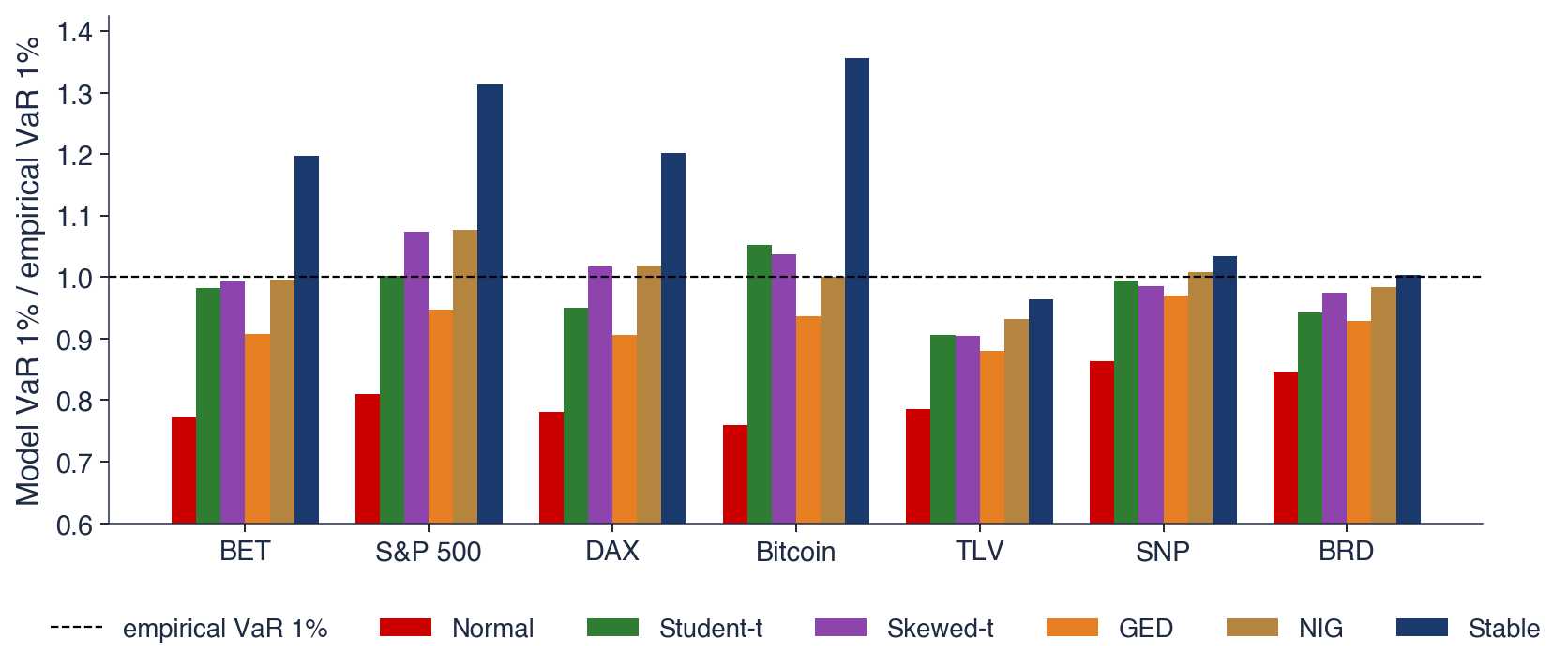
 SFM_ch6_candidates