Bucharest University of Economic Studies IDA Institute Digital Assets Blockchain Research Center AI4EFin Artificial Intelligence for Energy Finance Romanian Academy, Institute for Economic Forecasting MSCA Digital Finance
The question of the chapter is how the risks of several assets move together. In Chapter 5 the conditional variance of a single return series was enough to describe its risk. For a portfolio of two or more assets this is no longer enough: two portfolios with the same individual volatilities can have very different risk, depending on whether their components tend to fall on the same days or on different days. The quantity that captures this is the covariance, or its standardised version, the correlation, and the chapter treats both as variables that change from day to day.
The route goes from the general to the practical. It starts from the conditional covariance matrix \(\mathbf{H}_t\) and the two conditions it must satisfy, continues with the VEC and BEKK models, which describe all elements of \(\mathbf{H}_t\) at once, and arrives at the CCC and DCC models, which estimate volatilities and correlations separately. The last sections use these models for three applications: correlations in crises, the VaR of a portfolio and hedge ratios.
The chapter builds directly on three earlier ones. The univariate GARCH model of Chapter 5 is the building block of every multivariate model; the vector autoregression (VAR) of Chapter 6 supplies the multivariate notation and the idea of spillovers between series; cointegration, from Chapter 7, is the long-run counterpart of the short-run links studied here.
In brief
Question: how do the risks of several assets move together? Chapter 5 modelled the volatility of one series at a time
the risk of a portfolio, a hedge or the spread of a crisis depends on covariances and correlations, and these change in time
Route of the chapter
the conditional covariance matrix \(\mathbf{H}_t\) and its conditions
the VEC and BEKK models; the number of parameters
CCC and DCC: volatilities and correlations estimated in two steps
applications: correlations in crises, portfolio VaR 1%, hedge ratios
Self-study chapter
read the slides in order, redo the worked examples, run the notebook, then answer the self-assessment and the quiz
The first outcomes are conceptual. The reader should be able to explain why the variance of a portfolio, a hedge ratio and the question of contagion all depend on covariances that change over time, and to write the main multivariate GARCH models in matrix form. Counting the parameters of each model is part of understanding it: the count shows immediately which models can be estimated for five assets and which cannot.
The other outcomes are computational and empirical. One step of the DCC recursion can be computed by hand, and its parameters \(a\),\(b\) and \(a+b\) have a direct reading as the reaction to news, the persistence and the speed of return to the long-run correlation. A DCC model is estimated in two steps and compared with constant correlations by a likelihood ratio test. Finally, \(\mathbf{H}_t\) is turned into two practical numbers, the VaR 1% of a portfolio, judged by backtesting, and the minimum-variance hedge ratio, judged by its hedging effectiveness out of sample.
In brief
Explain why portfolio risk, hedging and contagion need a model for time-varying covariances
Write the VEC, BEKK, CCC and DCC models and count their parameters
Compute one step of the DCC recursion by hand and interpret \(a\), \(b\) and \(a+b\)
Estimate a DCC model in two steps and test it against constant correlations
Compute and backtest a portfolio VaR 1% from \(\mathbf{H}_t\)
Compute dynamic minimum-variance hedge ratios and their hedging effectiveness
The chapter's code uses the arch package for the univariate GARCH models of step 1. The package has no DCC model, so step 2 is written out in about 40 lines of numpy: the recursion for \(\mathbf{Q}_t\), the rescaling to correlations and the correlation part of the likelihood. Writing the recursion explicitly has a teaching advantage, since every element of the model is visible in the code. The lecture notebook reproduces the computations and the charts of the chapter.
Chapter 5 modelled the volatility of one return series at a time with generalised autoregressive conditional heteroskedasticity (GARCH) models. Most questions of risk management, however, concern several assets at once. The risk of a portfolio depends on how its components move together, a hedge works only as well as the link between the asset and the hedging instrument, and the spread of a crisis from one market to another is a statement about co-movement. All three questions are answered by covariances and correlations, and these change over time.
This chapter extends GARCH to \(N\) series. The object of interest is the conditional covariance matrix \(\mathbf{H}_t\), which holds the variances of all assets on its diagonal and their covariances off the diagonal. The chapter first sets out the conditions that any model for \(\mathbf{H}_t\) must respect, then presents the general VEC and BEKK models and the reason they become unusable beyond a few assets. The constant conditional correlation (CCC) and dynamic conditional correlation (DCC) models solve this by separating volatilities from correlations and estimating them in two steps.
The applications use daily data on the S&P 500, the German DAX index, the Romanian BET index, the EUR/RON exchange rate and Bitcoin. The correlation between the S&P 500 and the DAX is not constant: the likelihood ratio test against constant correlation gives 131.8, far above the 5% critical value of 5.99. Correlations rise in crises, most of all for the assets that are weakly linked to the large markets in calm times. The same conditional covariances give a portfolio Value at Risk (VaR) at 1% that adapts to the state of the market and dynamic hedge ratios that remove more risk out of sample than a static ratio.
The one-step-ahead DCC correlation of daily S&P 500 and DAX returns, the 250-day rolling correlation and the constant CCC value, 4 January 2000 – 18 September 2026.
What you will be able to do
Explain why portfolio risk, hedging and contagion need a model for time-varying covariances.
Write the VEC, BEKK, CCC and DCC models and count their parameters.
Compute one step of the DCC recursion by hand and interpret \(a\),\(b\) and \(a+b\).
Estimate a DCC model in two steps and test it against constant correlations.
Compute a portfolio VaR 1% from \(\mathbf{H}_t\) and backtest it with the Kupiec and Christoffersen tests.
Compute dynamic minimum-variance hedge ratios and their hedging effectiveness.
Chapter plan
Why multivariate volatilityPortfolio variance, hedging and contagion; rolling correlations and asynchronous trading.
SummaryKey ideas, formulas and self-assessment questions.
Why multivariate volatility
The section shows why a model for a single volatility is not enough. Portfolio risk, hedging and contagion all depend on correlations, and the correlations observed in real markets move a great deal over time. The section ends with a practical trap of daily data: markets that close at different hours.
The first question is the risk of a portfolio. If the vector \(\mathbf{w}\) holds the weights of the assets and \(\mathbf{H}\) is the covariance matrix of their returns, the variance of the portfolio return is a quadratic form, as in Markowitz (1952):
The first two terms come from the individual volatilities; the third is the only place where the joint behaviour enters. With positive weights, a lower correlation \(\rho\) means a lower portfolio variance, and this is the whole mechanism of diversification.
The second question is hedging: how many units of one asset to sell in order to offset the risk of another. Section 7 shows that the answer is the ratio of a covariance to a variance, so a hedge ratio moves whenever the covariance moves. The third question is contagion: do markets move more closely together in a crisis? Longin and Solnik (2001) found that correlations between international equity markets are higher in bear markets. If correlations rise exactly when volatility rises, diversification weakens at the moment it is needed most.
A univariate GARCH model gives the volatilities \(\sigma_{1,t}\) and \(\sigma_{2,t}\) day by day. Formula (14.1) also needs the correlation, and the aim of this chapter is to add a correlation \(\rho_t\) that changes over time in the same way.
In brief
Portfolio risk
the variance of a portfolio with weights \(\mathbf{w}\) is \(\sigma_p^2 = \mathbf{w}^\top\mathbf{H}\mathbf{w}\)Markowitz (1952)
\(\mathbf{w}\): the vector of portfolio weights; \(\mathbf{H}\): the covariance matrix of the returns; \(\sigma_p^2\): the portfolio variance
two assets: \(\sigma_p^2 = w_1^2\sigma_1^2 + w_2^2\sigma_2^2 + 2w_1w_2\rho\,\sigma_1\sigma_2\), with volatilities \(\sigma_1\), \(\sigma_2\) and correlation \(\rho\)
the correlation \(\rho\) decides how much diversification helps
Hedging
how many units of an asset to sell to offset the risk of another
the answer is a ratio of a covariance to a variance (Section 7)
Contagion
do markets move more closely together in a crisis?
if correlations rise exactly when volatility rises, diversification fails when it is needed most Longin and Solnik (2001)
A univariate GARCH (Chapter 5) gives \(\sigma_{1,t}\) and \(\sigma_{2,t}\); this chapter adds the time-varying \(\rho_t\)
Take two assets with an annual volatility of 20% each and a portfolio split 50/50. With volatilities in percent, \(\sigma_1^2 = \sigma_2^2 = 400\) and \(w_1^2 = w_2^2 = 0.25\), so the first two terms of (14.1) add up to 200 whatever the correlation. With \(\rho = 0.2\) the covariance term is \(2 \cdot 0.25 \cdot 0.2 \cdot 400 = 40\), the variance is 240 and the volatility \(\sqrt{240} = 15.5\%\). With \(\rho = 0.8\) the covariance term is 160, the variance 360 and the volatility 19.0%.
Nothing changed except the correlation: the same assets, the same weights, the same individual volatilities. Yet the risk of the portfolio rises by more than a fifth. The practical consequence is that a risk model which keeps \(\rho\) at the value it had in a calm period understates the risk when correlations rise, and the data below show that they do rise in crises.
In brief
Two assets with annual volatility 20% each, weights 50% and 50%
Question for the room ▶ raises ρ from 0.3 to 1 in steps of 0.1. Does σp rise by the same amount at every step?
Answer
No: +0.63 points from ρ = 0.2 to 0.3 (from 15.49% to 16.12%), but only +0.51 points from 0.9 to 1 (from 19.49% to 20%). σp2 is linear in ρ and σp is its square root, so the curve is concave. With ρ = −0.2 the volatility is 12.6%.
Question for the room ▶ moves the weight of the first asset from 60% to 90% (both assets at 20%). What happens to σp for ρ = 0.8?
Answer
It rises: 19.02% at 60% and 19.64% at 90%, against 18.97% at 50/50. With equal volatilities the 50/50 portfolio has the lowest risk whatever ρ. With the second asset at 40% and ρ = −1, σp = |0.5 · 20 − 0.5 · 40| = 10%: the risk disappears only with w = 2/3.
The chart plots the annual volatility of the 50/50 portfolio, in percent, on the vertical axis against the correlation \(\rho\) on the horizontal axis, from \(-1\) to \(1\), with both assets at 20% volatility. The two marked points are the cases of the worked example: 15.5% at \(\rho = 0.2\) and 19.0% at \(\rho = 0.8\).
The curve is the square root of a linear function of \(\rho\): for this portfolio \(\sigma_p^2 = 200 + 200\rho\). It starts at zero for \(\rho = -1\), rises steeply at first and then more slowly, and reaches 20% at \(\rho = 1\). Reading the chart from right to left gives the benefit of diversification, the vertical distance between the curve and the 20% level at each correlation.
In brief
A 50/50 portfolio of two assets with 20% volatility each; the points are the two cases of the worked example
Three points of the curve are worth remembering. At \(\rho = 1\) the two assets move as one, there is no diversification and the portfolio has the 20% volatility of each asset. At \(\rho = 0\) the covariance term disappears and the volatility is \(20/\sqrt{2} \approx 14.1\%\). At \(\rho = -1\) the movements of the two assets cancel exactly and the risk disappears, a case that does not occur with real equity indices.
Because the curve is concave, the same increase of the correlation adds more volatility at low correlations than at high ones. For portfolios that combine weakly correlated assets, the very portfolios built for diversification, a rise in correlation is therefore most costly. This leads to the empirical question of the chapter: does \(\rho\) stay put in real markets, or does it move with the state of the market?
Question for the room ▶ sums the daily returns over k = 2, …, 10 days. What happens to the S&P 500 – BET correlation?
Answer
It rises: 0.32 daily, 0.40 over 2 days and 0.50 over 10 days, above the weekly correlation of 0.46: news that reaches Bucharest a day later falls into the same k-day return. Of the ten pairs, only the S&P 500 and Bitcoin have a weekly correlation below the daily one (0.25 → 0.19): the weekly Bitcoin return also contains the weekend, and the 610 weeks give a noisier estimate than the 2,815 days.
Question for the room ▶ lengthens the window up to 500 days. What happens to the minimum of the S&P 500 – DAX correlation (0.21 at 250 days)?
Answer
It rises to 0.30 (November 2025): in a long window the asynchronous days of April 2025 weigh less. With 60 days the correlation goes down to −0.27 (July 2025) and up to 0.86 (January 2012), with a standard deviation of 0.147 against 0.122 at 250 days.
A first answer comes from rolling correlations (rolling windows): the sample correlation of daily log returns computed over the last 250 trading days, about one year, and dated at the end of the window. The chart plots this correlation on the vertical axis against time on the horizontal axis for three pairs: the S&P 500 and the DAX, from 2001; the BET and the DAX, from 2001; the S&P 500 and Bitcoin, from 2015. The shaded bands mark September 2008 – March 2009 and February – April 2020, and a dashed line marks zero.
Each correlation uses only the days on which both markets trade, so that each pair of returns refers to the same calendar day. A rolling correlation is a descriptive tool, not a model: it gives every day in the window the same weight and forgets everything older than 250 days. It is useful here because it shows, without any assumption about dynamics, whether the correlation is stable.
In brief
Correlation of daily log returns over rolling windows of 250 trading days (about one year), dated at the window end
returns on the days on which both markets trade; shaded: September 2008–March 2009 and February–April 2020
None of the three correlations is stable. The S&P 500 and the DAX range between 0.21 in April 2026 and 0.80 in October 2012, around a full-sample value of 0.60. The highest values do not come in 2008 but during the euro-area debt crisis of 2010–2012, which tied the two markets even more closely.
The BET and the DAX show a slower change. Before 2007 the correlation was close to zero, with a minimum of \(-0.08\); after Romania joined the European Union (EU) it rose in steps, up to 0.70 in August 2020. The Romanian market became integrated with European markets, and its value for diversifying a European portfolio fell accordingly. The S&P 500 and Bitcoin went from \(-0.16\) in December 2019 to 0.57 in February 2023: after 2020 Bitcoin behaved more like a risk asset correlated with equities.
The conclusion is that correlations wander far from any constant value, over years through integration and within months through crises. A model must let them move.
In brief
S&P 500 and DAX: between 0.21 (April 2026) and 0.80 (October 2012); full-sample value 0.60
the euro-area debt crisis of 2010–2012 tied the two markets even more closely than 2008
BET and DAX: close to zero before 2007 (minimum \(-\)0.08), up to 0.70 in August 2020: the Romanian market became integrated with Europe after EU accession
S&P 500 and Bitcoin: from \(-\)0.16 (December 2019) to 0.57 (February 2023); Bitcoin became a risk asset correlated with equities after 2020
Correlations wander far from any constant value: a model must let them move
Asynchronous trading and the bias of daily correlations
Daily returns of different markets do not cover the same hours. Bucharest closes at 16:45 Central European Time (CET), 17:45 local time, Frankfurt at 17:30 CET and New York at 22:00 CET, while Bitcoin trades all day, every day. News that arrives after the European close enters European prices only on the next trading day. This is asynchronous trading (non-synchronous trading), and it splits the reaction to one event across two daily returns.
The tariff announcement of 9 April 2025 shows the effect. The pause of the United States (US) tariffs was announced in the afternoon in New York, after the European close: on 9 April the S&P 500 rose by 9.1% and the DAX fell by 3.1%; on 10 April the S&P 500 fell by 3.5% and the DAX rose by 4.4%. The same news produced returns of opposite sign on the same calendar day, and this pulls the daily correlation towards zero.
Weekly returns are much less affected, because a one-day delay matters little over five days. Since 2015 the correlation of daily against weekly returns is 0.32 against 0.46 for the S&P 500 and the BET, 0.56 against 0.68 for the S&P 500 and the DAX, and 0.42 against 0.47 for the BET and the DAX. The gap is small for the last pair, whose markets close almost together. The remedies are weekly returns or returns measured between synchronous times; the daily models of this chapter keep the bias in mind when reading transatlantic correlations.
In brief
Markets close at different hours: Bucharest at 16:45 CET (17:45 local time), Frankfurt at 17:30 CET, New York at 22:00 CET; Bitcoin trades all day, every day
news that arrives after the European close shows up in the European prices only the next day
Example: 9 April 2025, the pause of the US tariffs announced in the afternoon in New York
the same news, on two different days: the daily correlation is biased towards zero
Correlations of daily and weekly returns since 2015: S&P 500 and BET 0.32 against 0.46; S&P 500 and DAX 0.56 against 0.68; BET and DAX 0.42 against 0.47
the gap is small for BET and DAX, which close almost together; remedies: weekly returns or returns between synchronous times
The portfolio variance \(\mathbf{w}^\top\mathbf{H}\mathbf{w}\), the hedge ratio and the question of contagion all depend on covariances. Rolling correlations of real markets move a great deal, through market integration, through crises and through the arrival of new asset classes such as Bitcoin. Before computing any daily correlation, the trading hours must be checked, because asynchronous closes bias daily correlations towards zero.
In brief
Portfolio variance \(\mathbf{w}^\top\mathbf{H}\mathbf{w}\), hedge ratios and contagion all depend on covariances
Rolling correlations of real markets move a lot: integration, crises, new asset classes
Check the trading hours: asynchronous closes bias daily correlations towards zero
Section summary
The section has motivated a model in which correlations change over time; rolling windows show the change but do not explain it and depend on an arbitrary window length. The next section sets up the general framework, a conditional covariance matrix that is updated every day from past shocks, and the conditions it must satisfy.
The multivariate GARCH framework
The section defines the multivariate GARCH model in general form: the vector of returns, the conditional covariance matrix \(\mathbf{H}_t\), the conditions of symmetry and positive definiteness, and estimation by maximum likelihood.
Here \(\mathbf{r}_t\) is the vector of the \(N\) returns on day \(t\),\(\boldsymbol{\mu}\) the vector of means (or the forecast of a VAR model, as in Chapter 6), and \(\boldsymbol{\eta}_t\) a vector of independent and identically distributed (i.i.d.) innovations with mean zero and covariance matrix \(\mathbf{I}_N\). The matrix \(\mathbf{H}_t^{1/2}\) is a square root of \(\mathbf{H}_t\), for instance the Cholesky factor \(\mathbf{L}_t\) with \(\mathbf{L}_t\mathbf{L}_t^\top = \mathbf{H}_t\); any such root gives the shocks \(\boldsymbol{\varepsilon}_t\) the conditional covariance matrix \(\mathbf{H}_t\).
The conditional covariance matrix (conditional covariance matrix) \(\mathbf{H}_t\) is computed from the information \(\mathcal{F}_{t-1}\) available up to day \(t-1\). Its diagonal holds the conditional variances \(h_{ii,t} = \sigma_{i,t}^2\), exactly the quantities of Chapter 5. Off the diagonal are the conditional covariances \(h_{ij,t}\), and the conditional correlation follows from them:
A multivariate GARCH (MGARCH) model is a rule that computes \(\mathbf{H}_t\) from the past shocks \(\boldsymbol{\varepsilon}_{t-1}\) and from \(\mathbf{H}_{t-1}\). The models of the following sections differ only in this rule.
In brief
\(\mathbf{r}_t = \boldsymbol{\mu} + \boldsymbol{\varepsilon}_t\), \(\boldsymbol{\varepsilon}_t = \mathbf{H}_t^{1/2}\boldsymbol{\eta}_t\), \(\boldsymbol{\eta}_t\) i.i.d. with mean \(\mathbf{0}\) and covariance \(\mathbf{I}_N\)
\(\mathbf{r}_t\): the vector of \(N\) returns on day \(t\); \(\boldsymbol{\mu}\): the means (or a VAR model for the mean, Chapter 6)
\(\mathbf{H}_t^{1/2}\): a square root of \(\mathbf{H}_t\), e.g. the Cholesky factor \(\mathbf{L}_t\) with \(\mathbf{L}_t\mathbf{L}_t^\top = \mathbf{H}_t\)
\(\mathbf{H}_t = \Var(\mathbf{r}_t \mid \mathcal{F}_{t-1})\): the conditional covariance matrix, given the information \(\mathcal{F}_{t-1}\) up to day \(t-1\)
diagonal: the conditional variances \(h_{ii,t} = \sigma_{i,t}^2\) (Chapter 5)
off-diagonal: the conditional covariances \(h_{ij,t}\); the conditional correlation is \(\rho_{ij,t} = h_{ij,t}/\sqrt{h_{ii,t}h_{jj,t}}\)
A multivariate GARCH (MGARCH) model is a rule that computes \(\mathbf{H}_t\) from past shocks \(\boldsymbol{\varepsilon}_{t-1}\) and past \(\mathbf{H}_{t-1}\)
The first condition is symmetry: the covariance of asset \(i\) with asset \(j\) is the covariance of \(j\) with \(i\), so \(h_{ij,t} = h_{ji,t}\) and only the \(N(N+1)/2\) elements on and below the diagonal are distinct. The operator \(\mathrm{vech}\) stacks these elements column by column in a vector; for two assets, \(\mathrm{vech}(\mathbf{H}) = (h_{11}, h_{12}, h_{22})^\top\). The number of distinct elements grows quickly: 3 for \(N = 2\), 55 for \(N = 10\) and 1 275 for \(N = 50\).
The second condition is positive definiteness (positive definiteness): \(\mathbf{w}^\top\mathbf{H}_t\mathbf{w} > 0\) for every non-zero vector \(\mathbf{w}\). By (14.1) the left side is the variance of the portfolio with weights \(\mathbf{w}\), so the condition says that every portfolio has a positive variance. For two assets it reduces to \(h_{11,t} > 0\) and \(h_{11,t}h_{22,t} - h_{12,t}^2 > 0\), which is the same as \(|\rho_{12,t}| < 1\).
The example on the slide shows what goes wrong without this condition. With \(h_{11} = 4\),\(h_{22} = 1\) and \(h_{12} = 2.5\) the determinant is \(4 - 6.25 < 0\), and (14.3) gives a "correlation" of 1.25, which no pair of random variables can have. A model that computes each element of \(\mathbf{H}_t\) separately can produce such matrices. A good MGARCH model guarantees both conditions for every \(t\), whatever the shocks, and does so with few parameters.
In brief
Symmetry
\(h_{ij,t} = h_{ji,t}\), so only \(N(N+1)/2\) elements are distinct
the operator \(\mathrm{vech}\) stacks the lower triangle: \(\mathrm{vech}\begin{pmatrix} h_{11} & h_{12}\\ h_{12} & h_{22}\end{pmatrix} = (h_{11}, h_{12}, h_{22})^\top\)
If the innovations \(\boldsymbol{\eta}_t\) follow the multivariate Normal distribution, the shocks \(\boldsymbol{\varepsilon}_t\) are conditionally Normal with covariance matrix \(\mathbf{H}_t\), and the log-likelihood of the sample is
where \(|\mathbf{H}_t|\) is the determinant and \(\theta\) collects all parameters. For \(N = 1\) the determinant is \(\sigma_t^2\), the quadratic form is \(\varepsilon_t^2/\sigma_t^2\), and (14.4) becomes the GARCH likelihood of Chapter 5. The two terms play the same roles as there: the determinant penalises large variances, the quadratic form penalises shocks that are large relative to the predicted covariance.
Daily returns have fat tails, so the Normal assumption is not literally true. The Normal likelihood is then used as a quasi-maximum likelihood (QML): the estimates of the parameters of \(\mathbf{H}_t\) remain consistent as long as \(\mathbf{H}_t\) is correctly specified, but the usual standard errors are wrong and need a robust (sandwich) correction.
The practical difficulty is computational. Each evaluation of \(\ell(\theta)\) requires the inverse and the determinant of \(\mathbf{H}_t\) for every day of the sample, and a numerical optimiser evaluates \(\ell(\theta)\) many times. The cost grows quickly with \(N\) and, above all, with the number of parameters, which is the subject of the next section.
In brief
If \(\boldsymbol{\eta}_t\) follows the multivariate Normal distribution, the log-likelihood is
\(|\mathbf{H}_t|\) is the determinant; for \(N = 1\) this is the GARCH likelihood of Chapter 5
Returns have fat tails, so the Normal likelihood is used as quasi-maximum likelihood (QML)
the estimates stay consistent; the standard errors need a robust (sandwich) correction
Every evaluation of \(\ell(\theta)\) needs \(\mathbf{H}_t^{-1}\) and \(|\mathbf{H}_t|\) for all \(t\): the cost grows fast with \(N\) and with the number of parameters
The conditional covariance matrix \(\mathbf{H}_t\) has the conditional variances on its diagonal and the covariances off it, and the conditional correlation follows from (14.3). A valid model must keep \(\mathbf{H}_t\) symmetric, with \(N(N+1)/2\) distinct elements, and positive definite on every day. Estimation uses the multivariate Normal likelihood (14.4), as a quasi-likelihood when returns have fat tails.
In brief
\(\mathbf{H}_t\): conditional variances on the diagonal, covariances off the diagonal; \(\rho_{ij,t} = h_{ij,t}/\sqrt{h_{ii,t}h_{jj,t}}\)
Conditions: symmetry (\(N(N+1)/2\) distinct elements) and positive definiteness
Estimation by (quasi-)maximum likelihood with the multivariate Normal density
Section summary
The framework leaves open the rule that updates \(\mathbf{H}_t\). The next section presents the two classic answers, VEC and BEKK, which model all elements of the matrix at once, and shows the price they pay in parameters.
VEC and BEKK models
The section presents the most general linear MGARCH model, VEC, and the BEKK model, which guarantees positive definiteness by construction. Counting their parameters shows why neither can be used for more than a handful of assets.
Bollerslev, Engle and Wooldridge (1988) wrote the most general linear extension of GARCH(1,1): every distinct element of \(\mathbf{H}_t\) depends on every past squared shock and cross-product and on every element of \(\mathbf{H}_{t-1}\). With the \(\mathrm{vech}\) operator, the VEC(1,1) model is
The matrix \(\boldsymbol{\varepsilon}_{t-1}\boldsymbol{\varepsilon}_{t-1}^\top\) holds yesterday's squared shocks on its diagonal and their cross-products off it. The vector \(\mathbf{c}\) holds constants, \(\mathbf{A}\) measures the reaction to shocks and \(\mathbf{B}\) the persistence, as \(\omega\),\(\alpha\) and \(\beta\) do in a univariate GARCH.
The generality is expensive. With \(k = N(N+1)/2\) distinct elements, \(\mathbf{c}\) has \(k\) entries and \(\mathbf{A}\) and \(\mathbf{B}\) are \(k \times k\), so the model has \(k + 2k^2\) parameters: 21 for two assets and 6 105 for ten. Worse, nothing in (14.5) keeps \(\mathbf{H}_t\) positive definite; the restrictions that would do so are complicated and hard to impose during estimation.
The diagonal VEC keeps only the diagonal of \(\mathbf{A}\) and \(\mathbf{B}\), so that each element follows its own GARCH(1,1):
This leaves \(3k\) parameters, 9 for \(N = 2\), but positive definiteness is still not guaranteed, because each element is updated without regard to the others.
In brief
Bollerslev, Engle and Wooldridge (1988): every element of \(\mathbf{H}_t\) depends on every past squared shock, cross-product and element of \(\mathbf{H}_{t-1}\)
\(\boldsymbol{\varepsilon}_{t-1}\boldsymbol{\varepsilon}_{t-1}^\top\): the matrix of yesterday's squared shocks and cross-products; \(\mathbf{c}\): a vector of constants; \(\mathbf{A}\): the reaction to shocks; \(\mathbf{B}\): the persistence
with \(k = N(N+1)/2\): \(\mathbf{c}\) has \(k\) elements, \(\mathbf{A}\) and \(\mathbf{B}\) are \(k \times k\): in total \(k + 2k^2\) parameters
with \(\mathbf{C}\) lower triangular and \(\mathbf{A}\),\(\mathbf{B}\) full \(N \times N\) matrices. \(\mathbf{A}\) describes the reaction to yesterday's shocks and \(\mathbf{B}\) the persistence of \(\mathbf{H}_{t-1}\); the elements of the constant matrix \(\mathbf{C}\mathbf{C}^\top\) are written \(c_{ij}^*\).
The guarantee comes from the form of each term, a "square" \(\mathbf{X}^\top\mathbf{M}\mathbf{X}\) of a positive semidefinite matrix \(\mathbf{M}\): the identity in the first term (with \(\mathbf{X} = \mathbf{C}^\top\)), the outer product \(\boldsymbol{\varepsilon}_{t-1}\boldsymbol{\varepsilon}_{t-1}^\top\) in the second and \(\mathbf{H}_{t-1}\) in the third. For any vector \(\mathbf{w}\),
and a constant term \(\mathbf{C}\mathbf{C}^\top\) of full rank makes the sum strictly positive. The number of parameters is \(N(N+1)/2 + 2N^2\): 11 for two assets, 255 for ten.
The off-diagonal elements of a full \(\mathbf{A}\) have an economic meaning: they measure volatility spillovers (volatility spillovers), the effect of a shock to asset 1 on the variance of asset 2. Restricting \(\mathbf{A}\) and \(\mathbf{B}\) to be diagonal gives the diagonal BEKK, in which the covariance follows
The scalar BEKK goes further, with \(\mathbf{A} = a\mathbf{I}\) and \(\mathbf{B} = b\mathbf{I}\), so that all elements share the same dynamics. Both restrictions save parameters and remove the spillovers.
BEKK: Baba, Engle, Kraft and Kroner; \(\mathbf{C}\) lower triangular, \(\mathbf{A}\) and \(\mathbf{B}\) are \(N \times N\)
\(\mathbf{A}\): the reaction to yesterday's shocks; \(\mathbf{B}\): the persistence of \(\mathbf{H}_{t-1}\); \(c_{ij}^*\): the elements of \(\mathbf{C}\mathbf{C}^\top\)
Positive definite by construction
each term is a “square” \(\mathbf{X}^\top\mathbf{M}\mathbf{X}\) of a positive (semi)definite matrix \(\mathbf{M}\)
\(\mathbf{M}\): \(\mathbf{I}\), \(\boldsymbol{\varepsilon}_{t-1}\boldsymbol{\varepsilon}_{t-1}^\top\) or \(\mathbf{H}_{t-1}\); \(\mathbf{X}\): \(\mathbf{C}^\top\), \(\mathbf{A}\) or \(\mathbf{B}\)
parameters: \(N(N+1)/2 + 2N^2\), i.e. 11 for \(N = 2\) and 255 for \(N = 10\)
The covariance equation of a diagonal BEKK can be computed by hand. The given values are \(c_{12}^* = 0.02\),\(a_{11} = 0.30\),\(a_{22} = 0.25\),\(b_{11} = 0.94\),\(b_{22} = 0.95\), yesterday's covariance \(h_{12,t-1} = 0.5\) and yesterday's shocks \(\varepsilon_{1,t-1} = -2\) and \(\varepsilon_{2,t-1} = -1.5\). The coefficients of the covariance equation are products: \(a_{11}a_{22} = 0.075\) for the reaction to the cross-product of shocks and \(b_{11}b_{22} = 0.893\) for persistence.
The cross-product of the shocks is \((-2)(-1.5) = 3.000\), positive because both assets fell. Today's covariance is
A joint fall raises the covariance from 0.5 to 0.6915; a shock with opposite signs would have given a negative cross-product and lowered it.
The example also shows what the diagonal model cannot do. Because \(a_{12} = a_{21} = 0\), a shock to asset 1 affects the variance of asset 2 only through the covariance, never directly: the diagonal BEKK has no volatility spillovers.
The table counts the parameters of the variance equation of each model for 2, 5, 10 and 50 assets; the means \(\boldsymbol{\mu}\) are not counted. For CCC and DCC, introduced in the next section, the count is 3 GARCH parameters per asset plus the \(N(N-1)/2\) correlations, and DCC adds 2 more.
The rows differ by orders of magnitude. The full VEC needs 21 parameters for two assets, 465 for five, 6 105 for ten and 3 252 525 for fifty: for fifty assets it has more parameters than any sample of daily data has observations. The full BEKK is much more economical but still reaches 6 275 parameters for fifty assets. The diagonal BEKK, CCC and DCC stay close to each other, with 1 375 to 1 377 parameters for fifty assets, and the scalar BEKK is the cheapest, with 1 277. This growth of the number of parameters with the dimension is called the curse of dimensionality (curse of dimensionality).
In brief
Model
\(N = 2\)
\(N = 5\)
\(N = 10\)
\(N = 50\)
VEC(1,1)
21
465
6 105
3 252 525
Diagonal VEC
9
45
165
3 825
BEKK(1,1)
11
65
255
6 275
Diagonal BEKK
7
25
75
1 375
Scalar BEKK
5
17
57
1 277
CCC
7
25
75
1 375
DCC
9
27
77
1 377
Number of parameters of the variance equation (the means \(\boldsymbol{\mu}\) are not counted); CCC and DCC: 3 GARCH parameters per asset plus the \(N(N-1)/2\) correlations, and 2 more for DCC
A full VEC for 50 assets has more parameters than any sample has observations
Question for the room ▶ lowers h12 from 2.75 to −3 (h11 = 4, h22 = 1). For which values is H positive definite?
Answer
Only for |h12| < 2, i.e. |ρ| < 1. At h12 = ±2 the determinant and one eigenvalue are 0 (a riskless combination); for |h12| > 2 some portfolios have a negative variance, for example −0.416 for h12 = ±2.5. The sign of the covariance does not matter, only its size against √(h11h22).
Question for the room Set ε2,t−1 = +1.5 (the opposite sign of ε1,t−1 = −2). What is h12,t?
Answer
0.2415 = 0.020 + 0.075 · (−3) + 0.4465: shocks of opposite signs lower the covariance. With ε2,t−1 = 0, h12,t = 0.4665, still below 0.5, although the long-run level is 0.625: that level accounts for the cross-product of the shocks being equal to h12 on average, and a day without a joint shock brings only the constant and the persistence.
Question for the room For N = 30, BEKK(1,1) has 2,265 parameters. How many does DCC have?
Answer
527: 90 GARCH parameters estimated series by series, 435 sample correlations and only 2 parameters, a and b, found by numerical optimisation. VEC(1,1) has 432,915.
Question for the room ▶ raises the largest N up to 100. By what factor does the number of VEC(1,1) parameters grow from N = 50 to N = 100?
Answer
15.7 times (from 3,252,525 to 51,010,050), like N4: 24 = 16. DCC grows 3.8 times (from 1,377 to 5,252), BEKK(1,1) 4 times (from 6,275 to 25,050).
The chart plots the number of parameters of the variance equation, on a logarithmic vertical axis, against the number of assets \(N\), from 2 to 50, for six models: VEC(1,1), BEKK(1,1), diagonal VEC, diagonal BEKK, DCC and CCC. The scalar BEKK, from the table, is not drawn.
On a logarithmic scale a constant vertical distance means a constant ratio. The VEC curve lies far above all others and keeps moving away, passing \(10^6\) at \(N = 50\). The full BEKK and the diagonal VEC lie in between, and the last three curves (diagonal BEKK, DCC and CCC) almost coincide, because their counts differ by at most two parameters.
In brief
Number of parameters of the variance equation for \(N = 2, \dots, 50\) assets, log scale
The leading terms of the formulas give the growth rates. For VEC, \(2k^2\) with \(k \approx N^2/2\) grows like \(N^4/2\); for the full BEKK the count grows like \(2N^2\). Both become impossible to estimate beyond a handful of assets, because a numerical optimiser cannot search reliably over hundreds or thousands of parameters with a likelihood like (14.4).
CCC and DCC grow like \(N^2/2\), but the count hides an important difference: the correlations are not found by numerical optimisation. As the next section shows, they are sample correlations of standardised residuals, computed directly. The GARCH parameters are estimated one series at a time, with three parameters each. The only joint optimisation in DCC concerns two parameters, \(a\) and \(b\), whatever the number of assets. This is why DCC can be used where VEC and BEKK cannot.
In brief
VEC grows like \(N^4/2\), full BEKK like \(2N^2\): both become impossible to estimate beyond a handful of assets
CCC and DCC grow like \(N^2/2\), but the correlations are not found by numerical optimisation: they are sample correlations (Section 4)
the DCC optimiser works on only 2 parameters, \(a\) and \(b\), whatever \(N\)
VEC is the most general linear model, with \(k + 2k^2\) parameters and no guarantee of positive definiteness. BEKK is positive definite by construction, and the off-diagonal elements \(a_{ij}\) of its matrix \(\mathbf{A}\) measure volatility spillovers. The diagonal and scalar versions cut the number of parameters but remove the spillovers.
In brief
VEC: the most general linear model; \(k + 2k^2\) parameters, no positive-definiteness guarantee
BEKK: positive definite by construction; off-diagonal \(a_{ij}\) measure volatility spillovers
Diagonal and scalar versions cut the parameters but remove the spillovers
Section summary
VEC and BEKK model the whole matrix \(\mathbf{H}_t\) in one equation, and this is the source of their cost. The next section takes a different route: it splits \(\mathbf{H}_t\) into volatilities, which univariate GARCH models already handle, and a correlation matrix with very few dynamic parameters.
Constant and dynamic conditional correlations
The section decomposes the covariance matrix into volatilities and correlations, presents the constant conditional correlation model and Engle's dynamic conditional correlation model, explains their estimation in two steps and the test of DCC against CCC.
where \(\mathbf{R}_t\) is the conditional correlation matrix, with ones on the diagonal. Element by element, \(h_{ij,t} = \rho_{ij,t}\,\sigma_{i,t}\sigma_{j,t}\), which is (14.3) read the other way. Each volatility follows a univariate GARCH(1,1) model (Bollerslev, 1986):
Dividing each shock by its own volatility gives the standardised residuals (standardised residuals) \(z_{i,t} = \varepsilon_{i,t}/\sigma_{i,t}\). Each has conditional variance one, and the conditional covariance of \(z_{i,t}\) and \(z_{j,t}\) is \(h_{ij,t}/(\sigma_{i,t}\sigma_{j,t}) = \rho_{ij,t}\). The conditional covariance matrix of the vector \(\mathbf{z}_t\) is therefore exactly \(\mathbf{R}_t\): once the volatilities are removed, only the correlations are left to model.
The simplest choice is the constant conditional correlation (CCC) model of Bollerslev (1990), with \(\mathbf{R}_t = \mathbf{R}\) for all \(t\).\(\mathbf{H}_t\) is then positive definite whenever \(\mathbf{R}\) is and the GARCH variances are positive, and \(\mathbf{R}\) is estimated by the sample correlation matrix of the \(z_{i,t}\). In CCC the covariances still move, but only through the volatilities. The rolling correlations of the first section contradict this assumption.
\(\mathbf{R}_t\): the conditional correlation matrix (ones on the diagonal); element by element: \(h_{ij,t} = \rho_{ij,t}\,\sigma_{i,t}\sigma_{j,t}\)
each \(\sigma_{i,t}\) is a univariate GARCH(1,1) Bollerslev (1986): \(\sigma_{i,t}^2 = \omega_i + \alpha_i\varepsilon_{i,t-1}^2 + \beta_i\sigma_{i,t-1}^2\)
Standardised residuals
\(z_{i,t} = \varepsilon_{i,t}/\sigma_{i,t}\)
their conditional covariance matrix is exactly \(\mathbf{R}_t\)
Robert F. Engle, born in 1942, received the Nobel Prize in economics in 2003 for methods of analysing economic time series with time-varying volatility. Engle (2002) proposed letting the correlations follow a recursion of the same form as GARCH. An auxiliary matrix \(\mathbf{Q}_t\), with elements \(q_{ij,t}\), is updated each day from yesterday's vector of standardised residuals:
The rescaling in the second part is needed because \(\mathbf{Q}_t\) is a weighted average of matrices whose diagonals are not exactly one; dividing by the square roots of the diagonal turns it into a proper correlation matrix with ones on the diagonal.
\(\bar{\mathbf{Q}}\) is the unconditional correlation matrix of \(\mathbf{z}_t\), and it is set to its sample value before the optimisation. This is correlation targeting (correlation targeting): the recursion is anchored at the observed long-run correlation, and only \(a\) and \(b\) remain to be estimated. The parameter \(a \ge 0\) is the reaction to yesterday's joint shock, \(b \ge 0\) the persistence, and \(a + b < 1\) ensures that \(\mathbf{Q}_t\) reverts to \(\bar{\mathbf{Q}}\).
With \(a = b = 0\) the recursion gives \(\mathbf{Q}_t = \bar{\mathbf{Q}}\) on every day, which is CCC. DCC therefore contains CCC as a special case, and this nesting is what makes a likelihood ratio test between the two possible.
Substituting (14.7) into the log-likelihood (14.4) splits it into two parts, \(\ell = \ell_V(\theta_1) + \ell_C(\theta_1, a, b)\). The volatility part \(\ell_V\) depends only on \(\theta_1\), the GARCH parameters of all series, and is the sum of the univariate GARCH likelihoods. The correlation part \(\ell_C\) depends on \(\theta_1\) through the standardised residuals and on \(a\) and \(b\).
The split suggests estimating in two steps. In step 1 a GARCH(1,1) is fitted to each series separately, as in Chapter 5, and the fitted volatilities \(\hat\sigma_{i,t}\) and standardised residuals \(\hat z_{i,t} = \hat\varepsilon_{i,t}/\hat\sigma_{i,t}\) are kept. In step 2, \(\bar{\mathbf{Q}}\) is set to the sample correlation of \(\hat{\mathbf{z}}_t\) and the correlation log-likelihood is maximised over \((a, b)\) only:
\[\ell_C(a, b) = -\frac12\sum_{t=1}^{T}\left(\log|\mathbf{R}_t| + \hat{\mathbf{z}}_t^\top\mathbf{R}_t^{-1}\hat{\mathbf{z}}_t - \hat{\mathbf{z}}_t^\top\hat{\mathbf{z}}_t\right).\]
(14.9)
The estimator is consistent, fast and works for large \(N\). Its weak point is inference: the standard errors of step 2 treat the step-1 estimates as known and ignore their estimation error, so they are too small.
The test against CCC compares the maximised correlation log-likelihoods: \(LR = 2(\ell_C^{DCC} - \ell_C^{CCC})\), compared with the \(\chi^2(2)\) distribution, whose 5% critical value is 5.99. A large value rejects constant correlation. Because the null hypothesis \(a = b = 0\) lies on the boundary of the parameter space, the \(\chi^2(2)\) critical value is conservative: a rejection with it is a safe rejection. Tse (2000) proposed another test of constant correlations, based on the Lagrange multiplier principle.
In brief
The log-likelihood splits into a volatility part and a correlation part: \(\ell = \ell_V(\theta_1) + \ell_C(\theta_1, a, b)\)
\(\theta_1\): the GARCH parameters of all series; \(\ell_V\) depends only on them, \(\ell_C\) also on \(a\) and \(b\)
Step 1
fit a GARCH(1,1) to each series separately (Chapter 5)
keep \(\hat\sigma_{i,t}\) and \(\hat z_{i,t} = \hat\varepsilon_{i,t}/\hat\sigma_{i,t}\)
Step 2
set \(\bar{\mathbf{Q}}\) to the sample correlation of \(\hat{\mathbf{z}}_t\) and maximise over \((a, b)\) only
\(\ell_C(a, b) = -\frac12\sum_t\left(\log|\mathbf{R}_t| + \hat{\mathbf{z}}_t^\top\mathbf{R}_t^{-1}\hat{\mathbf{z}}_t - \hat{\mathbf{z}}_t^\top\hat{\mathbf{z}}_t\right)\)
Consistent, fast, works for large \(N\); the step-2 standard errors ignore the estimation error of step 1 (they are too small)
Test against CCC
likelihood ratio \(LR = 2(\ell_C^{DCC} - \ell_C^{CCC})\), compared with \(\chi^2(2)\) (5% critical value 5.99)
The recursion (14.8) can be followed by hand for two assets. The given values are \(a = 0.05\),\(b = 0.93\), a long-run correlation \(\bar q_{12} = 0.5\) (with \(\bar q_{11} = \bar q_{22} = 1\)), yesterday's matrix \(\mathbf{Q}_{t-1}\) with ones on the diagonal and 0.5 off it, and yesterday's standardised residuals \(z_{1,t-1} = -2\) and \(z_{2,t-1} = -2.5\), a large joint fall. The weight of the long-run matrix is \(1 - a - b = 0.020\).
The off-diagonal element and, because the squared residuals enter them, the diagonal elements are
The correlation is \(\rho_{12,t} = 0.725/\sqrt{1.150 \cdot 1.2625} = 0.602\).
The large joint fall raises tomorrow's correlation from 0.50 to 0.602. The rescaling matters: without it, the value 0.725 of \(q_{12,t}\) would be read as the correlation and overstate the reaction. Large shocks raise the diagonal of \(\mathbf{Q}_t\) as well, and the division by \(\sqrt{q_{11,t}q_{22,t}}\) takes this into account.
The parameter \(a\) is the news coefficient: it measures how much one day's joint shock moves the correlation. Typical daily estimates lie between 0.01 and 0.05, so a single day moves the correlation only a little, and a large change requires a run of joint shocks.
The sum \(a + b\) is the persistence. Taking the long-run value away from both sides of (14.8) and replacing \(\mathbf{z}_{t-1}\mathbf{z}_{t-1}^\top\) by its conditional mean, approximately \(\mathbf{Q}_{t-1}\), shows that a deviation of \(q_{ij,t}\) from \(\bar q_{ij}\) is expected to shrink by the factor \(a + b\) each day. After \(n\) days it is multiplied by \((a+b)^n\), and it is halved when \((a+b)^n = 0.5\), which gives the half-life (half-life) \(\ln 0.5/\ln(a + b)\) days. With \(a + b = 0.98\) the half-life is 34 days; with \(0.99\) it is 69 days. Near one, small changes in \(a + b\) change the half-life a great deal.
The reading is the same as for \(\alpha\) and \(\alpha + \beta\) in a GARCH(1,1) model in Chapter 5. Two variants address limits of the basic model: the asymmetric DCC of Cappiello, Engle and Sheppard (2006) lets joint falls move correlations more than joint rises, and the corrected DCC of Aielli (2013) modifies the recursion so that the two-step estimator remains consistent.
In brief
\(a\) is the news coefficient
how much one day's joint shock moves the correlation
typical daily values 0.01–0.05
\(a + b\) is the persistence
a deviation of \(q_{ij,t}\) from \(\bar q_{ij}\) shrinks by the factor \(a + b\) each day
half-life: \(\ln 0.5/\ln(a + b)\) days; \(a + b = 0.98\) gives 34 days, \(0.99\) gives 69 days
The same reading as \(\alpha\) and \(\alpha + \beta\) in a GARCH(1,1) (Chapter 5)
The decomposition (14.7) writes \(\mathbf{H}_t\) as GARCH volatilities times a correlation matrix. In CCC the correlation matrix is constant; in DCC the auxiliary matrix \(\mathbf{Q}_t\) follows a GARCH-like recursion with two parameters, \(a\) and \(b\). Estimation proceeds in two steps, univariate GARCH models first and \((a, b)\) with correlation targeting second, and a likelihood ratio test compares DCC with CCC.
In brief
\(\mathbf{H}_t = \mathbf{D}_t\mathbf{R}_t\mathbf{D}_t\): GARCH volatilities times a correlation matrix
CCC: \(\mathbf{R}\) constant; DCC: \(\mathbf{Q}_t\) follows a GARCH-like recursion with parameters \(a\), \(b\)
Two steps: univariate GARCH, then \((a, b)\) with correlation targeting; LR test against CCC
Section summary
The section has built the model; the next applies it to the pair of the S&P 500 and the DAX, following both steps of the estimation and asking whether the correlation is constant and how it behaves in the crises of 2008 and 2020.
DCC for the S&P 500 and the DAX
The section estimates a DCC model for daily returns of the S&P 500 and the DAX from January 2000 to September 2026, step by step, and uses it to study correlations in the crises of 2008 and 2020.
The data are daily log returns in percent on the 6 605 days on which both markets traded, from 4 January 2000 to 18 September 2026, from the data provider EOD Historical Data (EODHD). Each series receives a GARCH(1,1) with a constant mean, estimated by Gaussian QML. The table gives the mean \(\mu\), the three GARCH parameters and the persistence \(\alpha + \beta\), together with the excess kurtosis of the raw returns and of the standardised residuals.
The GARCH estimates have the usual shape for equity indices. For the S&P 500, \(\alpha = 0.122\) and \(\beta = 0.857\), with persistence 0.980; for the DAX, \(\alpha = 0.098\) and \(\beta = 0.886\), with persistence 0.984. The reaction to news is moderate and volatility shocks fade slowly.
The kurtosis columns show what step 1 achieves. The excess kurtosis of the S&P 500 falls from 10.5 for the returns to 1.8 for the standardised residuals, and that of the DAX from 6.2 to 1.4: most of the fat tails come from changing volatility. What remains is still above zero, so the tails of \(z_t\) are fatter than those of the Normal distribution. The correlation of the returns is 0.599 and that of the residuals is \(\bar q_{12} = 0.575\); the latter is the CCC estimate and the anchor of the DCC recursion.
In brief
Index
\(\mu\)
\(\omega\)
\(\alpha\)
\(\beta\)
\(\alpha + \beta\)
kurt. \(r_t\)
kurt. \(z_t\)
S&P 500
0.063
0.027
0.122
0.857
0.980
10.5
1.8
DAX
0.067
0.030
0.098
0.886
0.984
6.2
1.4
Daily log returns in %, 6 605 common trading days, 4 January 2000–18 September 2026 (EODHD); GARCH(1,1) with a constant mean, Gaussian QML; kurt.: excess kurtosis
Standardising by \(\hat\sigma_{i,t}\) removes most of the excess kurtosis, but not all: the tails of \(z_t\) are still fatter than Normal
Correlation of the returns 0.599; correlation of the residuals \(\bar q_{12} = 0.575\), the CCC estimate
Question for the room ▶ moves z2,t−1 up to +3, with z1,t−1 = −2. What is ρ12,t for z2,t−1 = +2.5?
Answer
0.187: q12,t = 0.010 − 0.250 + 0.465 = 0.225, while q11,t = 1.150 and q22,t = 1.2625 stay the same. With z2,t−1 = 0 the correlation is 0.454, still below 0.5: a move of one market alone raises a variance in the denominator without adding anything to the covariance.
Question for the room ▶ raises a + b up to 0.995. How does the half-life change from a + b = 0.99 to 0.995?
Answer
It doubles, from 69 to 138 days: ln(a + b) ≈ −(1 − a − b), so the half-life is about 0.69/(1 − a − b). With a + b = 0.90 it is 6.6 days, and after 20 days 12% of the deviation is left.
Question for the room Which index loses the larger share of its excess kurtosis after the standardisation?
Answer
The S&P 500: 1 − 1.8/10.5 = 83%, against the DAX: 1 − 1.4/6.2 = 78%. Time-varying volatility explains most of the fat tails, but the residuals zt keep an excess kurtosis of 1.4–1.8; this is why a VaR with the Normal quantile will have too many violations.
Question for the room ▶ raises the multiplier of α up to 2 (same persistence). What happens to the 2020 peak of the S&P 500 volatility?
Answer
It rises to 139% (17 March 2020), from 109%: a larger α reacts more to each day’s shock. With the multiplier 0.25 the peak falls to 64% and moves to 25 March 2020. These are extra runs of the filter, not estimates.
The chart plots the one-step-ahead GARCH(1,1) volatility of each index, annualised as \(\hat\sigma_{i,t}\sqrt{252}\) and expressed in percent, on the vertical axis against time from 2000 to 2026. The two lines are the S&P 500 and the DAX, and the shaded bands mark the crises of 2008 and 2020.
In calm years the two volatilities stay low, with the DAX usually somewhat above the S&P 500. The largest peaks are in the autumn of 2008 and in March 2020, and smaller peaks appear in 2001–2003, 2011, 2022 and April 2025. The two lines rise and fall together.
In brief
One-step-ahead GARCH(1,1) volatility \(\hat\sigma_{i,t}\sqrt{252}\), annualised, in %; shaded: the crises of 2008 and 2020
Both volatilities peak in the same weeks: the S&P 500 reaches 109% on 17 March 2020 and the DAX 80% on 25 March 2020. Volatility clustering happens jointly. This alone makes the covariance \(h_{12,t} = \rho_{12,t}\sigma_{1,t}\sigma_{2,t}\) rise sharply in a crisis, even if the correlation did not change at all.
The persistence of 0.980 and 0.984 means that volatility shocks fade slowly, as in Chapter 5. Step 2 asks a different question from step 1: once the volatilities have been divided out, is the correlation of what remains constant? This separation is the point of DCC: it distinguishes a rise in covariance caused by higher volatility from a rise caused by a closer link.
In brief
Both volatilities peak in the same weeks: S&P 500 109% on 17 March 2020, DAX 80% on 25 March 2020
volatility clustering happens jointly: the covariance rises even with a constant correlation
Persistence 0.980 and 0.984: volatility shocks fade slowly, as in Chapter 5
Step 2 asks a different question: once the volatilities are removed, is the remaining correlation constant?
Step 2 estimates the two DCC parameters on the standardised residuals of step 1. The news coefficient is \(a = 0.0152\) with a standard error (SE) of 0.0035, and the persistence parameter is \(b = 0.9766\) with an SE of 0.0065. The sum \(a + b = 0.9918\) implies a half-life of a correlation shock of 85 days.
The estimate of \(a\) is small, at the low end of the typical range, but more than four times its standard error, so the correlation does react to news. The sum close to one means that a deviation of the correlation from its long-run value lasts for months. The SEs come from the Hessian of the step-2 likelihood and ignore the estimation error of step 1, so they are too small; even allowing for this, \(a\) is clearly separated from zero.
The likelihood ratio statistic against CCC is 131.8, far above the 5% critical value of 5.99. Constant correlation is rejected: the correlation between the S&P 500 and the DAX changes over time even after the changes in volatility have been removed.
In brief
Quantity
Estimate
SE
\(a\)
0.0152
0.0035
\(b\)
0.9766
0.0065
\(a + b\)
0.9918
Half-life of a correlation shock (days)
85
LR against CCC
131.8
\(\chi^2(2)\) critical value, 5%
5.99
\(a\) is small but well determined; \(a + b\) is close to 1: correlation shocks last for months
LR = 131.8 is far above 5.99: constant correlation is rejected
SE: standard errors from the step-2 Hessian (too small, they ignore step 1)
Question for the room ▶ holds b at 0.98 and then at 0.99. With b = 0.99, is constant correlation still rejected?
Answer
Yes: the best a on the grid, 0.0074, gives LR = 121.0, far above 5.99. With b = 0.90 the best a is 0.0375 and LR = 102.1: the likelihood has a ridge along which a and b partly replace each other; the maximum, 131.8, is at the estimate (0.0152, 0.9766).
Question for the room ▶ raises a up to 0.022 (b fixed). What happens to the standard deviation of the DCC correlation (0.083 at the estimate)?
Answer
It rises to 0.120, close to the 250-day rolling correlation (0.122), and the correlation ranges from 0.19 to 0.82. The LR falls to 100.1: the extra variation is noise that the likelihood penalises. With a = 0 the correlation is constant, 0.575, and LR = 0.
The chart plots three estimates of the correlation on the vertical axis against time, daily from 4 January 2000 to 18 September 2026: the one-step-ahead DCC correlation \(\hat\rho_{12,t}\), the 250-day rolling correlation and the constant CCC value \(\bar q_{12} = 0.575\) as a dashed horizontal line. The shaded bands mark the crises of 2008 and 2020.
The rolling correlation starts only in 2001, after its first window is complete, whereas the DCC correlation is available from the start of the sample. The two dynamic estimates follow the same long swings: high values in 2002–2003 and 2010–2012, lower values in 2005–2006 and 2018–2019.
In brief
One-step-ahead DCC correlation \(\hat\rho_{12,t}\), the 250-day rolling correlation and the CCC value \(\bar q_{12}\); daily, 4 January 2000–18 September 2026
The DCC correlation ranges from 0.29 in March 2000 to 0.75 in January 2010, around a mean of 0.57. It follows the same swings as the rolling correlation, but it reacts within days instead of a year, and it needs no choice of window. Its weights decline geometrically with the age of the observation, at rate \(b\), rather than being equal inside a window and zero outside it.
The rolling estimate is more erratic: its standard deviation over the sample is 0.122, against 0.083 for DCC. It jumps when an extreme day enters the window and jumps again, in the opposite direction, exactly 250 days later when the day leaves it. The fall of the rolling correlation in 2025–2026 is an example. The asynchronous days of April 2025, described in the first section, enter the window and pull it down to about 0.21 for exactly 250 days, after which it jumps back. The DCC correlation registers the same days but forgets them gradually.
In brief
The DCC correlation ranges from 0.29 (March 2000) to 0.75 (January 2010), around a mean of 0.57
It follows the rolling correlation, but reacts within days instead of a year and has no window to choose
the rolling estimate is more erratic (standard deviation 0.122 against 0.083) and jumps when an extreme day enters or leaves the window
The rolling estimate falls sharply in 2025–2026: the asynchronous days of April 2025 (Section 1) pull it down for exactly 250 days
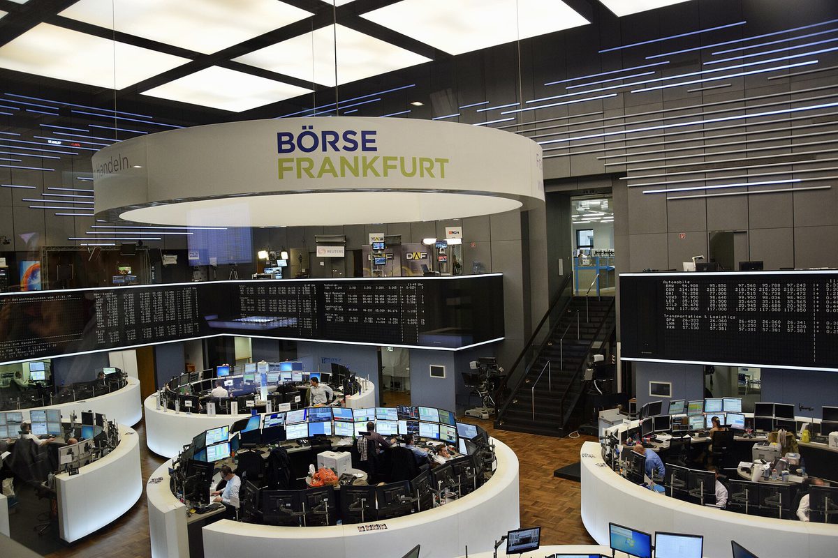
The table compares three periods: a calm period, 2017–2019, and the two crises, September 2008 – March 2009 (the months that followed the bankruptcy of Lehman Brothers, shown in the photograph) and February – April 2020. For each period it gives the average DCC correlation between the S&P 500 and the DAX and the average annualised GARCH volatility of the S&P 500. In the calm period the correlation averages 0.56 and the volatility 13%; in 2008–2009, 0.63 and 51%; in 2020, 0.70 and 58%.
Correlations are higher in crises, but the change is moderate compared with the change in volatility, which roughly quadruples. Most of the rise in covariance during a crisis therefore comes from volatility, a smaller part from the correlation.
The comparison needs care. Forbes and Rigobon (2002) showed that the sample correlation of returns rises mechanically when volatility rises, even if the underlying link between markets is unchanged: a larger common shock dominates the idiosyncratic noise. A higher correlation of raw returns in a crisis is therefore not by itself evidence of contagion. DCC reduces this effect because it measures correlation on the standardised residuals \(z_t\), not on the returns \(r_t\), so the rise in volatility is removed before the correlation is computed.
Average DCC correlation and average annualised S&P 500 volatility in each period
Correlations are higher in crises, but volatility rises far more
Caution Forbes and Rigobon (2002): the sample correlation rises mechanically when volatility rises, even if the link is unchanged; DCC reduces this effect because it works with \(z_t\), not with \(r_t\)
Question for the room ▶ raises a up to 0.022. What happens to the gap between the mean DCC correlation of 2020 and that of the calm period (0.70 − 0.56 = 0.14)?
Answer
It widens to 0.18 (0.73 against 0.55); with a = 0 all three means are 0.575. The sample correlation of the returns (choose it in the box) gives 0.74 and 0.52: it rises mechanically with the volatility (Forbes and Rigobon), while DCC works with the standardised residuals.
Question for the room ▶ raises the multiplier of α up to 2. Does the 2020 correlation still peak before the volatility?
Answer
No: with α doubled the correlation peak, 0.71, is on 12 June 2020, after the volatility peak (139% on 17 March 2020). The larger volatilities of March divide the shocks of those days, so the standardised residuals that drive the DCC recursion are smaller. With the multiplier 0.25 the 2008 volatility peaks only on 2 December 2008 (60%).
The chart has two panels, one for each crisis: June 2008 – June 2009 on the left and December 2019 – August 2020 on the right. Each panel plots the DCC correlation of the S&P 500 and the DAX on the left axis, from 0 to 1, and the annualised GARCH volatility of the S&P 500, in percent, on the right axis, against time.
The two axes make it possible to compare the timing of the two quantities, not their levels. In both panels the volatility line rises and falls steeply, while the correlation line moves in a much narrower range.
In brief
DCC correlation of the S&P 500 and the DAX (left axis) and the GARCH volatility of the S&P 500 (right axis)
The two crises unfolded differently. In 2008 the volatility of the S&P 500 peaked at 90% on 16 October 2008, while the correlation rose slowly, from 0.57 to its maximum of 0.68, reached only on 23 June 2009, months after the volatility peak. The crisis started in the US financial system and spread to Europe gradually.
In 2020 the order was reversed. The correlation jumped to 0.73 on 28 February 2020, before the volatility peak of 109% on 17 March 2020. A global shock, the COronaVIrus Disease 2019 (COVID-19) pandemic, hit both markets on the same days, and the run of joint falls drove the DCC recursion upwards quickly.
Correlations and volatilities need not peak together. A model that ties them, such as a single rolling covariance, would mix the two stories; modelling them separately, as DCC does, shows the difference between a crisis that spreads and a shock that strikes everywhere at once.
In brief
2008: volatility peaks at 90% on 16 October 2008, while the correlation drifts up from 0.57 to 0.68 only by 23 June 2009
2020: the correlation jumps to 0.73 on 28 February 2020, before the volatility peak (109% on 17 March 2020)
a global shock hit both markets on the same days: joint falls drive the DCC recursion
Correlations and volatilities need not peak together: modelling them separately, as DCC does, shows the difference
Step 1 gives persistent GARCH volatilities, with persistence 0.980 and 0.984, which peak together. Step 2 gives \(a + b = 0.9918\) and a likelihood ratio of 131.8 against CCC: the correlation is not constant. Correlations are higher in 2008 and 2020, but the largest change during a crisis is in volatility.
In brief
Step 1: persistent GARCH volatilities that peak together
Step 2: \(a + b = 0.9918\); LR 131.8: the correlation is not constant
Higher correlations in 2008 and 2020, but the largest change is in volatility
Section summary
Two assets show the method; a portfolio usually has more. The next section estimates a single DCC model for five markets of very different kinds, including the Romanian equity market, the leu and Bitcoin, and compares their correlations in calm times and in the 2020 crash.
Five markets: S&P 500, DAX, BET, EUR/RON, Bitcoin
The section fits one DCC model to five assets, two large equity indices, the Romanian BET, the EUR/RON exchange rate and Bitcoin, and compares the average correlations in a calm period and in the COVID-19 crash.
The data are daily log returns on the 2 815 days on which all five markets trade, from 6 January 2015. The BET is the index of the Bucharest Stock Exchange, shown in the photograph. For EUR/RON the reference rate of the National Bank of Romania (BNR), fixed at 13:00 Bucharest time, is used, and for Bitcoin the close of the day in Coordinated Universal Time (UTC). The closing times differ even more than in the first section, so daily correlations of these series carry the asynchronous-trading bias discussed there.
Step 1 gives five GARCH(1,1) models with persistence 0.961 for the S&P 500, 0.965 for the DAX, 0.941 for the BET, 0.985 for EUR/RON and 0.958 for Bitcoin. Step 2 gives \(\hat a = 0.0088\) (SE 0.0019) and \(\hat b = 0.9782\) (SE 0.0062), so the half-life of a correlation shock is 53 days. The likelihood ratio against CCC is 88.5, again far above the 5% critical value of 5.99.
The model has 10 correlation pairs but only one pair of dynamics parameters \((a, b)\) for all of them. The 10 long-run correlations come from \(\bar{\mathbf{Q}}\), the sample correlation of the standardised residuals, so the optimiser of step 2 still works on two parameters only.
Question for the room ▶ shows each asset in turn. Which one has the highest volatility peak, and when?
Answer
Bitcoin: 281% on 13 March 2020. The S&P 500 reaches 121% on 17 March 2020, the DAX 84% on 13 March 2020, the BET 98% on 20 December 2018 (the day on which the DCC hedge ratio reaches 1.00), EUR/RON 13% on 21 May 2025.
Question for the room ▶ raises a up to 0.02. What happens to the range of the S&P 500 – Bitcoin correlation (−0.05 … 0.42)?
Answer
It widens: from −0.33 to 0.62, with the mean still 0.21. With a = 0 the four correlations become constant, equal to Q̄: 0.55, 0.32, 0.21 and −0.07; this is the CCC model, rejected by LR = 88.5.
The chart plots the one-step-ahead DCC correlations of four of the ten pairs on the vertical axis against time, from 2015 to 2026: the S&P 500 and the DAX, the BET and the DAX, the S&P 500 and Bitcoin, and the BET and EUR/RON. A dashed line marks zero, and the shaded band marks the COVID-19 crash, from mid-February to June 2020.
The four lines are clearly separated in level: the S&P 500 and the DAX at the top, the BET and the DAX and the S&P 500 and Bitcoin in the middle, and the BET and EUR/RON around or below zero. Their movements over time are the subject of the next frame.
In brief
One-step-ahead DCC correlations from the five-asset model; shaded: the COVID-19 crash, mid-February–June 2020
The S&P 500 and the DAX have the strongest link, with a mean correlation of 0.54 over 2015–2026. The BET and the DAX have a mean of 0.32 and move between 0.15 and 0.53, the maximum reached in April 2022. The jump of this pair at the start of the 2020 crash is the largest of the four.
The S&P 500 and Bitcoin range from \(-0.05\) to 0.42, the maximum in May 2022, with a mean of 0.21. Before 2020 the correlation stayed low; after 2020 it stayed clearly higher. The diversification benefit of Bitcoin for an equity portfolio has shrunk.
The BET and EUR/RON have a correlation close to zero, with a mean of \(-0.06\). The exchange rate is quoted as lei per euro, so a rise of EUR/RON is a weaker leu, and the small negative correlation means that a weaker leu tends to come with a weaker BET. One feature of the chart is a consequence of the model rather than of the data: all four lines share the same \((a, b)\), so pairs that might adjust at different speeds are forced to the same rhythm. This is the price of the parsimony of DCC.
In brief
S&P 500 and DAX: the strongest link, mean 0.54; BET and DAX: mean 0.32, between 0.15 and 0.53 (April 2022)
S&P 500 and Bitcoin: from \(-\)0.05 to 0.42 (May 2022); mean 0.21
the diversification benefit of Bitcoin shrank after 2020
BET and EUR/RON: close to zero (mean \(-\)0.06); a weaker leu tends to come with a weaker BET, a small negative link
One \((a, b)\) for all pairs: pairs with different speeds are forced to the same rhythm, the price of DCC's parsimony
Question for the room ▶ raises a up to 0.02. What happens to the average correlation in the 2020 crash (0.19)?
Answer
It rises to 0.23, while the calm-period average falls to 0.10. With a = 0 the two matrices are identical (average 0.135): with constant correlations no rise in the crisis can be seen.
The chart shows two heatmaps of the average one-step-ahead DCC correlation matrix of the five assets. The left one averages over the calm period 2017–2019 and the right one over the COVID-19 crash, from mid-February to June 2020, 89 common trading days. Rows and columns are the five assets, each cell holds the average correlation, and the colour scale runs from \(-1\) (blue) to \(1\) (dark red).
The diagonals are ones by construction. The cells for EUR/RON are close to white in both matrices, while the cells linking the BET and Bitcoin with the large equity markets become clearly darker in the crisis panel.
In brief
Average one-step-ahead DCC correlation matrix: 2017–2019 and mid-February–June 2020 (89 common trading days)
The average of the ten pairwise correlations rises from 0.12 in the calm period to 0.19 in the crash. The rise is uneven. For the BET and the DAX the average correlation goes from 0.28 to 0.48, for the S&P 500 and the BET from 0.22 to 0.38, and for the DAX and Bitcoin from 0.10 to 0.27. The S&P 500 and the DAX, already strongly linked, go from 0.55 to 0.64.
The largest rises concern the BET and Bitcoin, the assets weakly linked to the large markets in calm times, which are exactly the assets that were expected to diversify an equity portfolio. When a global shock arrives, these weak links become stronger, and the benefit of diversification shrinks when it matters most.
EUR/RON stays close to zero or slightly negative with all equity markets in both periods, from \(-0.03\) to \(-0.10\). In this set of five assets it is the only one that kept its diversifying role in the crash.
In brief
The average pairwise correlation rises from 0.12 to 0.19
BET and DAX: 0.28 \(\to\) 0.48; S&P 500 and BET: 0.22 \(\to\) 0.38; DAX and Bitcoin: 0.10 \(\to\) 0.27
The largest rises are for the BET and for Bitcoin, which are weakly linked to the large markets in calm times: exactly the assets that were supposed to diversify
EUR/RON stays near zero or slightly negative with all equity markets: the only diversifier in this set
One DCC model describes the ten correlations of five assets with only two dynamics parameters, and the likelihood ratio of 88.5 rejects constant correlation. The correlations of the Romanian market with Europe and of Bitcoin with equities move a great deal. In the 2020 crash the weak links strengthened most, so diversification weakened in the crisis.
In brief
One DCC for 5 assets: 2 dynamics parameters for 10 correlations
Correlations of the Romanian market with Europe and of Bitcoin with equities move a lot
In the 2020 crash the weak links strengthened most: diversification weakens in crises
Section summary
Correlations and volatilities are inputs; risk managers need numbers that can be checked against outcomes. The next section turns the conditional covariance matrix into the VaR of a portfolio and tests it on data that were not used for estimation.
Portfolio VaR 1% with DCC
The section computes the Value at Risk of a portfolio from \(\mathbf{H}_t\), presents the Kupiec and Christoffersen backtests and compares DCC, CCC and a static covariance matrix on an S&P 500 and DAX portfolio from 2015 to 2026.
A portfolio with weights \(\mathbf{w}\) has the return \(r_{p,t} = \mathbf{w}^\top\mathbf{r}_t\), with conditional mean \(\mu_p = \mathbf{w}^\top\boldsymbol{\mu}\) and conditional volatility \(\sigma_{p,t} = \sqrt{\mathbf{w}^\top\mathbf{H}_t\mathbf{w}}\), by (14.1) applied to the conditional covariance matrix. The VaR 1% is the loss that is exceeded with probability 1%, minus the 1% quantile of the portfolio return:
The value of \(q\) depends on the assumed distribution of the standardised portfolio return. Under the Normal distribution \(q = z_{0.01} = -2.326\). Filtered historical simulation (FHS) uses instead the empirical 1% quantile of the past standardised portfolio returns \((r_{p,t} - \mu_p)/\sigma_{p,t}\), which takes the fat tails of the data into account while keeping the volatility dynamics of the model.
Three choices of \(\mathbf{H}_t\) are compared: DCC; CCC, which has GARCH volatilities but a constant correlation; and a static matrix, a single sample covariance matrix used for all days. The static VaR is the same every day, the CCC VaR moves with the volatilities only, and the DCC VaR moves with both volatilities and correlation.
In brief
Portfolio return \(r_{p,t} = \mathbf{w}^\top\mathbf{r}_t\); conditional mean \(\mu_p = \mathbf{w}^\top\boldsymbol{\mu}\) and volatility \(\sigma_{p,t} = \sqrt{\mathbf{w}^\top\mathbf{H}_t\mathbf{w}}\)
VaR 1%
the loss exceeded with probability 1%, \(\mathrm{VaR}_{0.01,t} = -q_{0.01}(r_{p,t}) = -(\mu_p + q\,\sigma_{p,t})\)
Normal: \(q = z_{0.01} = -2.326\)
filtered historical simulation (FHS): \(q\) = the empirical 1% quantile of the past standardised portfolio returns \((r_{p,t} - \mu_p)/\sigma_{p,t}\)
Three choices of \(\mathbf{H}_t\): DCC; CCC (GARCH volatilities with a constant correlation); static (one sample covariance matrix for all days)
Today's forecasts are daily volatilities \(\sigma_1 = 1.5\%\) and \(\sigma_2 = 1.2\%\), the weights are 50% and 50% and the mean is zero. In a calm state with \(\rho_t = 0.3\),(14.1) gives
where \(1.8 = 1.5 \cdot 1.2\) is the product of the volatilities. The portfolio volatility is \(\sigma_p = 1.092\%\) and the Normal VaR 1% is \(2.326 \cdot 1.092 = 2.54\%\).
In a crisis state with \(\rho_t = 0.9\) and the same volatilities, \(\sigma_p = 1.316\%\) and the VaR 1% is 3.06%. The jump of the correlation alone adds about a fifth to the VaR. In a real crisis the volatilities rise as well, so the actual increase is larger.
For a portfolio of 1 million lei, the VaR 1% is about 25.4 thousand lei in the calm case and 30.6 thousand lei in the crisis case. A model with a fixed correlation would report the first number on both days.
In brief
Today's forecasts: \(\sigma_1 = 1.5\%\), \(\sigma_2 = 1.2\%\) (daily), weights 50% and 50%, mean 0
A VaR model is judged by backtesting: comparing its forecasts with the returns that actually followed. A violation (violation) occurs on day \(t\) when \(r_{p,t} < -\mathrm{VaR}_{0.01,t}\), that is when the loss exceeds the VaR. A correct VaR 1% has violations on 1% of the days, and these days occur at random, not in clusters. The two properties are tested separately.
The test of Kupiec (1995) checks the frequency. With \(x\) violations in \(n\) days and observed rate \(\hat p = x/n\), the statistic
compares the likelihood of the observed violations under the nominal rate of 1% with their likelihood under the observed rate. The subscript \(uc\) stands for unconditional coverage. Under a correct model \(LR_{uc}\) follows approximately a \(\chi^2(1)\) distribution, and the model is rejected at 5% if \(LR_{uc} > 3.84\). The test rejects both too many violations, a VaR that is too low, and too few, a VaR that is too high.
In brief
A violation on day \(t\)
\(r_{p,t} < -\mathrm{VaR}_{0.01,t}\)
a correct VaR 1% has violations on 1% of the days, at random times
The test of Christoffersen (1998) checks independence: is a violation more likely on the day after a violation? It compares \(\pi_{11}\), the probability of a violation given a violation yesterday, with \(\pi_{01}\), the probability of a violation given no violation yesterday. For a correct model the two are equal, because a VaR that uses all available information leaves nothing predictable in the violations.
The statistic is built from counts: \(n_{ij}\) is the number of days in state \(j\) that follow a day in state \(i\), where state 1 is a violation and 0 is none. The estimates are \(\hat\pi_{01} = n_{01}/(n_{00}+n_{01})\) and \(\hat\pi_{11} = n_{11}/(n_{10}+n_{11})\), and \(\hat\pi\) is the overall violation rate. The statistic
has a numerator that assumes \(\pi_{01} = \pi_{11}\), no clustering, and a denominator that lets the two probabilities differ. Under independence it follows approximately \(\chi^2(1)\); a small p-value rejects independence.
A backtest is meaningful only out of sample. All parameters are estimated on 2000–2014, 3 712 days, and the filters are then run forward on 2015–2026, 2 893 days, without re-estimating. Each day's VaR uses only information available on the previous day, as it would in practice.
\(n_{ij}\): the number of days in state \(j\) after a day in state \(i\) (1: violation, 0: none); \(\hat\pi_{01} = n_{01}/(n_{00}+n_{01})\), \(\hat\pi_{11} = n_{11}/(n_{10}+n_{11})\)
\(\hat\pi\): the overall violation rate; the numerator assumes \(\pi_{01} = \pi_{11}\) (no clustering); a small \(p\)-value rejects independence
Out-of-sample design
estimate all parameters on 2000–2014 (3 712 days), then run the filters forward on 2015–2026 (2 893 days) without re-estimating
Question for the room ▶ raises ρt up to 1. What is the VaR 1% for ρt = 1?
Answer
3.14%: σp = 0.5 · 1.5 + 0.5 · 1.2 = 1.35%, the largest possible value with these volatilities. With ρt = −0.5 the VaR 1% is 1.60%, about 16.0 thousand lei for 1 million lei.
Question for the room ▶ moves to the levels 2.5% and 5%. At 5%, does any model pass the Christoffersen independence test?
Answer
No: all four have p ≤ 0.0004; the violations come in clusters on the turbulent days. At 2.5% only DCC with FHS passes the Kupiec test (79 violations, a rate of 2.73%, p = 0.433).
Question for the room ▶ moves to the levels 2.5% and 5%. At 5%, what is the violation rate of the static VaR?
Answer
2.83% (82 violations against 145 expected): too few, LRuc = 33.6, p < 0.001. At 1% the static VaR passed the test (0.90%, p = 0.577): it is too high in calm years, which at 1% offsets the violations of the crises and at 5% does not. DCC with FHS has a rate of 4.60% at 5% (p = 0.314).
The chart plots, against time from 2015 to 2026, the daily return in percent of a portfolio with 50% in the S&P 500 and 50% in the DAX, together with minus the VaR 1% of two models: DCC with filtered historical simulation, a line that moves, and the static covariance matrix, a flat line. Red triangles mark the 48 violations of the DCC-FHS model and green triangles the 26 violations of the static model.
The DCC line follows the volatility of the returns: it stays close to the returns in calm years and drops far below them in March 2020, when the returns themselves swing widely. The static line stays at the same level throughout. The green triangles of the static model are concentrated in a few episodes, most visibly in early 2020; the red triangles of DCC are spread across the whole period.
In brief
Daily return of a 50/50 portfolio and minus VaR 1% from DCC with filtered historical simulation and from a static covariance matrix; triangles: violations
With 2 893 out-of-sample days, a correct VaR 1% should have about 29 violations. The table gives, for each model, the number and rate of violations, the Kupiec statistic \(LR_{uc}\) and its p-value, the p-value of the Christoffersen independence test and the number of violations in February – April 2020. DCC with Normal quantiles has 65 violations, a rate of 2.25%, \(LR_{uc} = 33.6\) with a p-value below 0.001 and an independence p-value of 0.003. DCC with FHS has 48 violations, 1.66%, \(LR_{uc} = 10.6\), p-value 0.001, independence p-value 0.008. CCC with Normal quantiles has 57 violations, 1.97%, \(LR_{uc} = 21.4\), p-value below 0.001, independence p-value 0.030. The static model has 26 violations, 0.90%, \(LR_{uc} = 0.3\), p-value 0.577, independence p-value 0.001.
The dynamic models with Normal quantiles have too many violations, because the standardised residuals have fatter tails than the Normal distribution, as the kurtosis of step 1 showed and as Chapter 5 found for single series. FHS replaces \(-2.326\) by the empirical quantile \(q = -2.59\) and brings the rate down to 1.66%, still above 1% but much closer. The remaining violations are also less clustered than for the static model: in February – April 2020 every dynamic model has 4 violations.
The static VaR passes the frequency test, and this is the instructive case. Its 26 violations are close to the expected 29, but 10 of them fall in February – April 2020, and after a violation the next day is also a violation with probability 11.5%, so independence is rejected. The static VaR is 2.95% every day: too high in calm years and far too low in a crash. Its correct average frequency comes from errors in both directions that offset each other. A dynamic VaR adapts in both directions; its remaining problem is the quantile, not the covariance.
In brief
Model
Violations
Rate
\(LR_{uc}\)
\(p\)
\(p\) indep.
Feb–Apr 2020
DCC, Normal
65
2.25%
33.6
\(<\) 0.001
0.003
4
DCC, FHS
48
1.66%
10.6
0.001
0.008
4
CCC, Normal
57
1.97%
21.4
\(<\) 0.001
0.030
4
Static, Normal
26
0.90%
0.3
0.577
0.001
10
Expected: about 29 violations in 2 893 days
Dynamic models with Normal quantiles have too many violations: the residuals have fat tails (Chapter 5); FHS (\(q = -2.59\)) brings the rate down to 1.66%
The static VaR passes the frequency test, but its violations cluster: 10 in February–April 2020 alone, and after a violation the next day is a violation with probability 11.5%
The static VaR is too high in calm years (2.95% every day) and far too low in a crash; a dynamic VaR adapts in both directions
The portfolio volatility is \(\sigma_{p,t} = \sqrt{\mathbf{w}^\top\mathbf{H}_t\mathbf{w}}\) and the VaR 1% is \(-(\mu_p + q\,\sigma_{p,t})\). A VaR is backtested out of sample with the Kupiec test, for the frequency of violations, and the Christoffersen test, for their independence. Dynamic covariances remove most of the clustering of violations; fat tails require a better quantile than the Normal one.
In brief
\(\sigma_{p,t} = \sqrt{\mathbf{w}^\top\mathbf{H}_t\mathbf{w}}\); VaR 1% \(= -(\mu_p + q\,\sigma_{p,t})\)
Backtest out of sample: Kupiec (frequency) and Christoffersen (independence)
Dynamic covariances fix the clustering of violations; fat tails need a better quantile than the Normal
Section summary
The VaR uses the whole matrix \(\mathbf{H}_t\) through one quadratic form. The next application uses its elements separately: the ratio of a covariance to a variance gives the number of units of a hedging asset to sell, and DCC lets this number change every day.
Dynamic hedge ratios
The section derives the minimum-variance hedge ratio and its hedging effectiveness, makes the ratio dynamic with DCC, and compares static, rolling and DCC hedges of the BET with the DAX out of sample.
An investor holds one unit of an asset \(s\), for example Romanian shares represented by the BET, and sells \(h\) units of a hedging asset \(f\), for example a futures contract on the DAX. The hedged return is \(r_{s,t} - h\,r_{f,t}\), and its variance is \(\sigma_s^2 - 2h\,\sigma_{sf} + h^2\sigma_f^2\), where \(\sigma_s^2\) and \(\sigma_f^2\) are the variances of the two returns and \(\sigma_{sf}\) their covariance. Setting the derivative with respect to \(h\) to zero gives the minimum-variance hedge ratio (hedge ratio) of Ederington (1979):
The static version of \(h^*\) is the slope of the ordinary least squares (OLS) regression of \(r_s\) on \(r_f\), because the OLS slope is exactly a covariance divided by a variance. The dynamic version, proposed by Kroner and Sultan (1993), uses the elements of \(\mathbf{H}_t\) from an MGARCH model, \(h_t^* = h_{sf,t}/h_{ff,t}\), and therefore changes with the forecast covariance and variance every day.
The hedging effectiveness (hedging effectiveness) measures the share of variance removed: \(HE = 1 - \Var(r_s - h\,r_f)/\Var(r_s)\). Substituting the constant optimal ratio into the hedged variance gives \(\sigma_s^2(1 - \rho^2)\), so \(HE = \rho^2\). A hedge is only as good as the correlation between the asset and the hedging instrument.
In brief
Hold one unit of asset \(s\) (e.g. Romanian shares, the BET) and sell \(h\) units of a hedging asset \(f\) (e.g. a DAX futures contract)
Take daily volatilities \(\sigma_s = 1.2\%\) and \(\sigma_f = 1.0\%\) and a correlation \(\rho = 0.8\). The covariance is \(\sigma_{sf} = \rho\,\sigma_s\sigma_f = 0.8 \cdot 1.2 \cdot 1.0 = 0.96\), and by (14.12) the hedge ratio is \(h^* = 0.96/1 = 0.96\): the investor sells 0.96 units of \(f\) for each unit of \(s\).
The hedging effectiveness is \(\rho^2 = 0.64\), so the hedge removes 64% of the variance. The volatility of the hedged position is \(\sigma_s\sqrt{1 - \rho^2} = 0.72\%\) instead of 1.2%. Volatility falls less than variance, by 40% instead of 64%, because it is the square root.
If tomorrow the DCC model forecasts \(\rho_t = 0.5\) and \(\sigma_{f,t} = 2\%\), with \(\sigma_s\) unchanged, the ratio becomes \(0.5 \cdot 1.2/2 = 0.3\). Both the lower correlation and the higher volatility of the hedging asset reduce the number of units to sell, and the position must be adjusted.
Step 2: \(h^* = \sigma_{sf}/\sigma_f^2 = 0.96/1 = 0.96\): sell 0.96 units of \(f\) per unit of \(s\)
Step 3: \(HE = \rho^2 = 0.64\); the hedged volatility is \(\sigma_s\sqrt{1 - \rho^2} = 0.72\%\) instead of 1.2%
If tomorrow DCC forecasts \(\rho_t = 0.5\) and \(\sigma_{f,t} = 2\%\), the hedge ratio becomes \(0.5 \cdot 1.2/2 = 0.3\): the position must be adjusted
Question for the room Set ρ = −0.8. What are h* and HE?
Answer
h* = −0.96: buy 0.96 units of f per unit of s; HE = ρ2 = 0.64, as for ρ = 0.8. With ρ = 1 the volatility of the hedged position is 0 (h* = 1.2).
Question for the room Is there a window (60–500 days) for which rolling OLS removes more risk than DCC?
Answer
No: the best result is 18.6%, with 80 days, below 19.1% for DCC; 300 days give only 17.0%. The choice of the window moves the result by more than a percentage point, and DCC needs no such choice.
Question for the room ▶ lengthens the OLS window up to 500 days. Does rolling OLS then remove more risk than DCC (19.1%)?
Answer
No: between 17.0% (300 days) and 18.0% (500 days). With a = 0 in the DCC the effectiveness falls to 15.5%, still above the static ratio (13.6%): the correlation is then constant, but the ratio q̄ σBET,t/σDAX,t still follows the GARCH volatilities.
The chart plots three hedge ratios, in units of DAX sold per unit of BET, against time from 2015 to 2026: the DCC ratio \(h_t = \hat\rho_t\hat\sigma_{BET,t}/\hat\sigma_{DAX,t}\), the rolling OLS slope over the previous 250 days and the static OLS ratio estimated on 2005–2014, a dashed horizontal line. The data are daily returns on common trading days of the two markets since 2005, and all parameters of the DCC model are estimated on 2005–2014.
The DCC ratio is the most volatile line, with short spikes, the highest at the end of 2018. The rolling OLS ratio moves in steps, and its large jump in early 2020 lasts about a year, the length of its window. The static line lies above both dynamic ratios for most of the period.
In brief
Daily returns on common trading days since 2005; all parameters estimated on 2005–2014; DCC: \(h_t = \hat\rho_t\hat\sigma_{BET,t}/\hat\sigma_{DAX,t}\); rolling OLS: the slope over the previous 250 days
The static ratio of 0.51 reflects the period 2005–2014, which includes the 2008 crisis, when the BET and the DAX were closely linked. After 2015 the DCC ratio averages 0.29 and ranges from 0.07 to 1.00, the maximum reached on 20 December 2018. The static ratio thus over-hedges in most of the later period.
The hedging effectiveness out of sample, over 2 893 days, is 13.6% for the static ratio, 18.0% for the rolling OLS ratio and 19.1% for the DCC ratio. The dynamic ratios remove more risk, and DCC does so without the choice of a window.
All three values are modest. The DCC correlation between the BET and the DAX averages 0.32 since 2015, so \(\rho^2\) is about a tenth, and no ratio can remove much of the variance of the BET with the DAX. A daily DCC ratio also implies daily rebalancing and trading costs, which are not counted in these figures; after costs, the advantage of DCC over the static ratio would be smaller.
In brief
The static ratio 0.51 reflects 2005–2014, which includes the 2008 crisis; after 2015 the DCC ratio averages 0.29, from 0.07 to 1.00 (20 December 2018)
Hedging effectiveness out of sample (2 893 days): static 13.6%, rolling OLS 18.0%, DCC 19.1%
the dynamic ratios remove more risk, and DCC does so without choosing a window
All effectiveness values are modest: the BET–DAX DCC correlation averages 0.32 since 2015, so \(\rho^2\) is small
a daily DCC ratio also implies daily trading costs, which are not counted here
The dynamic minimum-variance hedge ratio is \(h_t^* = h_{sf,t}/h_{ff,t} = \rho_t\sigma_{s,t}/\sigma_{f,t}\), and the hedging effectiveness is the share of variance removed. For the BET hedged with the DAX, DCC removes 19.1% of the variance out of sample, against 13.6% for the static ratio. A hedge must be judged out of sample and after trading costs.
BET with DAX: DCC 19.1% against static 13.6% out of sample
Judge a hedge out of sample and after trading costs
Section summary
The applications have shown what the conditional covariance matrix adds in practice. The next section places the chapter among the earlier ones and lists what the DCC model cannot do.
Links with other chapters and limits
The section links multivariate GARCH models with univariate GARCH, VAR models and cointegration, and lists the main limits of DCC and the extensions that address them.
Every MGARCH model contains univariate GARCH models: the diagonal of \(\mathbf{H}_t\) consists of conditional variances, as in Chapter 5. In DCC the link is literal, since the univariate GARCH models are step 1 of the estimation.
A VAR model of Chapter 6 describes spillovers in the mean, for example whether yesterday's DAX return helps to forecast today's BET return. A BEKK model with a full matrix \(\mathbf{A}\) describes spillovers in the variance, whether yesterday's shock to the DAX raises today's variance of the BET. The two combine naturally: a VAR for the mean \(\boldsymbol{\mu}_t\) and an MGARCH model for \(\mathbf{H}_t\).Diebold and Yilmaz (2009) built spillover indices from the variance decompositions of a VAR.
Cointegration, from Chapter 7, is a long-run link between price levels; correlation is a short-run link between returns. The two are distinct. Two prices can be highly correlated from day to day and still drift apart for ever, or be cointegrated with a low daily correlation. A vector error correction model (VECM) can carry DCC errors, with equilibrium in the mean and dynamic correlation in the shocks.
a VAR models spillovers in the mean (e.g. whether yesterday's DAX return helps to forecast today's BET return)
BEKK with a full \(\mathbf{A}\) models spillovers in the variance
the two combine: a VAR for \(\boldsymbol{\mu}_t\) and an MGARCH for \(\mathbf{H}_t\); spillover indices from variance decompositions Diebold and Yilmaz (2009)
DCC buys its parsimony with restrictions. A single pair \((a, b)\) drives all correlations, so pairs that adjust at different speeds are forced to the same rhythm, as the five-market model showed. The volatilities come from separate univariate GARCH models, so DCC has no spillovers between volatilities. And the Normal quasi-likelihood says nothing about the tails: for risk measures, Student \(t\) innovations or filtered historical simulation are needed, as the backtest showed.
Correlations also react asymmetrically: they rise more after joint falls than after joint rises, which the asymmetric DCC of Cappiello, Engle and Sheppard (2006) captures. For hundreds of assets even DCC becomes hard to handle, because the sample matrix \(\bar{\mathbf{Q}}\) is noisy and the step-2 likelihood requires inverting a large matrix every day; factor models, composite likelihood and shrinkage of \(\bar{\mathbf{Q}}\) are the usual answers.
Finally, correlation measures linear dependence only. Two assets can have a moderate correlation and still crash together much more often than a Normal model implies. Joint extremes are described by copulas and by tail dependence; Longin and Solnik (2001) studied the correlation of international equity markets in the tails directly.
Hundreds of assets: factor models, composite likelihood and shrinkage of \(\bar{\mathbf{Q}}\)
Correlation is linear dependence; for joint extremes see copulas and tail dependence Longin and Solnik (2001)
Section summary
DCC is the workhorse of multivariate volatility because it splits a hard problem into univariate GARCH models and a correlation recursion with two parameters. Its limits, a common speed for all pairs, no volatility spillovers and Normal tails, are known and have standard extensions.
Possible contribution of AI
The section describes what an artificial intelligence (AI) assistant can do in multivariate volatility modelling and what must be checked every time.
An AI assistant can quickly write a first version of the code the chapter needs: the DCC correlation likelihood, a BEKK filter or the Kupiec test. It can also give a second explanation, phrased differently, of the ideas that are harder on first reading, such as the decomposition \(\mathbf{D}_t\mathbf{R}_t\mathbf{D}_t\), correlation targeting or the formula of the hedge ratio.
The greatest benefit comes in exploration: DCC models for many pairs at once, such as the markets of Central and Eastern Europe (CEE), sectors or currencies, and a first look at how their correlations behaved in crises. The prompt on the slide is an example of a precise request: it names the data, the alignment on common trading days, the two steps of estimation, correlation targeting and the out-of-sample comparison with static OLS. The more of these choices the request fixes, the easier the result is to check.
In brief
Code
a first draft of the DCC likelihood, of a BEKK filter, of a Kupiec test
Explanation
a second explanation of \(\mathbf{D}_t\mathbf{R}_t\mathbf{D}_t\), of correlation targeting, of the hedge-ratio formula
Exploration
DCC for many pairs (CEE markets, sectors, currencies) and their behaviour in crises
Example prompt
Write Python code that fits a GARCH(1,1) to daily BET and DAX log returns on common trading days, estimates a DCC(1,1) model by two-step maximum likelihood with correlation targeting, plots the dynamic hedge ratio and compares its out-of-sample hedging effectiveness with static OLS.
The first check is the library. The arch package has no DCC model, so an answer that calls arch_model(..., vol='DCC') has invented a function. The second is timing: \(\mathbf{Q}_t\) must use \(\mathbf{z}_{t-1}\), not \(\mathbf{z}_t\); otherwise the VaR and the hedge ratio use tomorrow's information, and the backtest looks better than any real forecast could. The third is the rescaling (14.8): every \(\mathbf{R}_t\) must have ones on the diagonal and correlations below one in absolute value.
The other checks concern data and evaluation. Prices must be aligned on common trading days before returns are computed, and asynchronous closes must be kept in mind. Models must be estimated on one period and tested on another. A simple test of any DCC code is a simulation: generate data from a DCC with known \((a, b)\) and check that the code recovers them. Every reference suggested by an assistant must exist, and its digital object identifier (DOI) must be checked.
In brief
The library: arch has no DCC model; an AI answer that calls arch_model(..., vol='DCC') has invented it
The timing: \(\mathbf{Q}_t\) must use \(\mathbf{z}_{t-1}\), not \(\mathbf{z}_t\); otherwise the VaR and the hedge use tomorrow's information
The rescaling: \(\rho_{ij,t} = q_{ij,t}/\sqrt{q_{ii,t}q_{jj,t}}\), and every \(\mathbf{R}_t\) must have ones on the diagonal and \(|\rho| < 1\)
The calendars: align prices on common trading days before computing returns; watch asynchronous closes
The evaluation: estimate on one period and test on another; simulate a DCC with known \((a, b)\) and check that the code recovers it
Every cited reference: it must exist; check the DOI
Section summary
An assistant shortens the writing of code but does not replace the checks specific to multivariate models: the timing of the recursion, the validity of each correlation matrix, the alignment of calendars and an honest out-of-sample evaluation.
Summary
The summary gathers the chapter's main ideas, the formulas to remember and the self-assessment questions.
Portfolio risk, hedging and contagion depend on the conditional covariance matrix \(\mathbf{H}_t\), which changes over time. VEC is the most general linear model but has far too many parameters; BEKK is positive definite by construction and measures volatility spillovers. CCC and DCC split \(\mathbf{H}_t = \mathbf{D}_t\mathbf{R}_t\mathbf{D}_t\) and are estimated in two steps, and step 2 of DCC needs only \((a, b)\) whatever the number of assets.
The data show that real correlations move: through the integration of the Romanian market with Europe, through crises and through the arrival of Bitcoin as a risk asset. Constant correlation is rejected for the S&P 500 and the DAX and for the five-market model. The applications turn \(\mathbf{H}_t\) into a portfolio VaR 1%, judged by backtesting, and into dynamic hedge ratios, judged out of sample.
In brief
Portfolio risk, hedging and contagion depend on time-varying covariances \(\mathbf{H}_t\)
VEC is general but has too many parameters; BEKK is positive definite by construction and measures spillovers
CCC and DCC split \(\mathbf{H}_t = \mathbf{D}_t\mathbf{R}_t\mathbf{D}_t\) and are estimated in two steps; DCC needs only \((a, b)\) in step 2
Real correlations move: integration, crises, new assets; constant correlation is rejected
Applications: portfolio VaR 1% with backtesting; dynamic hedge ratios judged out of sample
The table gathers the chapter's formulas: the conditional correlation (14.3); the BEKK model (14.6); the decomposition (14.7) used by CCC and DCC; the DCC recursion with its rescaling (14.8); the half-life \(\ln 0.5/\ln(a + b)\); the portfolio VaR 1% (14.10); and the hedge ratio (14.12) with the hedging effectiveness.
The formulas form a chain. The decomposition separates what univariate GARCH models already handle from the correlations; the DCC recursion makes the correlations dynamic; the half-life summarises their persistence; and the VaR and the hedge ratio turn the resulting \(\mathbf{H}_t\) into decisions.
The first question applies the parameter count of the diagonal BEKK: for \(N = 3\) the constant matrix has \(N(N+1)/2 = 6\) distinct elements and the diagonals of \(\mathbf{A}\) and \(\mathbf{B}\) have \(2N = 6\), so 12 in total. The second applies (14.3) and the positive-definiteness condition: with \(h_{11} = 1\),\(h_{22} = 4\) and \(h_{12} = 1.2\) the correlation is \(1.2/\sqrt{4} = 0.6\), and the determinant \(1 \cdot 4 - 1.44\) is positive, so the matrix is positive definite.
The third question is one step of (14.8) with \(a = 0.02\),\(b = 0.97\),\(\bar q_{12} = 0.4\) and \(z_{t-1} = (1, -1)\). The weight of the long-run term is 0.01 and the cross-product of the residuals is \(-1\), so
The first question applies (14.12): with \(\sigma_s = 2\%\),\(\sigma_f = 1\%\) and \(\rho = 0.5\) the hedge ratio is \(0.5 \cdot 2/1 = 1\) and the hedging effectiveness \(\rho^2 = 0.25\). The second concerns backtesting: 26 violations in 2 500 days are close to the expected 25, so the frequency test is passed, but 10 violations in a single month are a cluster that the independence test rejects, and they show a VaR that does not adapt to crises, like the static VaR of the S&P 500 and DAX portfolio.
The third question returns to asynchronous trading: news from New York reaches Bucharest only on the next trading day, so the daily returns of the same calendar day do not match and the daily correlation is lower than the weekly one. The fourth concerns contagion: a higher correlation of returns in a crisis does not prove contagion by itself, because higher volatility raises the sample correlation mechanically (Forbes and Rigobon, 2002); the comparison must use correlations of standardised residuals. Chapter 15 reviews the whole course.
In brief
Question: \(\sigma_s = 2\%\), \(\sigma_f = 1\%\), \(\rho = 0.5\). What are the hedge ratio and the hedging effectiveness?
Question: a VaR 1% has 26 violations in 2 500 days, 10 of them in one month. Is it a good VaR?
Answer: the frequency is fine (expected 25), but the violations cluster: it fails the independence test and does not adapt to crises
Question: why can the daily correlation of the S&P 500 and the BET be lower than the weekly one?
Answer: asynchronous trading: news from New York reaches Bucharest the next day, so daily returns of the same day do not match
Question: does a higher correlation in a crisis prove contagion?
Answer: not by itself: higher volatility raises the sample correlation mechanically Forbes and Rigobon (2002); compare correlations of standardised residuals
Next: Chapter 15, review and exam preparation; check yourself with the quiz of this chapter
Section summary
The chapter extended volatility modelling from one series to several. The central object is the conditional covariance matrix, and the central idea of DCC is to model volatilities and correlations separately, with univariate GARCH models for the first and a two-parameter recursion for the second. On real data the correlations move, rise in crises most for the weakest links, and change the risk of a portfolio and the size of a hedge.
Aielli, G. P. (2013). Dynamic conditional correlation: On properties and estimation. Journal of Business & Economic Statistics, 31(3), 282–299. doi:10.1080/07350015.2013.771027
Bauwens, L., Laurent, S., & Rombouts, J. V. K. (2006). Multivariate GARCH models: A survey. Journal of Applied Econometrics, 21(1), 79–109. doi:10.1002/jae.842
Bollerslev, T. (1986). Generalized autoregressive conditional heteroskedasticity. Journal of Econometrics, 31(3), 307–327. doi:10.1016/0304-4076(86)90063-1
Bollerslev, T. (1990). Modelling the coherence in short-run nominal exchange rates: A multivariate generalized ARCH model. The Review of Economics and Statistics, 72(3), 498–505. doi:10.2307/2109358
Bollerslev, T., Engle, R. F., & Wooldridge, J. M. (1988). A capital asset pricing model with time-varying covariances. Journal of Political Economy, 96(1), 116–131. doi:10.1086/261527
Cappiello, L., Engle, R. F., & Sheppard, K. (2006). Asymmetric dynamics in the correlations of global equity and bond returns. Journal of Financial Econometrics, 4(4), 537–572. doi:10.1093/jjfinec/nbl005
Christoffersen, P. F. (1998). Evaluating interval forecasts. International Economic Review, 39(4), 841–862. doi:10.2307/2527341
Diebold, F. X., & Yilmaz, K. (2009). Measuring financial asset return and volatility spillovers, with application to global equity markets. The Economic Journal, 119(534), 158–171. doi:10.1111/j.1468-0297.2008.02208.x
Ederington, L. H. (1979). The hedging performance of the new futures markets. The Journal of Finance, 34(1), 157–170. doi:10.1111/j.1540-6261.1979.tb02077.x
Engle, R. F. (2002). Dynamic conditional correlation: A simple class of multivariate generalized autoregressive conditional heteroskedasticity models. Journal of Business & Economic Statistics, 20(3), 339–350. doi:10.1198/073500102288618487
Engle, R. F., & Kroner, K. F. (1995). Multivariate simultaneous generalized ARCH. Econometric Theory, 11(1), 122–150. doi:10.1017/S0266466600009063
Forbes, K. J., & Rigobon, R. (2002). No contagion, only interdependence: Measuring stock market comovements. The Journal of Finance, 57(5), 2223–2261. doi:10.1111/0022-1082.00494
Huang, C., & Petukhina, A. (2022). Applied Time Series Analysis and Forecasting with Python. Springer. doi:10.1007/978-3-031-13584-2
Kroner, K. F., & Sultan, J. (1993). Time-varying distributions and dynamic hedging with foreign currency futures. Journal of Financial and Quantitative Analysis, 28(4), 535–551. doi:10.2307/2331164
Kupiec, P. H. (1995). Techniques for verifying the accuracy of risk measurement models. The Journal of Derivatives, 3(2), 73–84. doi:10.3905/jod.1995.407942
Longin, F., & Solnik, B. (2001). Extreme correlation of international equity markets. The Journal of Finance, 56(2), 649–676. doi:10.1111/0022-1082.00340
Silvennoinen, A., & Teräsvirta, T. (2009). Multivariate GARCH models. In T. G. Andersen et al. (Eds.), Handbook of Financial Time Series (pp. 201–229). Springer. doi:10.1007/978-3-540-71297-8_9
Tse, Y. K. (2000). A test for constant correlations in a multivariate GARCH model. Journal of Econometrics, 98(1), 107–127. doi:10.1016/S0304-4076(99)00080-9
The daily log returns (in %) of the chapter’s samples, on the common trading days (S&P 500, DAX, BET, EUR/RON, Bitcoin; data/market, EODHD), are not revised and reproduce the numbers of the lecture exactly. The estimates come from the chapter’s code: the GARCH(1,1) models of step 1 (arch package) and the parameters (a, b) of step 2 with their standard errors, for the S&P 500 and the DAX (2000–2026), for the five-asset panel (since 2015), for the 2000–2014 estimation sample of the VaR and for the 2005–2014 sample of the hedge. The browser runs the recursions again: the GARCH variance filter with the given parameters, the DCC recursion, the rolling correlations and slopes, the correlation log-likelihood, the VaR and the Kupiec and Christoffersen tests. Variants that do not appear in the lecture (other windows, other values of a and b, another α of step 1 with the same persistence, other VaR levels, k-day returns, the forecasts without new shocks, the quarterly means) are extra runs of the chapter’s code on the same data; the charts of the “Worked example” boxes, “Asynchronous trading and the bias of daily correlations”, “Two conditions on Hₜ”, “The curse of dimensionality”, “Reading a and b”, “Step 1: two univariate GARCH models”, “Step 2: the estimated DCC”, “Correlations in crises”, “A five-asset DCC”, “Interpreting the backtest” and “Interpreting the hedge ratios” are extra charts for slides that give only numbers.
References
Aielli, G. P. (2013). Dynamic conditional correlation: On properties and estimation. Journal of Business & Economic Statistics, 31(3), 282–299. https://doi.org/10.1080/07350015.2013.771027
Bauwens, L., Laurent, S., & Rombouts, J. V. K. (2006). Multivariate GARCH models: A survey. Journal of Applied Econometrics, 21(1), 79–109. https://doi.org/10.1002/jae.842
Bollerslev, T. (1990). Modelling the coherence in short-run nominal exchange rates: A multivariate generalized ARCH model. The Review of Economics and Statistics, 72(3), 498–505. https://doi.org/10.2307/2109358
Bollerslev, T., Engle, R. F., & Wooldridge, J. M. (1988). A capital asset pricing model with time-varying covariances. Journal of Political Economy, 96(1), 116–131. https://doi.org/10.1086/261527
Cappiello, L., Engle, R. F., & Sheppard, K. (2006). Asymmetric dynamics in the correlations of global equity and bond returns. Journal of Financial Econometrics, 4(4), 537–572. https://doi.org/10.1093/jjfinec/nbl005
Christoffersen, P. F. (1998). Evaluating interval forecasts. International Economic Review, 39(4), 841–862. https://doi.org/10.2307/2527341
Diebold, F. X., & Yilmaz, K. (2009). Measuring financial asset return and volatility spillovers, with application to global equity markets. The Economic Journal, 119(534), 158–171. https://doi.org/10.1111/j.1468-0297.2008.02208.x
Engle, R. F. (2002). Dynamic conditional correlation: A simple class of multivariate generalized autoregressive conditional heteroskedasticity models. Journal of Business & Economic Statistics, 20(3), 339–350. https://doi.org/10.1198/073500102288618487
Forbes, K. J., & Rigobon, R. (2002). No contagion, only interdependence: Measuring stock market comovements. The Journal of Finance, 57(5), 2223–2261. https://doi.org/10.1111/0022-1082.00494
Kroner, K. F., & Sultan, J. (1993). Time-varying distributions and dynamic hedging with foreign currency futures. Journal of Financial and Quantitative Analysis, 28(4), 535–551. https://doi.org/10.2307/2331164
Kupiec, P. H. (1995). Techniques for verifying the accuracy of risk measurement models. The Journal of Derivatives, 3(2), 73–84. https://doi.org/10.3905/jod.1995.407942
Longin, F., & Solnik, B. (2001). Extreme correlation of international equity markets. The Journal of Finance, 56(2), 649–676. https://doi.org/10.1111/0022-1082.00340
Silvennoinen, A., & Teräsvirta, T. (2009). Multivariate GARCH models. In T. G. Andersen et al. (Eds.), Handbook of Financial Time Series (pp. 201–229). Springer. https://doi.org/10.1007/978-3-540-71297-8_9


 Applied Time Series Analysis with Python
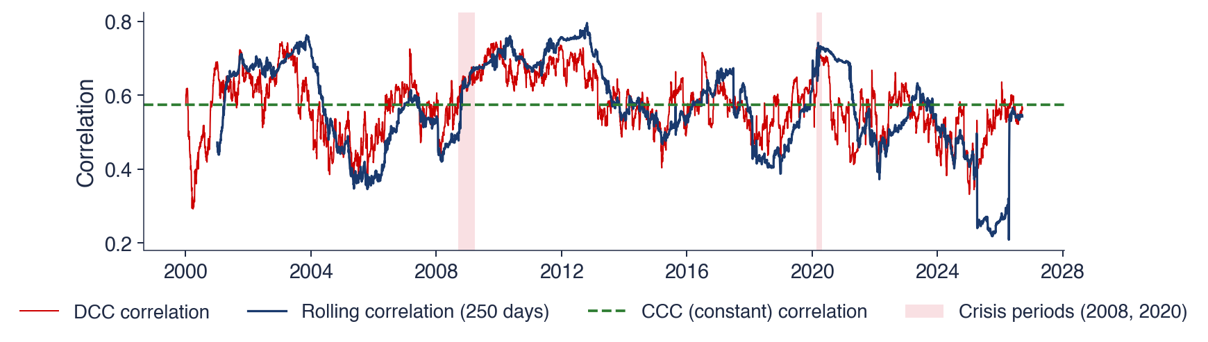
 TSA_ch14_correlations