Bucharest University of Economic Studies IDA Institute Digital Assets Blockchain Research Center AI4EFin Artificial Intelligence for Energy Finance Romanian Academy, Institute for Economic Forecasting MSCA Digital Finance
The chapter starts from a question about shocks: when a series rises over time, does the effect of today's shock die out or does it last for ever? The answer fixes the treatment of the series, detrending or differencing, and the width of forecast intervals at long horizons. The route has three stages. The first defines the two kinds of trend, integrated processes \(I(d)\) and spurious regression. The second presents the unit-root tests, Dickey–Fuller, ADF and Phillips–Perron, the KPSS stationarity test and the effect of structural breaks. The third builds ARIMA\((p,d,q)\) models: identification, estimation, diagnostics and forecasting.
The chapter uses the notions of Chapter 1, stationarity, the random walk and the difference operator, and the ARMA models of Chapter 2. Seminar 3 precedes the lecture and introduces the same tests on short examples.
In brief
Question: when a series drifts upwards, is the shock of today temporary or permanent, and how should we forecast it?
the answer decides whether we detrend or difference, and how wide our forecast intervals are
Route of the chapter
deterministic and stochastic trends; integrated processes \(I(d)\); spurious regression
The core textbook is Huang and Petukhina (2022), chapters 4 and 5, on ARIMA models and non-stationarity. The companion textbook, Hyndman and Athanasopoulos (2021), free online, covers ARIMA models in chapter 9, with an emphasis on forecasting and automatic selection. For the asymptotic theory of unit roots, the reference is Hamilton (1994), chapters 15–17, and the ARIMA methodology is set out in Box, Jenkins and Reinsel (2008).
The ADF, KPSS and Zivot–Andrews tests and ARIMA estimation are available in the Python library statsmodels; the Phillips–Perron test can be written directly from its formula, given in section 4. The lecture notebook reproduces the charts and tables of the chapter.
Most macroeconomic and financial series rise over time: real gross domestic product (GDP), the price level, the exchange rate, stock indices. Their mean is not constant, so the stationary tools of the previous chapters do not apply to them directly. The question of the chapter is what kind of trend these series have. If the trend is a fixed line, a shock moves the series away from the line only temporarily. If the trend is stochastic, every shock stays in the level of the series for ever. The two cases call for different treatments: in the first the trend is removed, in the second the series is differenced.
The difference has direct practical consequences. A trend-stationary model estimated on US real GDP up to 2007Q4 expected output to return to its pre-crisis line. The return never came: in 2026Q2, observed GDP was about 30 log points below that forecast, while the half-width of the 95% interval was only 8 points. The difference-stationary model also misses, by about 25 points, but its interval, with a half-width of 23, at least signals that the uncertainty is large. The nature of the trend also decides whether a regression between two trending series makes sense: the question of Yule (1926) in the epigraph concerns exactly the correlations found between series that evolve as sums of shocks.
The chapter first treats the difference between the two kinds of trend and spurious regression. It then turns to the tests that decide between them, augmented Dickey–Fuller (ADF), Phillips–Perron (PP) and KPSS, with their limits in short samples and in the presence of structural breaks. The last part builds the ARIMA\((p,d,q)\) models, which add differencing to the ARMA models of Chapter 2, and uses them to forecast Romanian GDP, inflation and the EUR/RON exchange rate.
US real GDP (100 ln) and two forecasts made in 2007Q4: a trend-stationary model (linear trend with AR(2) errors) and a difference-stationary model (ARIMA(1,1,0) with drift), with their 95% intervals; on the right, the outcome minus the forecast, in log points.
What you will be able to do
Distinguish trend-stationary from difference-stationary series and explain the effect of a shock in each case.
Recognise a spurious regression from \(t\),\(R^2\) and the Durbin–Watson statistic and explain why it arises.
Apply the ADF, Phillips–Perron and KPSS tests with suitable deterministic terms and lag lengths and interpret them jointly.
Explain how a structural break can mimic a unit root and how the Zivot–Andrews test searches for it.
Identify, estimate and check an ARIMA\((p,d,q)\) model and derive the width of its forecast intervals.
Evaluate critically the output of an automatic ARIMA selection.
Chapter plan
Deterministic and stochastic trendsTrend-stationary and difference-stationary series, integrated processes, the unit root and spurious cycles.
Spurious regressionYule's nonsense correlations, the Granger–Newbold simulation, Phillips's theory and an example on real data.
The Dickey–Fuller testThe \(\tau\) statistic, the three regressions, critical values, the augmented test, lag choice, power and the order of integration.
SummaryKey ideas and formulas and the self-assessment.
Deterministic and stochastic trends
A trending series can be described in two ways. The first is a fixed line plus stationary deviations from it: a deterministic trend. The second is a cumulative sum of shocks, possibly with a drift: a stochastic trend. On a chart the two look almost the same; they differ in the effect of a shock, in the long-run variance and in the correct treatment. The section defines the two models, integrated processes and the unit root, then shows what happens when a series receives the wrong treatment.
Question for the room The ▶ button moves the end of the sample on which the dashed straight lines of all four panels are fitted. Where is GDP in 2026Q2 relative to a line fitted on the data up to 2008Q3?
Answer
Far below it: the line fitted up to 2008Q3 has a slope of 1.56% per quarter, and GDP in 2026Q2 is 76 log points (100 × the difference of logs) below its extension. On the full sample the slope is 0.80% per quarter (about 3.2% a year), and the largest deviation, 17.5 log points, occurs in 2008Q3. After the 2009 recession GDP did not return to the earlier line: an argument for a stochastic trend, not for a fixed line plus noise.
The chart brings together four Romanian and international series observed since 2000. Top left is the logarithm of Romania's quarterly real GDP, seasonally adjusted, together with the line fitted by least squares. Top right is the logarithm of the harmonised index of consumer prices (HICP), monthly, with base 2015 = 100. Bottom left is the daily EUR/RON rate, the reference rate of the National Bank of Romania (BNR), from July 2005. Bottom right are the logarithms of the daily prices of the BET and S&P 500 indices, each minus its value in 2000, so that both start at zero.
None of the series fluctuates around a constant mean. In the terms of Chapter 1, all are non-stationary: their mean depends on time. The shape of the growth differs, however. GDP follows a line from which it departs in long episodes, the HICP rises fast at first and more slowly after 2005, the exchange rate has rare jumps followed by periods of stability, and the BET collapses in 2008–2009 and then recovers slowly.
In brief
Romanian real GDP (Eurostat, seasonally adjusted) and HICP (Eurostat); EUR/RON, the BNR reference rate; BET and S&P 500 log prices, daily since 2000
None of them has a constant mean: Chapter 1 called them non-stationary
The figures give the order of magnitude of the trends. Real GDP grows on average by 0.80% per quarter, about 3.2% per year, but departs from the fitted line by up to 18%. Consumer prices have risen 7.2-fold since 2000. The EUR/RON rate went from 3.60 to 5.26 lei. The logarithm of the BET rose by 426 log points (that is, \(100\Delta\ln\)) and that of the S&P 500 by 166 points, up to 18 September 2026.
The 2009 recession illustrates the question of the chapter. After the fall, Romanian GDP grew again, but it is not clear whether it returned to the old line or started on a new one, parallel and lower. The first case corresponds to a temporary shock, the second to a permanent one.
Two models can produce such charts. The first is a fixed line plus stationary noise, a deterministic trend. The second is a random walk with drift, a stochastic trend. The next two frames define them formally and compare their properties.
In brief
GDP grows by 0.80% per quarter on average (about 3.2% per year), but it strays from the straight line by up to 18%
the 2009 recession: did GDP come back to the old line, or did it start a new one?
Consumer prices: \(\times\)7.2 since 2000; EUR/RON: from 3.60 to 5.26 lei; BET: \(+426\) log points, S&P 500: \(+166\) log points (to 18 September 2026)
Two models can produce such pictures
a fixed line plus stationary noise (deterministic trend)
In (3.1),\(\alpha\) is the intercept, \(\beta\) the slope, that is the average change per period, and \(u_t\) a stationary process, for example an AR(1) \(u_t = \phi u_{t-1} + \varepsilon_t\) with \(|\phi| < 1\) (Chapter 2). The mean \(E[y_t] = \alpha + \beta t\) depends on time, so \(y_t\) is not stationary, but the variance \(\mathrm{Var}(y_t) = \mathrm{Var}(u_t)\) is constant and \(y_t - \alpha - \beta t\) is stationary.
A shock \(\varepsilon_t\) moves the series away from the line only temporarily. With AR(1) errors, its effect after \(h\) periods is \(\phi^h\), which goes to zero geometrically. Long-run forecasts therefore return to the line \(\alpha + \beta(T+h)\), and the forecast-error variance converges to \(\mathrm{Var}(u_t)\): forecast intervals have a bounded width. The correct treatment is to estimate the trend by ordinary least squares (OLS) and to model the residuals as an ARMA process.
In brief
Definition: \(y_t = \alpha + \beta t + u_t\), with \(u_t\) a stationary process (for example a stationary AR(1), Chapter 2)
\(\alpha\): the intercept; \(\beta\): the slope, the average change per period; \(t\): the time index
\(y_t\) is trend-stationary (TS): stationary after subtracting the line \(\alpha + \beta t\)
Here \(\beta\) is the drift, the average change per period. By repeated substitution, \(y_t = y_0 + \beta t + \sum_{i=1}^{t} u_i\), where \(y_0\) is the initial value. The series has two trend components: the deterministic term \(\beta t\), which comes from the drift, and the cumulative sum of shocks \(\sum_{i \le t} u_i\), called the stochastic trend.
The mean is the same as in (3.1),\(y_0 + \beta t\), but the variance grows with time: for a random walk, with \(u_t\) white noise of variance \(\sigma^2\),\(\mathrm{Var}(y_t) = t\sigma^2\) (Chapter 1). Every shock enters the cumulative sum and stays in the level for ever; there is no line to which the series returns. As a consequence, forecast intervals widen without limit as the horizon grows. The correct treatment is to difference the series and to model \(\Delta y_t\) as ARMA, that is the ARIMA model of section 6.
Question for the room The ▶ button raises φ from 0 to 1. What is left, at the end of the sample, of the +6 shock in the trend-stationary series?
Answer
For φ < 1, almost nothing: 6φ⁹⁹ is 1.5 · 10⁻⁹ at φ = 0.8 and 0.04 at φ = 0.95; only at φ = 0.99 does 2.2 remain. At φ = 1 the whole shock, 6, remains, as for the random walk: the AR(1) noise becomes a random walk itself, and the two models coincide. With φ = 0.8, the effect of a unit shock is 0.107 after 10 periods, and the half-life is 3.1 periods.
The simulation compares the two models with the same shocks and the same slope, 0.2 per period. In the left panel, the trend-stationary series has AR(1) errors with \(\phi = 0.8\). In the middle panel, the series is a random walk with drift 0.2. The blue lines are the paths without an extra shock, the red ones add a shock of \(+6\) at \(t = 100\); the dashed line is the line \(0.2t\).
The right panel summarises the difference through an impulse response: the effect of a unit shock after \(h\) periods. For the trend-stationary series the effect is \(\phi^h = 0.8^h\), the green curve falling towards zero. For the random walk the effect is 1 at every horizon, the horizontal purple line.
In brief
Left and centre: the same shocks drive a TS series (\(u_t\) AR(1), \(\phi = 0.8\)) and a random walk with drift 0.2; the red paths add one shock of \(+6\) at \(t = 100\)
Right: the effect of a unit shock after \(h\) periods
In the trend-stationary series the shock dies out: its effect is \(0.8^{10} = 0.107\) after 10 periods and \(0.8^{20} = 0.012\) after 20. At \(t = 200\) the red and blue paths coincide. The series has forgotten the shock, and its deviation from the line again depends only on recent shocks.
In the random walk the whole path after \(t = 100\) moves up by 6 and stays there. The economic reading is direct. If GDP is trend-stationary, a recession is a temporary fall below trend, followed by recovery. If GDP is difference-stationary, the recession is a permanent loss of output: the future level is lower for ever.
Without the extra shock, the two blue paths look very much alike: both rise around the same line, with long deviations. The naked eye cannot tell them apart, and this difficulty motivates the formal tests of sections 3 and 4.
In brief
TS series: the shock dies out; its effect is \(0.8^{10} = 0.107\) after 10 periods and \(0.012\) after 20
at \(t = 200\) the two red and blue paths coincide
Random walk: the whole path shifts up by 6 and stays there
a recession in a DS economy is a permanent loss of output, not a dip below a trend
By eye, the two series without the shock look alike: we need a formal test (Sections 3–4)
The notion that generalises a difference-stationary series is the order of integration. A process \(y_t\) is integrated of order \(d\), written \(y_t \sim I(d)\), if \(\Delta^d y_t\) is stationary and \(\Delta^{d-1} y_t\) is not. An \(I(0)\) process is stationary, with an invertible ARMA representation (Chapter 2); an \(I(1)\) process becomes stationary after one difference, and an \(I(2)\) process after two. The second difference is \(\Delta^2 y_t = \Delta y_t - \Delta y_{t-1} = y_t - 2y_{t-1} + y_{t-2}\).
In economics and finance the typical orders are known. Log stock prices, exchange rates and log GDP are usually \(I(1)\), while returns and growth rates, their differences, are \(I(0)\). The price level in periods of high inflation may be \(I(2)\); inflation, the difference of the log price level, is then itself \(I(1)\).
Two simple rules help with the classification. The sum of an \(I(0)\) and an \(I(1)\) process is \(I(1)\): the stochastic trend dominates the stationary component. The second rule concerns trend-stationary series: they become \(I(0)\) after detrending, not after differencing, and section 6 shows what happens if they are differenced nonetheless.
In brief
Definition: \(y_t\) is integrated of order \(d\), \(y_t \sim I(d)\), if \(\Delta^d y_t\) is stationary and \(\Delta^{d-1}y_t\) is not
\(I(0)\): stationary (with an invertible ARMA representation, Chapter 2); \(I(1)\): stationary after one difference; \(I(2)\): after two
The order of integration has an algebraic characterisation through the autoregressive polynomial. An AR(\(p\)) is written with the lag operator \(L\),\(Ly_t = y_{t-1}\), as \(\phi(L)y_t = \varepsilon_t\), where \(\phi(z) = 1 - \phi_1 z - \dots - \phi_p z^p\). From Chapter 2, the process is stationary if all roots of \(\phi(z) = 0\) lie outside the unit circle, \(|z| > 1\).
A unit root means that \(z = 1\) is a root of \(\phi\). The polynomial then factors as \(\phi(z) = (1 - z)\phi^*(z)\), and if the roots of \(\phi^*\) lie outside the circle, \(\phi^*(L)(1 - L)y_t = \phi^*(L)\Delta y_t = \varepsilon_t\). The difference \(\Delta y_t\) is a stationary AR(\(p-1\)), so \(y_t \sim I(1)\). For an AR(1), \(\phi(z) = 1 - \phi z\) has the root \(1/\phi\), which is a unit root exactly when \(\phi = 1\): the random walk.
The example on the slide shows the factorisation. For \(y_t = 1.5y_{t-1} - 0.5y_{t-2} + \varepsilon_t\), the polynomial is \(1 - 1.5z + 0.5z^2 = (1 - z)(1 - 0.5z)\), with roots 1 and 2. The first is a unit root, the second lies outside the circle, so \(\Delta y_t = 0.5\Delta y_{t-1} + \varepsilon_t\): a stationary AR(1) in differences. The coefficients of the levels, 1.5 and \(-0.5\), sum to exactly 1, and this is the condition \(\phi(1) = 0\) used by the tests of section 3.
In brief
Write an AR(\(p\)) with the lag operator \(L\) (Chapter 1): \(\phi(L)y_t = \varepsilon_t\), \(\phi(z) = 1 - \phi_1 z - \dots - \phi_p z^p\)
Chapter 2: stationary if all roots of \(\phi(z) = 0\) lie outside the unit circle, \(|z| > 1\)
Unit root: one root equals \(z = 1\), so \(\phi(z) = (1 - z)\,\phi^*(z)\) with the roots of \(\phi^*\) outside the circle
then \(\phi^*(L)\,\Delta y_t = \varepsilon_t\): \(\Delta y_t\) is a stationary AR(\(p-1\)), and \(y_t \sim I(1)\)
AR(1): \(\phi(z) = 1 - \phi z\) has the root \(1/\phi\), a unit root when \(\phi = 1\): the random walk
Until the early 1980s, business-cycle models usually assumed that macroeconomic series are stationary around a trend: the cycle was the temporary deviation from a line. Nelson and Plosser (1982) put this assumption to the test on 14 long annual US series, some starting in 1860: real gross national product (GNP), employment, prices, wages, interest rates and stock prices.
The method was the Dickey–Fuller test of section 3, in the version with constant and trend, whose alternative is exactly trend stationarity. The unit root was rejected for a single series, the unemployment rate. For the other 13, the data did not allow a stochastic trend to be rejected.
Their conclusion, that shocks to output appear permanent, opened a broad debate on the nature of recessions. It also carried a methodological warning: removing a straight-line trend from a difference-stationary series produces artefacts, illustrated in the next frame. The result was later challenged by Perron (1989), who showed that structural breaks can mimic a unit root (section 5).
In brief
Question: are US macroeconomic series stationary around a trend, as the business-cycle models of the 1970s assumed?
Nelson and Plosser (1982): 14 long annual series (real GNP, employment, prices, wages, interest rates, stock prices), some since 1860
Method: the Dickey–Fuller test of Section 3, with a constant and a trend
the unit root was rejected for one series only, the unemployment rate
Consequence: shocks to output look permanent, not transitory
a large debate on the nature of recessions; and a warning against detrending by a straight line (next slide)
the answer was later challenged by structural breaks (Section 5)
Question for the room The true slope of the random walk is 0. On 2,000 random walks with T = 200, how often does the t-test reject “the slope is 0” at 5%?
Answer
In 90.4% of the cases, not in 5%; the median R² is 0.44. On the path of the slide, R² = 0.61 and t = −17.7. The residuals have ρ̂(1) = 0.96 and stay positively autocorrelated up to lag 36: long cycles created by detrending (Nelson and Kang). With T = 50 the test still rejects in 82.0% of the cases: the error does not go away with a shorter or a longer sample.
The experiment applies the treatment for a deterministic trend to a series that has no such trend. The left panel shows a driftless random walk with \(T = 200\) observations and the OLS line \(\hat a + \hat b t\) fitted to it. The middle panel shows the residuals, the "detrended" series, and the right panel the autocorrelation function (ACF) of the residuals, with the band \(\pm 1.96/\sqrt{T}\).
The random walk has no true slope: the drift is zero. Any fitted line therefore only describes the direction in which this path happened to wander, here downwards. The residuals seem to follow long, regular cycles, although the series contains no cycle at all.
In brief
Left: a driftless random walk (\(T = 200\)) and the OLS line \(\hat a + \hat b t\); centre: the residuals; right: their ACF
The trend regression looks very successful. The coefficient of determination is \(R^2 = 0.61\) and the \(t\)-statistic of the slope is \(-17.7\), although the true slope is 0. The result is not an accident of this path: over 2,000 simulated random walks with \(T = 200\),\(|t| > 1.96\) occurs in 90% of cases, and the median \(R^2\) is 0.44. The usual \(t\)-test assumes stationary errors, while here the residuals inherit the stochastic trend.
The residuals have a first-order autocorrelation \(\hat\rho(1) = 0.96\) and an ACF that decays slowly. They look like a business cycle, but they are an artefact of the method. Nelson and Kang (1981) described the phenomenon: detrending a difference-stationary series creates spurious cycles, whose length depends on the length of the sample, not on the economy.
The reverse error is differencing a trend-stationary series. It is called over-differencing, was introduced in Chapter 1 and is treated in section 6 on Romanian GDP.
In brief
The line fits: \(R^2 = 0.61\), \(t = \ensuremath{-}17.7\) for the slope, although the true slope is 0
over 2 000 random walks: \(|t| > 1.96\) in 90% of cases, median \(R^2 = 0.44\)
The residuals look like long cycles: \(\hat\rho(1) = 0.96\) and a slow decay
Nelson and Kang (1981): detrending a DS series creates spurious cycles; a business cycle may be an artefact of the method
The reverse error (differencing a TS series) is over-differencing (Chapter 1 and Section 6)
The two trend models differ in the memory of shocks. In a trend-stationary series, (3.1), shocks die out and forecasts return to the line. In a difference-stationary series, (3.2), shocks are permanent and the variance grows with time. The order of integration \(I(d)\) counts the differences needed for stationarity, and a unit root of the polynomial \(\phi(z)\) means \(I(1)\).
The wrong treatment creates artefacts in both directions. Detrending a difference-stationary series produces spurious cycles and misleading \(t\)-statistics. Differencing a trend-stationary series produces over-differencing. This is why the choice between the two treatments requires a test, not a visual inspection.
\(I(d)\): stationary after \(d\) differences; a unit root in \(\phi(z)\) means \(I(1)\)
The wrong treatment creates artefacts: spurious cycles (detrending a DS series) or over-differencing (differencing a TS series)
Section summary
Trending economic series can be stationary around a line or can contain a stochastic trend; in the second case every shock stays in the level and the variance grows with time. The distinction is expressed algebraically by a unit root of the AR polynomial and decides the treatment: detrending or differencing. The simulations show that the two models cannot be told apart by eye and that the wrong treatment produces false cycles and false slopes. The next section extends the problem to regressions between two series with stochastic trends.
Spurious regression
The problem of the previous section, a regression on time that looks significant although there is no slope, also arises when one \(I(1)\) series is regressed on another \(I(1)\) series independent of it. The phenomenon is called spurious regression. The section follows its history, from Yule (1926) to Granger and Newbold (1974), reproduces it by simulation, explains why the \(t\)-test fails and illustrates it on real Romanian and US data.
The first to raise the problem systematically was the British statistician George Udny Yule. The paper of Yule (1926) opens with the question in its title: why do we sometimes get nonsense correlations between time series? His example: in England and Wales, between 1866 and 1911, the proportion of marriages celebrated by the Church of England and the mortality rate had a correlation of about 0.95. There is no causal link between them; both series fell over the period.
Yule's explanation anticipates the modern theory. For series that evolve as cumulative sums of random terms, the sample correlation does not concentrate around 0, even when the series are independent. Large values often occur by chance, and the usual standard error of the correlation coefficient, built for independent observations, does not apply.
The problem returned fifty years later, in econometric models estimated on the levels of trending macroeconomic series. The next frame describes its rediscovery.
In brief
Yule (1926) asked: Why do we sometimes get nonsense-correlations between time-series?
his example: in England and Wales, 1866–1911, the share of Church of England marriages and the mortality rate had a correlation of about 0.95
no causal link: both series simply declined over the period
His explanation: for series that wander like sums of random terms, the sample correlation does not settle near 0
large values occur often by chance; the usual standard error does not apply
Fifty years later, the same problem reappeared in econometric models estimated on levels
Granger and Newbold (1974) studied by simulation the regression of one random walk on another, independent random walk: \(y_t = a + bx_t + e_t\), with \(y_t\) and \(x_t\) independent \(I(1)\) series. The true slope is \(b = 0\). The \(t\)-test of \(b = 0\) nevertheless rejected far too often, the \(R^2\) was frequently large and the Durbin–Watson (DW) statistic was close to 0.
The Durbin–Watson statistic measures the first-order autocorrelation of the residuals: \(\mathrm{DW} \approx 2(1 - \hat\rho_1)\). A value close to 2 indicates uncorrelated residuals, while a value close to 0 indicates highly persistent, \(I(1)\)-like residuals. Hence the authors' rule of thumb: a regression should be suspected of being spurious when \(R^2 > \mathrm{DW}\), that is when the apparent fit is larger than the signal of autocorrelation in the residuals.
Clive Granger and Paul Newbold were then at the University of Nottingham. Granger received the Nobel Prize in economics in 2003, for methods of analysing series with common trends, cointegration, covered in Chapter 7.
Question for the room In levels, the t-test rejects b = 0 in 83.6% of the samples for T = 200. What happens to the rejection rate when T rises to 1,000?
Answer
It rises, to 92.3%: the median |t| goes from 6.3 to 14.2, roughly like √T; the median R² stays around 0.17, and the median DW falls to 0.015. More data do not correct a spurious regression. In differences, the rate stays close to the nominal level: 4.65% at T = 200 and 4.5% at T = 1,000.
The simulation reproduces the Granger–Newbold experiment. For each sample size \(T\), 2,000 pairs of independent Gaussian random walks are generated, and \(y\) is regressed by OLS on a constant and on \(x\), once in levels and once in differences. The left panel shows the share of samples with \(|t| > 1.96\), that is the frequency with which the true hypothesis \(b = 0\) is rejected at the nominal 5% level; the horizontal axis, logarithmic, gives \(T\).
The right panel shows the histogram of the \(t\)-statistic for \(T = 200\), in levels (red) and in differences (blue), against the \(N(0,1)\) density (green). If the test worked, both histograms should follow the green curve and have 5% of their mass beyond \(\pm 1.96\).
In brief
2 000 pairs of independent Gaussian random walks for each \(T\); OLS of \(y\) on a constant and \(x\), in levels and in first differences
Left: share of samples with \(|t| > 1.96\); right: the distribution of \(t\) for \(T = 200\)
In levels, the true hypothesis \(b = 0\) is rejected in 68% of samples for \(T = 50\) and in 92% for \(T = 1000\). More data make matters worse: the median of \(|t|\) grows from 3.2 for \(T = 50\) to 14.2 for \(T = 1000\). The red histogram on the right is extremely wide, with values of \(t\) between about \(-30\) and \(30\). The median \(R^2\) stays around 0.17 for every \(T\), and the median DW statistic is 0.08 at \(T = 200\), so the rule \(R^2 > \mathrm{DW}\) correctly flags the problem.
In differences, the share of rejections is 4.7% at \(T = 200\), close to the nominal 5%, and the blue histogram follows the \(N(0,1)\) density. The \(t\)-test works again, because \(\Delta y_t\) and \(\Delta x_t\) are independent white noises and the OLS assumptions hold.
In brief
Levels: a true null \(b = 0\) is rejected in 68% of samples with \(T = 50\) and in 92% with \(T = 1000\)
more data makes it worse: the median \(|t|\) grows from 3.2 (\(T = 50\)) to 14.2 (\(T = 1000\))
median \(R^2\) about 0.17 for every \(T\); median DW 0.08 at \(T = 200\)
Differences: 4.7% at \(T = 200\), close to the nominal 5%
the \(t\)-test works again because \(\Delta y_t\) and \(\Delta x_t\) are stationary
The explanation lies in the error term. If \(b = 0\), the regression error is \(e_t = y_t - a\), a random walk. The OLS assumptions, stationary and uncorrelated errors, do not hold: the residuals are strongly autocorrelated, and the usual standard error, computed as if they were independent, is far too small. The \(t\)-ratio is therefore far too large.
Phillips (1986) derived the exact large-sample behaviour, using asymptotic theory for integrated processes. The estimator \(\hat b\) does not converge to 0 but to a random variable: each sample produces a different slope, however long it is. The statistic \(t_{\hat b}\) grows like \(\sqrt{T}\), so the rejection rate goes to 100%. The \(R^2\) has a non-degenerate limiting distribution, which explains the stable median of about 0.17 in the simulation, and \(\mathrm{DW} \to 0\).
There is an important exception. If \(y_t - bx_t\) is stationary for some \(b\), the series share a common stochastic trend and are called cointegrated; the regression in levels then makes sense, and \(\hat b\) estimates the equilibrium relation (Engle and Granger, 1987). Cointegration is the subject of Chapter 7.
In brief
Under \(b = 0\) the error \(e_t = y_t - a\) is itself a random walk: the OLS assumptions (stationary, uncorrelated errors) fail
\(\hat b\) does not converge to 0: it converges to a random variable
\(t_{\hat b}\) grows like \(\sqrt{T}\), so the rejection rate tends to 100%
\(R^2\) has a non-degenerate limit distribution; \(\mathrm{DW} \to 0\)
Exception: if \(y_t - b x_t\) is stationary for some \(b\), the series are cointegrated and the levels regression is meaningful Engle and Granger (1987) (Chapter 7)
Question for the room In levels, the regression of the HICP on the S&P 500 has t = 34.6 and R² = 0.82. Is R² new information beyond t?
Answer
No: with one regressor, R² = t²/(t² + n − 2) = 34.6²/(34.6² + 258) = 0.82. Both come from the same standard error, which is far too small because the error is itself a random walk; DW = 0.03 shows it. In monthly differences, t = −0.21 (p = 0.83) and R² = 0.0002: monthly inflation and stock returns are unrelated.
Question for the room On 2005–2026, the regression of the HICP on the S&P 500 in levels gives t = 34.6 and R² = 0.82. Does the relation remain if we use only 2005–2012?
Answer
No: on 2005–2012, t = −0.72 and R² is below 0.01 in levels; on 2013–2026, t = 33.2 and R² = 0.87. In 2005–2012 stocks fell and recovered while prices rose; after 2013 both rise. In differences, on the full sample, t = −0.21 (p = 0.83) and R² = 0.0002. The Granger–Newbold rule flags the problem: R² = 0.82 > DW = 0.03.
The real example regresses Romania's HICP (Eurostat) on the S&P 500 index, at the end-of-month close, over 260 months from January 2005. Both series are transformed as \(100\ln\), so their monthly differences are approximately percentage changes. The left panel shows the regression in levels, with the OLS line, and the right panel the regression of monthly changes: monthly inflation on the monthly change of \(100\ln\) S&P 500.
In levels, the points form elongated bands that correspond to successive periods: both series rose, at different speeds. In differences, the points form a cloud without direction around a practically horizontal line.
In brief
Romanian HICP (Eurostat) against the S&P 500 (month-end close), 260 months since January 2005, both as \(100\ln\)
In levels, the estimated slope is 0.39, with \(t = 34.6\),\(R^2 = 0.82\) and \(\mathrm{DW} = 0.03\). Read naively, the regression would say that US stocks explain Romanian consumer prices. The Granger–Newbold rule, \(R^2 > \mathrm{DW}\), is however satisfied by a wide margin, and the residuals are extremely persistent: this is a typical spurious regression.
In differences, the \(t\)-statistic of the slope is \(-0.21\), with p-value 0.83, and \(R^2 = 0.0002\). Monthly Romanian inflation and the monthly return of the S&P 500 have no link detectable by this regression.
The correct conclusion is modest: both levels contain a trend, and the regression in levels only says that both rose over the same period. It says nothing about an economic relation between the two series.
Regressing one \(I(1)\) series on another, unrelated \(I(1)\) series produces a large \(t\), a large \(R^2\) and a DW statistic close to 0. More observations do not solve the problem but aggravate it, because \(t\) grows like \(\sqrt{T}\).
The remedies follow from the diagnosis. First, the order of integration of each series is tested, with the tests of sections 3 and 4. If the series are \(I(1)\), the regression is estimated in differences, where the usual inference is valid. Alternatively, cointegration is tested (Chapter 7), the case in which the regression in levels has an economic meaning.
In brief
Regressing one \(I(1)\) series on an unrelated \(I(1)\) series gives large \(t\), high \(R^2\) and DW near 0
More observations do not help: \(t\) grows like \(\sqrt{T}\)
Remedies: test the order of integration first; regress differences; or test for cointegration (Chapter 7)
Section summary
Regression between unrelated integrated series produces \(t\)-statistics that grow with \(\sqrt{T}\), a non-degenerate \(R^2\) and a DW statistic that goes to 0 (Phillips, 1986). In the simulation, the true hypothesis \(b = 0\) is rejected in 92% of samples of 1,000 observations, and on real data Romania's HICP appears explained by the S&P 500 with \(R^2 = 0.82\). In differences, both examples return to the nominal behaviour. Before any regression between trending series, their order of integration must therefore be established, and the next section presents the test that does this.
The Dickey–Fuller test
The Dickey–Fuller test turns the question "deterministic or stochastic trend?" into a hypothesis about one coefficient: is the root of the AR polynomial equal to 1? The difficulty is that, under the null, the test statistic does not have the usual distribution but one of its own, shifted to the left. The section presents the test, its origin, the three versions according to the deterministic terms, the distributions and critical values, a worked example on Romanian GDP, the augmented version for autocorrelated errors, lag choice, the power of the test and the determination of the order of integration.
The null hypothesis is \(H_0\):\(\gamma = 0\), that is \(\phi = 1\), a unit root and \(y_t \sim I(1)\). The alternative is \(H_1\):\(\gamma < 0\), that is \(|\phi| < 1\) and a stationary series. The test is one-sided, to the left. Its statistic is the usual \(t\)-ratio from the OLS regression (3.3),\(\tau = \hat\gamma/\mathrm{SE}(\hat\gamma)\), where \(\mathrm{SE}\) is the standard error. A strongly negative value of \(\tau\) is evidence against the unit root.
The novelty, established by Dickey and Fuller (1979), is that under \(H_0\) the statistic \(\tau\) follows neither the Student law nor the Normal distribution, not even asymptotically. The reason is that the regressor \(y_{t-1}\) is itself a random walk, not a stationary variable. The sum \(\sum y_{t-1}^2\) grows like \(T^2\), not \(T\), and the estimator \(\hat\phi\) converges to 1 at rate \(T\), not \(\sqrt{T}\): this property is called superconsistency. The limit of \(\tau\) is a functional of Brownian motion \(W\),
a skewed distribution, with its mass shifted to the left [Hamilton (1994), ch. 17]. It has no closed form, so the critical values come from simulation. The first tables were published by Fuller (1996); today the response surfaces of MacKinnon (2010) are used, which give the critical value for any \(T\).
\(H_0\): \(\gamma = 0\) (unit root, \(I(1)\)); \(H_1\): \(\gamma < 0\) (stationary); a one-sided, left-tail test
statistic: \(\tau = \hat\gamma/\mathrm{SE}(\hat\gamma)\), the usual OLS \(t\)-ratio; \(\mathrm{SE}\): the standard error; a very negative \(\tau\) speaks against the unit root
The test comes from the statistics department of Iowa State University, one of the first centres of applied statistics in the United States, housed in Snedecor Hall, shown in the photograph. Wayne A. Fuller, a statistician at Iowa State, is the author of the textbook Introduction to Statistical Time Series(Fuller, 1996), which contains the tables of critical values. David A. Dickey completed his doctorate with him at Iowa State in 1976 and then moved to North Carolina State University.
Their contributions form the basis of the section. Dickey and Fuller (1979) derived the distribution of the estimator \(\hat\phi\) and of the statistic \(\tau\) when the series has a unit root. Dickey and Fuller (1981) proposed joint tests, of the likelihood-ratio type, for the unit root and for the deterministic terms. Said and Dickey (1984) extended the test to ARMA errors, through the augmented version presented below.
Regression (3.3) has as its alternative a stationary process with mean zero, rarely a realistic description of the data. The test is therefore applied in three versions, according to the deterministic terms included. The version without constant, \(\Delta y_t = \gamma y_{t-1} + \varepsilon_t\), has as alternative a stationary process with mean 0. The version with constant, \(\Delta y_t = c + \gamma y_{t-1} + \varepsilon_t\), has as null a random walk, with drift if \(c \ne 0\), and as alternative a process stationary around a non-zero mean. It suits series without a trend: interest rates, inflation, exchange rates, returns.
where \(c\) is the constant and \(bt\) a linear trend with slope \(b\). The null is a random walk with drift and the alternative a trend-stationary series. This is exactly the choice between (3.2) and (3.1) in section 1, so this version is used for trending series: log GDP, log prices and log price indices.
Each version has its own distribution of \(\tau\) and its own critical values. The deterministic terms change the distribution because the regression has to estimate them, and their estimation absorbs part of the variation of \(y_{t-1}\) that would otherwise be attributed to \(\gamma\).
In brief
No constant: \(\Delta y_t = \gamma y_{t-1} + \varepsilon_t\)
\(H_1\): stationary with mean 0; rarely realistic
Constant: \(\Delta y_t = c + \gamma y_{t-1} + \varepsilon_t\)
\(H_0\): random walk (with drift if \(c \ne 0\)); \(H_1\): stationary around a non-zero mean
for series without a trend: interest rates, inflation, exchange rates, returns
Constant and trend: \(\Delta y_t = c + bt + \gamma y_{t-1} + \varepsilon_t\)
\(c\): the constant; \(bt\): a linear trend with slope \(b\)
\(H_0\): random walk with drift; \(H_1\): trend-stationary: exactly the TS against DS question of Section 1
for trending series: log GDP, log prices, log price indices
Each case has its own distribution of \(\tau\) and its own critical values
Question for the room With T = 50 and a regression with a constant, τ = −2.90. Do we reject the unit root at 5%?
Answer
No: the 5% critical value for T = 50 is −2.92, and −2.90 > −2.92. With the asymptotic value −2.86 we would have rejected it: the critical values depend only weakly on T, but it matters when τ is close to the threshold. With the Normal value −1.645 the rejection would have been "clear" and wrong.
Question for the room What happens to τ for GDP if we drop the trend from the regression (constant only, k = 0)?
Answer
τ becomes −1.80 (γ̂ = −0.0173, SE 0.0096), with critical value −2.89 and p = 0.38: still no rejection. Without a constant, τ = 3.29 and p ≈ 1. For a trending series the right alternative is the one with a trend: the slide has τ = −2.31 against −3.45 (p = 0.43). Here the conclusion does not depend on the deterministic terms, but the critical value changes with each case.
Question for the room If we use the critical value of the Normal distribution, −1.645, how often do we “reject” a true unit root in the regression with constant and trend?
Answer
In 77.4% of the samples (46.1% with a constant, 9.8% without a constant), against 5% under N(0, 1). To reject in 5% of the cases, the critical value must move down to the 5% quantile of the Dickey–Fuller distribution: −1.95, −2.86 and −3.42 in the simulation; −1.94, −2.87 and −3.43 in the MacKinnon tables. With −3.42, the share for constant and trend is 4.99%.
The chart shows the distributions of the statistic \(\tau\) under the null, obtained from 20,000 simulated random walks with \(T = 250\) observations. The green curve corresponds to the regression without constant, the blue one to the regression with constant and the red one to the regression with constant and trend; the dotted curve is the \(N(0,1)\) density. The vertical dashed lines mark the 5% critical values of MacKinnon (2010) for each version, and the dotted line the value \(-1.645\) of the Normal distribution.
Each density should be read together with its vertical line: to the left of the line lies 5% of the mass of the distribution, the probability of rejecting a true unit root.
In brief
20 000 random walks with \(T = 250\): the density of \(\tau\) in the three regressions, against \(N(0, 1)\); dashed lines: 5% critical values MacKinnon (2010)
All three distributions lie to the left of \(N(0,1)\), and the shift grows with the number of deterministic terms. The simulated 5% quantiles are \(-1.95\) without constant, \(-2.86\) with constant and \(-3.42\) with constant and trend. The tabulated values for the same cases are \(-1.94\),\(-2.87\) and \(-3.43\), so the simulation reproduces the tables to the second decimal.
The difference from the Normal distribution has large consequences. If the one-sided critical value of the Normal distribution, \(-1.645\), is used, a true unit root is "rejected" in 46% of samples in the regression with constant and in 77% in the regression with constant and trend, not in 5%. The wrong table turns most random walks into apparently stationary series.
In brief
All three lie to the left of \(N(0, 1)\); the more deterministic terms, the further left
simulated 5% quantiles: \(\ensuremath{-}1.95\) (no constant), \(\ensuremath{-}2.86\) (constant) and \(\ensuremath{-}3.42\) (constant and trend); tabulated: \(\ensuremath{-}1.94\), \(\ensuremath{-}2.87\) and \(\ensuremath{-}3.43\)
With the Normal critical value \(-1.645\), a true unit root is “rejected” in 46% of samples (constant) and 77% (constant and trend)
the wrong table turns random walks into “stationary” series
The table gives the 1%, 5% and 10% critical values for the three regressions and for four sample sizes: \(T = 50\), 100, 250 and the limit \(T \to \infty\). The values come from the response surfaces of MacKinnon (2010), the same ones used by the statsmodels library, and the p-values reported by software are computed with the approximations of MacKinnon (1994).
The decision rule is one-sided: the unit root is rejected at 5% if \(\tau\) is below the 5% critical value, that is more negative than it. For example, in the regression with constant and trend for \(T = 100\), the 5% critical value is \(-3.46\); a \(\tau = -3.0\) does not reject the unit root, although it would reject it with the Normal table.
The values depend little on \(T\): in the regression with constant, the 5% value moves from \(-2.92\) for \(T = 50\) to \(-2.86\) asymptotically. They depend strongly on the deterministic terms, and the same critical values apply unchanged to the augmented ADF test.
The example applies the test to \(y_t = 100\ln\) of Romania's real GDP, quarterly, from 2000Q1 to 2026Q2. The series trends, so the regression with constant and trend is used, here without lags, with \(T = 105\) differences. OLS gives \(\hat\gamma = -0.0961\) and \(\mathrm{SE}(\hat\gamma) = 0.0416\), so the estimated autoregressive coefficient is \(\hat\phi = 1 + \hat\gamma = 0.904\).
The test statistic is \(\tau = -0.0961/0.0416 = -2.31\). The 5% critical value for the regression with constant and trend and this \(T\) is \(-3.45\). Since \(-2.31 > -3.45\), the unit root is not rejected; the p-value is 0.43. With the critical value of the Normal distribution, \(-1.645\), the unit root would have been rejected: the wrong table gives the wrong answer here.
The interpretation requires caution, because "not rejected" does not mean "proven". If the estimated value \(\phi = 0.904\) were the true one, a shock would halve in \(\ln 0.5/\ln 0.904 \approx 6.9\) quarters, so the series would be trend-stationary, with shocks that last about two years. With 106 observations, the test can barely distinguish this situation from \(\phi = 1\), as the power curves below show.
In brief
\(y_t = 100\ln\) real GDP, 2000Q1–2026Q2; regression with constant and trend, no lags (\(T = 105\) differences)
\(\tau = \ensuremath{-}0.0961/0.0416 = \ensuremath{-}2.31\); 5% critical value with constant and trend: \(\ensuremath{-}3.45\)
\(\ensuremath{-}2.31 > \ensuremath{-}3.45\): do not reject the unit root (p = 0.43)
with the Normal value \(-1.645\) we would have rejected it: the wrong table gives the wrong answer
Reading: “not rejected” is not “proved”
if \(\phi = 0.904\) were true, a shock would halve in \(\ln 0.5/\ln 0.904 \approx 6.9\) quarters; with 106 observations the test can hardly tell this from \(\phi = 1\)
The Dickey–Fuller regression assumes that the error \(\varepsilon_t\) is white noise. If \(\Delta y_t\) is autocorrelated, the autocorrelation passes into the error and the distribution of \(\tau\) changes: the size of the test, the probability of rejecting a true unit root, is no longer the nominal one. The remedy is to add past differences \(\Delta y_{t-j}\) as regressors, which absorb the autocorrelation. The result is the augmented Dickey–Fuller (ADF) regression:
In (3.4),\(\delta_j\) are the coefficients of the past differences and \(k\) is their number, called the lag length. The statistic remains \(\tau = \hat\gamma/\mathrm{SE}(\hat\gamma)\), and the critical values are the same as in the regression without lags. For an AR(\(p\)) in levels, (3.4) is exact: any AR(\(p\)) can be rewritten as a regression of \(\Delta y_t\) on \(y_{t-1}\) and \(p-1\) past differences, with \(k = p - 1\) and \(\gamma = -\phi(1)\). The unit root, \(\phi(1) = 0\), therefore still corresponds to \(\gamma = 0\).
When the errors are ARMA, with an MA component, no finite \(k\) is exact. Said and Dickey (1984) showed that the test remains valid if \(k\) grows slowly with \(T\): the past differences approximate the MA part by a long AR. The ADF test is the default unit-root test in statistical software, for example the adfuller function in statsmodels.
In brief
If \(\Delta y_t\) is autocorrelated, \(\varepsilon_t\) in the DF regression is not white noise and the size of the test is wrong
the remedy: add lagged differences
ADF (augmented Dickey–Fuller) regression:
\(\Delta y_t = c + bt + \gamma y_{t-1} + \sum_{j=1}^{k} \delta_j \Delta y_{t-j} + \varepsilon_t\); same \(\tau\), same critical values
\(\delta_j\): the coefficients of the past differences; \(k\): the number of lagged differences
an AR(\(p\)) in levels becomes exactly this regression with \(k = p - 1\) and \(\gamma = -\phi(1)\)
Said and Dickey (1984): with ARMA errors the test stays valid if \(k\) grows slowly with \(T\)
the lags approximate the MA part by a long AR
The ADF test is the default unit-root test in software: adfuller in statsmodels
The lag length is chosen in two steps. First a maximum is set; the rule of Schwert (1989) is \(k_{\max} = 12\,(T/100)^{1/4}\), which for \(T = 105\) gives 12.15, rounded up to 13. Then \(k \le k_{\max}\) is chosen by an information criterion, AIC or BIC (Chapter 2). All the regressions being compared must be estimated on the same sample, the one left after dropping the first \(k_{\max}\) observations; otherwise the values of the criterion are not comparable.
The choice has a cost in both directions. With too few lags, the errors remain autocorrelated and the size of the test is wrong; with a negative MA component, the test rejects a true unit root far too often. With too many lags, the test estimates useless parameters and loses power.
For series with a negative MA component, Ng and Perron (2001) propose a modified Akaike information criterion (MAIC), which gives a size closer to the nominal one. Combined with the generalised least squares (GLS) detrending of Elliott, Rothenberg and Stock (1996), which increases power, it forms the DF-GLS test. Whatever the method, the result is checked with the Ljung–Box test (Ljung and Box, 1978) on the residuals of the ADF regression, and the report gives \(k\) together with \(\tau\).
Question for the room For the HICP (100 ln P), AIC chooses k = 6. What does BIC choose, and does the conclusion change?
Answer
BIC chooses k = 1, because it penalises each lag by ln N instead of 2: τ = −0.38 (p = 0.988), against τ = −0.96 (p = 0.949) with k = 6. The conclusion is the same: the unit root is not rejected. The lags change τ, which is why k is reported together with τ.
Question for the room With T = 100 quarters (25 years) and φ = 0.95, how often does the DF test (constant) reject the unit root?
Answer
In 12.5% of the cases; with constant and trend, in 8.9%. To reach 97.3% it needs T = 500. At φ = 1 the test rejects in 5.3%, 5.2% and 4.65% of the cases (T = 100, 250, 500): the size is right, the power in short samples is low.
Question for the room With a quarterly series of 25 years (T = 100) and φ = 0.95, how often does the Dickey–Fuller test with a constant reject the unit root at 5%?
Answer
In 12.5% of the cases: the test almost never tells φ = 0.95 from φ = 1. With T = 250, 47.4%; with T = 500, 97.25%. At φ = 1 the shares are the size of the test: 5.3%, 5.2% and 4.65% with a constant. An unnecessary trend costs power: at T = 100 and φ = 0.9, 35.1% with a constant and 19.4% with constant and trend.
The power of a test is the probability of rejecting the null when it is false. The simulation measures it for the Dickey–Fuller test: for each value of \(\phi\), 2,000 AR(1) paths \(y_t = \phi y_{t-1} + \varepsilon_t\) are generated, and the curve shows the share of rejections at 5%. At \(\phi = 1\) the null is true, and the share of rejections is the size of the test.
The left panel uses the regression with constant and three sample sizes: \(T = 100\) (red), 250 (orange) and 500 (green). The right panel fixes \(T = 100\) and compares the regression with constant (blue) with the regression with constant and trend (purple), although the simulated data have no trend. The horizontal dotted line marks the 5% level.
In brief
2 000 AR(1) paths \(y_t = \phi y_{t-1} + \varepsilon_t\) for each \(\phi\); share of rejections at 5%; at \(\phi = 1\) this is the size
At \(\phi = 1\), all curves end around 5%: with a constant, the rejection rates are 5.30%, 5.20% and 4.65% for \(T = 100\), 250 and 500 (4.85%, 5.20% and 5.30% with constant and trend), within the simulation error of 2,000 paths, so the test respects its nominal level for all three sample sizes. The problem is power near 1. At \(\phi = 0.95\), power is 12% with \(T = 100\), 47% with \(T = 250\) and 97% with \(T = 500\). A quarterly series of 25 years, \(T = 100\), almost never distinguishes a stationary process with \(\phi = 0.95\) from a unit root.
The relevant length is the span covered, not the number of observations. A quarterly process with \(\phi = 0.95\) observed monthly has a monthly coefficient even closer to 1, and switching to daily data over two years adds observations but no information about long-run reversion. Daily data over two years do not help to distinguish a persistence of several years from a unit root.
The right panel shows the cost of an unnecessary deterministic term. At \(T = 100\) and \(\phi = 0.9\), power is 35% in the regression with constant and only 19% in the regression with constant and trend. The trend term is not needed here, but the distribution with trend is shifted further to the left, and the test rejects less easily.
In brief
Size: 5.30%, 5.20% and 4.65% at \(\phi = 1\) (with a constant): the test holds its 5% level
Power at \(\phi = 0.95\): 12% with \(T = 100\), 47% with \(T = 250\), 97% with \(T = 500\)
a quarterly series of 25 years (\(T = 100\)) almost never distinguishes \(\phi = 0.95\) from a unit root
what matters is the time span, not the frequency: daily data over two years do not help
An unnecessary trend costs power: at \(T = 100\) and \(\phi = 0.9\), 35% with a constant, 19% with constant and trend
The rule for choosing the deterministic terms is that the alternative hypothesis should be a plausible description of the data. For trending series, such as log GDP and log prices, the plausible alternative is stationarity around a trend, so the regression includes constant and trend. For series that fluctuate around a level, such as interest rates, inflation, exchange rates and returns, the alternative is stationarity around a mean, so the regression includes only the constant.
The errors have asymmetric costs. If a needed trend is omitted, a trend-stationary series appears to have a unit root: the regression with constant can describe the slope only through a \(\hat\phi\) close to 1, and the test almost never rejects. If an unnecessary trend is added, the test remains valid but loses power, as the previous chart shows.
In practice, the chart of the series is examined first and the regression is chosen afterwards. For ambiguous cases, Dickey and Fuller (1981) propose joint \(F\)-type tests for the unit root and for the trend coefficient.
In brief
The alternative must be a plausible description of the data
trending series (log GDP, log prices): constant and trend
series that fluctuate around a level (interest rates, inflation, exchange rates, returns): constant
Omitting a needed trend: a TS series looks like a unit root; the test almost never rejects
adding an unneeded trend: lower power (previous chart)
Look at the plot first, then choose; Dickey and Fuller (1981) give joint \(F\)-type tests of the unit root and the trend
When a series may be \(I(2)\), the order of the tests matters. Dickey and Pantula (1987) recommend testing from the highest plausible order downwards. Step 1 applies ADF to \(\Delta y_t\); if the test does not reject, \(\Delta y_t\) has a unit root and \(y_t\) may be \(I(2)\). Step 2, only if the first step rejected, applies ADF to \(y_t\): a rejection indicates \(I(0)\), a non-rejection \(I(1)\).
The reason for the downward order is that the ADF test on \(y_t\) assumes at most one unit root. If \(y_t \sim I(2)\), the null of the test on levels is also wrong, and the distribution of \(\tau\) is no longer the tabulated one; the result cannot be interpreted.
The example is Romanian consumer prices after 2005, from the table of section 4. The log HICP, \(\ln P\), has a unit root. For 12-month inflation \(\pi\), the ADF test has p-value 0.32 and the KPSS statistic is 0.404, so neither test rejects. The change in inflation, \(\Delta\pi\), is clearly stationary. Hence \(\ln P\) is \(I(1)\) or \(I(2)\), depending on how persistent inflation is, a question to which section 7 returns.
The ADF test estimates regression (3.4) and tests \(H_0\):\(\gamma = 0\), comparing \(\tau\) with the Dickey–Fuller critical values, not with those of the Normal distribution. The deterministic terms are chosen from the chart of the series, so that the alternative is plausible, and the lag length by AIC or BIC, up to \(k_{\max} = 12(T/100)^{1/4}\).
The test has low power near \(\phi = 1\), especially over short spans. Non-rejection is therefore weak evidence in favour of a unit root. The order of integration is established from the top down: first \(\Delta y_t\) is tested, then \(y_t\).
Deterministic terms follow the plot; lags by AIC or BIC up to \(12(T/100)^{1/4}\)
Low power near \(\phi = 1\): not rejecting is weak evidence for a unit root
Order of integration: test from the top (\(\Delta y_t\) first)
Section summary
The Dickey–Fuller statistic is an ordinary \(t\)-ratio, but its distribution under a unit root is shifted to the left and depends on the deterministic terms; the 5% critical values are about \(-1.94\),\(-2.86\) and \(-3.41\) asymptotically, not \(-1.645\). The augmented version absorbs autocorrelation through past differences. On Romanian GDP, \(\tau = -2.31\) does not reject the unit root, but the simulations show that, at this sample length, the test hardly distinguishes \(\phi = 0.9\) from \(\phi = 1\).The next section adds a test with the same null and one with the opposite null.
Phillips–Perron, KPSS and their joint use
The ADF test handles autocorrelated errors through extra lags and has the unit root as its null. The section presents two alternatives. The Phillips–Perron test keeps the simple regression and corrects the statistic through an estimate of the long-run variance. The KPSS test reverses the hypotheses: stationarity is the null. Used together, tests with opposite nulls allow a more reliable classification, applied then to a table of real series.
Phillips and Perron (1988) handle autocorrelation differently from ADF: they keep the simple Dickey–Fuller regression, without past differences, and correct the statistic \(\tau\) after estimation. The corrected statistic is
where \(\hat\gamma_0\) is the variance of the residuals, \(s^2\) their OLS variance (with the degrees-of-freedom correction) and \(\hat\lambda^2\) their long-run variance.
The long-run variance, \(\lambda^2 = \lim_{T\to\infty}\mathrm{Var}\big(\sum_{t=1}^{T} e_t\big)/T\), includes the autocovariances of the residuals \(e_t\) in addition to their variance. It is estimated with Bartlett weights, as in the Newey–West estimator:
where \(\hat\gamma_j\) are the autocovariances of the residuals and \(L\) is the number of autocovariances included, called the bandwidth. If the residuals are white noise, \(\hat\lambda^2 = \hat\gamma_0\), the second term vanishes and \(Z_\tau = \tau\). The correction therefore matters only when the residuals are autocorrelated.
The test has the same null and the same critical values as ADF. Its advantages are robustness to heteroskedasticity and the fact that it requires no lag choice, only a bandwidth \(L\). Its weak point, documented by Schwert (1989), is the large size distortion when the errors have a negative MA component: the test then rejects a true unit root far too often.
In brief
Phillips and Perron (1988): keep the simple DF regression (no lagged differences) and correct \(\tau\) instead
The ADF and PP tests start from the unit root and ask for evidence against it. Kwiatkowski et al. (1992) proposed the KPSS (Kwiatkowski–Phillips–Schmidt–Shin) test, which reverses the hypotheses. The model decomposes the series into a deterministic trend, a random walk and stationary noise:
Here \(\xi t\) is the deterministic trend, \(r_t\) a random walk, a level that wanders, with shocks \(u_t \sim \mathrm{WN}(0, \sigma_u^2)\), and \(\varepsilon_t\) stationary noise. The null is \(H_0\):\(\sigma_u^2 = 0\); the random walk is then a constant, and \(y_t\) is stationary around a level or a trend. The alternative \(H_1\):\(\sigma_u^2 > 0\) means a unit root.
The statistic is built from the residuals \(e_t\) of the regression of \(y_t\) on a constant, or on a constant and a trend. With the partial sums \(S_t = e_1 + \dots + e_t\),
where \(\hat\lambda^2\) is the long-run variance of \(e_t\). Stationarity is rejected for large values of \(\eta\). The 5% critical values are 0.463 for the level version and 0.146 for the trend version, and the 1% values are 0.739 and 0.216. KPSS is thus a test of stationarity, not of a unit root: the burden of proof moves from stationarity to the unit root.
Question for the room For Romanian GDP, η = 0.198 around a trend. What is η around a level, and why?
Answer
η = 1.533 (L = 6), far above 0.463. Around a constant, the residuals contain the whole trend: negative at the start and positive at the end, and the partial sums make huge excursions. A trending series needs the trend version, with critical value 0.146; there 0.198 > 0.146 rejects stationarity at 5%, but not at 1% (0.216).
Question for the room At 1% instead of 5%, in which cell does Romanian GDP land?
Answer
In "inconclusive": ADF still does not reject (p = 0.43), and KPSS = 0.198 is below the 1% critical value, 0.216. At 10%, 12-month inflation moves to I(1) (KPSS 0.404 > 0.347), and the BET and S&P 500 returns and US GDP growth move to "conflict": at the 10% level KPSS rejects more easily.
Question for the room If every series is tested with constant and trend, what happens to 12-month inflation?
Answer
It becomes I(1): KPSS around a trend is 0.399 > 0.146, while ADF still does not reject (τ = −1.99, p = 0.61). The BET returns move to "conflict" (KPSS 0.250 > 0.146). The verdict depends on the alternative chosen; for series without a trend, the constant is the choice of the lecture.
Question for the room The ▶ button raises φ of the AR(1) series from 0 to 1. From which value does KPSS reject stationarity at 5%?
Answer
Only from φ = 0.95: KPSS = 0.565 > 0.463 (p = 0.027). At φ = 0.9 the statistic is 0.326 and the test does not reject, although the series is very persistent; at φ = 1 it rises to 1.213. For the random walk of the panel, KPSS = 0.733 (p = 0.011). The partial sums of a persistent series wander far from 0, and η grows.
The chart shows why statistic (3.5) uses partial sums. The left panel compares two demeaned series of length \(T = 250\): a stationary AR(1) with \(\phi = 0.5\) (blue) and a random walk (red). The right panel shows their partial sums \(S_t\), the cumulative deviations from the mean.
The KPSS statistic in the level version is 0.16 for the AR(1) series and 0.73 for the random walk. The 5% critical value is 0.463, so the test does not reject stationarity for the first series and rejects it for the second.
In brief
A stationary AR(1) (\(\phi = 0.5\)) and a random walk, \(T = 250\): the demeaned series and their partial sums \(S_t\)
KPSS (level): 0.16 for the AR(1), 0.73 for the random walk; 5% critical value 0.463
In the stationary series, deviations from the mean offset each other quickly: a positive value is soon followed by negative ones, and the partial sum \(S_t\) stays close to 0. The sum \(\sum S_t^2\) grows like \(T^2\), like the normalisation in (3.5), so \(\eta\) stays bounded as \(T\) grows.
In the random walk, the series spends long periods on the same side of the mean, and \(S_t\) moves far from 0: on the chart, up to about 300. In this case \(\sum S_t^2\) grows like \(T^4\), the statistic \(\eta\) grows with \(T\), and the test rejects with increasing probability.
The idea is the same as in the cumulative sum (CUSUM) charts of quality control: cumulative deviations from a reference value reveal a level that wanders, even when the individual deviations are small.
In brief
Stationary series: deviations cancel out, \(S_t\) stays close to 0
\(\sum S_t^2\) grows like \(T^2\), so \(\eta\) stays bounded
Random walk: long runs on one side of the mean, \(S_t\) makes large excursions
\(\sum S_t^2\) grows like \(T^4\): \(\eta\) grows with \(T\) and the test rejects
The same idea as the CUSUM charts of quality control: cumulated deviations reveal a drifting level
The ADF and KPSS tests have opposite nulls, so their combined results give four situations. If ADF rejects and KPSS does not, both point to an \(I(0)\) series. If ADF does not reject and KPSS rejects, both point to \(I(1)\). In these two cases agreement is stronger evidence than either test alone, because each test has failed to find evidence for the other's model.
The inconclusive situation arises when neither rejects: the data cannot decide. It is frequent in short samples, where both tests have low power. The decision is then made according to the purpose; for forecasting, \(d = 1\) is the prudent choice, because it produces wider intervals.
The conflict arises when both reject: the series looks neither stationary nor integrated in the simple sense of the tests. The usual causes are a structural break (section 5), long memory, the fractional integration of Chapter 8, or outliers.
In brief
KPSS does not reject
KPSS rejects
ADF rejects
\(I(0)\): both agree
conflict: break, long memory, outliers?
ADF does not reject
inconclusive: the data cannot decide
\(I(1)\): both agree
The two tests have opposite null hypotheses: agreement is stronger evidence than either test alone
Inconclusive is common with short samples: low power on both sides
then decide by the purpose: for forecasting, \(d = 1\) is the cautious choice (wider intervals)
Conflict: look for breaks (Section 5) or fractional integration (Chapter 8)
The table applies the three tests to Romanian and US series. The column "det." gives the deterministic terms: "c, t" (constant and trend) for trending levels and "c" (constant) for differences, returns, inflation and the exchange rate. The column \(T\) gives the number of observations, the ADF column the statistic and its p-value, \(k\) the lag length chosen by AIC, and the PP and KPSS columns the statistics of the other two tests. The last column combines ADF and KPSS according to the rules of the previous frame.
The 5% critical values are about \(-2.86\) (c) and \(-3.41\) (c, t) for ADF and PP, and for KPSS 0.463 (c) and 0.146 (c, t). For the daily series, where \(T\) is in the thousands, the asymptotic values are practically exact. Each level appears together with its difference, so the table is read in pairs.
Log stock prices (BET, S&P 500), the EUR/RON rate, log GDP and log HICP are classified as \(I(1)\), and their differences as \(I(0)\). For Romanian GDP, ADF has p-value 0.43 and KPSS is 0.198, above the 5% critical value for the trend version, 0.146, though below the 1% value, 0.216. The result is a unit root, as Nelson and Plosser (1982) found for the United States. Quarterly growth has ADF \(-10.77\) and KPSS 0.263, so it is clearly \(I(0)\).
Romanian 12-month inflation is the inconclusive case: ADF \(-1.94\), with p-value 0.315, does not reject the unit root, and KPSS 0.404, below 0.463, does not reject stationarity. The series is highly persistent and possibly affected by breaks; sections 5 and 7 return to it.
The annual flow of the Nile is the conflicting case: ADF \(-4.05\), with p-value 0.001, rejects the unit root, and KPSS 0.869 rejects stationarity. Chapter 1 showed a level shift in 1898, and the next section uses it to explain this conflict.
For daily returns, PP gives much more negative statistics than ADF, for example \(-74.6\) against \(-16.5\) for the BET. The difference comes from the different handling of autocorrelation: ADF uses 18 lags, PP corrects the simple regression. Both reject the unit root by a wide margin, however, so the verdict is the same.
In brief
Log prices, the exchange rate, log GDP and log HICP: \(I(1)\); their differences: \(I(0)\)
Romanian GDP: ADF p = 0.43 and KPSS 0.198 \(> 0.146\): a unit root, as Nelson and Plosser (1982) found for the US
Romanian 12-month inflation: neither test rejects (KPSS 0.404 \(< 0.463\)): inconclusive
a very persistent series, possibly with breaks; Sections 5 and 7
Nile: both reject: a conflict
Chapter 1 showed a level shift in 1898: the next section explains the conflict
Daily returns: PP gives far more negative values than ADF (BET: \(\ensuremath{-}74.6\) against \(\ensuremath{-}16.5\)), but both reject; the verdict is the same
The Phillips–Perron test uses the simple Dickey–Fuller regression and corrects the statistic through the long-run variance of the residuals. It has the same null and the same critical values as ADF, but is sensitive to negative MA components. The KPSS test has stationarity as its null and rejects it when the partial sums of the residuals are large.
ADF and KPSS are interpreted together. Their agreement classifies the series as \(I(0)\) or \(I(1)\); if neither rejects, the result is inconclusive; if both reject, the conflict calls for a search for a break or for long memory.
In brief
PP: DF regression plus a long-run-variance correction; same \(H_0\) and critical values as ADF
KPSS: \(H_0\) stationarity; large partial sums reject it
Read ADF and KPSS together: agree, inconclusive, or conflict
Section summary
On the real series of the chapter, the three tests give a coherent picture: the levels of prices, exchange rates and GDP are \(I(1)\), and their differences \(I(0)\). Two cases do not fit the pattern. Romanian inflation is inconclusive, and the Nile flow produces a conflict, with both tests rejecting. The next section shows that a single level shift can produce exactly this kind of result.
Structural breaks
Unit-root tests compare two models: a series stationary around a fixed mean or trend and a series with a stochastic trend. A third possibility is a series stationary around a mean or a trend that changes once, through a structural break. The section shows that such a break makes the usual tests fail to reject the unit root, presents the Zivot–Andrews test, which searches for the break date, and applies it to the flow of the Nile and to the EUR/RON rate.
Perron (1989) observed that a series stationary around a mean or a trend that changes once looks highly persistent. The Dickey–Fuller regression does not contain the break and can explain it only through a \(\hat\phi\) close to 1: after the jump, the series does not return to the old mean, which resembles a permanent shock. The test thus loses power, and the unit root is not rejected.
Perron re-examined the Nelson–Plosser series with two breaks treated as known: the 1929 crash, treated as a change in level, and the 1973 oil shock, treated as a change in slope. With break dummies included in the test regression, the unit root was rejected for most series. His interpretation was that most shocks are temporary and that only a few rare events have permanent effects.
The main criticism concerned the procedure: the break dates were chosen after looking at the series. Choosing the date from the same data makes the critical values computed for a date fixed in advance too lenient, and the test rejects too easily.
In brief
Perron (1989): a stationary series around a mean or a trend that shifts once looks persistent
the DF regression explains the shift by \(\hat\phi\) close to 1; the test loses power
He re-examined Nelson and Plosser with two known breaks: the 1929 crash (level) and the 1973 oil shock (slope)
with dummy variables for the break, the unit root was rejected for most series
reading: most shocks are transitory; only a few rare events are permanent
The critique: the break date was chosen after looking at the data
Question for the room The slide gives ZA = −7.47 and says that the minimum is reached at t = 100. Is −7.47 the minimum of the curve in the previous chart?
Answer
No. The curve of the chart, without lags, has its minimum −8.37 at t = 100. The statsmodels Zivot–Andrews statistic chooses the lags by AIC (here 1 lag) and gives −7.47, with the break also at t = 100. Both are far below −4.81, so the conclusion does not change: the series is stationary around a mean with one break.
Question for the room The ▶ button raises the jump of the mean from 0 to 10. From which size of the jump does ADF stop rejecting the unit root at 5%, on this stationary series?
Answer
From a jump of 3.5 (p = 0.056); at 3, p = 0.030. At the jump of the lecture, 5, p = 0.17, and on 2,000 series with the same jump the DF test rejects in 71.5% of the cases (without the jump: 100%); at a jump of 7, only in 0.55%. Zivot–Andrews includes the break and rejects for every jump: at a jump of 5, ZA = −7.47 (one lag chosen by AIC), far below −4.81, with the level changing from t = 100. The curve on the right is computed without lags: its minimum, −8.37, is reached at t = 100; −7.47 is the test statistic, not the minimum of the curve.
The simulation builds a stationary series with a known break. The left panel shows AR(1) noise with \(\phi = 0.6\) around a mean that jumps from 0 to 5 at \(t = 100\); the red dashed line is the true mean. The series is stationary on each side of the break, and a level shift is its only non-stationarity.
The right panel shows the \(t\)-statistic of the coefficient on \(y_{t-1}\) from an ADF regression that includes a level dummy, computed for each possible break date. The horizontal red dashed line is the 5% critical value of the Zivot–Andrews test, \(-4.81\), and the vertical dotted line marks the true date, \(t = 100\).
In brief
Left: AR(1) noise (\(\phi = 0.6\)) around a mean that jumps from 0 to 5 at \(t = 100\); right: the \(t\)-statistic on \(y_{t-1}\) for every candidate break date, with a level dummy
The ADF test with constant, which ignores the break, has p-value 0.17: the series, although stationary, appears to have a unit root. The result is not specific to this path. Over 2,000 simulated series with the same break, the Dickey–Fuller test rejects the unit root in 72% of cases, against 100% for the same series without the break. The level shift thus reduces power by 28 percentage points.
When the break is modelled, the picture changes. The statistic of the Zivot–Andrews test, presented in the next frame, is \(-7.47\), far below the 5% critical value, \(-4.81\), so the unit root is clearly rejected. The curve on the right, the \(t\)-statistic with a level dummy at each candidate date, reaches its minimum, \(-8.37\), at the true date, \(t = 100\), while far from this date the statistic stays around \(-4\), above the critical value: only a regression that places the break close to its correct location detects stationarity.
In brief
ADF with a constant: p = 0.17: the stationary series “has a unit root”
over 2 000 such series, the DF test rejects in 72% of cases; without the break: 100%
With the break modelled, the Zivot–Andrews statistic falls to \(\ensuremath{-}7.47\), far below the 5% value \(\ensuremath{-}4.81\)
the curve on the right reaches its minimum, \(\ensuremath{-}8.37\), at the true date \(t = 100\)
Zivot and Andrews (1992) answered the criticism of Perron by letting the data choose the break date \(T_B\). For each candidate date in the central 70% of the sample, the ADF regression is estimated with a break dummy:
The dummy variable \(DU_t\) is 0 for \(t \le T_B\), before the break, and 1 for \(t > T_B\), and \(\theta\) measures the size of the level jump. The test statistic is the minimum \(t\)-ratio of \(\gamma\) over all candidate dates, the date most favourable to the stationary alternative. The ends of the sample are excluded so that each regime has enough observations.
The test has three versions: a break in level, as above, a break in slope and a break in both. Because the statistic is a minimum over many dates, its distribution is shifted further to the left than that of \(\tau\), and the 5% critical values are about \(-4.81\) for the level break and \(-5.07\) for the break in both. The null is a unit root without a break, and the alternative a stationary series with one break. For several breaks the method of Bai and Perron (1998) is used. A rejection does not prove that the break is the correct explanation: it only shows that the unit-root model without a break is rejected in favour of the alternative tested.
Question for the room For EUR/RON, does Zivot–Andrews still reject if the break is allowed only in the trend?
Answer
Just not: ZA = −4.40 and the 5% critical value is −4.41 (p = 0.051), with the break in July 2009. With the break in the level (−6.89) or in both (−6.83, critical value −5.07) it rejects, with the break in October 2008. For the Nile all three versions reject.
Question for the room For EUR/RON, ZA with a break in the level gives −6.89. What does the variant with a break in the trend only give?
Answer
ZA = −4.40, with a 5% critical value of −4.41 (p = 0.051): the unit root is no longer rejected at 5%, and the chosen date moves to July 2009. With a break in the level and the trend: −6.83, below −5.07, in October 2008. For the Nile, all three variants reject (−6.86, −5.68, −6.84); the level breaks are dated 1898, the trend break 1914. The result depends on the assumed form of the break.
The chart applies the level-break test to two series. On the left is the annual flow of the Nile at Aswan, 1871–1970, the classic data set included in statsmodels. On the right is \(100\ln\) EUR/RON, the BNR reference rate at the end of each month. The vertical dotted line marks the break date chosen by the test, and the red dashed lines the means before and after the break.
The two series have different structures. The Nile fluctuates around two distinct levels, without a trend. The EUR/RON rate has a large jump in 2008 but keeps rising after it.
In brief
Left: the Nile flow (statsmodels data set, 1871–1970); right: 100 ln EUR/RON, month-end BNR reference rate
Dotted line: the break date chosen by the test (break in the level)
For the Nile, the Zivot–Andrews statistic is \(-6.86\), below the 5% critical value, \(-4.81\), with the break in 1898. The mean flow falls from 1,098 before the break to 853 after it. The date matches history: the construction of the first Aswan dam, between 1898 and 1902, and the shift to a drier climate. The series is therefore stationary around a mean that changes once, and the ADF–KPSS conflict in the table of section 4 is explained: KPSS rejects stationarity around a constant mean, and ADF rejects the unit root.
For month-end EUR/RON, the ADF test has p-value 0.55 and does not reject the unit root, but the Zivot–Andrews statistic is \(-6.89\), with the break in October 2008, at the depreciation of the leu during the financial crisis. The mean rate is 3.50 lei before the break and 4.62 lei after. The result is consistent with a managed-float regime, with long periods of stability and rare adjustments, rather than with a pure random walk.
The interpretation has a limit visible on the chart, however: after 2008 the rate keeps rising, and the values of 2020–2026 lie above the post-break mean. The model "stationary around a break" is itself a simplification; the rejection only shows that it describes the data better than a random walk without a break.
In brief
Nile: ZA = \(\ensuremath{-}6.86\), break in 1898, the mean falls from 1098 to 853
the date matches the history: the first Aswan dam (built 1898–1902) and a drier climate; the ADF–KPSS conflict is explained
EUR/RON (month-end): ADF p = 0.55, but ZA = \(\ensuremath{-}6.89\), break in October 2008: the 2008 depreciation (mean 3.50 lei before, 4.62 after)
a managed exchange rate: long calm periods and rare adjustments, not a pure random walk
but after 2008 the rate still drifts up: “stationary around one break” is also a simplification
A single change in the mean or in the trend makes unit-root tests reject less often: the stationary series with a break looks integrated. The Zivot–Andrews test searches for the break date and uses the more negative critical values that correspond to this search.
The choice between a unit root and a break cannot be made on statistical grounds alone. The estimated break date must be compared with known events, such as the Aswan dam or the 2008 crisis; a break without a corresponding event is a weaker explanation.
In brief
A one-time shift in the mean or trend biases unit-root tests towards non-rejection
Zivot–Andrews searches the break date; its critical values are more negative
Unit root or break: check the dates against known events
Section summary
Structural breaks are the usual explanation of a conflict between ADF and KPSS and a source of misleading non-rejections. In a simulated series with a level jump, the power of the Dickey–Fuller test falls from 100% to 72%, and modelling the break brings the statistic to \(-7.47\). On real data, the Zivot–Andrews test dates the Nile break in 1898 and the EUR/RON break in October 2008. With the order of integration established, the next section builds forecasting models for integrated series.
ARIMA\((p,d,q)\) models
When a series is integrated, the forecasting model has to contain the differencing. The ARIMA (autoregressive integrated moving average) model combines differencing of order \(d\) with an ARMA\((p,q)\) model for the differenced series. The section defines the model and its special cases, adapts the Box–Jenkins cycle to series with unit roots and applies it to Romanian real GDP: identification, choice of orders by AICc, residual checks and forecasting. The second part derives the forecast-error variance and explains why intervals grow with the horizon, and the last part treats over-differencing.
A process \(y_t\) follows an ARIMA\((p,d,q)\) model if its difference of order \(d\),\(\Delta^d y_t\), is a stationary and invertible ARMA\((p,q)\) process:
\[\phi(L)\,(1 - L)^d\,y_t = c + \theta(L)\,\varepsilon_t.\]
(3.6)
In (3.6),\(\varepsilon_t \sim \mathrm{WN}(0, \sigma^2)\) is white noise, \(p\) is the order of the AR part, \(d\) the number of differences, that is the number of unit roots, and \(q\) the order of the MA part. The polynomials \(\phi(L) = 1 - \phi_1 L - \dots - \phi_p L^p\) and \(\theta(L) = 1 + \theta_1 L + \dots + \theta_q L^q\) are those of Chapter 2, with roots outside the unit circle.
The autoregressive polynomial of the levels is the product \(\phi(z)(1 - z)^d\): it has exactly \(d\) roots on the unit circle, all equal to 1, and the others outside the circle. The name "integrated" comes from the operation inverse to differencing: \(y_t\) is obtained by cumulating an ARMA process \(d\) times.
The model was popularised by Box and Jenkins in the 1970s, and their methodology is set out in Box, Jenkins and Reinsel (2008). In economic and financial applications \(d \le 2\), and the most frequent case is \(d = 1\).
In brief
Definition: \(y_t \sim\) ARIMA\((p,d,q)\) (autoregressive integrated moving average) if \(\Delta^d y_t\) is a stationary, invertible ARMA\((p,q)\):
Several well-known models are special cases of (3.6). ARIMA(0,1,0), \(\Delta y_t = c + \varepsilon_t\), is the random walk, with drift \(c\). ARIMA(1,1,0), \(\Delta y_t = c + \phi\Delta y_{t-1} + \varepsilon_t\), describes growth with momentum: high growth this quarter signals above-average growth in the next. ARIMA(0,1,1), \(\Delta y_t = \varepsilon_t + \theta\varepsilon_{t-1}\), generates the same forecasts as simple exponential smoothing from Chapter 0, with parameter \(\alpha = 1 + \theta\). ARIMA(0,2,2) is the model behind Holt's linear method.
The constant \(c\) changes the shape of the long-run forecast [Hyndman and Athanasopoulos (2021), ch. 9.7]. For \(d = 0\), forecasts converge to the mean of the process, \(c/\phi(1)\). For \(d = 1\), a non-zero constant is a drift: forecasts follow a line whose slope equals the average growth. Without the constant, long-run forecasts are a horizontal line.
For \(d = 2\), a non-zero constant means that the second difference has a non-zero mean, so forecasts follow a quadratic trend. Such an extrapolation is rarely reasonable, and in practice \(c = 0\) is used when \(d = 2\).
In brief
Model
Equation and meaning
ARIMA(0,1,0)
\(\Delta y_t = c + \varepsilon_t\): random walk (with drift \(c\))
ARIMA(1,1,0)
\(\Delta y_t = c + \phi\Delta y_{t-1} + \varepsilon_t\): growth with momentum
The Box–Jenkins cycle of Chapter 2 is extended by a step for choosing \(d\). Step 1 is the transformation: if the variance grows with the level of the series, the logarithm or a Box–Cox transformation is applied (Chapter 1). Step 2 chooses \(d\) from the chart, the ACF and the ADF and KPSS tests; testing starts with \(\Delta y_t\), and differencing stops at the first stationary difference.
Step 3 chooses \(p\) and \(q\) from the ACF and the partial autocorrelation function (PACF) of \(\Delta^d y_t\), then compares the candidate models by the AICc criterion, all with the same \(d\). Step 4 estimates the model by maximum likelihood and decides whether to include the constant.
Step 5 checks the residuals: the ACF, the Ljung–Box test with \(m - p - q\) degrees of freedom and the outliers. Step 6 produces forecasts of the levels, with intervals. If the checks fail, the cycle restarts from step 2 or 3.
In brief
1. Transform: logarithm or Box–Cox if the variance grows with the level (Chapter 1)
2. Choose \(d\): plot, ACF, ADF and KPSS; test \(\Delta y_t\) first; stop at the first stationary difference
3. Choose \(p\), \(q\): ACF and PACF of \(\Delta^d y_t\) (Chapter 2), then compare candidates by AICc on the same \(d\)
4. Estimate by maximum likelihood; decide on the constant
5. Check the residuals: ACF, Ljung–Box with \(m - p - q\) degrees of freedom, outliers
6. Forecast the levels with intervals; go back to step 2 or 3 if the checks fail
Question for the room ARIMA(0,1,2) has an AICc 1.7 points higher. Is that evidence against it?
Answer
No: differences below 2 points are not informative, so we keep the simplest model. For every sample end from 2015Q4 to 2026Q2, the lowest AICc and the lowest BIC belong to ARIMA(0,1,0); the drift estimated on the full sample is 0.81 (SE 0.30, t = 2.72).
Question for the room On the full sample, no autocorrelation of growth leaves the band. Does this still hold if the sample stops in 2008Q4, before the crisis?
Answer
Not entirely: with 35 growth rates (2000Q2–2008Q4), the mean is 1.57% per quarter, ρ̂(1) = −0.27, and one ACF value leaves the ±0.33 band; the Ljung–Box Q*(8) = 11.1 (p = 0.20) does not reject white noise, though. On the full sample: mean 0.81%, ρ̂(1) = −0.05, ρ̂(2) = −0.14, Q*(8) = 7.3 (p = 0.51); up to 2019Q4, Q*(8) = 4.2 (p = 0.84).
The application uses Romania's quarterly real GDP, seasonally adjusted (Eurostat), from 2000Q1 to 2026Q2, with \(T = 106\) observations. The series is transformed as \(y_t = 100\ln Y_t\), so that its difference, \(100\Delta\ln Y_t\), is approximately the quarterly growth rate in percent.
The top-left panel shows the level \(100\ln Y_t\), and the top-right panel quarterly growth, with its mean as a dashed line. The bottom panels show the ACF and PACF of growth for lags up to 12 quarters, with the band \(\pm 1.96/\sqrt{T}\), outside which a sample autocorrelation is significant at 5% for white noise.
In brief
Real GDP, seasonally adjusted (Eurostat), 2000Q1–2026Q2, \(T = 106\); top: \(100\ln Y_t\) and the quarterly growth; bottom: ACF and PACF of the growth
The order of integration is \(d = 1\): the table of section 4 classifies the level as \(I(1)\) and growth as \(I(0)\). The growth rate fluctuates around a mean of 0.81% per quarter, about 3.2% per year. Two values stand out: \(-10.2\%\) in 2009Q1, in the global financial crisis, and \(-8.6\%\) in 2020Q2, in the pandemic.
For \(p\) and \(q\), no autocorrelation and no partial autocorrelation leaves the band \(\pm 0.19\). The first two autocorrelations are \(\hat\rho(1) = -0.05\) and \(\hat\rho(2) = -0.14\). The Ljung–Box test for the first 8 lags gives \(Q^*(8) = 7.3\), with p-value 0.51, so the autocorrelations are not separated from noise: the growth rate looks like white noise around its mean.
The plots therefore suggest the ARIMA(0,1,0) model with drift, a random walk with drift for \(100\ln Y_t\). The next frame compares this model with the alternatives of higher order.
In brief
\(d = 1\): the level is \(I(1)\) (Section 4); the growth rate is stationary, mean 0.81% per quarter (about 3.2% per year)
two large falls: \(-\)10.2% in 2009Q1 (global financial crisis) and \(-\)8.6% in 2020Q2 (pandemic)
\(p\) and \(q\): no ACF or PACF value outside \(\pm 0.19\); \(\hat\rho(1) = \ensuremath{-}0.05\), \(\hat\rho(2) = \ensuremath{-}0.14\)
Ljung–Box \(Q^*(8) = 7.3\) (p = 0.51): the growth rate looks like white noise around its mean
The plots suggest ARIMA(0,1,0) with drift; the next slide checks the alternatives
The table gives the AICc criterion for ARIMA\((p,1,q)\) models with drift, with \(p, q \in \{0, 1, 2\}\), estimated by maximum likelihood on \(100\ln Y_t\). AICc is the Akaike criterion with the small-sample correction (Chapter 2), and a lower AICc indicates a better model. The sign † marks the ARIMA(2,1,2) model, whose optimisation did not converge.
The lowest AICc, 491.9, belongs to ARIMA(0,1,0). The next best model has an AICc higher by 1.7 points. AICc differences below 2 points do not indicate a relevant difference between models, and in such cases the simplest model is kept; here it is also the one with the minimum AICc.
The estimated model is \(100\Delta\ln Y_t = 0.81 + \hat\varepsilon_t\). The estimated drift is \(\hat c = 0.81\), with standard error 0.30 and \(t = 2.72\), so it is significantly different from zero, and the standard deviation of the shocks is \(\hat\sigma = 2.47\) percentage points per quarter.
In brief
\(q = 0\)
\(q = 1\)
\(q = 2\)
\(p = 0\)
491.9
493.7
493.6
\(p = 1\)
493.8
494.9
495.8
\(p = 2\)
493.7
495.7
495.4\(^\dagger\)
ARIMA\((p,1,q)\) with drift for \(100\ln Y_t\), estimated by maximum likelihood; AICc: AIC with the small-sample correction (Chapter 2); \(^\dagger\): the optimiser did not converge
Lowest AICc: ARIMA(0,1,0); the next model is 1.7 points worse
differences below 2 points are not meaningful: keep the simplest model
Question for the room For ARIMA(1,1,1), with how many degrees of freedom is Q*(8) compared?
Answer
With m − p − q = 8 − 2 = 6: Q*(8) = 5.81 and p = 0.44. For ARIMA(0,1,0), Q*(8) = 7.28 with 8 degrees of freedom and p = 0.51. Without the correction, the p-values of models with ARMA parameters would be too large.
Question for the room ARIMA(2,1,2) has the smallest Q*(8) of the nine models, 3.28. Is this an argument for it?
Answer
No: the optimisation did not converge, and its AICc is 495.4, against 491.9 for ARIMA(0,1,0) with drift. ARIMA(0,1,0) already leaves uncorrelated residuals: Q*(8) = 7.3 (p = 0.51), and Q*(12) has p = 0.54. Extra parameters reduce the residual autocorrelation mechanically. What remains in every model are the fat tails: for ARIMA(0,1,0), kurtosis 7.9, Jarque–Bera 145 and the residual of −11.0 in 2009Q1.
The check uses the residuals of the ARIMA(0,1,0) model with drift, the deviations of quarterly growth from its mean of 0.81. The top-left panel shows them over time. The top-right panel shows their ACF, with the band \(\pm 1.96/\sqrt{T}\). The bottom-left panel gives the p-values of the Ljung–Box test for \(m = 2, \dots, 16\) lags, against the 5% line. The bottom-right panel compares the histogram of the residuals with the Normal density with the same mean and variance.
The first three panels check whether autocorrelation remains, that is whether the model has extracted all the linear dynamics. The last checks the normality assumption, on which forecast intervals of the form \(\pm 1.96\sigma\) rely.
In brief
Residuals of ARIMA(0,1,0) with drift: time plot, ACF, Ljung–Box p-values for \(m = 2, \dots, 16\), histogram with a Normal density
No detectable autocorrelation remains. The Ljung–Box statistic for 8 lags is \(Q^*(8) = 7.3\), with p-value 0.51, and for 12 lags the p-value is 0.54. All p-values in the bottom-left panel lie above 5%.
The residuals are not Normal, however. Their kurtosis is 7.9, against 3 for the Normal distribution, and the Jarque–Bera statistic is 145, far above the critical value. The largest residual in absolute value is \(-11.0\), in 2009Q1. The fat tails are produced by the two crises, 2009 and 2020, which appear as isolated values on the left of the histogram.
The consequence concerns the forecast intervals. Intervals based on the Normal distribution, used in the following frames, are too narrow in a crisis and slightly too wide in calm periods, because \(\hat\sigma\) mixes the two regimes. There are two usual corrections: dummy variables for 2009Q1 and 2020Q2, or a residual bootstrap for building the intervals.
In brief
No autocorrelation left: \(Q^*(8) = 7.3\) (p = 0.51), \(Q^*(12)\) p = 0.54; all p-values above 5%
Not Normal: kurtosis 7.9, Jarque–Bera 145; the largest residual is \(\ensuremath{-}11.0\) in 2009Q1
two crises dominate the tails; the Normal intervals of the next slides are too narrow in a crisis and slightly too wide in calm times
options: dummy variables for 2009 and 2020, or a bootstrap of the residuals for the intervals
Point forecasts are obtained by writing the model for the levels and applying it recursively, with the observed values up to \(T\) and the future shocks replaced by their mean, \(\hat\varepsilon_{T+j} = 0\) for \(j \ge 1\). For example, ARIMA(1,1,0) without constant, \(\Delta y_t = \phi\Delta y_{t-1} + \varepsilon_t\), is written in levels as \(y_t = (1 + \phi)y_{t-1} - \phi y_{t-2} + \varepsilon_t\), an AR(2) with one unit root.
The forecast error at horizon \(h\) is written with the weights \(\psi_j\) of the MA(\(\infty\)) representation of the levels, defined by \(\psi(z) = \theta(z)/[\phi(z)(1 - z)^d]\):
The 95% forecast interval is \(\hat y_{T+h} \pm 1.96\,\sigma\sqrt{\sum_{j<h}\psi_j^2}\). For \(d = 0\), the weights \(\psi_j\) go to zero geometrically, and the variance in (3.7) converges to the variance of the process. For \(d \ge 1\), the factor \((1 - z)^{-d}\) prevents the weights from going to zero, and the variance grows without bound with \(h\).
Two cases have explicit formulas. For the random walk, \(\psi_j = 1\) for every \(j\), the variance is \(h\sigma^2\), and the interval grows like \(\sqrt{h}\). For ARIMA(0,1,1), \(\psi_0 = 1\) and \(\psi_j = 1 + \theta\) for \(j \ge 1\), so the variance is \(\sigma^2[1 + (h - 1)(1 + \theta)^2]\).
In brief
Point forecasts: write the model for the levels and iterate it, with \(\hat\varepsilon_{T+j} = 0\) for \(j \ge 1\)
The example uses the model \(\Delta y_t = 0.6\,\Delta y_{t-1} + \varepsilon_t\), with \(\sigma = 2\), and the last data \(y_T = 108\) and \(\Delta y_T = 5\). Point forecasts are obtained in two steps: the change is forecast, then added to the previous level. The first forecast change is \(0.6 \cdot 5 = 3\), so \(\hat y_{T+1} = 111.00\). The second is \(0.6 \cdot 3 = 1.8\), so \(\hat y_{T+2} = 112.80\), and the third \(0.6 \cdot 1.8 = 1.08\), so \(\hat y_{T+3} = 113.88\). Momentum makes the forecast changes decline geometrically towards zero, the mean of \(\Delta y_t\) in the absence of a constant.
The \(\psi\) weights of the levels are the partial sums of the powers of \(\phi\):\(\psi_0 = 1\),\(\psi_1 = 1 + \phi = 1.60\) and \(\psi_2 = 1 + \phi + \phi^2 = 1.96\). From (3.7), the forecast-error variances are 4 at one step, \(4(1 + 1.60^2) = 14.24\) at two steps and \(4(1 + 1.60^2 + 1.96^2) = 29.61\) at three steps. The half-widths of the 95% intervals, \(1.96\) times the square root of the variance, are 3.92, 7.40 and 10.66.
The interval almost triples in three steps: the ratio is \(10.66/3.92 = 2.72\). For a random walk, the same ratio would be \(\sqrt{3} = 1.73\). Momentum \(\phi = 0.6\) amplifies uncertainty, because today's shock also changes the following growth rates and therefore accumulates in the level with weights larger than 1.
Question for the room At h = 40 quarters (10 years), how many times wider is the DS interval than the TS one?
Answer
2.53 times: 30.6% against 12.1% of GDP. The TS interval stops at 1.96σ̂/√(1 − φ̂²) = 12.09, while the DS one grows like √h. At h = 12 the half-widths are 16.8% and 11.2%, as on the slide.
Question for the room With φ = 0 (a random walk without drift), what do the forecasts and the half-widths become for h = 1, 2, 3?
Answer
The forecasts are all 108, and the half-widths 3.92, 5.54 and 6.79 = 1.96 · 2 · √h. With φ = 0.6 the forecasts rise to 111.00, 112.80 and 113.88, and the half-widths to 3.92, 7.40 and 10.66: the momentum passes each shock on to the following changes as well.
Question for the room The interpretation slide gives 16.78σ at h = 20 for ARIMA(1,1,0); the worked example uses φ = 0.6. Which φ produced 16.78σ?
Answer
φ = 0.5, the value of the chart. With φ = 0.6 the half-width at h = 20 is 20.53σ. At h = 1 both give 1.96σ, and at h = 4: 6.14σ (φ = 0.5) and 6.83σ (φ = 0.6). The random walk has 8.77σ at h = 20.
Question for the room The ▶ button moves θ of the ARIMA(0,1,1) from −0.95 to 0.95. How does the half-width of the interval at h = 20 change?
Answer
It rises with θ: 2.14σ at θ = −0.9, 4.70σ at θ = −0.5, 8.77σ at θ = 0 (the random walk) and 12.96σ at θ = 0.5. The variance is σ²[1 + (h − 1)(1 + θ)²]: a negative θ offsets part of every shock. For the ARIMA(1,1,0), the half-width at h = 20 is 16.78σ with φ = 0.5 (the chart) and 20.53σ with φ = 0.6 (the worked example, where at h = 3 it is 5.33σ, i.e. 10.66 with σ = 2). The AR(1) with φ = 0.8 levels off at 3.27σ.
The chart compares the half-width of the 95% forecast interval, in units of \(\sigma\), for horizons 1–20 and five models. All start at \(1.96\sigma\) at \(h = 1\), because the one-step error is the shock \(\varepsilon_{T+1}\) itself. The differences appear from the second step on and come only from the \(\psi_j\) weights of each model.
The curves are: a stationary AR(1) with \(\phi = 0.8\)(\(d = 0\), green), the random walk ARIMA(0,1,0) (blue), ARIMA(1,1,0) with \(\phi = 0.5\) (red), ARIMA(0,1,1) with \(\theta = -0.5\) (orange) and ARIMA(0,2,0) (purple), which quickly leaves the chart.
In brief
Half-width of the 95% forecast interval, in units of \(\sigma\), for horizons 1 to 20, from the \(\psi\) weights of five models
For \(d = 0\), AR(1) with \(\phi = 0.8\), the width levels off at \(1.96\sigma/\sqrt{1 - \phi^2} = 1.96\sigma/0.6\), that is 3.27\(\sigma\) at \(h = 20\). The limit is the standard deviation of the stationary process: at long horizons the forecast is the mean, and the uncertainty is the dispersion of the series around it.
For \(d = 1\), the width grows like \(\sqrt{h}\), with a factor that depends on the ARMA part. At \(h = 20\), the half-width is 8.77\(\sigma\) for the random walk, 16.78\(\sigma\) for ARIMA(1,1,0) with \(\phi = 0.5\) and 4.70\(\sigma\) for ARIMA(0,1,1) with \(\theta = -0.5\). The negative MA component offsets part of each shock in the next period: from \(\psi_j = 1 + \theta = 0.5\), only half of each shock remains permanently in the level, and the intervals are narrower.
For \(d = 2\), the weights grow linearly, \(\psi_j = j + 1\), and the half-width grows like \(h^{3/2}\): at \(h = 20\) it is 105.00\(\sigma\). One extra difference thus makes long-run forecasts practically useless, which makes over-differencing a costly error.
In brief
\(d = 0\), AR(1) with \(\phi = 0.8\): the width levels off at \(1.96\sigma/\sqrt{1 - \phi^2}\) (3.27\(\sigma\) at \(h = 20\))
Question for the room The slide says that the tests favour DS at 5% but are inconclusive at 1%, while the unit-root table classifies GDP as I(1). How do the two fit?
Answer
At 5%, ADF does not reject (p = 0.43) and KPSS rejects (0.198 > 0.146): I(1). The evidence is weak, though: at 1% KPSS no longer rejects (0.198 < 0.216), and with T ≈ 100 the power of ADF at φ = 0.9 is 19%. The choice of d matters: after 12 quarters, 53.8 bn EUR with half-width 16.8% (DS) against 56.3 bn EUR with 11.2% (TS).
Question for the room With the origin in 2019Q4, the two models forecast GDP for 12 quarters. Which one had the smaller error on the observed quarters?
Answer
The trend-stationary model, but only just: RMSE 7.2 log points, against 7.6 for ARIMA(0,1,0) with drift; both missed the 2020 drop. From 2015Q4 the gap is larger (2.6 against 4.7), and from 2023Q2 the ranking reverses (6.5 against 5.6). From 2026Q2, ARIMA(0,1,0) gives 53.8 bn EUR (2010 prices) after 12 quarters, with a 95% half-width of 16.8 log points; the trend model gives 56.3 bn and 11.2. ADF and KPSS classify the level of GDP as I(1) (p = 0.43; 0.198 > 0.146), but the low power of the tests does not rule out the trend model: the choice of d changes the forecast and its interval.
The chart compares the forecasts of Romania's real GDP from two models estimated on the same sample, 2000Q1–2026Q2. The difference-stationary model is ARIMA(0,1,0) with drift (red), chosen above. The trend-stationary model is a linear trend with AR(1) errors (blue). The forecasts run to 2029Q2, 12 quarters ahead, and are transformed back from \(100\ln\) into billions of euros at 2010 prices.
The shaded bands are the 80% and 95% intervals of each model. The observed series is shown from 2012, so that the 2020 recession and the recent evolution are clearly visible.
In brief
ARIMA(0,1,0) with drift (red) and a linear trend with AR(1) errors (blue), both estimated on 2000Q1–2026Q2; forecasts to 2029Q2, transformed back to bn EUR (2010 prices)
The random walk with drift starts from the last observed value, EUR 48.8 bn at 2010 prices in 2026Q2, and grows by 0.81% per quarter: after 12 quarters it reaches EUR 53.8 bn. The half-width of the 95% interval, expressed in percent of GDP, is 4.8 after one quarter, 9.7 after four and 16.8 after twelve. The ratio of the last to the first, 3.46, is exactly \(\sqrt{12}\), as the formula \(h\sigma^2\) of the random walk requires.
The trend-stationary model pulls GDP back towards the old line, with an estimated AR(1) coefficient \(\hat\phi = 0.92\). Because recent GDP lies below the line, the forecast grows faster: EUR 56.3 bn after 12 quarters, with a 95% half-width of 11.2%. The model is more optimistic and has narrower intervals, because it assumes that the recent slowdown is temporary.
The difference between the two forecasts, EUR 2.5 bn after three years, does not come from new data but from the assumption about \(d\). The tests of section 4 lean towards \(d = 1\), but the KPSS statistic rejects stationarity at 5%, not at 1%, and the power of the ADF test is low for 106 quarters, so a model with \(\hat\phi = 0.92\) cannot be ruled out. The choice of \(d\) is thus a forecasting decision with consequences for the level and for the uncertainty reported.
In brief
The random walk with drift grows by 0.81% per quarter from the last value (48.8 bn EUR, 2010 prices, in 2026Q2): 53.8 bn after 12 quarters
95% half-width (in % of GDP): 4.8 after 1 quarter, 9.7 after 4, 16.8 after 12, i.e. \(\times\)3.46 \(= \sqrt{12}\)
The TS model pulls GDP back towards its old line (\(\hat\phi = 0.92\)): 56.3 bn after 12 quarters, half-width 11.2%
more optimistic and more confident, because it assumes the recent slowdown is temporary
The tests favour DS at 5% (ADF p = 0.428; KPSS 0.198 \(>\) 0.146), but are inconclusive at 1% (KPSS \(<\) 0.216): the choice of \(d\) is a forecasting decision with consequences
Over-differencing means differencing a series that is already stationary or trend-stationary. The simplest case shows the effect: if \(\varepsilon_t\) is white noise, the difference \(\Delta\varepsilon_t = \varepsilon_t - \varepsilon_{t-1}\) is an MA(1) with \(\theta = -1\), a process with a unit root in its MA part (Chapter 1). The resulting process is not invertible: it has no AR(\(\infty\)) representation, and its maximum-likelihood estimation is difficult, with estimates piling up at the boundary \(\theta = -1\)(Plosser and Schwert, 1977).
The symptoms follow from the same example. The first-order autocorrelation of the differenced series is \(\rho(1) = \theta/(1 + \theta^2) = -0.5\), so a \(\hat\rho(1)\) close to \(-0.5\) is a signal. The variance increases after differencing instead of falling: \(\mathrm{Var}(\Delta\varepsilon_t) = 2\sigma^2\). An estimated MA coefficient close to \(-1\) shows that the extra difference is cancelled by the MA part.
The practical rule is simple: difference only as long as the variance of the series falls and the tests call for differencing. The first difference that makes the variance rise is, as a rule, one too many.
In brief
Differencing an \(I(0)\) series creates an MA unit root: \(\Delta\varepsilon_t = \varepsilon_t - \varepsilon_{t-1}\), \(\theta = -1\) (Chapter 1)
the result is not invertible: no AR(\(\infty\)) representation, poor estimation Plosser and Schwert (1977)
Symptoms
\(\hat\rho(1)\) of the differenced series close to \(-0.5\)
the variance increases after differencing instead of decreasing
an estimated MA coefficient close to \(-1\)
Rule: difference only as long as the variance goes down and the tests ask for it
Question for the room For US GDP, which symptoms of over-differencing appear with a second difference?
Answer
All three: ρ̂(1) falls from 0.13 to −0.49, the variance rises from 1.22 to 2.12, and an MA(1) fitted to Δ² gives θ̂ = −0.986 (SE 0.008). For Romania: ρ̂(1) from −0.05 to −0.43, the variance from 6.16 to 12.80, θ̂ = −0.987 (SE 0.080). A third difference makes the symptoms worse: for Romania the variance rises to 35.6 and ρ̂(1) to −0.57.
The chart applies the diagnosis to Romanian GDP. The left panel shows the ACF of quarterly growth \(\Delta\,100\ln Y_t\), the series with \(d = 1\). The right panel shows the ACF of the second difference, \(\Delta^2\,100\ln Y_t\), the series with \(d = 2\). The band \(\pm 1.96/\sqrt{T}\) is the same in both panels.
On the left, all autocorrelations lie inside the band. On the right, the first autocorrelation leaves the band by a wide margin, downwards, while the others remain small: the typical shape of an MA(1) with a negative coefficient.
In brief
ACF of the quarterly growth \(\Delta\,100\ln Y_t\) (\(d = 1\)) and of its difference \(\Delta^2\,100\ln Y_t\) (\(d = 2\))
The figures confirm all three symptoms. For \(d = 1\),\(\hat\rho(1) = -0.05\) and the variance of the series is 6.16. For \(d = 2\),\(\hat\rho(1) = -0.43\), close to \(-0.5\), and the variance rises to 12.80, roughly double that at \(d = 1\), as \(\mathrm{Var}(\Delta\varepsilon_t) = 2\sigma^2\) predicts.
The third symptom appears in estimation. An MA(1) estimated on \(\Delta^2\,100\ln Y_t\) gives \(\hat\theta = -0.987\), with standard error 0.080, practically \(-1\). The MA part cancels the extra difference: the factor \((1 - L)\) from differencing and \((1 + \hat\theta L) \approx (1 - L)\) from the MA part cancel out. The correct choice for Romanian GDP is therefore \(d = 1\).
In brief
\(d = 1\): \(\hat\rho(1) = \ensuremath{-}0.05\), variance 6.16; \(d = 2\): \(\hat\rho(1) = \ensuremath{-}0.43\), variance 12.80: all three symptoms
An MA(1) fitted to \(\Delta^2\,100\ln Y_t\) gives \(\hat\theta = \ensuremath{-}0.987\) (SE 0.080): practically \(-1\), the extra difference is cancelled by the MA part
An ARIMA\((p,d,q)\) model is an ARMA\((p,q)\) for \(\Delta^d y_t\), and the constant decides the slope of the long-run forecast. For Romanian real GDP since 2000, the Box–Jenkins cycle leads to ARIMA(0,1,0) with a drift of 0.81% per quarter, with uncorrelated residuals but fat tails produced by the crises of 2009 and 2020.
The forecast-error variance is \(\sigma^2\sum_{j<h}\psi_j^2\): bounded for \(d = 0\), growing for \(d \ge 1\), at rate \(\sqrt{h}\) for \(d = 1\) and \(h^{3/2}\) for \(d = 2\). Over-differencing is recognised by three symptoms: \(\hat\rho(1) \approx -0.5\), a larger variance after differencing and an estimated MA coefficient close to \(-1\).
In brief
ARIMA\((p,d,q)\): an ARMA\((p,q)\) for \(\Delta^d y_t\); the constant decides the long-run slope
Romanian GDP since 2000: ARIMA(0,1,0) with drift, 0.81% per quarter; residuals uncorrelated but heavy-tailed
Forecast variance \(\sigma^2\sum_{j<h}\psi_j^2\): bounded for \(d = 0\), growing for \(d \ge 1\)
Over-differencing: \(\hat\rho(1) \approx -0.5\), larger variance, MA coefficient near \(-1\)
Section summary
The ARIMA model links the test results to forecasting: the \(d\) established by the tests determines whether forecast uncertainty is bounded or grows with the horizon. On Romanian GDP, a random walk with drift describes the linear dynamics well, and its 95% interval after 12 quarters has a half-width of 16.8%, against 11.2% for the trend-stationary model. A second difference of the same series doubles the variance and produces an MA coefficient of \(-0.987\).The next section applies the methodology to other series and discusses automatic model selection.
ARIMA in practice
In applications, ARIMA models are often chosen automatically, for many series at once. The section describes the standard automatic selection algorithm and the points at which it must be checked. It then applies the methodology to three problems: the choice of \(d\) for Romanian inflation, the comparison between an ARIMA model and the random walk for the EUR/RON rate, in the tradition of the Meese–Rogoff study, and the forecast of US GDP after the 2008 crisis.
The algorithm of Hyndman and Khandakar (2008), implemented in the auto.arima function in R and in the Python libraries pmdarima and statsforecast, automates the Box–Jenkins cycle. The order \(d\) is chosen by repeated KPSS tests at 5%: the series is differenced as long as KPSS rejects stationarity. The orders \(p\) and \(q\) are chosen by a stepwise search by AICc, starting from a few initial models and changing \(p\) or \(q\) by one unit at each step, with \(d\) fixed. For \(d \le 1\), the algorithm also decides whether to include a constant or drift.
The algorithm discards models whose roots are too close to the unit circle and those whose estimation fails. It is useful when many series must be modelled at once and as a starting point for an individual analysis. Evaluated by its authors on the 3,003 series of the M3 forecasting competition, the method was competitive with the best methods in the competition.
Each step of the algorithm contains a choice, however: the test used for \(d\), the criterion, the search space. Whoever uses the result must be able to justify each choice, and the next frame shows where problems can arise.
The first check concerns the comparability of the criterion. AICc cannot be compared across different values of \(d\): with \(d = 1\), the likelihood is computed for \(\Delta y_t\), a different series from \(y_t\), and the values of the criterion are on different scales. The order \(d\) is therefore chosen by tests and judgement, and AICc compares only models with the same \(d\).
The second check concerns roots that nearly cancel. On Romanian GDP with the sample extended back to 1995Q1, the lowest AICc, 607.5, belongs to ARIMA(2,1,2), against 611.1 for ARIMA(0,1,0), and its estimation did not converge. The MA roots have modulus 1.0002 and the AR roots modulus 1.014: the AR and MA polynomials have almost equal roots, which cancel. The second MA coefficient is estimated at 1.000, with standard error 6.96. The model describes the noise of the 1990s data, not the dynamics of the economy.
The general rule is to check the output of automatic selection every time. The data are plotted, the convergence of the estimation and the position of the roots are checked, the residual tests are applied, and the forecasts are compared with a simple benchmark, for example the random walk (Chapter 0).
In brief
AICc is not comparable across \(d\): with \(d = 1\) the likelihood is computed for \(\Delta y_t\), a different series
choose \(d\) by tests and judgement, then compare \(p\), \(q\)
Near-cancelling roots: Romanian GDP from 1995Q1: the lowest AICc, 607.5 (ARIMA(0,1,0): 611.1), belongs to ARIMA(2,1,2), whose fit did not converge
MA roots of modulus 1.0002, AR roots 1.014: AR and MA almost cancel; \(\hat\theta_2 = 1.000\) with SE 6.96
a model fitted to the noise of the 1990s data, not a description of the economy
Always: plot the data, check the convergence and the roots, run the residual tests, compare with a simple benchmark (random walk, Chapter 0)
Question for the room The lowest AICc for d = 1, 451.2 (ARIMA(1,1,0)), is below the one for d = 0, 455.6 (ARIMA(2,0,0)). Does this show that d = 1 is the better choice?
Answer
No: AICc does not compare models with different d, because with d = 1 the likelihood is computed for Δπ, another series. We choose d by tests and judgement: KPSS (0.404 < 0.463) keeps d = 0, ADF (p = 0.32) suggests d = 1. The forecasts after 24 months are close, 5.1% and 5.2%, but the 95% intervals differ: [−0.6, 10.9] and [−2.9, 13.3]. ARIMA(3,1,2) has an AICc of 441.1, but its optimisation did not converge.
Romania's 12-month HICP inflation, from January 2005 to August 2026, is the inconclusive series of the table in section 4. The chart compares two models, each the best by AICc in its class, with \(p \le 3\) and \(q \le 2\): one with \(d = 0\) and a mean, the other with \(d = 1\). Both produce forecasts for 24 months, with 95% intervals.
The observed series is shown from 2018. It shows the period of low inflation in 2019–2021, the rise to a peak of more than 13% at the end of 2022, the subsequent fall and a new rise in 2025–2026. The horizontal dotted line is the estimated mean of the model with \(d = 0\).
In brief
12-month HICP inflation (Eurostat), January 2005–August 2026; best model by AICc for \(d = 0\) (with a mean) and for \(d = 1\), \(p \le 3\), \(q \le 2\); forecasts for 24 months
The model with \(d = 0\) is ARIMA(2,0,0), with \(\hat\phi_1 = 1.32\) and \(\hat\phi_2 = -0.34\). The sum of the coefficients is 0.976, so \(\phi(1) = 0.024\): the model is stationary, but only just, with a mean of 5.2%. The model with \(d = 1\) is ARIMA(1,1,0), with \(\hat\phi = 0.33\). In the short run the two have almost the same dynamics: an AR(2) with a root very close to 1 behaves almost like an AR(1) in differences.
After 24 months, the model with \(d = 0\) forecasts 5.1%, with a 95% interval from \(-0.6\%\) to 10.9%, and the model with \(d = 1\) forecasts 5.2%, with an interval from \(-2.9\%\) to 13.3%. The point forecasts are almost equal, but the intervals differ: \(d\) decides how much uncertainty is reported.
The tests do not settle the question. KPSS, with statistic 0.404, does not reject stationarity and keeps \(d = 0\), as does automatic selection, which relies on KPSS. ADF, with p-value 0.32, does not reject the unit root and suggests \(d = 1\). Both models leave autocorrelated residuals, because 12-month rates overlap: two successive 12-month rates share 11 months, and the series also inherits the seasonality of prices. Chapter 4 models monthly inflation instead, with its seasonal component.
In brief
\(d = 0\): ARIMA(2,0,0), \(\hat\phi_1 = 1.32\), \(\hat\phi_2 = \ensuremath{-}0.34\), sum 0.976: stationary, but barely; mean 5.2%
\(d = 1\): ARIMA(1,1,0), \(\hat\phi = 0.33\): almost the same short-run dynamics
After 24 months: 5.1% in \([\ensuremath{-}0.6, 10.9]\) against 5.2% in \([\ensuremath{-}2.9, 13.3]\)
similar points, different intervals: \(d\) decides how much uncertainty we report
The study of Meese and Rogoff (1983) asked a simple question: can exchange-rate models forecast better than a random walk? The authors compared the monetary exchange-rate models of the 1970s, time-series models, ARIMA and vector autoregressions (VAR), and the random walk, on US dollar exchange rates, at horizons of 1–12 months.
The result was negative for all models. Out of sample, no model had a lower root mean squared error (RMSE) than the random walk. The result held even when the structural models used the actual future values of the fundamental variables, information that a real forecaster does not have.
The study left two legacies. The first is the "Meese–Rogoff puzzle": economic models of the exchange rate do not forecast it better than a model without economics. The second is the use of the random walk as a mandatory benchmark for any exchange-rate forecast. The next frame makes the same comparison for EUR/RON.
In brief
Question: can exchange-rate models forecast better than a random walk?
Meese and Rogoff (1983): monetary models of the 1970s, time series models (ARIMA, VAR) and the random walk; dollar rates, horizons of 1 to 12 months
Finding: out of sample, none beat the random walk in RMSE (root mean squared error)
even with the actual future values of the fundamentals plugged in
Legacy: the “Meese–Rogoff puzzle” and the random walk as the benchmark for every exchange-rate forecast
Question for the room With the test period starting in January 2015, does the ARIMA(1,1,0) still beat the random walk one day ahead?
Answer
No: RMSE 0.1307, against 0.1304 for the random walk, a loss of 0.19%. With the test period from 2019, 2020, 2022 or 2024, the gain is 2.1–2.3%; in the lecture (from 2024), 0.1300 against 0.1330, and over 20 days 0.638 against 0.667 (4.3%). The gain depends on the period chosen and comes from a few days with jumps of the rate; a formal comparison needs the Diebold–Mariano test.
The comparison uses the daily BNR EUR/RON reference rate. The model parameters are estimated on 4,673 daily changes up to December 2023, and the test period, from January 2024, contains 679 one-day-ahead forecasts. The models compared are the random walk, the random walk with drift and ARIMA(1,1,0).
The left panel shows the rate since 2022, with a dotted line at the start of the test period. The right panel shows the cumulative difference of one-day squared errors between each model and the random walk. A curve that falls below zero indicates a model more accurate than the random walk; a jump of the curve indicates a day on which the difference in accuracy was large.
In brief
Parameters estimated on 4 673 daily changes until December 2023; 679 one-day-ahead forecasts from January 2024; right: the cumulated difference of squared errors (below 0: the model beats the random walk)
The RMSE of the daily change, measured as \(100\Delta\ln\), is 0.1330 for the random walk, 0.1327 for the random walk with drift and 0.1300 for ARIMA(1,1,0), whose estimated coefficient is \(\hat\phi = 0.169\). The gain of the ARIMA model over the random walk is 2.2%. At the 20-day horizon, with 33 non-overlapping windows, the RMSE is 0.667 for the random walk and 0.638 for ARIMA(1,1,0), a gain of 4.3%.
The gain comes from a few days. Over the test period the rate rose from 4.9746 to 5.2644 lei, mainly through two jumps, and both continued on the following day, which the positive AR coefficient anticipates. On the right-hand chart, the red curve drops sharply on the days after the jumps and stays almost flat otherwise: on calm days, the random walk is just as good.
A gain concentrated in two episodes is fragile evidence. A formal comparison of two forecasts requires the Diebold–Mariano test (Chapter 4). The Meese–Rogoff lesson remains valid: the random walk is reported alongside any exchange-rate forecast.
In brief
RMSE of the daily change (\(100\ln\)): random walk 0.1330, with drift 0.1327, ARIMA(1,1,0) 0.1300 (\(\hat\phi = 0.169\))
a gain of 2.2%; over 20 days (33 non-overlapping windows): 0.667 against 0.638, a gain of 4.3%
The gain comes from a few days: two jumps of the rate (from 4.9746 to 5.2644 lei over the period) continued on the next day
on calm days the random walk is as good; a formal comparison needs the Diebold–Mariano test (Chapter 4)
Lesson of Meese and Rogoff: report the random walk next to any exchange-rate forecast
Question for the room With the origin in 2007Q4, the trend-stationary model misses by −30 log points at the end. Is the error specific to 2007? Move the origin to 2000Q4.
Answer
No: from 2000Q4, the gap at the end is −34.7 for the trend model (half-width of the 95% interval: 7.9) and −34.5 for ARIMA(1,1,0) with drift (28.1). From 2007Q4: −30.1 (8.2) and −25.4 (22.9); from 2019Q4: −8.0 (11.1) and −5.0 (13.2). From 2000 and from 2007 neither interval covers the outcome; from 2019 both do. Both models extend the drift from before the origin, and growth after 2008 was slower.
The last application uses US real GDP, the GDPC1 series from the FRED (Federal Reserve Economic Data) database, available since 1947. On data up to 2007Q4, two models are estimated: a trend-stationary model, with a linear trend and AR(2) errors, and a difference-stationary model, ARIMA(1,1,0) with drift. Both then forecast the series up to 2026Q2, 74 quarters ahead, with 95% intervals.
The left panel shows the series \(100\ln\) GDP from 1995 and the two forecasts, with their intervals: the narrow one belongs to the trend-stationary model, the wide one to the ARIMA model. The right panel shows the outcome minus the forecast, in log points, for each model.
In brief
FRED series GDPC1 since 1947; a TS model (linear trend, AR(2) errors) and a DS model (ARIMA(1,1,0) with drift) estimated up to 2007Q4 and forecast to 2026Q2; 95% intervals
The trend-stationary model expected GDP to return to the pre-2008 line. The return never came: the gap widened almost continuously and is \(-30\) log points at the end, when the half-width of the 95% interval is only 8. The output lost in 2008–2009 was never recovered, which corresponds to a permanent shock, as the interpretation of Nelson and Plosser (1982) implies.
The difference-stationary model also misses, by \(-25\) points at the end, just outside its 95% interval, whose half-width is 23. The difference is that its interval warns of large uncertainty, while the narrow interval of the trend model gives a false sense of precision. Both models assume that the pre-2008 drift continues, but growth after 2008 was slower: the data suggest a break in the drift, of the kind discussed in section 5.
The unit-root tests on the whole series are clear: ADF has p-value 0.82 and KPSS is 0.58, above the 5% critical value for the trend version. Both classify US real GDP as \(I(1)\).
In brief
The TS model expected a return to the pre-2008 line; the gap kept widening: \(\ensuremath{-}30\) log points at the end (half-width of its interval: 8)
the 2008–2009 loss was never recovered: evidence for a permanent shock, as the DS view of Nelson and Plosser (1982) implies
The DS model also misses (\(\ensuremath{-}25\)), but its interval (half-width 23) at least warns of large uncertainty
both assume the same drift as before 2008; growth after 2008 was slower: a break in the drift (Section 5)
Unit-root tests on the full series: ADF p = 0.82, KPSS 0.58: \(I(1)\)
Automatic ARIMA selection chooses \(d\) by KPSS tests and the orders \(p\) and \(q\) by AICc. Its output is checked: convergence of the estimation, roots close to the unit circle and the residuals. AICc compares only models with the same \(d\).
For exchange rates, the random walk is a hard benchmark to beat (Meese and Rogoff, 1983): on EUR/RON, the gain of an ARIMA(1,1,0) is small and concentrated in a few days. The choice between trend stationarity and difference stationarity changes the long-run forecast and its interval, as the forecasts of US GDP after 2008 show.
In brief
Automatic ARIMA: KPSS for \(d\), AICc for \(p\), \(q\); check convergence, roots and residuals
TS or DS changes the long-run forecast and its interval: US GDP after 2008
Section summary
In practice, the choice of \(d\) is the decision with the largest effect on the forecast. For Romanian inflation, \(d = 0\) and \(d = 1\) give the same point forecast but 95% intervals of different widths. For US GDP, the trend-stationary model missed a permanent loss of output by 30 log points. Automatic selection is a useful starting point, and its output must be checked and compared with the random walk.
Possible contribution of AI
An assistant based on artificial intelligence (AI) can speed up the coding and exploration in this chapter, but unit-root tests involve many choices that change the conclusion: the deterministic terms, the lags, the critical values, the direction of the null. The section shows what the assistant can do and what must be checked in its output.
An AI assistant can write a first version of a script that applies ADF, PP and KPSS to many series and tabulates the verdicts, on the model of the table in section 4. It can offer a second explanation of a theoretical result, for example why the Dickey–Fuller distribution is not Normal, or of a Zivot–Andrews result. It can also support large-scale exploration: unit roots and breaks in the inflation rates of all European Union (EU) countries, or benchmark ARIMA models for many Romanian series.
The example prompt asks for complete code for the analysis of section 6: loading Romania's quarterly real GDP from Eurostat, the ADF tests with constant and trend and KPSS on the level and on the difference, estimation of ARIMA\((p,1,q)\) models with drift for \(p, q \le 2\), and a chart of the 8-quarter forecasts with 95% intervals. A precise prompt, with the series, the transformation, the tests and the grid of models specified, reduces the number of choices the assistant makes implicitly.
In brief
Code: a first draft of a script that runs ADF, PP and KPSS on many series and tabulates the verdicts
Explanation: a second explanation of why the Dickey–Fuller distribution is not Normal, or of a ZA output
Exploration: unit roots and breaks in all EU inflation rates, or ARIMA benchmarks for many Romanian series
Example prompt
Write Python code that loads Romanian quarterly real GDP (Eurostat namq_10_gdp, seasonally adjusted), runs ADF with constant and trend and KPSS on 100*log GDP and on its difference, fits ARIMA(p,1,q) with drift for p, q <= 2, and plots 8-quarter forecasts with 95% intervals.
The code and text produced by the assistant are checked at the points where errors are frequent. The first is the direction of each test: ADF and PP have the unit root as their null, KPSS has stationarity, and a reversal changes the conclusion. The second is the deterministic terms, the lag length and the critical values actually used: the Dickey–Fuller values, not those of the Normal distribution.
The wording of the conclusions needs the same attention. A "not rejected" result is not reported as "proven", and regressions between trending series are not presented as evidence of causality. For ARIMA models, the convergence warnings, roots close to the unit circle, residual tests and the fact that AICc is compared only for the same \(d\) are checked. Every reference cited by the assistant must exist; the DOI is checked directly.
In brief
The direction of each test: ADF and PP have the unit root as \(H_0\), KPSS has stationarity as \(H_0\)
The deterministic terms, the number of lags and the critical values actually used (Dickey–Fuller, not Normal)
That “not rejected” is not reported as “proved”
That regressions between trending series are not presented as causal evidence
Convergence warnings, roots near the unit circle, residual tests, and AICc compared only for the same \(d\)
Every cited reference: it must exist; check the DOI
Section summary
The AI assistant shortens the writing of code and the exploration of many series, but the choices that decide the outcome of a unit-root test remain the analyst's. The check covers the same points that the chapter showed to be sensitive: the direction of the null, the critical values, the deterministic terms, convergence and the comparability of criteria.
Summary
The summary brings together the main ideas of the chapter, the formulas to remember and three self-assessment questions with their answers.
Trending series are either trend-stationary, with shocks that die out, or difference-stationary, with permanent shocks. The treatment differs: in the first case the trend is removed, in the second the series is differenced, and the wrong treatment produces spurious cycles or over-differencing. Regressions between unrelated \(I(1)\) series are spurious: they have large \(t\) and \(R^2\) and a DW statistic close to 0.
ADF and PP test the null of a unit root, with Dickey–Fuller critical values, while KPSS tests the null of stationarity; the two kinds of test are used together. The tests have low power near \(\phi = 1\) and are misled by structural breaks; the Zivot–Andrews test allows for one break at an unknown date.
An ARIMA\((p,d,q)\) model is an ARMA for \(\Delta^d y_t\), and its forecast intervals grow with the horizon when \(d \ge 1\). Automatic selection is a starting point: its output is checked for \(d\), convergence, roots, residuals and the comparison with the random walk.
In brief
Trending series are TS (shocks fade) or DS (shocks are permanent); the treatment differs: detrend or difference
Regressions between unrelated \(I(1)\) series are spurious: high \(t\) and \(R^2\), DW near 0
ADF and PP test \(H_0\): unit root with Dickey–Fuller critical values; KPSS tests \(H_0\): stationarity; use them together
The tests have low power near \(\phi = 1\) and are misled by breaks; Zivot–Andrews allows one break
ARIMA\((p,d,q)\) = ARMA on \(\Delta^d y_t\); its forecast intervals grow with the horizon when \(d \ge 1\)
Automatic selection is a starting point: check \(d\), convergence, roots, residuals and a random-walk benchmark
The table brings together the formulas of the chapter. The first three rows give the two trend models, (3.1) and (3.2), the ADF regression (3.4), with null \(\gamma = 0\) and statistic \(\tau\), and Schwert's rule for the maximum lag length. Next comes the KPSS statistic (3.5), with the 5% critical values, 0.463 with constant and 0.146 with constant and trend.
The last three rows concern ARIMA models: the definition (3.6), the forecast-error variance (3.7), with the special case \(h\sigma^2\) of the random walk, and the variance for ARIMA(0,1,1), \(\sigma^2[1 + (h - 1)(1 + \theta)^2]\), together with the link \(\alpha_{\mathrm{SES}} = 1 + \theta\) to simple exponential smoothing.
The first question asks for the decision rule: an ADF test with constant and trend gives \(\tau = -2.9\) for \(T = 200\). The 5% critical value for this case is about \(-3.43\), and \(-2.9 > -3.43\), so the unit root is not rejected. With the value \(-1.645\) of the Normal distribution, it would have been wrongly rejected.
The second question concerns the ADF–KPSS combination: if neither rejects, the result is inconclusive, and the sample is too short for a decision. Both models are reported, or \(d\) is chosen according to the purpose. The third applies the ARIMA(0,1,1) formula: with \(\theta = -0.6\),\(\sigma = 1\) and \(h = 5\), the forecast-error variance is \(1 + 4 \cdot 0.4^2 = 1.64\).
The next chapter, Chapter 4, treats seasonality: seasonal differences, seasonal ARIMA (SARIMA) models, TBATS and Prophet.
In brief
Question: an ADF test with constant and trend gives \(\tau = -2.9\) with \(T = 200\). Do you reject the unit root at 5%?
Answer: no: \(-2.9 > -3.43\); with the Normal table you would wrongly reject
Question: ADF does not reject and KPSS does not reject. What do you conclude?
Answer: inconclusive: the sample is too short to decide; report both models, or choose \(d\) by the purpose
Question: for ARIMA(0,1,1) with \(\theta = -0.6\) and \(\sigma = 1\), what is the variance of the 5-step forecast error?
Answer: \(1 + 4 \cdot 0.4^2 = 1.64\)
Next: Chapter 4, seasonality: seasonal differences, SARIMA, TBATS and Prophet
Bai, J., & Perron, P. (1998). Estimating and testing linear models with multiple structural changes. Econometrica, 66(1), 47–78. doi:10.2307/2998540
Box, G. E. P., Jenkins, G. M., & Reinsel, G. C. (2008). Time Series Analysis: Forecasting and Control (4th ed.). Wiley. doi:10.1002/9781118619193
Brockwell, P. J., & Davis, R. A. (2016). Introduction to Time Series and Forecasting (3rd ed.). Springer. doi:10.1007/978-3-319-29854-2
Dickey, D. A., & Fuller, W. A. (1979). Distribution of the estimators for autoregressive time series with a unit root. Journal of the American Statistical Association, 74(366), 427–431. doi:10.1080/01621459.1979.10482531
Dickey, D. A., & Fuller, W. A. (1981). Likelihood ratio statistics for autoregressive time series with a unit root. Econometrica, 49(4), 1057–1072. doi:10.2307/1912517
Dickey, D. A., & Pantula, S. G. (1987). Determining the order of differencing in autoregressive processes. Journal of Business & Economic Statistics, 5(4), 455–461. doi:10.1080/07350015.1987.10509614
Elliott, G., Rothenberg, T. J., & Stock, J. H. (1996). Efficient tests for an autoregressive unit root. Econometrica, 64(4), 813–836. doi:10.2307/2171846
Engle, R. F., & Granger, C. W. J. (1987). Co-integration and error correction: Representation, estimation, and testing. Econometrica, 55(2), 251–276. doi:10.2307/1913236
Fuller, W. A. (1996). Introduction to Statistical Time Series (2nd ed.). Wiley. doi:10.1002/9780470316917
Granger, C. W. J., & Newbold, P. (1974). Spurious regressions in econometrics. Journal of Econometrics, 2(2), 111–120. doi:10.1016/0304-4076(74)90034-7
Hamilton, J. D. (1994). Time Series Analysis. Princeton University Press. doi:10.2307/j.ctv14jx6sm
Huang, C., & Petukhina, A. (2022). Applied Time Series Analysis and Forecasting with Python. Springer. doi:10.1007/978-3-031-13584-2
Hyndman, R. J., & Athanasopoulos, G. (2021). Forecasting: Principles and Practice (3rd ed.). OTexts. otexts.com/fpp3
Hyndman, R. J., & Khandakar, Y. (2008). Automatic time series forecasting: The forecast package for R. Journal of Statistical Software, 27(3), 1–22. doi:10.18637/jss.v027.i03
Kwiatkowski, D., Phillips, P. C. B., Schmidt, P., & Shin, Y. (1992). Testing the null hypothesis of stationarity against the alternative of a unit root. Journal of Econometrics, 54(1–3), 159–178. doi:10.1016/0304-4076(92)90104-Y
Ljung, G. M., & Box, G. E. P. (1978). On a measure of lack of fit in time series models. Biometrika, 65(2), 297–303. doi:10.1093/biomet/65.2.297
MacKinnon, J. G. (1994). Approximate asymptotic distribution functions for unit-root and cointegration tests. Journal of Business & Economic Statistics, 12(2), 167–176. doi:10.1080/07350015.1994.10510005
MacKinnon, J. G. (2010). Critical values for cointegration tests. Queen's Economics Department Working Paper No. 1227, Queen's University. ideas.repec.org/p/qed/wpaper/1227
Meese, R. A., & Rogoff, K. (1983). Empirical exchange rate models of the seventies: Do they fit out of sample? Journal of International Economics, 14(1–2), 3–24. doi:10.1016/0022-1996(83)90017-X
Nelson, C. R., & Kang, H. (1981). Spurious periodicity in inappropriately detrended time series. Econometrica, 49(3), 741–751. doi:10.2307/1911520
Nelson, C. R., & Plosser, C. I. (1982). Trends and random walks in macroeconomic time series: Some evidence and implications. Journal of Monetary Economics, 10(2), 139–162. doi:10.1016/0304-3932(82)90012-5
Ng, S., & Perron, P. (2001). Lag length selection and the construction of unit root tests with good size and power. Econometrica, 69(6), 1519–1554. doi:10.1111/1468-0262.00256
Perron, P. (1989). The Great Crash, the oil price shock, and the unit root hypothesis. Econometrica, 57(6), 1361–1401. doi:10.2307/1913712
Phillips, P. C. B. (1986). Understanding spurious regressions in econometrics. Journal of Econometrics, 33(3), 311–340. doi:10.1016/0304-4076(86)90001-1
Phillips, P. C. B., & Perron, P. (1988). Testing for a unit root in time series regression. Biometrika, 75(2), 335–346. doi:10.1093/biomet/75.2.335
Plosser, C. I., & Schwert, G. W. (1977). Estimation of a non-invertible moving average process: The case of overdifferencing. Journal of Econometrics, 6(2), 199–224. doi:10.1016/0304-4076(77)90015-x
Said, S. E., & Dickey, D. A. (1984). Testing for unit roots in autoregressive-moving average models of unknown order. Biometrika, 71(3), 599–607. doi:10.1093/biomet/71.3.599
Schwert, G. W. (1989). Tests for unit roots: A Monte Carlo investigation. Journal of Business & Economic Statistics, 7(2), 147–159. doi:10.1080/07350015.1989.10509723
Yule, G. U. (1926). Why do we sometimes get nonsense-correlations between time-series? A study in sampling and the nature of time-series. Journal of the Royal Statistical Society, 89(1), 1–63. doi:10.2307/2341482
Zivot, E., & Andrews, D. W. K. (1992). Further evidence on the Great Crash, the oil-price shock, and the unit-root hypothesis. Journal of Business & Economic Statistics, 10(3), 251–270. doi:10.1080/07350015.1992.10509904
Simulations: shocks from the Normal distribution, drawn with the seeds of the chapter code; the Monte Carlo results are those of the lecture. Romanian GDP: Eurostat, chain-linked volumes (2010 prices), seasonally adjusted, in the version used in the lecture. HICP: Eurostat, up to August 2026. EUR/RON: BNR reference rate; BET and S&P 500: the course market data, up to 18 September 2026. US GDP: FRED GDPC1, up to 2026Q2. Nile: the statsmodels data set, 1871–1970.
References
Bai, J., & Perron, P. (1998). Estimating and testing linear models with multiple structural changes. Econometrica, 66(1), 47–78. https://doi.org/10.2307/2998540
Box, G. E. P., Jenkins, G. M., & Reinsel, G. C. (2008). Time Series Analysis: Forecasting and Control (4th ed.). Wiley. https://doi.org/10.1002/9781118619193
Dickey, D. A., & Fuller, W. A. (1979). Distribution of the estimators for autoregressive time series with a unit root. Journal of the American Statistical Association, 74(366), 427–431. https://doi.org/10.1080/01621459.1979.10482531
Dickey, D. A., & Fuller, W. A. (1981). Likelihood ratio statistics for autoregressive time series with a unit root. Econometrica, 49(4), 1057–1072. https://doi.org/10.2307/1912517
Dickey, D. A., & Pantula, S. G. (1987). Determining the order of differencing in autoregressive processes. Journal of Business & Economic Statistics, 5(4), 455–461. https://doi.org/10.1080/07350015.1987.10509614
Elliott, G., Rothenberg, T. J., & Stock, J. H. (1996). Efficient tests for an autoregressive unit root. Econometrica, 64(4), 813–836. https://doi.org/10.2307/2171846
Engle, R. F., & Granger, C. W. J. (1987). Co-integration and error correction: Representation, estimation, and testing. Econometrica, 55(2), 251–276. https://doi.org/10.2307/1913236
Hyndman, R. J., & Athanasopoulos, G. (2021). Forecasting: Principles and Practice (3rd ed.). OTexts. https://otexts.com/fpp3/
Hyndman, R. J., & Khandakar, Y. (2008). Automatic time series forecasting: The forecast package for R. Journal of Statistical Software, 27(3), 1–22. https://doi.org/10.18637/jss.v027.i03
Kwiatkowski, D., Phillips, P. C. B., Schmidt, P., & Shin, Y. (1992). Testing the null hypothesis of stationarity against the alternative of a unit root. Journal of Econometrics, 54(1–3), 159–178. https://doi.org/10.1016/0304-4076(92)90104-Y
Ljung, G. M., & Box, G. E. P. (1978). On a measure of lack of fit in time series models. Biometrika, 65(2), 297–303. https://doi.org/10.1093/biomet/65.2.297
MacKinnon, J. G. (1994). Approximate asymptotic distribution functions for unit-root and cointegration tests. Journal of Business & Economic Statistics, 12(2), 167–176. https://doi.org/10.1080/07350015.1994.10510005
MacKinnon, J. G. (2010). Critical values for cointegration tests. Queen's Economics Department Working Paper No. 1227, Queen's University. https://ideas.repec.org/p/qed/wpaper/1227.html
Meese, R. A., & Rogoff, K. (1983). Empirical exchange rate models of the seventies: Do they fit out of sample? Journal of International Economics, 14(1–2), 3–24. https://doi.org/10.1016/0022-1996(83)90017-X
Nelson, C. R., & Kang, H. (1981). Spurious periodicity in inappropriately detrended time series. Econometrica, 49(3), 741–751. https://doi.org/10.2307/1911520
Nelson, C. R., & Plosser, C. I. (1982). Trends and random walks in macroeconomic time series: Some evidence and implications. Journal of Monetary Economics, 10(2), 139–162. https://doi.org/10.1016/0304-3932(82)90012-5
Ng, S., & Perron, P. (2001). Lag length selection and the construction of unit root tests with good size and power. Econometrica, 69(6), 1519–1554. https://doi.org/10.1111/1468-0262.00256
Perron, P. (1989). The Great Crash, the oil price shock, and the unit root hypothesis. Econometrica, 57(6), 1361–1401. https://doi.org/10.2307/1913712
Phillips, P. C. B., & Perron, P. (1988). Testing for a unit root in time series regression. Biometrika, 75(2), 335–346. https://doi.org/10.1093/biomet/75.2.335
Plosser, C. I., & Schwert, G. W. (1977). Estimation of a non-invertible moving average process: The case of overdifferencing. Journal of Econometrics, 6(2), 199–224. https://doi.org/10.1016/0304-4076(77)90015-x
Said, S. E., & Dickey, D. A. (1984). Testing for unit roots in autoregressive-moving average models of unknown order. Biometrika, 71(3), 599–607. https://doi.org/10.1093/biomet/71.3.599
Yule, G. U. (1926). Why do we sometimes get nonsense-correlations between time-series? A study in sampling and the nature of time-series. Journal of the Royal Statistical Society, 89(1), 1–63. https://doi.org/10.2307/2341482
Zivot, E., & Andrews, D. W. K. (1992). Further evidence on the Great Crash, the oil-price shock, and the unit-root hypothesis. Journal of Business & Economic Statistics, 10(3), 251–270. https://doi.org/10.1080/07350015.1992.10509904


 Applied Time Series Analysis with Python
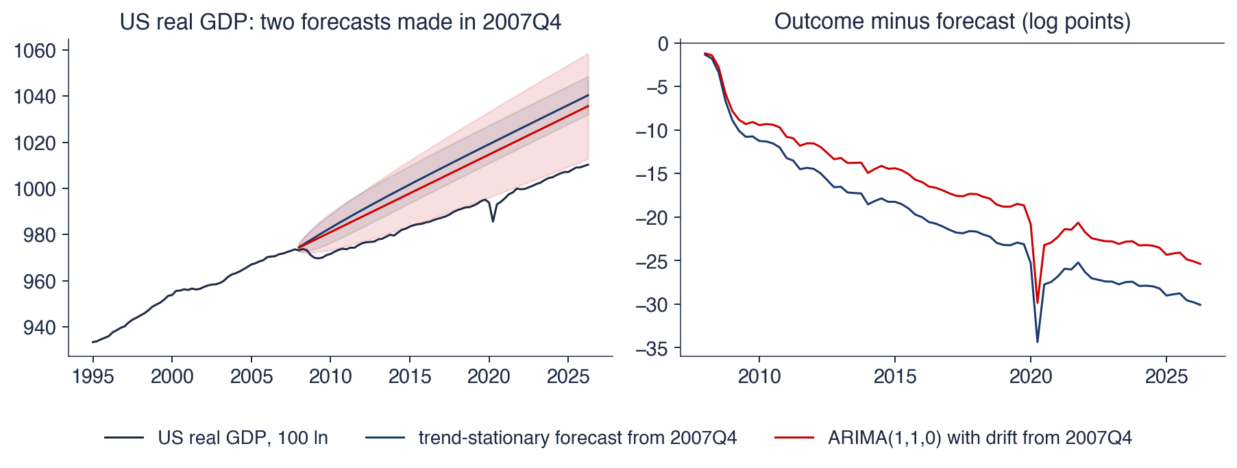
 TSA_ch3_trends